
The Effect of Spatially Correlated Errors on Sea Surface Height Retrieval from SWOT Altimetry
by

Max Yaremchuk
1,*,
Christopher Beattie
2,
Gleb Panteleev
1,
Joseph M. D’Addezio
1 and
Scott Smith
1 1
US Naval Research Laboratory, Stennis Space Center, MS 39522, USA
2
Department of Mathematics, Virginia Tech, Blacksburg, VA 24061, USA
*
Author to whom correspondence should be addressed.
Remote Sens. 2023, 15(17), 4277; https://doi.org/10.3390/rs15174277
Submission received: 12 July 2023
/
Revised: 24 August 2023
/
Accepted: 28 August 2023
/
Published: 31 August 2023
(This article belongs to the Special Issue Applications of Satellite Altimetry in Ocean Observation)
Abstract
:The upcoming technology of wide-swath altimetry from space will enable monitoring the ocean surface at 4–5 times better spatial resolution and 2–3 times better accuracy than traditional nadir altimeters. This development will provide a chance to directly observe submesoscale sea surface height (SSH) variations that have a typical magnitude of a few centimeters. Taking full advantage of this opportunity requires correct treatment of the correlated SSH errors caused by uncertainties in environmental conditions beneath the satellite and in the geometry and orientation of the on-board interferometer. These observation errors are highly correlated both along and across the surface swath scanned by the satellite, and this presents a significant challenge for accurate processing. In particular, the SWOT precision matrix has off-diagonal elements that are too numerous to allow standard approaches to remain tractable. In this study, we explore the utility of a block-diagonal approximation to the SWOT precision matrix in order to reconstruct SSH variability in the region east of Greenland. An extensive set of 2dVar assimilation experiments demonstrates that the sparse approximation proposed for the precision matrix provides accurate SSH retrievals when the background-to-observation error ratio ν does not exceed 3 and significant wave height is below 2.5 m. We also quantify the range of ν and significant wave heights over which the retrieval accuracy of the exact spatially correlated SWOT error model will outperform the uncorrelated model. In particular, the estimated range is found to be substantially wider ( with significant wave heights below 8–10 m), indicating the potential benefits of further improving the accuracy of approximations for the SWOT precision matrix.
1. Introduction
The Surface Water and Ocean Topography (SWOT, [1,2]) and Coastal and Ocean Measurement with Precise and Innovative Radar Altimeter (COMPIRA, [3]) missions are designed to deliver high resolution maps of ocean surface topography using radar interferometry. The SWOT satellite was launched on 16 December 2022, initially into a fast (1-day repeat cycle) sampling orbit for calibration, with plans for a later transition to an operational orbit having a longer (20.86-day) repeat cycle. The new type of observations of sea surface height (SSH) available from this satellite will deliver gridded data along 100–160 km-wide swaths at kilometer resolution.
In contrast to traditional nadir-based altimeters that were in operation in recent decades giving observed SSH anomalies with a typical error of 5–8 cm, this new remote sensing technology will have several times better SSH uncertainty of 2–3 cm. Achieving this precision requires taking into account additional spatially correlated observation errors of both instrumental and environmental origin. Processing data with spatial error correlations presents a certain challenge for operational data assimilation systems, mostly because of the huge dimension of the respective error covariance matrices. As an example, a transatlantic swath segment contains in the order of spatially correlated observations whose error covariance matrix will have (potentially) nonzero elements, creating a formidable demand on computational resources as a result.
In preparation for the SWOT mission, the Jet Propulsion Laboratory (JPL) developed an observation error covariance model [2,4] which has served as the basis for numerous experiments aimed at assessing the added value of the mission in monitoring global ocean dynamics (e.g., [5,6,7,8,9,10]). In these studies, simulated SWOT observations were assimilated into numerical models under the traditional assumption of a diagonal (i.e., spatially uncorrelated) error covariance matrix commonly adopted by operational data assimilation systems. However, in order to successfully resolve submesoscale SSH variations having typical magnitudes of a few centimeters, it is necessary to correctly take into account correlated errors, whose typical magnitudes are in the order of 1–2 cm. These errors are associated with uncertainties in the geometry and orientation of the interferometer, as well as with environmental factors, such as water vapor content in the atmospheric column between the satellite and the ocean surface.
In recent years, various approaches to denoising the SWOT signal from spatially correlated errors were considered (e.g., [11,12,13,14,15,16,17]). In particular, Ref. [11] explored various forms of high-order differential operators to penalize grid-scale components along the swath, while [12,13] proposed to filter SSH errors caused by the uncertainties in interferometer geometry and orientation by explicitly removing the corresponding across-swath modes from the observed SSH patterns. In a different approach, Ruggiero et al. [14] and Yaremchuk et al. [15] developed heuristic sparse approximations of the inverse error covariance matrix. More recently, separable [16] approximation to the SWOT error covariance matrix and block-diagonal (hereinafter BD) [17] approximation to its inverse square root have been developed.
In the present study, we explore the effect of taking spatially correlated SWOT errors into account in the presence of both mesoscale and submesoscale variability of the background field. The latter was simulated by a primitive equation model at 1 km resolution under various assumptions of the magnitude of the background error covariance. Based on a series of observation system simulation experiments (OSSEs), we evaluate the dependence of the assimilation skill on the magnitude of the mesoscale component in the background field, significant wave height, and observation-to-background error ratio.
The paper is organized as follows. In the next section we describe the structure of the SWOT error covariance matrix R developed by the Jet Propulsion Laboratory, as well as the sparse approximation of its inverse square root and the methodology of its numerical testing via 2dVar OSSEs. In Section 3 we compare the results of 2dVar retrievals of the reference fields with regard to different approximations of the inverse square root of R, including simple diagonal approximation, block-diagonal approximation, and exact inversion of the JPL covariance model. The findings are summarized and discussed in Section 4.
2. Setting of the Numerical Experiments
2.1. SWOT Error Covariance Model
The JPL error covariance model [6] is represented by the sum of three major constituents, associated with the errors caused by uncertainties in the geometry and orientation (GO) of the on-board interferometer, uncertainties in environmental conditions (state of the atmosphere and ocean waves), and the intrinsic noise of the Ka-band Radar Interferometer (KaRIn):
Here, , , and and denote the respective KaRIn, GO, and atmospheric error covariance matrices. In Equation (1), K is diagonal and has full rank whereas the other two components are positive semi-definite and may represent significant error correlations in both across- and along-swath directions. In the following, the across-swath and along-swath directions will be denoted, respectively, by x and y, and matrices associated with these directions will be labeled accordingly. In contrast to previous works on the approximation of (e.g., [16,17]), in this study we include atmospheric errors in cases where the uncertainty in the water vapor content is partly removed by twin radiometers ([4]). In accord with the JPL model, it is assumed that
Here, are the rank-one covariance matrices associated with across-swath uncertainties (namely, roll, phase, dilation, and timing), F is the Fourier transform in the directions of subscripts, , are the diagonal matrices with the respective error power spectra at the diagonals, and D is the operator removing the across-swath linear trend in the error field caused by the uncertainty of the water content in the atmosphere. The isotropic 2d spectrum in Equation (2) is the default spectrum from the SWOT simulator.
In [16,17] it has been shown that and its symmetric square root could be well-approximated by sparse block-diagonal matrices if the target SSH features have spatial scales below 30 km (i.e., spatial frequencies above 0.01 km). These features are well resolved by the SWOT interferometer, whose observation errors do not exceed 2–3 cm at 2 × 2 km grid resolutions. Availability of a numerically efficient approximation of provides an opportunity to inexpensively compute the normalized SWOT innovations in data assimilation systems, based on the inversion of correlations in data space (see Appendix A):
Here, δx is the SSH increment on the model grid, is the observation operator projecting the background state of the model on observations d, is its linearization in the vicinity of , is the diagonal matrix of the background error standard deviations, C is the background correlation matrix, and I is the identity matrix. Formulation (3) is routinely used in multi-variate data assimilation systems (e.g., [18]), as a (first-level) preconditioning. The transition of such systems to processing observations with non-diagonal error covariances requires either a substantial increase in computational power, or efficient approximations of . In this study, we employ an extensive set of OSSEs with the model SSH fields to explore the utility of the sparse approximation proposed in [17] by comparing its true state retrieval skill vs. the ones obtained using a diagonal approximation of and using its exact form. Since SSH has never been observed with zero error, the true ocean state was simulated by the output of a high-resolution primitive equation ocean model.
2.2. Ocean Simulations
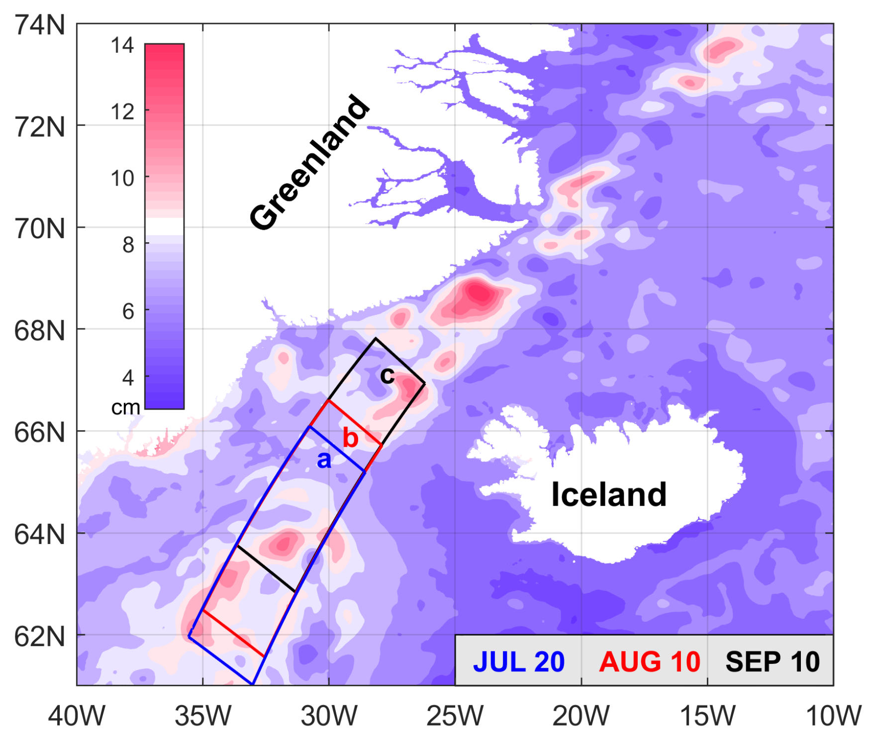
As mentioned above, the key added value of the SWOT altimeter is its higher spatial resolution and accuracy, which will enable oceanographers to directly observe submesoscale SSH variability in the open ocean and coastal environments. For this reason, we elected a high-latitude region (Figure 1) for testing the impact of the spatially correlated components of the SWOT error covariance matrix on the quality of SSH retrievals. The two major reasons for such a selection are the small (∼5–10 km) Rossby deformation radius and much smaller SSH variations (∼5–10 cm) at high latitudes relative, say, to larger values for each found in the tropics. These features present a challenge for monitoring SSH variability at high latitudes by nadir radiometers, whose spatial resolution and accuracy are barely consistent with eddy characteristics. At the same time, the retrieval quality of these features from SWOT data could be affected by correlated observation errors, whose magnitudes are comparable to those of the eddies, and, therefore, should be taken into account.
To simulate the “true” ocean, we used a 4-month output of the Navy Coastal Ocean Model (NCOM, [19]) in the Eastern Greenland Sea (Figure 1). The model was run at 1 km resolution between 1 June and 30 September 2019, nested within a coarser (4 km) configuration that was used to study the impact of freshwater runoff from the Greenland ice sheet on the local coastal circulation [20]. Apart from the runoff, the solution was forced by atmospheric fluxes of heat, freshwater, and momentum from the Navy Global Environmental Model (NAVGEM) [21]. To explore the impact of correlated SWOT errors on the retrieval quality of ocean states of various configuration, we picked three snapshots (Figure 2). The snapshots were extracted from the model hindcast on 20 July, 10 August, and 10 September 2019 at the three swath segments shown in Figure 1.
2.3. Methodology of the OSSEs
The numerical experiments were performed in a standard setting: First, the target “true” SSH fields were picked from the model and interpolated on 512 km-long segments (Figure 1) at 2 km resolution. Each field was 128 km-wide, contained 64 × 256 grid points, and enveloped a 120 km-wide swath segment of the SWOT satellite giving a total number of 12,800 observation locations, shown as a grid in the bottom panel of Figure 2. In this setting, simulated SWOT observations were collocated with the grid points of the background state. Second, the true fields at the SWOT observation locations were contaminated by an ensemble of 100 noise realizations generated by the SWOT simulator. The resulting “observed” fields were then used to retrieve true fields by computing corrections δx to the background SSH fields via Equation (3). For each member of the observation ensemble, a background field (simulating an uncertain “model forecast”) was specified by imposing background noise on the true solution, :
where n is a realization of the 2d Gaussian random field with zero mean and unit variance. is a diagonal matrix of (spatially homogeneous) standard deviations from the true fields, caused by simulated forecast errors. Similar to the SWOT errors, the model errors were assumed to be Gaussian with the correlation matrix
where Δ is the 2d Laplacian operator on the swath segment with Neumann boundary conditions, is the diagonal matrix of normalization factors (e.g., [22]) setting the diagonal of to 1, and a is the decorrelation scale.
The values of background noise, v, and decorrelation scale, a, were varied in the course of the experiments. Since the magnitude of SWOT errors depends on the significant surface wave height [6] (hereinafter SWH and denoted by w), and since SWH modulates the diagonal elements of K in Equation (2), the impact of surface waves on the accuracy of SSH retrievals was also assessed in an additional set of numerical experiments.
For each true field and each set of the retrieval parameters v, a, w, three ensembles of 2dVar assimilation experiments, which used three models of the square root of the SWOT precision matrix, were performed: (a) the exact JPL model based on Equation (2); (b) a block-diagonal model [17], allowing only for across-swath correlated errors; and (c) a diagonal approximation , which does not take any spatially correlated errors into account. The computation of a block-diagonal approximation was performed using a column-wise splitting scheme to compute an approximate precision matrix (see Appendix B) and then taking the square-roots of its diagonal blocks. This approach takes advantage of the specific structure of and allows for efficient parallelization in the along-swath direction.
The 2dvar retrieval skills of the true states were quantified using the error reduction ratios
Here, is the background error, angular brackets denote ensemble averages, an overline denotes the standard deviation of a field, and indices 0, 1, 2, 3 enumerate increments obtained using the exact (1), block-diagonal (2), and diagonal (3) models of , respectively. For the error reduction ratio, with respect to the background state, the index j is set to zero, implying that the increment (i.e., the skill) is assessed with respect to the background error, without assimilation.
3. Results
3.1. Sensitivity to Background Errors
The analysis Equation (3) can be rewritten in the equivalent form
providing better insight on the impact of the background errors on the results of assimilation. In particular, one may expect that, when the magnitude of (as measured by the sum of its eigenvalues, ) is much smaller than the uncertainties in the approximation of and, respectively, of in Equation (3), as measured, say, by ), will have a relatively small impact on the results of assimilation. For that reason, the ratio is likely to be a key parameter, controlling the accuracy of the SSH retrievals with various approximations of the precision matrix.
In our assimilation experiments, the background error magnitude v was measured in terms of the true states magnitude , while the background noise level was varied across the range between 0.2 and 0.8. The related norm of the background error covariance projection on SWOT observation points, , experienced variations between 1.3 and 21 m.
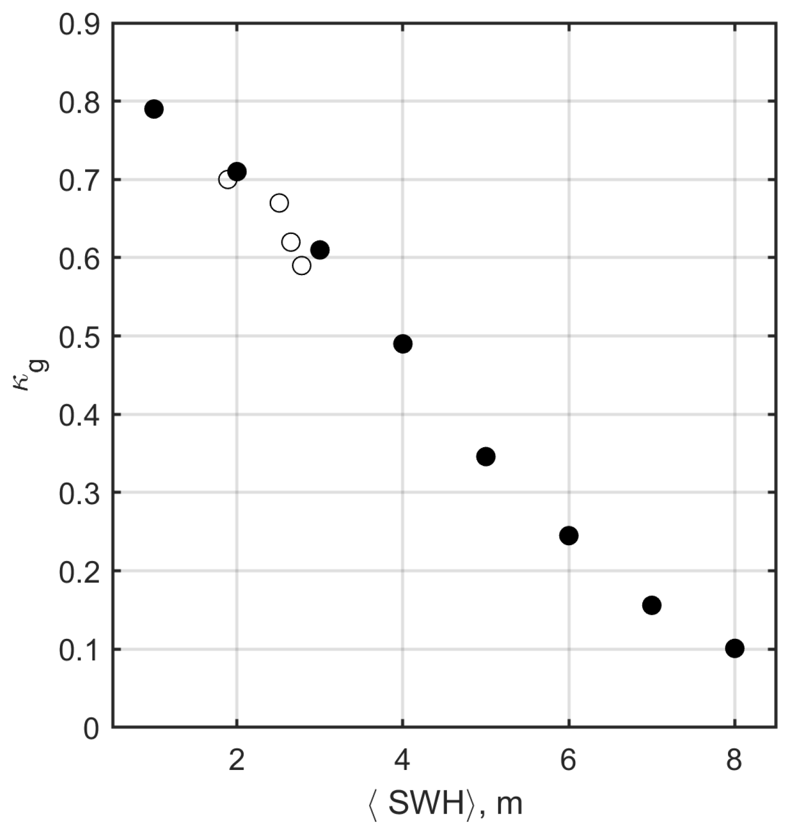
At the same time, varying the SWH magnitude, w, changed the observation noise level, , in an interval between 3 and 14 m. This range covered SWH changes ranging between calm seas (SWH = 1 m) to severe storm conditions (SWH = 8 m). It should be noted that, since the magnitude of the correlated errors in Equation (1) does not depend on SWH, their relative contribution to the SWOT covariance decreases with an increase in sea surface roughness (Figure 3), indicating a reduction in the diagonal approximation error due to growth of the diagonal dominance of R.
Figure 3 shows the potential importance of the proper treatment of spatially correlated errors in realistic conditions: SWH climatologies (e.g., [23,24]) indicate that there is more than a 95% chance of observing SWH below 4 m over the global ocean, with an average SWH value of about 1.8–2 m. These numbers correspond to 50–70% contribution of the correlated errors to the SWOT observation covariance. For calm sea conditions ( m), the contribution of KaRIn noise falls below 20% and becomes nearly negligible.
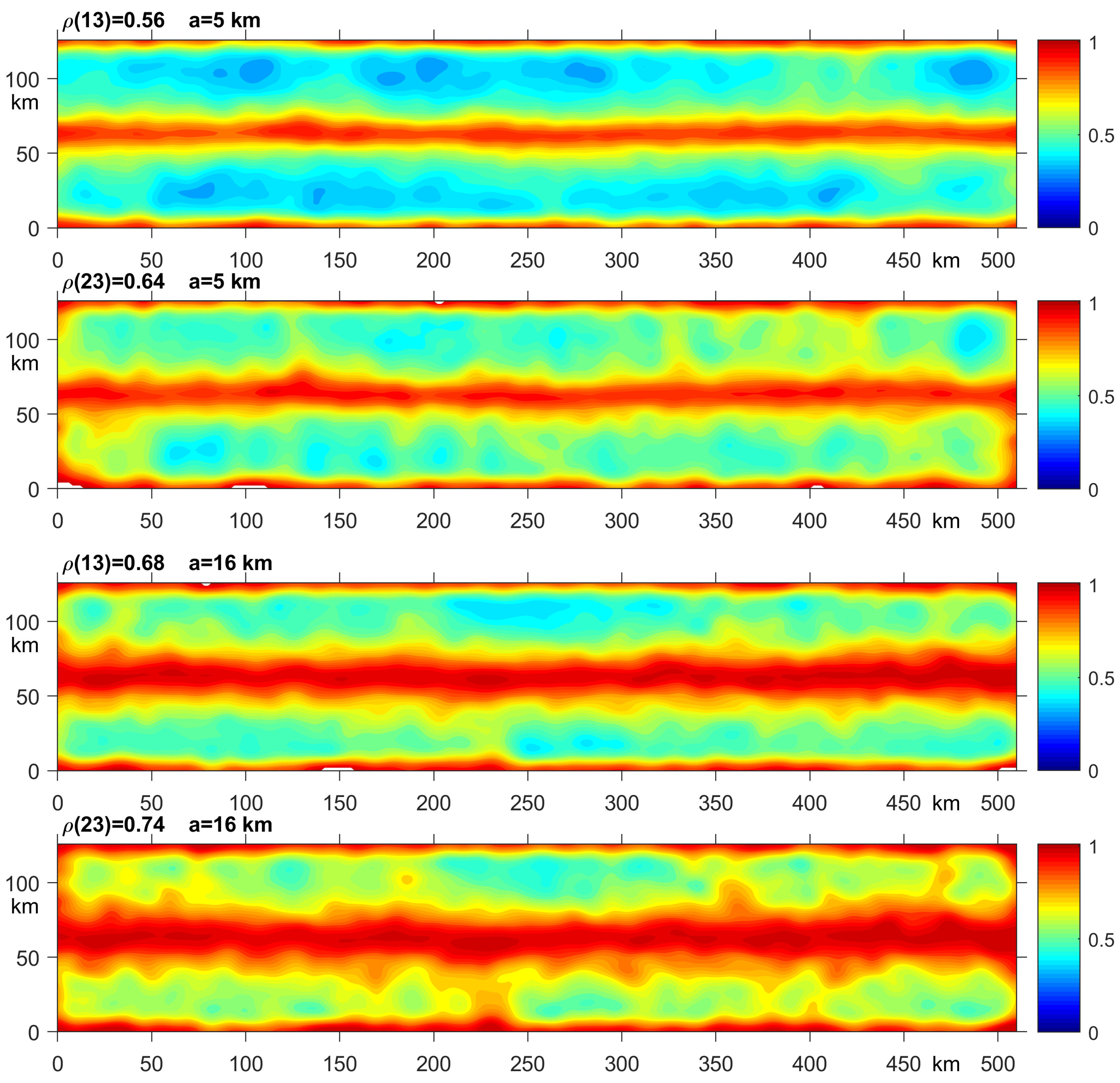
In the main series of experiments, we explored the dependence of the error reduction ratios (Equation (6)) on the decorrelation scale a of the background states. In the reference ensemble of 2dVar runs with the variable background noise level v, the value of a was set to the Rossby deformation radius, which is approximately 5 km for the summer stratification of the East Greenland Sea [25], and the SWH was set to a default constant value of 2 m. An example of typical error reductions , with respect to the errors obtained under the assumption of uncorrelated SWOT noise (diagonal approximation of the precision matrix), are shown in Figure 4 for the true state in Figure 2b. Similar distributions were obtained for the states displayed in Figure 2a,c.
As can be seen, both exact and approximate versions of the SWOT precision matrix demonstrate significantly better retrievals of the true SSH field with an ensemble-mean error reduction ratio persistently below 1 throughout the domain. Quantitatively, the area-mean ratio deteriorates from 0.55 to 0.72 with a 3-fold increase (from 5 to 16 km) of the background decorrelation scale, but nevertheless maintains persistent improvement of the analysis (values below 1) throughout the domain. Degradation of ρ caused by an increase in a primarily occurs due to error diffusion from the 10 km-wide nadir swath (that is unobserved by the interferometer) and the larger contribution of long-wave background error components to the overall error budget.
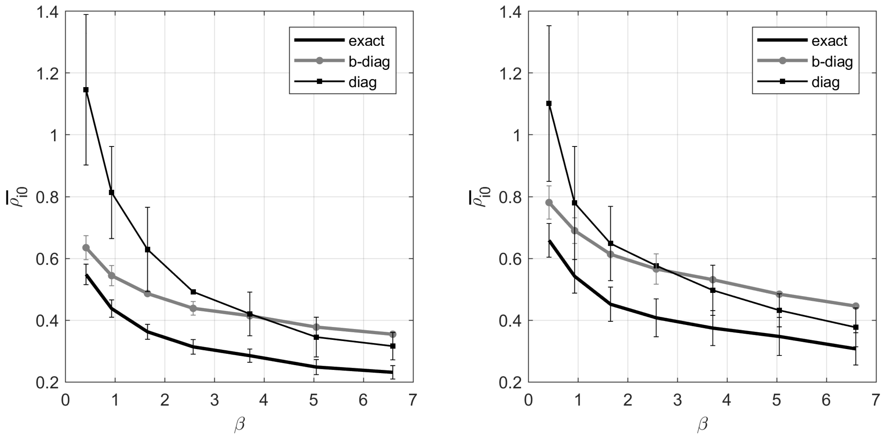
With an increase in ν, the patterns exposed in Figure 4 deteriorate, resulting in the gradual increase in up to 0.9 at . The value of characterizing the fidelity of the BD approximation eventually exceeds 1 (i.e., the BD approximation becomes indistinguishable from the diagonal representation of R) when the background-to-observation noise ratio β goes beyond a certain threshold, , whose magnitude depends on the values of a and SWH.
Figure 5 gives insight into the dependence of on the background decorrelation scale a for the most common case of 2 m waves. Irrespective of a, taking correlated errors into account appears to be prudent when the magnitude of observation errors exceeds those of the background (); in these cases, the diagonal approximation of R fails to substantially reduce the initial difference with the true state, keeping the reduction ratio (thin lines) within the range of 0.8–1.1. Increasing a from 5 to 16 km shrinks the range of applicability of the block-diagonal approximation from to . Although the exact form of (thick black lines in Figure 5) consistently demonstrates better skill than the diagonal approximation (thin lines), it eventually becomes worthless as the skill difference (thick-to-thin lines ratio) becomes statistically indistinguishable from 1 at fairly large values of ( > 12 for a = 5 km and for km). We assume that these effects are caused by the gradual saturation of the initial error field by the long-wave harmonics which tend to suppress visibility of the SWOT signal, whose errors are significantly correlated mostly on smaller scales. Nevertheless, it is obvious that using the exact SWOT error covariance is useful throughout the entire range of the background-to-observation noise ratio.
In practice, employing the exact SWOT covariance model in the analyses (Equations (3) and (7)) would be difficult because, typically, neither R nor are compactly representable in a way that is advantageous for inversion or solving linear systems. In particular, neither matrix will normally be sparse. The difficulties in dealing with this challenge could be relaxed to some extent by either using a BD approximation to , or in the case of rough seas, by recognizing the potential diagonal dominance of R due to the amplification of KaRIn noise (Figure 3) by surface waves.
3.2. Impact of Surface Waves
At first glance, increasing the diagonal dominance of R would improve the quality of the block-diagonal approximation of . However, this would be correct only in the case of relatively small background errors. In real situations, the latter often dominate the error balance in the analysis of Equations (3) and (7), so that inflating the diagonal of R would instead cause a rapid loss of information on the true state arriving from SWOT observations. This will, in turn, result in very small analysis increments (cf. Equation (3)).
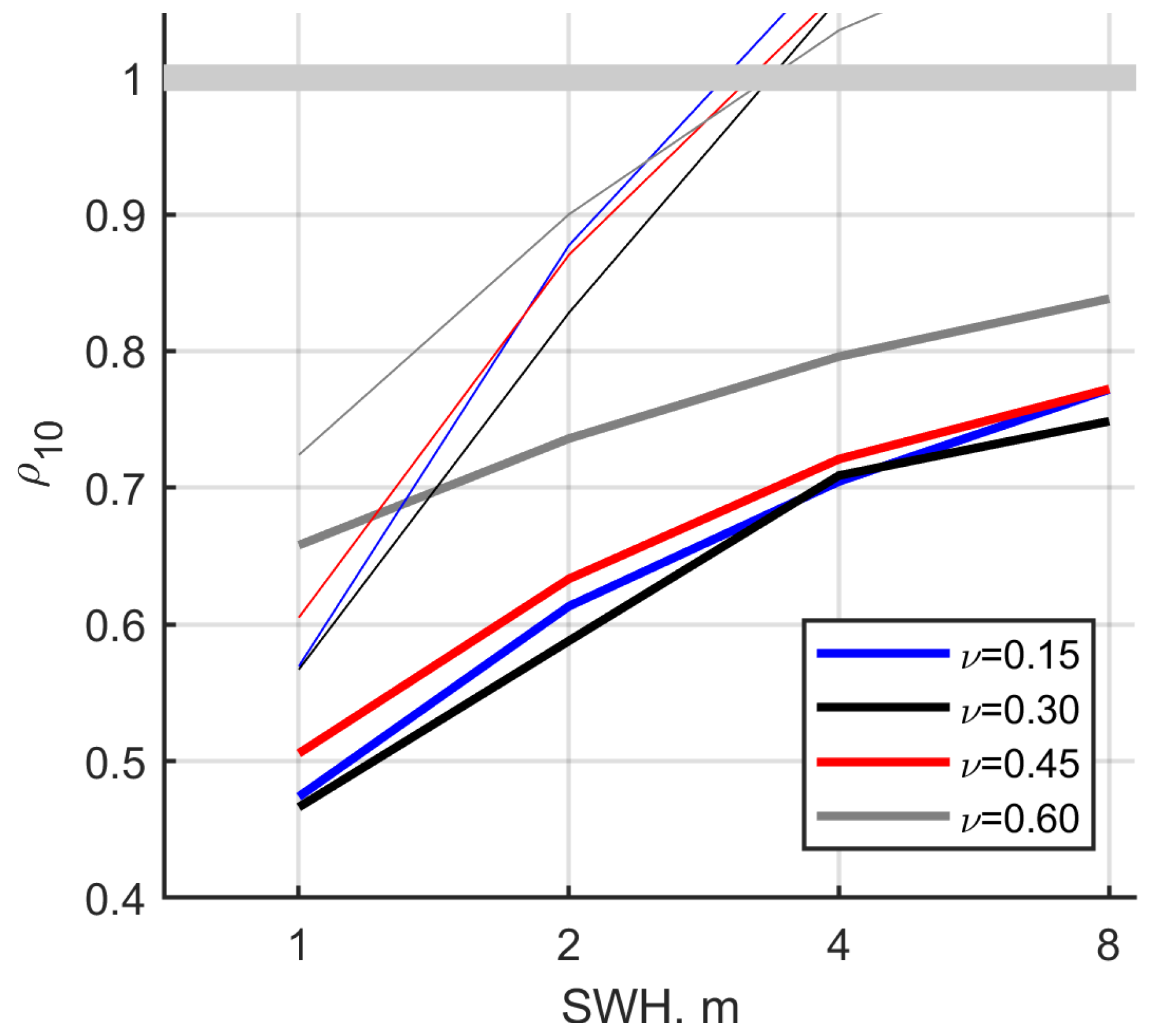
To study the impact of surface waves, we conducted a series of OSSEs using four spatially homogeneous SWH fields with w = 1, 2 4, and 8 m. In these experiments, the background noise level ν was varied in the range between 0.15 and 0.6, and the value of the background decorrelation scale a was 5, 8, and 16 km. The results of these OSSEs are displayed in Figure 6 for a = 5 and 8 km. It is remarkable that using the exact formulation of yields a quite significant (20–30%) amount of information on the true state, even for SWH = 8 m. For a calm sea (SWH = 1 m) and background noise levels of 0.15–0.3, SWOT observations provide on average more than two times better () approximation to the true states relative to background forecasts.
It is also notable that, under calm sea conditions ( m), the BD approximation of yields only a slightly (10–15%) worse retrieval skill compared to the exact case. However, with SWH growth, the BD skill deteriorates much faster, becoming nearly worthless for significant wave heights exceeding 2.5–3 m (thin lines in Figure 6). Despite this, the block-diagonal approximation appears to be applicable to SWOT data analysis over the entire globe with the exception of the Southern Ocean and high latitudes in the winter of the Northern Hemisphere [24].
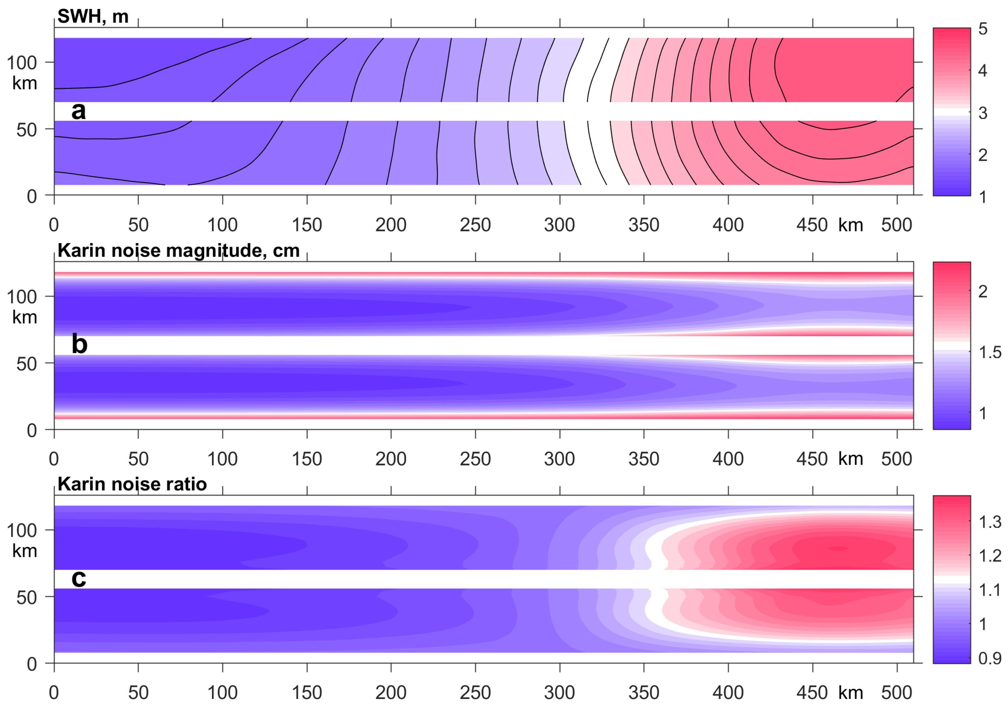
Results shown in Figure 6 were obtained with idealized (spatially homogeneous) SWH patterns over the swath. To assess the impact of SWH inhomogeneity, we conducted additional experiments by picking a realistic SWH distribution (Figure 7, upper panel) caused by a storm on 31 August 2019 (Copernicus Global Ocean Wave Reanalysis https://data.marine.copernicus.eu/product/GLOBAL_MULTIYEAR_WAV_001_032/description, (accessed on 11 July 2023)). Estimates of the respective true state retrieval skills were conducted for all of the states in Figure 2 and then compared with similar results obtained for the spatially averaged SWH of the pattern displayed in the upper panel of Figure 7.
The OSSEs demonstrated statistically insignificant differences in skill, and remained basically within the standard deviations around means produced by the respective 2dVar ensembles (see Table 1).
This result is due to two factors. First, the relative SWH variations across the swath are small because the typical horizontal scale of wind stress variation in the ocean is an order of magnitude larger than the swath half-width. Second, the response of the KaRIn noise magnitude to SWH variation is rather weak; in the test case considered, changes at most by a factor of two (middle panel in Figure 7b), whereas SWH varies by up to a factor of five over the same area. When combined, these factors produce relatively small (10–15%) variations in the KaRIn noise relative to the noise generated by the area-mean SWH (bottom panel in Figure 7). These small variations are further dispersed across the final skill estimates (Table 1) due to the presence of background errors in the analysis equation that are usually several times larger than observational ones.
4. Summary and Discussion
In this study, we investigated the retrieval skill of the BD approximation to the SWOT precision matrix using summer-time SSH variations in the East Greenland Sea. In contrast to the previous study [17], which focused on the retrieval of an idealized SSH variability at submesoscale, the tested background fields were characterized by wider spectra containing both mesoscale and submesoscale SSH variations in a realistic proportion. The retrieval skill of the BD approximation was assessed through the ensembles of 2dVar assimilation experiments with variable parameters of the error statistics in both SWOT observations and the background states.
The results of the study are summarized as follows. The correlated SWOT errors provide a significant contribution to the analysis if the background-to-observation noise ratio does not exceed 2.5–3 when the significant wave height is below 3 m. Above these levels, either SWOT observation information tends to be lost against the background noise and/or correlated errors become too small compared to the uncorrelated KaRIn noise, and, therefore, provide a negligible contribution to the structure of SSH signal to the analysis. The BD approximation to the SWOT precision matrix is especially efficient for calm seas (w < 1.5 m); with SWH growth, its validity quickly degrades and becomes virtually indistinguishable from the uncorrelated approximation of the SWH above 2–2.5 m. In contrast, employing the exact in the analysis persistently yields 20–60% better assimilation accuracy, even at rough seas (Figure 6). Finally, inhomogeneities of the SWH distribution along the swath weakly affect the analysis quality delivered by both the exact and BD approximations of the precision matrix.
The general, the conclusion is that SWOT-correlated errors, whose overall magnitude ranges within 1–3 cm, are most efficiently taken into account when the background SSH errors are below 5–7 cm and the SWH does not exceed 6–8 m. Otherwise, the diagonal approximation of the SWOT error covariance matrix will suffice in producing an essentially correct analysis.
Our experiments show that the computational cost of the BD approximation is significantly (30–50 times) less than when using the exact inversion of the SWOT error covariance. At the same time, the overall computational advantage of the diagonal approximation over the BD deteriorates, due to the necessity to compute the action of the (non-sparse) matrix B during the optimization process. As a result, the BD solutions are only 1.5–3 times more computationally expensive, depending on the decorrelation scale of the background error covariance. We also note that the computational efficiency of the BD approximation can be potentially improved by computing, in parallel, the action of the diagonal blocks on the observation vector along the satellite swath.
In the present study, we took into account correlated errors caused by the state of the atmosphere under the assumption that uncertainty in the atmospheric water content is partly removed by twin radiometers [6]. In this case, the residual atmospheric error is approximately two times smaller than . Therefore, its effect on the validity of the BD approximation would be minor. In that respect, it is worthwhile to note that adding the dry atmosphere errors (not yet implemented in the JPL model) is likely to expand the above limitations on the applicability of correlated errors in SSH retrieval.
Another important issue is the significant spectral gap between the mesoscale and submesoscale SSH variability in the open ocean. Usually, the SSH signature of mesoscale features is significantly larger than that of submesoscale features, resulting in a SWOT signal-to-background-noise ratio of , and, therefore, making it difficult to retrieve submesoscale features from a the mesoscale background. This will be true especially in the tropics, where the Rossby radius is much larger than in high latitudes. This difficulty could be relaxed to some extent in coastal regions by means of multi-scale data assimilation (e.g., [26,27]). In the latter approach, the mesoscale component of the increment δx is computed first, in order to update the background state under the diagonal approximation of the observation error covariances. After that, the (submesoscale) model-data misfits are reduced in magnitude and analyzed using a more sophisticated observation error model.
As an alternative to the linear framework used in the present study, SWOT errors could be filtered on the basis of neural networks [28,29] and other machine learning methods. This approach, however, requires the development of an extensive database spanning all configurations of the SSH fields on the satellite swaths, which is a considerable endeavor on its own. In addition, there is still a problem of independent in situ observations needed for calibration of all of the above-mentioned algorithms. Despite numerous experiments (e.g., [9,30]) conducted prior to the SWOT mission, more observational and numerical studies are still required for correct and accurate assessment of the SWOT error covariances.
Finally, our experiments indicate that utilization of the exact JPL model of R keeps performing better than the diagonal approximation up to the background noise levels of < 8–12 and significant wave heights less than 10 m. Therefore, it is quite important to further develop numerically efficient approximations to by exploiting symmetries in the structure of R, which is the subject of our current studies.
Author Contributions
Conceptualization, M.Y.; Methodology, M.Y. and C.B.; Software, M.Y., C.B., G.P. and J.M.D.; Formal analysis, G.P. and J.M.D.; Data curation, S.S.; Writing—original draft, M.Y. All authors have read and agreed to the published version of the manuscript.
Funding
This research was funded by the ONR project number 73-6C95025 “Precision assessment of Remotely Sensed data with Error Correlations” (PARSEC). CB was supported by NSF Grant DMS-1923221 and the ONR Summer Faculty Fellowship Program.
Data Availability Statement
The model data presented in this study are securely stored at the Navy DSRC archive serevr and can be accessed after obtaining of the account at the facility. Scott Smith can be contacted for information to access the archived data once an account has been extablished.
Conflicts of Interest
The authors declare no conflict of interest.
Appendix A. H-Preconditioned Formulation of the Optimization Problem
The observation space solution δx to the least squares problem
is given by Equation (7). The condition number of the system matrix can be improved by representing the background error covariance in the form (Equation (7)). and transforming the observation operator
in accordance with the right relationship in Equation (3). Substitution of (A2) into Equation (7) yields Equation (3):
Appendix B. Block-Diagonal Approximation of the SWOT Precision Matrix
Since the SWOT covariance matrix R is symmetric, we look for an approximation to in the form of a symmetric block-diagonal matrix with diagonal blocks each of size . We denote the set of such matrices by , and seek a solution to
Partition as , where each denotes the kth block column of having the dimension . Partition the identity in the same manner and write , where each is a symmetric matrix. In this case,
Evidently, each term within the sum can be minimized independently. Perform a singular value decomposition of each for . Here, is an matrix of orthonormal vectors, is a diagonal matrix of singular values, , and is an unitary matrix. The individual norms under the sum in (A5) can then be rewritten as
where we have made use of the unitary invariance of the Frobenius norm in (A6) and the Pythagorean Theorem in (A7). Introduce the substitutions, and . Noting that the second term in (A7) does not depend on , one may minimize , taking into account the symmetry of , simply by minimizing the first term, , subject to the equivalent constraint that be symmetric. This, in turn, can be accomplished via the method of Lagrange multipliers, producing ultimately an optimal symmetric having (i, j) elements given explicitly as
The optimal (symmetric) solution is then given by . Significantly, the solution to the originally posed problem (A4) can be solved in parallel by minimizing the independent subproblems, , as described above. This can be carried out in parallel with minimal data motion and synchronization. Notice further that an approximation to the inverse square root of is available by computing immediately the (symmetric) square roots of the individual blocks , for so that, .
References
- Durand, M.; Fu, L.L.; Lettenemaier, D.; Alsdorf, D.; Rodriguers, E.; Esteban-Fernandez, D. The surface water and ocean topography mission: Observing terrestrial surface water and oceanic submesoscale eddies. Proc. IEEE 2010, 98, 766–779. [Google Scholar] [CrossRef]
- Esteban-Fernandez, D. SWOT Project: Mission Performance and Error Budge; Revision A; NASA/JPL Tech. Rep. JPL D-79084. 2013; 83p. Available online: http://swot.jpl.nasa.gov/files/SWOT_D-79084_v5h6_SDT.pdf (accessed on 11 July 2023).
- Ito, N.; Uematsu, A.; Yajima, Y.; Isoguchi, O. A Japanese new altimetry mission COMPIRA—Towards high temporal and spatial sampling of sea surface height. In Proceedings of the AGU Fall Meeting, San Francisco, CA, USA, 15–19 December 2014. Abstract OS34B-05. [Google Scholar]
- Gaultier, L.; Ubelmann, C.; Fu, L.-L. SWOT Simulator Documentation; Tech. Rep. 2.3.0; Jet Propulsion Laboratory: Pasadena, CA, USA, 2017.
- Chelton, D.B.; Samelson, R.M.; Farrar, J.T. The effects of uncorrelated measurement noise on SWOT estimates of sea surface height, velocity, and vorticity. J. Atmos. Ocean. Technol. 2022, 38, 1053–1083. [Google Scholar] [CrossRef]
- Gaultier, L.; Ubelmann, C.; Fu, L.-L. The challenge of using future SWOT data for oceanic field reconstruction. J. Atmos. Ocean. Technol. 2016, 33, 119–126. [Google Scholar] [CrossRef]
- Li, Z.; Wang, J.; Fu, L.-L. An observing system simulation experiment for ocean state estimation to assess the performance of the SWOT mission: Part 1—A twin experiment. J. Geophys. Res. Oceans 2019, 124, 4838–4855. [Google Scholar] [CrossRef]
- Ubelmann, C.; Klein, E.; Fu, L. Dynamic interpolation of sea surface height and potential applications for future high-resolution altimetry mapping. J. Atmos. Ocean. Technol. 2015, 32, 177–184. [Google Scholar] [CrossRef]
- Wang, J.; Fu, L.L.; Qui, B.; Menemenlis, D.; Farrar, J.T.; Chao, Y.; Thompson, A.F.; Flexas, M.M. An observing system simulation experiment for the calibration and validation of the SWOT sea surface height measurement using in situ platforms. J. Atmos. Ocean. Technol. 2018, 35, 281–297. [Google Scholar] [CrossRef]
- Ma, C.; Guo, X.; Zhang, H.; Di, J.; Chen, G. An investigation of the influences of SWOT sampling and errors on ocean eddy observation. Remote Sens. 2020, 12, 2682. [Google Scholar] [CrossRef]
- Gomez-Navarro, L.; Cosme, E.; Somme, J.L.; Papadakis, N.; Pascual, A. Development of an image denoising method in preparation for SWOT satellite mission. Remote. Sens. 2020, 12, 734. [Google Scholar] [CrossRef]
- Metref, S.; Cosme, E.; Sommer, J.L.; Poel, N.; Brankart, J.-M.; Verron, J.; Navarro, L.G. Reduction of spatially structured errors in wide-swath altimetric satellite data using data assimilation. Remote Sens. 2019, 11, 1336. [Google Scholar] [CrossRef]
- Metref, S.; Cosme, E.; Guillou, F.L.; Sommer, J.L.; Brankart, J.-M.; Verron, J. Wide-swath altimetric satellite data assimilation with correlated error reduction. Front. Mar. Sci. 2020, 6, 822. [Google Scholar] [CrossRef]
- Ruggiero, G.A.; Cosme, E.; Brankart, J.M.; Le Sommer, J.; Ubelmann, C. An efficient way to account for observation error correlations in the assimilation of data from the future SWOT high-resolution altimeter mission. J. Atmos. Ocean. Technol. 2016, 33, 2755–2768. [Google Scholar] [CrossRef]
- Yaremchuk, M.; D’Addezio, J.; Panteleev, G.; Jacobs, G. On the approximation of the inverse error covariances of high-resolution altimetry data. Q. J. R. Meteorol. Soc. 2018, 144, 1995–2000. [Google Scholar] [CrossRef]
- Yaremchuk, M.; D’Addezio, J.; Jacobs, G. Facilitating inversion of the error covariance models for the wide-swath altimeters. Remote Sens. 2020, 12, 1823. [Google Scholar] [CrossRef]
- Yaremchuk, M. Sparse approximation of the precision matrices for the wide-swath altimeters. Remote Sens. 2022, 14, 2827. [Google Scholar] [CrossRef]
- Cummings, J.A.; Smedstad, O.M. Variational data analysis for the global ocean. In Data Assimilation for Atmospheric, Oceanic and Hydrologic Applications; Park, S.K., Xu, L., Eds.; Springer: Berlin/Heidelberg, Germany, 2013; Volume II. [Google Scholar] [CrossRef]
- Barron, C.N.; Kara, A.B.; Martin, P.J.; Rhodes, R.C.; Smedstad, L.F. Formulation, implementation and examination of vertical coordinate choices in the Global Navy Coastal Ocean Model (NCOM). Ocean. Model. 2006, 11, 347–375. [Google Scholar] [CrossRef]
- Helber, R.W.; Smith, S.R.; Panteleev, G.; Shriver, J.; Pickard, R. Greenland Freshwater Stability in the East Greenland Current. Deep-Sea Res. I 2023. under review. [Google Scholar]
- Hogan, T.F.; Liu, M.; Ridout, J.A.; Peng, M.S.; Whitcomb, T.R.; Ruston, B.C.; Reynolds, C.A.; Eckermann, S.D.; Moskaitis, J.R.; Baker, N.L.; et al. The Navy Global Environmental Model. Oceanography 2014, 27, 116–125. [Google Scholar] [CrossRef]
- Yaremchuk, M.; Carrier, M.; Smith, S.; Jacobs, G. Background error correlation modeling with diffusion operators. In Data Assimilation for Atmospheric, Oceanic and Hydrologic Applications; Park, S.K., Xu, L., Eds.; Springer: Berlin/Heidelberg, Germany, 2013; Volume II, pp. 177–203. [Google Scholar] [CrossRef]
- Colosi, L.V.; Bôas, A.B.V.; Gille, S.T. The Seasonal cycle of significant wave height in the ocean: Local versus remote forcing. J. Geophys. Res. 2021, 126, e2021JC017198. [Google Scholar] [CrossRef]
- Lemos, G.; Semedo, A.; Dobrynin, M.; Behrens, A.; Staneva, J.; Bidlot, J.-R.; Miranda, P.M.A. Mid-twenty-first century global wave climate projections: Results from a dynamic CMIP5 based ensemble. Glob. Palnetary Chang. 2019, 172, 69–87. [Google Scholar] [CrossRef]
- Nurser, A.J.G.; Bacon, S. The Rossby radius in the Arctic Ocean. Ocean Sci. 2014, 10, 967–975. [Google Scholar] [CrossRef]
- Li, Z.; McWiliams, J.C.; Ide, K.; Farrara, J.D. A multi-scale variational data assimilation scheme: Formulation and illustration. Mon. Wea. Rev. 2015, 143, 3804–3822. [Google Scholar] [CrossRef]
- de Moraes, R.J.; Hajibeygi, H.; Jansen, J.D. A multiscale method for data assimilation. Comput. Geosci. 2020, 24, 425–442. [Google Scholar] [CrossRef]
- Febvre, Q.; Ubelmann, C.; Sommer, J.L.; Fablet, R. Scale-aware neural calibration for wide swath altimetry observations. arXiv 2023, arXiv:2302.04497v2. [Google Scholar]
- Tréboutte, A.; Carli, E.; Ballarotta, M.; Carpentier, B.; Faugère, Y.; Dibarboure, G. KaRIn noise reduction using a convolutional neural network for the SWOT ocean products. Remote Sens. 2023, 15, 2183. [Google Scholar] [CrossRef]
- Wang, J.; Fu, L.-L.; Haines, B.; Lankhorst, M.; Lucas, A.J.; Farrar, J.T.; Send, U.; Meinig, C.; Schofield, O.; Ray, R.; et al. On the development of SWOT in-situ Calibration/Validation of the short-wavelength ocean topography. J. Atmos. Ocean. Technol. 2022, 39, 595–617. [Google Scholar] [CrossRef]
Figure 1.
Model domain and swath segments used in OSSEs. The field of temporal RMS variations of the SSH is shown by color shading on the background. Labels a, b, and c denote locations of model snapshots extracted from the hindcast on 20 July (a), 10 August (b), and 5 September (c), 2019.
Figure 1.
Model domain and swath segments used in OSSEs. The field of temporal RMS variations of the SSH is shown by color shading on the background. Labels a, b, and c denote locations of model snapshots extracted from the hindcast on 20 July (a), 10 August (b), and 5 September (c), 2019.

Figure 2.
The true SSH fields used in the assimilation experiments. The simulation dates and swath segment labels (Figure 1) are shown. Sampling of these fields by simulated SWOT observations is shown by dots in the bottom panel only. Units are in meters.
Figure 2.
The true SSH fields used in the assimilation experiments. The simulation dates and swath segment labels (Figure 1) are shown. Sampling of these fields by simulated SWOT observations is shown by dots in the bottom panel only. Units are in meters.

Figure 3.
Contribution κ of the correlated errors to the SWOT covariance for spatially homogeneous (black circles) and inhomogeneous (open circles) distributions of the SWH over the swath segment b shown in Figure 1.
Figure 3.
Contribution κ of the correlated errors to the SWOT covariance for spatially homogeneous (black circles) and inhomogeneous (open circles) distributions of the SWH over the swath segment b shown in Figure 1.

Figure 4.
Spatial distributions of relative error reduction ratios for the exact (1st and 3rd panels from the top) and block-diagonal (2nd and 4th panels) approximation of and . The horizontal decorrelation scale a of the background error covariance and the horizontally averaged values of are shown.

Figure 5.
Dependence of the error reduction ratios on the relative magnitude β of the background-to-observation error for km (left) and km (right). The error bars derived from the respective ensembles of 2dVar assimilations are shown.
Figure 5.
Dependence of the error reduction ratios on the relative magnitude β of the background-to-observation error for km (left) and km (right). The error bars derived from the respective ensembles of 2dVar assimilations are shown.

Figure 6.
Dependence of the true state retrieval error on SWH for the exact (, solid lines) and block-diagonal (, thin lines) approximations of for the gradually increasing noise levels ν of the background error. The OSSE results shown are averaged over the three true states in Figure 2.
Figure 6.
Dependence of the true state retrieval error on SWH for the exact (, solid lines) and block-diagonal (, thin lines) approximations of for the gradually increasing noise levels ν of the background error. The OSSE results shown are averaged over the three true states in Figure 2.

Figure 7.
From top to bottom: (a) SWH map w(x, y) during the storm observed on 31 August 2019; (b) the respective map of the diagonal elements of ; (c) the diagonal of where is KaRIn noise variance when SWH is spatially homogeneous and equal to the horizontal average (2.8 m) of the pattern shown in the upper panel.


Table 1.
Mean retrieval skills for various combinations of the background error decorrelation scale a and noise level ν. The asterisks in the column headers denote spatially homogeneous versions of K in the assimilation experiments with exact (E, bold), block-diagonal (B, italic), and diagonal (D) versions of . Table entries are the retrieval skills averaged over the ensembles of assimilations for the three true states shown in Figure 2.
| a, km | E | E | B | B | D | D | |
|---|---|---|---|---|---|---|---|
| 5 | 0.15 | 0.57 ± 0.02 | 0.58 ± 0.02 | 0.66 ± 0.02 | 0.67 ± 0.03 | 1.09 ± 0.22 | 1.11 ± 0.21 |
| 5 | 0.30 | 0.39 ± 0.02 | 0.39 ± 0.02 | 0.52 ± 0.02 | 0.53 ± 0.02 | 0.62 ± 0.11 | 0.63 ± 0.12 |
| 8 | 0.15 | 0.55 ± 0.04 | 0.56 ± 0.04 | 0.66 ± 0.04 | 0.67 ± 0.05 | 1.11 ± 0.25 | 1.13 ± 0.24 |
| 8 | 0.30 | 0.37 ± 0.03 | 0.37 ± 0.03 | 0.51 ± 0.03 | 0.51 ± 0.04 | 0.60 ± 0.12 | 0.61 ± 0.13 |
Disclaimer/Publisher’s Note: The statements, opinions and data contained in all publications are solely those of the individual author(s) and contributor(s) and not of MDPI and/or the editor(s). MDPI and/or the editor(s) disclaim responsibility for any injury to people or property resulting from any ideas, methods, instructions or products referred to in the content. |
© 2023 by the authors. Licensee MDPI, Basel, Switzerland. This article is an open access article distributed under the terms and conditions of the Creative Commons Attribution (CC BY) license (https://creativecommons.org/licenses/by/4.0/).
Share and Cite
MDPI and ACS Style
Yaremchuk, M.; Beattie, C.; Panteleev, G.; D’Addezio, J.M.; Smith, S. The Effect of Spatially Correlated Errors on Sea Surface Height Retrieval from SWOT Altimetry. Remote Sens. 2023, 15, 4277. https://doi.org/10.3390/rs15174277
AMA Style
Yaremchuk M, Beattie C, Panteleev G, D’Addezio JM, Smith S. The Effect of Spatially Correlated Errors on Sea Surface Height Retrieval from SWOT Altimetry. Remote Sensing. 2023; 15(17):4277. https://doi.org/10.3390/rs15174277
Chicago/Turabian StyleYaremchuk, Max, Christopher Beattie, Gleb Panteleev, Joseph M. D’Addezio, and Scott Smith. 2023. "The Effect of Spatially Correlated Errors on Sea Surface Height Retrieval from SWOT Altimetry" Remote Sensing 15, no. 17: 4277. https://doi.org/10.3390/rs15174277
Note that from the first issue of 2016, this journal uses article numbers instead of page numbers. See further details here.