Article

Enhancing Solar-Induced Fluorescence Interpretation: Quantifying Fractional Sunlit Vegetation Cover Using Linear Spectral Unmixing

by
Adrián Moncholi-Estornell
1,*,
Maria Pilar Cendrero-Mateo
1,
Michal Antala
2,
Sergio Cogliati
3,
José Moreno
1 and
Shari Van Wittenberghe
1
1
Laboratory of Earth Observation, Image Processing Laboratory, University of Valencia, C/Catedrático Agustin Escardino, n° 9, 46980 Paterna, Spain
2
Laboratory of Bioclimatology, Department of Ecology and Environmental Protection, Faculty of Environmental Engineering and Mechanical Engineering, Poznan University of Life Sciences, Piatkowska 94, 60-649 Poznan, Poland
3
Remote Sensing of Environmental Dynamics Lab., DISAT, University of Milano-Bicocca, Piazza della Scienza 1, 20126 Milan, Italy
*
Author to whom correspondence should be addressed.
Remote Sens. 2023, 15(17), 4274; https://doi.org/10.3390/rs15174274
Submission received: 25 July 2023 / Revised: 25 August 2023 / Accepted: 29 August 2023 / Published: 31 August 2023
(This article belongs to the Section Remote Sensing in Agriculture and Vegetation)

Abstract

:
Solar-induced chlorophyll fluorescence (SIF) is closely related to plant photosynthetic activity and has been used in different studies as a proxy for vegetation health status. However, in order to use SIF as a relevant indicator of plant physiological stress, it is necessary to accurately quantify the amount of light absorbed by the photosynthetic plant pigments, called the absorbed photosynthetically active radiation (APAR). The ratio between fluorescence emission and light absorption (i.e., SIF and APAR) is known as the fluorescence quantum efficiency (FQE). In this work, simultaneous measurements of SIF and reflected radiance were performed both at the leaf and canopy levels for Salvia farinacea and Datura stramonium plants. With the aim of disentangling the proportion of sunlit and shaded absorbed PAR, an ad hoc experimental setup was designed to provide a wide range of fraction vegetation cover (FVC) canopy settings. A linear spectral unmixing method was proposed to estimate the contribution of soil, sunlit, and shaded vegetation from the total reflectance spectrum measured at the canopy level. Later, the retrieved sunlit FVC (FVCsunlit) was used to estimate the (dominant) green APAR flux, and this was combined with the integral of the spectrally resolved fluorescence to calculate the FQE. The results of this study demonstrated that under no-stress conditions and independently of the FVC, similar FQE values were observed when SIF was properly normalised by the green APAR flux. The results obtained showed that the reflectance spectra retrieved using a linear unmixing method had a maximum RMSE of less than 0.03 along the spectrum. The FVCsunlit evaluation showed an RMSE of 14% with an R2 of 0.84. Moreover, the FQE values obtained at the top of the canopy (TOC) were found statistically comparable to the reference values at the leaf level. These results support further efforts to improve the interpretation of fluorescence based on field spectroscopy and the further upscaling to imaging spectroscopy at airborne and satellite levels.

1. Introduction

Under the current conditions of climate change, the early detection of crop and global vegetation stress is crucial to promote a sustainable agriculture and ecosystem management. With the upcoming European Space Agency’s Fluorescence Explorer (FLEX) and Sentinel 3 tandem mission [1], vegetation fluorescence and the auxiliary parameters needed to interpret solar-induced vegetation fluorescence (SIF) will be available at a 300 × 300 m spatial resolution. SIF is primarily controlled by the amount of light reaching the photosynthetic surface (absorbed by chlorophyll a (Chl a) molecules). At the photosystem level, given the same absorbed photosynthetically active radiation (APAR) and regardless of the species studied and the leaf structure, a relatively constant fluorescence emission is expected, driven by the change in fluorescence quenching [2,3]. At the leaf level, different studies have shown a similar fluorescence quantum efficiency (FQE) (i.e., the flux of fluorescence photons normalised by the flux of absorbed photons) when plants had a similar chlorophyll content and were grown under the same environmental conditions (i.e., light history and stress conditions) [4,5,6]. However, at the canopy level, the vegetation structure distorts both, the light reaching the photosynthetic surface (affecting the photosynthetic reactions) and the fluorescence signal (emitted by the vegetation) measured at the top of the canopy (TOC). Therefore, before using remote measurements of SIF to determine the plant physiological status, three major challenges need to be overcome: (i) quantifying the amount of light incident on the photosynthetic surface, (ii) quantifying the amount of light absorbed by Chl a molecules or the green/photosynthetically active surface, and (iii) correcting the measured top of the canopy fluorescence by canopy scattering and reabsorption [7,8,9,10,11]. This study will focus on the first and second challenges (research question I—RQ I), with the ultimate goal of a remote estimation of the FQE (research question II—RQ II), which is going beyond fluorescence for early stress detection.
Regarding RQ I, fluorescence and photosynthesis are coupled by the actual amount of light reaching the photosynthetic surface. Under normal growing conditions, the quantity and quality of photosynthetically active radiation (PAR) varies within the canopy profile. Moreover, shade-adapted leaves often have higher Chl contents and tend to be larger and thinner than sun-adapted leaves [12]. The biophysical and structural leaf heterogeneity results in a different light spectral response and leaf reflectance. Previous studies have shown that an inaccurate characterization of the at-target incoming radiance leads to an over- or underestimation of the retrieved vegetation properties when using reflectance indices due to a biased incoming radiance estimation [13]. While inaccuracies in the estimation of the at-target PAR do not alter the relationship between SIF and photosynthesis, an accurate quantification of the flux of photons reaching the photosynthetic surface is essential for a mechanistic interpretation of SIF [14].
Hence, at the canopy level, the main factors influencing the light received by the photosynthetic surface are the vegetation’s structural properties such as the fraction of vegetation cover (FVC), leaf area index (LAI), and leaf angle distribution function (LADF) [15]. A different vegetation structure leads to a different vertical distribution of light, resulting in different proportions of shaded and sunlit leaves observed within the canopy. The fluorescence flux measured from the top of the canopy integrates both the fluorescence emitted by the sunlit and shaded fractions of the canopy. Based on previous studies, we assume that when measuring from the nadir, sunlit leaves dominate the measured total fluorescence flux [16,17]. Therefore, we hypothesise that by accounting for the proportion of light reaching the sunlit and shaded leaves, as well as nonvegetated surfaces such as soil and woody material (RQ I), the remote estimation of the FQE estimates will be improved (RQ II).
To solve RQ I, the scientific community has developed several remote sensing methods to distinguish between the surface components described above [18,19,20]. For instance, the methods based on spectral mixture analysis (SMA) define the different components of a scene as endmembers with a relatively constant spectral signature. The process of quantifying the abundance of each endmember in the total measured spectrum is known as unmixing. Unmixing methods range from the use of linear spectral combinations [21] to machine learning approaches [22], including the use of spectral indices [23].
Linear unmixing consists of estimating the contribution of each endmember in a given spectrum based on a linear combination of them. Therefore, the measured TOC reflected radiance, if not strongly affected by multiple scattering due to complex vertical structure [18,24,25], can be defined as a linear combination of four surface components: the vegetation sunlit and shaded fraction as well as the soil sunlit and shaded fraction [26,27,28,29]. SMA has long been used to analyse hyperspectral images for ecological studies [25,30]. Based on this approach, methods such as residual spectral unmixing [31] have been developed to obtain soil properties from hyperspectral measurements. In addition, other authors have proposed the non-negative matrix factorization (NMF) to quantify soil salt content [32] or wheat biomass [33] as an example of other SMA techniques.
The spatial resolution of remote hyperspectral sensors implies mixed surface pixels (i.e., consisting of sunlit and shaded leaves, soil and woody material). External ancillary data could be used to determine the spatial heterogeneity of the canopy, but this involves differences in the values obtained due to different illumination and observation angles and temporal dynamics, especially relevant at the satellite level. To overcome these limitations, and in the context of the FLEX mission, we hypothesise that by taking advantage of the benchmark high-spectral resolution sensors and the linear spectral unmixing method, we will be able to quantify the sunlit canopy fraction (FVCsunlit), which is necessary to calculate the effective APAR flux at the canopy level [9,34] (RQ I) to obtain the FQE from remote sensing techniques (RQ II).
With the aim to evaluate the proposed hypothesis, an experiment is designed with a wide range of vegetation fractional cover scenarios, using well-watered potted plants of two different species, characterized by different leaf size and canopy density. Regarding RQ II, as previously introduced, since both species will be measured under the same environmental conditions, we hypothesise that a similar FQE will be obtained at the leaf and canopy scales, regardless of the different FVC. As described in previous studies [9,14,35], further processing and normalisation of initially derived stress proxies such as SIF can lead to a more detailed early stress detection directly related to photosynthetic light responses and a further global carbon assessment. These developments directly support the global monitoring of early vegetation stress using remote sensing techniques.

2. Materials and Methods

2.1. Plant Material and Experimental Setup

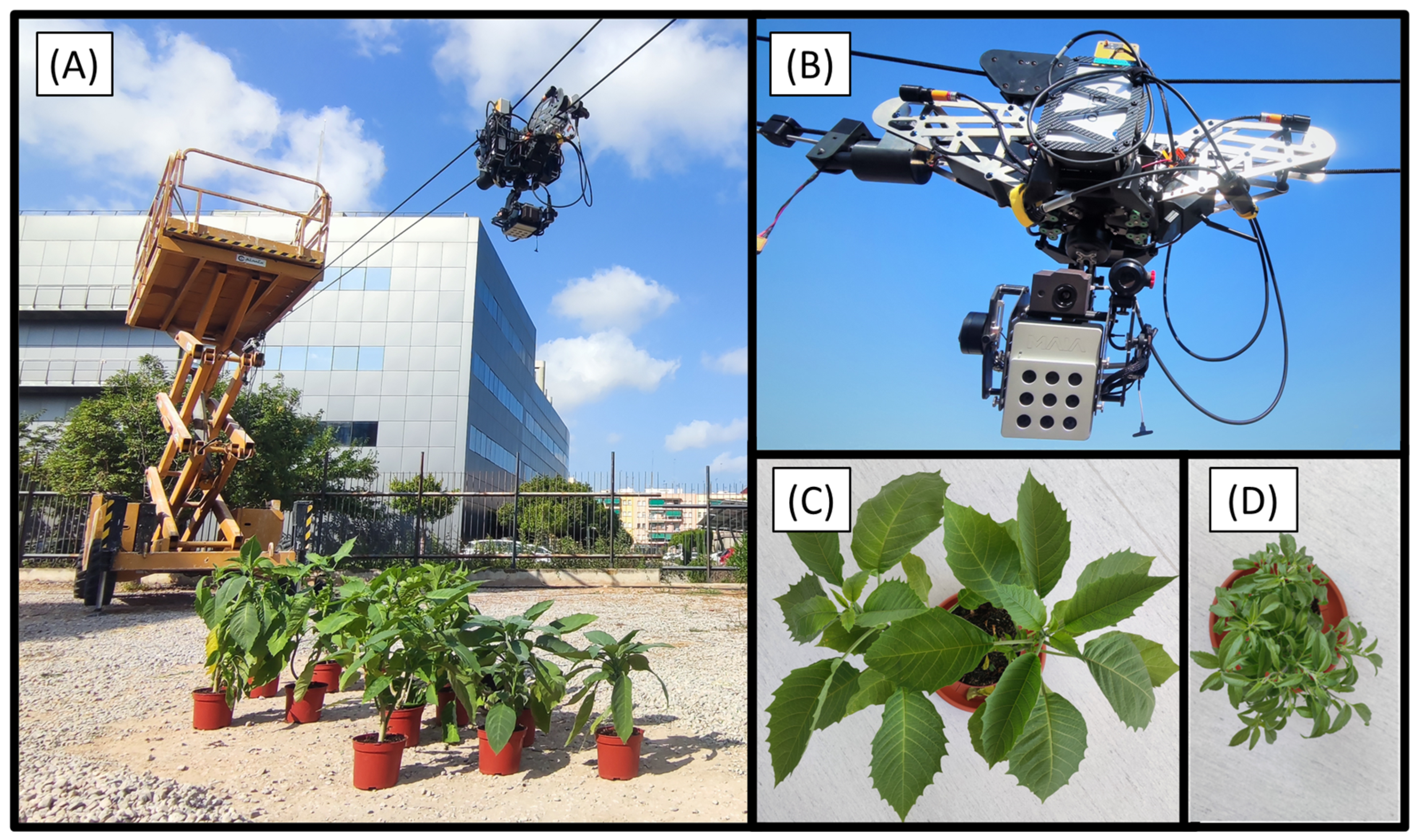
To create a plant canopy experiment with varying levels of vegetation cover, we designed a field experiment based on a transect monitoring of potted plants placed in different densities and patterns. The experiment was conducted at the Parc Científic of the University of Valencia (Paterna, Spain) between 25 and 29 July 2022. The average temperature during the experiment was 30 °C.
We used two species with different canopy architectures based on plant height, leaf size, and distribution. Mealy sage (Salvia farinacea Benth.) was selected as the first plant, which had a dense canopy with a high number of small leaves, approximately 5 cm length. The mealy sage plants (n = 140) were in their first growth stage and had an average height of 30 cm, indicating the first flowering stage. The second plant species, thorn apple (Datura stramonium L.), had a light canopy with few large leaves, measuring approximately 25 cm. The thorn apple plants (n = 15) were in the vegetative stage and had an average height of 50 cm. To avoid drought stress conditions, all plants were watered twice a day before and after the experiment (Figure 1C,D).
Several designs were implemented to create vegetation transects with different levels of vegetation cover. The designs were focused on establishing different transects of either mealy sage or thorn apple, depending on the plant density, on a bare soil surface (Figure 1A). The transect length was approximately 5 m, starting with full plant cover and gradually reducing the plant density towards the end of the transect. The last part of the transect always ended in bare soil. The covered plant area was two metres wide, covered by either 10 plants of mealy sage or 5 plants of thorn apple. Different planting patterns were implemented to mimic different natural layouts with a single species by placing plants in rows or dense blocks on one side of the transect. The main aim was to generate more variability in the proportion of sunlit and shaded canopy due to the shading effect between the plants.

2.2. Multisensor Setup and Transect Sampling Protocol

A multisensor cable-suspended motorized platform (UAV Works, Valencia, Spain) called FluoCat (Figure 1B) was used to monitor the transects in the vegetation area. This platform was specifically designed to measure solar-induced fluorescence and provide additional data for the interpretation of fluorescence emission [36]. It is equipped with the Piccolo Doppio dual spectrometer system (GeoSciences, University of Edinburgh, Edinburgh, UK), a MAIAS2 multispectral camera with the ILS irradiance sensor module (SAL Engineering, Russi, Italy), and a TeAx Thermal Capture Fusion camera (TeAx Technology, Wilnsdorf, Germany), as shown in Figure 2. Two scissor lifts were used 20 m apart to suspend the system over the plant transect using ropes attached to the lifts. The lifts were positioned to ensure a minimum distance of 2.5 m between the sensors and the ground surface.
The Piccolo Doppio (hereafter referred to as Piccolo) is a dual-FOV hyperspectral point system [37], consisting of two QEPro spectroradiometers (Ocean Optics, Dunedin, FL, USA) and a bifurcated fibre optic with shutters to alternately acquire the downwelling solar irradiance (FOV 180°) and the surface upwelling radiance (FOV ~23°) almost instantaneously. With the height setup mentioned above, a ground FOV of at least 1 m was covered. The fibre optics were connected to two spectroradiometers, one covering the entire VNIR spectral range from 400 to 1180 nm, with a spectral resolution of ~1.5 nm, and another (called FLUO) covering the spectral range from 640 to 790 nm, with a spectral resolution of ~0.3 nm. The TOC surface reflectance was calculated for both radiometers using the signal captured from the upwelling and downwelling channels as described in [36]. The VNIR measurement was used to spectrally parameterise the vegetation, and the FLUO was used to retrieve the SIF. Each measurement consisted of 15 repetitions to compensate for instrumental and environmental variability.
The MAIAS2 multispectral camera provided reflectance imagery emulating the first 9 spectral bands of Sentinel-2. The camera had a horizontal field of view of 35° and a vertical field of view of 26°. The images were preprocessed by MultiCam Stitcher Pro v1.4, where the reflectance was calculated from the data measured by the irradiance sensor facing upwards and the images taken with the camera facing downwards. The purpose of MAIA was to extract the spatial distribution of the vegetation measured within the FOV of the Piccolo system as a reference for FVC and FVCsunlit.
A TeAx Thermal Capture Fusion camera was also installed. This is a dual system consisting of two snapshot cameras. The first camera has a thermal sensor covering the long wave infrared (LWIR) range between 7.5 and 13.5 μm with an image resolution of 640 × 512 pixels, a horizontal FOV of 25°, a vertical FOV of 20°, and a thermal resolution of 0.05 K. The second camera is an RGB camera with an image resolution of 1600 × 1200 pixels. This camera was not used in this experiment.
Piccolo’s upwelling channel optics and multispectral and thermal cameras were mounted on a gimbal so that they always pointed down. Piccolo’s downwelling channel optics, equipped with a cosine receptor, and MAIA’s irradiance sensor were mounted so that they always pointed upwards. The projected FOVs of Piccolo and MAIA were calculated to cover the vegetation transect surface with a 0.5 metre buffer zone around the projected FOV area of Piccolo.
The FluoCat was moved along the rope to obtain between 15 and 50 readings for each designed transect. Measurements were taken while the platform was stationary. The average time spent on each transect measurement was approximately 15 min, during which we moved the position of the system in small steps (~10 cm). All instruments on the platform were triggered simultaneously.
The sky conditions during the experiment were generally cloudless, and measurements took place avoiding moments of cloud overpasses.

2.3. Leaf Fluorescence

At the same time as the TOC measurements, reference leaf level measurements were performed in both plant species using a USB4000 radiometer (Ocean Optics, Dunedin, FL, USA) and a FluoWat leaf clip [38]. The FluoWat leaf clip allows the measurement of leaf surface reflectance, transmittance, and up- and downwelling fluorescence. The full chlorophyll fluorescence emission spectrum (650–800 nm) can be obtained by following the protocol in [39].
Sampling consisted of randomly selecting plants of both species from a set of extra pots. The number of leaves sampled each day varied according to the time spent on the TOC measurements. On day 25, 19 leaves were measured (12 from mealy sage, 7 from thorn apple), on day 26, 24 leaves (6 from mealy sage, 14 from thorn apple), on day 27, 6 leaves of thorn apple, and on day 28, 17 leaves (12 from mealy sage, 5 from thorn apple).

2.4. Sunlit Fractional Vegetation Cover Based on MAIA Multispectral Reflectance Images

The MAIA reflectance images were used to obtain the reference total fractional vegetation cover (MAIA FVCtotal) and the reference sunlit fractional vegetation cover (MAIA FVCsunlit) to validate the FVCtotal and FVCsunlit products derived from the Piccolo hyperspectral point spectroradiometer (Section 2.5).
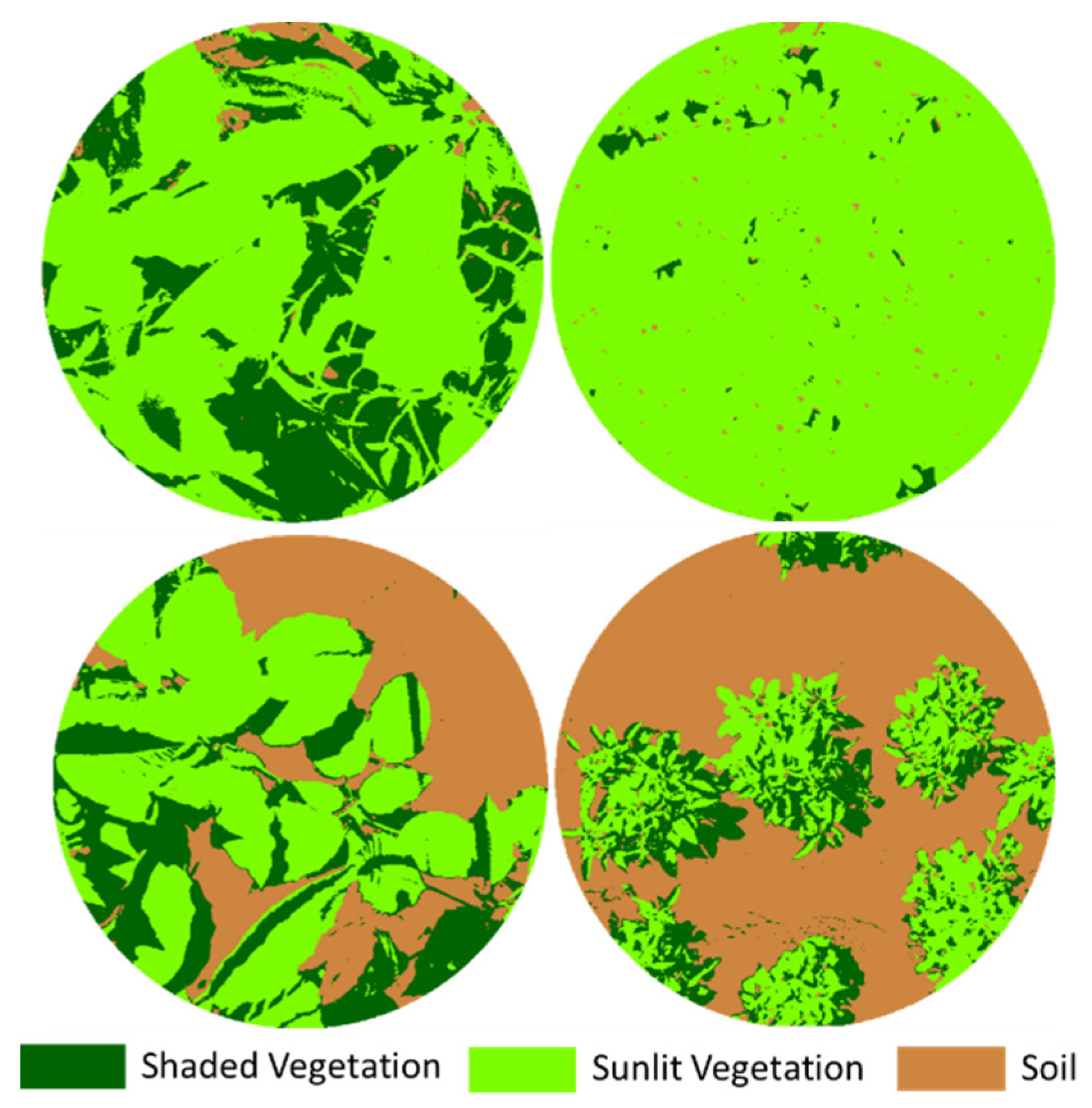
Based on the MAIA’s reflectance images and following the protocol described in [36], we classified each MAIA’s pixel as soil, sunlit, or shaded vegetation fraction. To define the area where the Maia and Piccolo measurements overlapped, the Piccolo FOV was first projected onto the MAIA surface images. To correctly define the coincidence area, the relative position of the optics of the two instruments in the platform gimbal was taken into account (Figure 3). Later, the normalised difference vegetation index (NDVI) was calculated from the reflectance bands 4 and 7 (NDVI = R783 − R665/R783 + R665) [40]. Finally, an NDVI threshold was used to discriminate between soil and vegetation, resulting in the reference MAIA FVCtotal. Based on the MAIA FVCtotal and a reflectance band 7 threshold, a second mask was created to discriminate between sunlit and shaded leaves, resulting in the reference MAIA FVCsunlit and MAIA FVCshaded. For further details see [36].

2.5. Development of Piccolo FVCsunlit Obtained from the TOC Surface Reflectance

2.5.1. Surface Reflectance Unmixing Concept

The spectral response of both vegetation and soil surfaces is mixed in the measured Piccolo VNIR TOC reflectance signal (400–1100 nm). To decompose the fractions of the mixed reflectance signals, the contribution of each element ( i ) was assumed to add linearly to the total surface reflectance, R s u r f a c e   . In order to linearly unmix the surface components, the pure reflectance factors of the sunlit soil and the sunlit and shaded vegetation fractions are required, hereafter referred to as the endmember weights ( w i ). The total TOC surface reflectance is then defined as the sum of n effective reflectance surface components ( R e f f ,   i ), given as the endmember weight ( w i ) times the pure endmember reflectance spectrum ( R i ) ,
R s u r f a c e = i n R e f f ,   i = i n ( w i × R i )
The proposed assumption is based on the decomposition of the surface reflectance ( R s u r f a c e ) into three components associated with the soil, the sunlit vegetation, and the shaded vegetation fractions,
R s u r f a c e = w s o i l × R s o i l + w v e g ,     s u n l i t × R v e g ,   s u n l i t + w v e g ,   s h a d e d × R v e g ,   s h a d e d
By knowing the measured surface endmembers and combining them with a spectral fitting algorithm, it is possible to unravel the abundance of each element. The weights used to combine the endmembers to fit the surface reflectance are understood as the abundance of each endmember. This methodology does not consider the distinction between sunlit and shaded soils, as the spectral feature differences obtained between both types of soils and the white reference with both conditions were lower than 6% across the entire spectrum. This means that the features of the soil spectral signature do not change significantly when the fraction of direct and diffuse light exposition change.

2.5.2. Extraction of Surface Reflectance Endmembers

The proposed unmixing method requires defining three unknown endmembers, these are R s o i l ,     R v e g ,   s u n l i t ,     a n d   R v e g ,   s h a d e d   
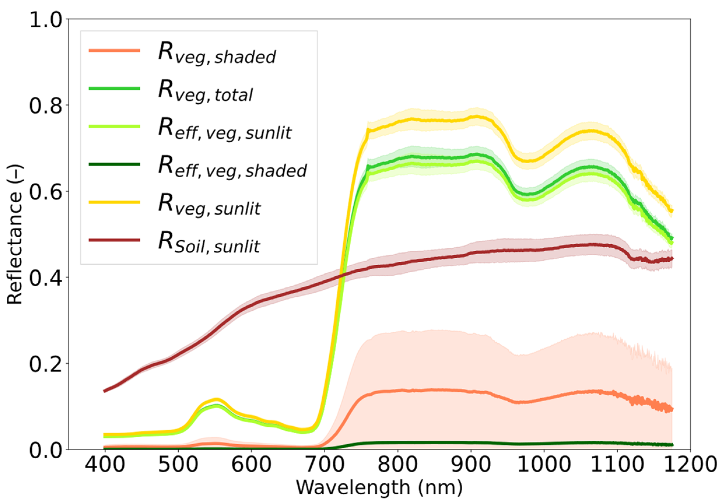
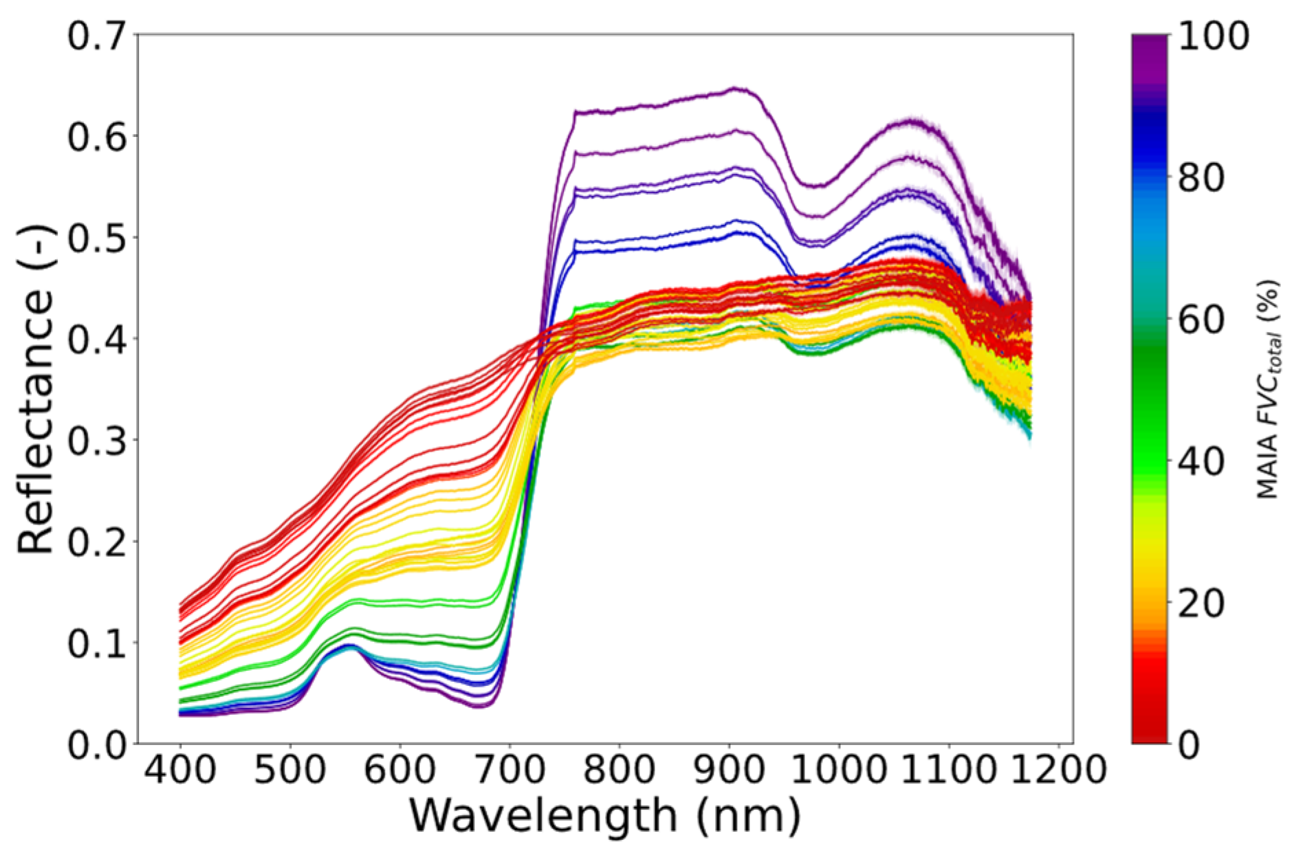
(Equation (2)). Soil, vegetation-sunlit, and vegetation-shaded surfaces were obtained based on MAIA FVC characterization. Reflectance endmembers were defined using ground measurements taken during the experiment with the Piccolo at a 2.5 m height. The R s o i l endmember was obtained from a soil surface where MAIA FVCtotal = 0% (n = 26) (Figure 4, R s o i l ). The pure R v e g ,   s h a d e d endmember was obtained by shielding a vegetation area, MAIA FVCtotal = 100% (n = 1), from direct sunlight with a panel at the side. Regarding R v e g ,   s u n l i t 
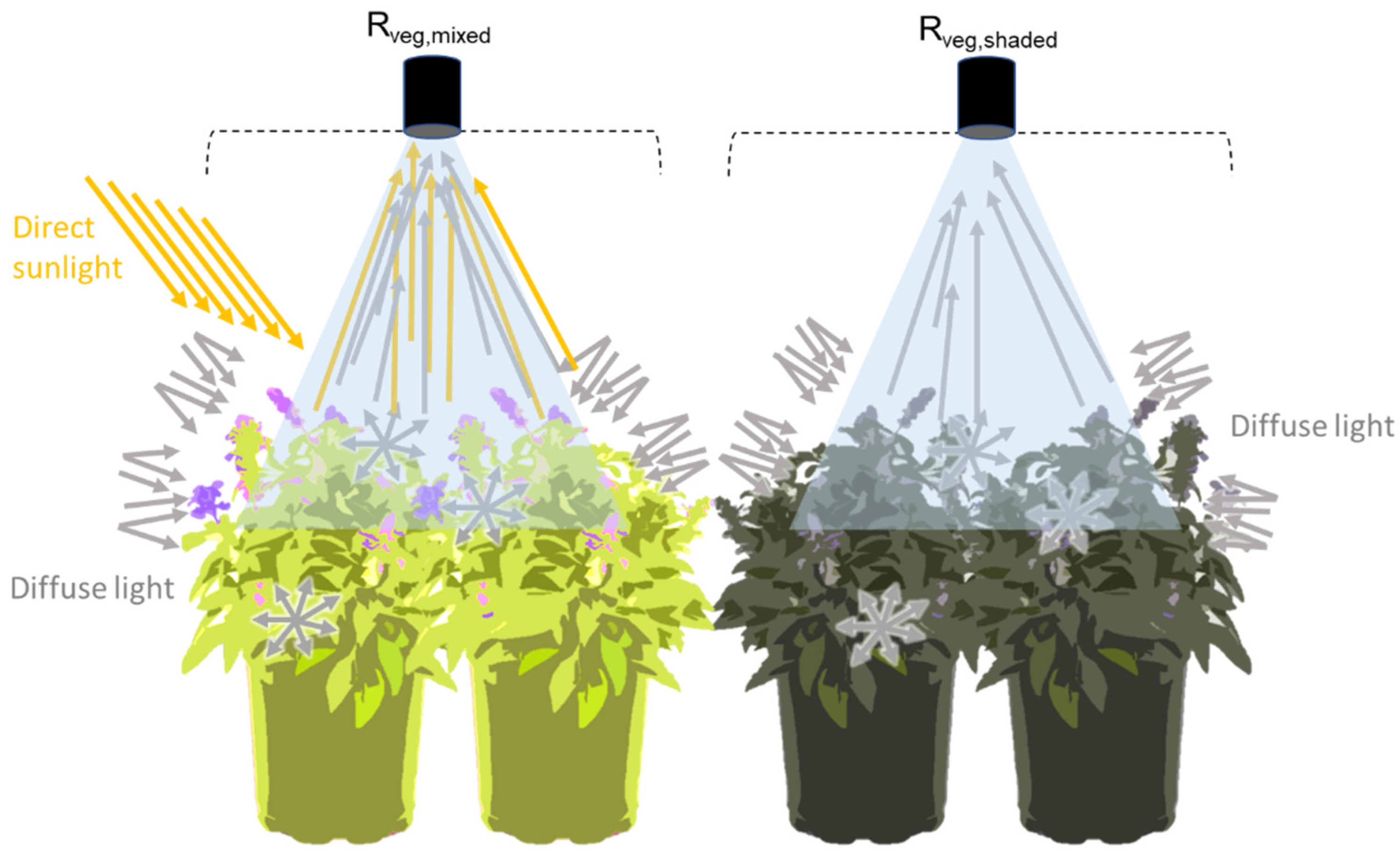
, since it is not possible to measure a spectrum of 100% sunlit vegetation, the strategy was to obtain it indirectly from a TOC total (mixed) vegetation canopy (i.e., sunlit + shaded) and to correct it for the shaded contribution based on the previously obtained R v e g ,   s h a d e d endmember. Furthermore, it must be considered that both the sunlit and total vegetation endmembers are composed of a direct and a diffuse illumination component, while the shaded endmember is composed only of the diffuse component [41]. For simplicity, the potted plants were assumed to have a constant vertical structure (i.e., canopy height, leaf density, and leaf area index). A constant ratio between diffuse and direct components was assumed for the sunlit canopies, and a single diffuse component for the shaded canopies.
TOC mixed vegetation ( R v e g ,   t o t a l ) measurements (assuming that the measured surface is completely covered by vegetation) are defined by the addition of the sunlit and shaded components (Equation (3)),
R v e g ,   t o t a l = w v e g ,   s u n l i t × R v e g , s u n l i t + w v e g , s h a d e d × R v e g , s h a d e d
Moreover, R v e g , s u n l i t is defined as,
R v e g , s u n l i t = 1 n i = 1 n R v e g ,   t o t a l   i w v e g , s h a d e d   ( i ) × R v e g , s h a d e d w v e g ,   s u n l i t   ( i )
where
  • R v e g ,   t o t a l   is the reflectance spectrum of all the Piccolo measurements where MAIA FVCtotal is higher than 95% (n = 16);
  • w v e g ,   s u n l i t and w v e g , s h a d e d are the weight values of sunlit and shaded fractions obtained from the corresponding MAIA reference images, MAIA FVCsunlit, and MAIA FVCshaded, respectively; Section 2.4 (n = 16);
  • R v e g ,   s h a d e d   is the shaded endmember reflectance spectrum previously defined (n = 1).
As the experiment was carried out in summer under high solar illumination angles, the solar sensor target geometry was assumed to have only a minor effect on the distribution and scattering of direct and diffuse light within the canopy. All the endmember spectra used are shown in Figure 4.

2.5.3. Unmixing Strategy

Based on the Piccolo measurements and the reflectance endmembers defined in the previous section, the different fractions of signal components’ contributions (i.e., soil, sunlit vegetation, and shaded vegetation) were unmixed from the surface apparent reflectance using a non-negative least squares (NNLS) fitting (i.e., ‖aXY2, a is the endmember weight and could vary from 0 to 1, X is an m × n matrix (wavelengths × number of endmembers) where X ∈ Rn, and Y ∈ Rm, and Y is the apparent reflectance for each wavelength (m)). Two different approaches were implemented, i.e., approach A, where only soil and mixed vegetation endmembers were considered, and approach B, where three endmembers corresponding to sunlit vegetation, shaded vegetation, and soil were considered. In both cases, the implemented Lawson–Hanson NNLS package in R [42] was used to solve for the contribution (weight and fitted value) of the different signal components. The sum of the estimated weights ( w s o i l   + w v e g , t o t a l or w s o i l   + w v e g ,   s u n l i t +   w v e g ,   s h a d e d )   should be equal to 1. However, in some scenarios, the sum of the weights resulted in values greater than 1. This was proposed to consider other elements present in the scene and the multiple scattering of vegetation, which mainly influences the shaded fraction of vegetation, in the unmixing process [25].
Since the weights represent the vegetation cover fraction, in the next section of the manuscript, we refer to Piccolo FVCtotal, Piccolo FVCsunlit, and Piccolo FVCshaded when referring to the total (i.e., mixed sunlit and shaded), sunlit, and shaded vegetation fractions, respectively. Finally, to validate the unmixing results, for both approaches A and B, the spectral-fitting-based FVC from the Piccolo measurements was compared with the image-based reference FVC of the MAIA measurements by means of the root-mean-square error (RMSE) between the two data pairs (i.e., for approach A: Piccolo FVCtotal vs. Maia FVCtotal and Piccolo FVCtotal vs. Maia FVCsunlit; for approach B: Piccolo FVCtotal vs. Maia FVCtotal, and Piccolo FVCsunlit vs. Maia FVCsunlit).

2.6. TOC Fluorescence Retrieval

Spectrally resolved TOC fluorescence was retrieved using the SpecFit method [43], generating the chlorophyll fluorescence spectrum from 670 to 870 nm. The SpecFit method is based on a weighted spectral fitting method which uses the incoming and surface’s reflected radiance to model the actual reflectance and fluorescence spectra by means of an iterative optimization technique.
From the fluorescence spectrum obtained, the total fluorescence flux J F , t o t a l was calculated based on photon flux units, integrated for the hemisphere, assuming an ideal diffuse scattering behaviour [9] as:
J F , t o t a l p h o t o n s m 2   s 1 = Ω   650 850 J F ,     n a d i r d λ d w   = π   650 850 J F ,     n a d i r d λ

2.7. Retrieval of Piccolo-Based Green APAR Flux of Sunlit Canopy Fraction and Fluorescence Quantum Efficiency

To obtain the sunlit green fluorescence (Equation (6)), also defined as the effective surface fluorescence emission, the green APAR flux of the sunlit canopy fraction ( J A , g r e e n   s u n l i t ) was calculated based on the Piccolo FVCsunlit previously retrieved:
J A , g r e e n   s u n l i t   p h o t o n s m 2   s 1 = A l e a f × P A R × P i c c o l o F V C s u n l i t
where the leaf level absorbance factor (Aleaf) was assumed to be constant at 0.84 [9,44,45], and the PAR was spectrally integrated based on photon flux units obtained from the Piccolo’s downwelling radiance channel. The proposed method assumed that the sunlit fraction was the dominant surface triggering fluorescence emission, and that chlorophyll absorption was constant at the leaf level.
Both the total fluorescence and green sunlit absorbed PAR photon fluxes were then used to calculate the fluorescence quantum efficiency (FQE) as shown by Equation (7).
F Q E = J F , t o t a l   [ μ m o l   m 2 s 1 ] J A , g r e e n   s u n l i t [ μ m o l   m 2 s 1 ]
Further we compared the FQE obtained at the TOC with the FQE values obtained in situ at the leaf level with the FluoWat leaf clip, where the FQE was estimated according to the same formula, considering a FVCsunlit of 1 (i.e., 100% FVCsunlit). The values obtained for each transect were compared with the results at the leaf level made within a time span of 20 min before and after each transect. The transects without leaf measurements in that time range were discarded for the comparison. Two tests were used to compare the pairwise variance of the data from the different scales. Fligner’s test was used to discriminate between different types of data variance. Either Student’s t-test (equal variances) or Welch’s t-test (unequal variances) was used to compare data pairs. All calculations were performed using the Python library Scipy version 1.1 (“PyPI ⋅ The Python Package Index”, 2021).
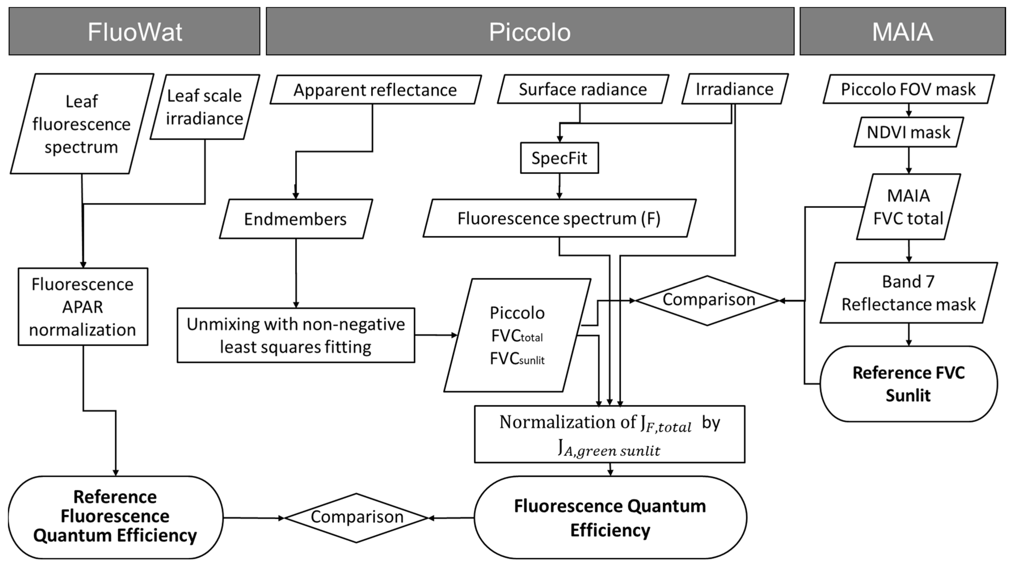
Figure 5 summarises the processing chain applied to obtain the FQE, considering the necessary input parameters and the advanced products obtained due to the sensor’s synergies.

3. Results

3.1. Surface Reflectance and Reference MAIA FVC

In order to test the proposed spectral unmixing method for the spectral retrieval of the fractional vegetation cover, the experiment was designed to obtain a dataset with a full range of fractional vegetation covers from 100% to 0%. A total of 321 surface reflectance measurements were used. Based on the distribution of the reference FVC classifications obtained from the MAIA processing, it can be seen that the full FVC range was covered (Figure 6). The MAIA FVCtotal reference distribution shows, for the range 0–100%, at least 20 measurements for each 10% group, with peaks at both extremes, 0% and 100%, of approximately 45 measurements, and a broad peak of 50 measurements around an FVCtotal of 70%. For the values obtained for the MAIA FVCsunlit and FVCshaded classified fractions, the distribution of the number of measurements shows a higher number of measurements in the 0–10% range for the former and in the 10–20% range for the latter.
Accordingly, the surface reflectance dataset obtained with the spectroradiometer in parallel with the MAIA images from the transect measurements describes a continuous pattern of spectral mixtures between full cover and bare soil surface reflectance. A sample set of transect measured surface reflectance spectra is shown in Figure 7 as a function of the MAIA reference fractional vegetation cover.

3.2. TOC and Leaf Surface Fluorescence

The TOC fluorescence spectra (670–780 nm) obtained by the Specfit retrieval method shows values in an increasing order along the increase in MAIA FVCtotal (Figure 8A). While the fluorescence values around the 740 nm peak show a gradual increase with the MAIA FVCtotal, the fluorescence values at the 687-nm peak remain rather indifferent to the underlying FVC. Interestingly, when FVCtotal = 0–10% (i.e., pure soil), although no fluorescence signal should be obtained, values of the order of 1 mW m−2 sr−1 nm−1 were obtained from the TOC measurements. In terms of magnitude, TOC fluorescence values of the first, rather constant, peak are similar to the leaf level (full surface) values, while the 740 nm peak at the TOC given a FVCtotal = 100% shows values up by a factor of two compared to the leaf value (Figure 8B).

3.3. Surface Reflectance Spectral Unmixing

The proposed surface reflectance unmixing strategies based on two or three endmembers showed slightly different results. In the two-endmember case (approach A), the fitted effective surface reflectance (Reff,surface) was composed of the fitted effective soil and vegetation reflectance (Reff,soil, Reff,veg,total), while for the three-endmember case (approach B), it was composed of the fitted components Reff,soil, Reff,veg,sunlit, and Reff,veg,shade. Figure 9 shows several linear fitting examples of both approaches along a range of MAIA FVCtotal values. In general, the two-endmember unmixing approach slightly overestimated the fitted surface reflectance spectrum, especially in the region beyond the red edge. In contrast, the results from the three-endmember unmixing approach slightly underestimated the fitted reflectance surface spectrum.
For the two strategies, the mean fitting error based on the RMSE between the measured and fitted reflectance, considering all 321 surface reflectance spectra, is shown in Figure 10 (red line). The two-endmember strategy shows a mean fitting error of 0.03 ± 0.02 along the fitted reflectance range while the three-endmember strategy shows a mean fitting error of 0.011 ± 0.007. Using the three-endmember approach resulted in lower fitting errors across the whole spectral range, especially in the NIR region.

3.4. Validation of the Piccolo FVCsunlit Obtained by Spectral Unmixing

Finally, the endmember weights obtained from the surface reflectance unmixing process were used to calculate the spectrally based vegetation cover fractions, which were validated with the MAIA FVCtotal and MAIA FVCsunlit reference products (Figure 11). Generally, for both unmixing approaches, the FVCtotal was underestimated; in contrast, the FVCsunlit fraction was overestimated in comparison with the reference values. The difference between Figure 11A,B in the FVCtotal ranges is due to the fact that no restrictions were applied to the unmixing NNLS weights, resulting in values greater than one when the FVCsunlit and FVCshaded fractions were summed to obtain FVCtotal.
For the two-endmember approach, the RMSE obtained between Piccolo FVCtotal (which integrated sunlit and shaded vegetation) and the MAIA FVCtotal was 0.11, with a coefficient of determination (R2) of 0.88. In addition, the RMSE obtained between Piccolo FVCtotal and the MAIA FVCsunlit was 0.21, with an R2 of 0.86 (Figure 11A). For the three-endmember approach, the Piccolo FVCtotal (obtained by adding the unmixed sunlit and shaded weights) and the Piccolo FVCsunlit were compared with the MAIA FVCtotal and MAIA FVCsunlit, respectively. Compared to the two-endmember approach results, this strategy improved both the correlation factor and the estimated error, with an RMSE between Piccolo FVCtotal and MAIA FVCtotal of 0.13, (R2 = 0.88) and an RMSE between Piccolo FVCsunlit and MAIA FVCsunlit of 0.14, (R2 = 0.84) (Figure 11B).

3.5. Fluorescence Quantum Efficiency

Different examples of the relationships between the retrieved FQE and the calculated green absorbed energy J A , g r e e n   s u n l i t using the three-endmember fitting approach are shown in Figure 12. From these figures, it can be seen that despite the different PAR, APAR, and F fluxes, when the F flux was normalised by the green APAR, similar FQE values were obtained between the samples (FQE ~ 0.4%).
Both the retrieved J A , g r e e n   s u n l i t and TOC fluorescence J F , t o t a l integrated over the spectral range and hemisphere show a clear positive correlation with the fractional vegetation cover (Figure 13A,B,D,E). A higher fractional vegetation cover leads to higher APAR and consequently higher J F , t o t a l values. This relationship becomes stronger when the fluorescence flux is related to the FVCsunlit (R2 = 0.76, Figure 13A,B) compared to FVCtotal (R2 = 0.58, Figure 13D,E). Interestingly, the relationship between FQE, calculated with Equation (7), and FVC shows that FQE remains in the range between 0.3 and 0.8% for FVCsunlit > 20% and FVCtotal > 30% (Figure 13C–F). Within this range, further analyses were carried out on the dataset. These are described below.
Finally, the retrieved FQE at the canopy level was compared to the reference FQE at the leaf level. Only leaf measurements taken 20 min before and after the TOC measurements were included (Figure 14). For this comparison, transects without a leaf reference in the described time range were discarded due to the temporal dynamics of the vegetation. Furthermore, using the values obtained at the leaf level as a reference, TOC measurements with less than 20% of FVCtotal were discarded. Considering these points, TOC FQE values were pooled per transect (average of 18 samples per transect) and compared with the leaf FQE values (average of five samples per transect). From the t-test analysis (p-value = 0.05) of the eleven TOC FQE vs. leaf FQE pairs, only four cases showed statistical differences (25-Salvia 1, 25-Salvia 3, 26-Salvia 1, 28-Datura 1).

4. Discussion

The accurate quantification of the vegetation fluorescence quantum efficiency using remote sensing techniques requires the prior structural characterization of the canopy object acquired in the sensor’s field of view (i.e., point sensor’s field of view and/or imaging sensor’s pixel spatial resolution) [8,10,
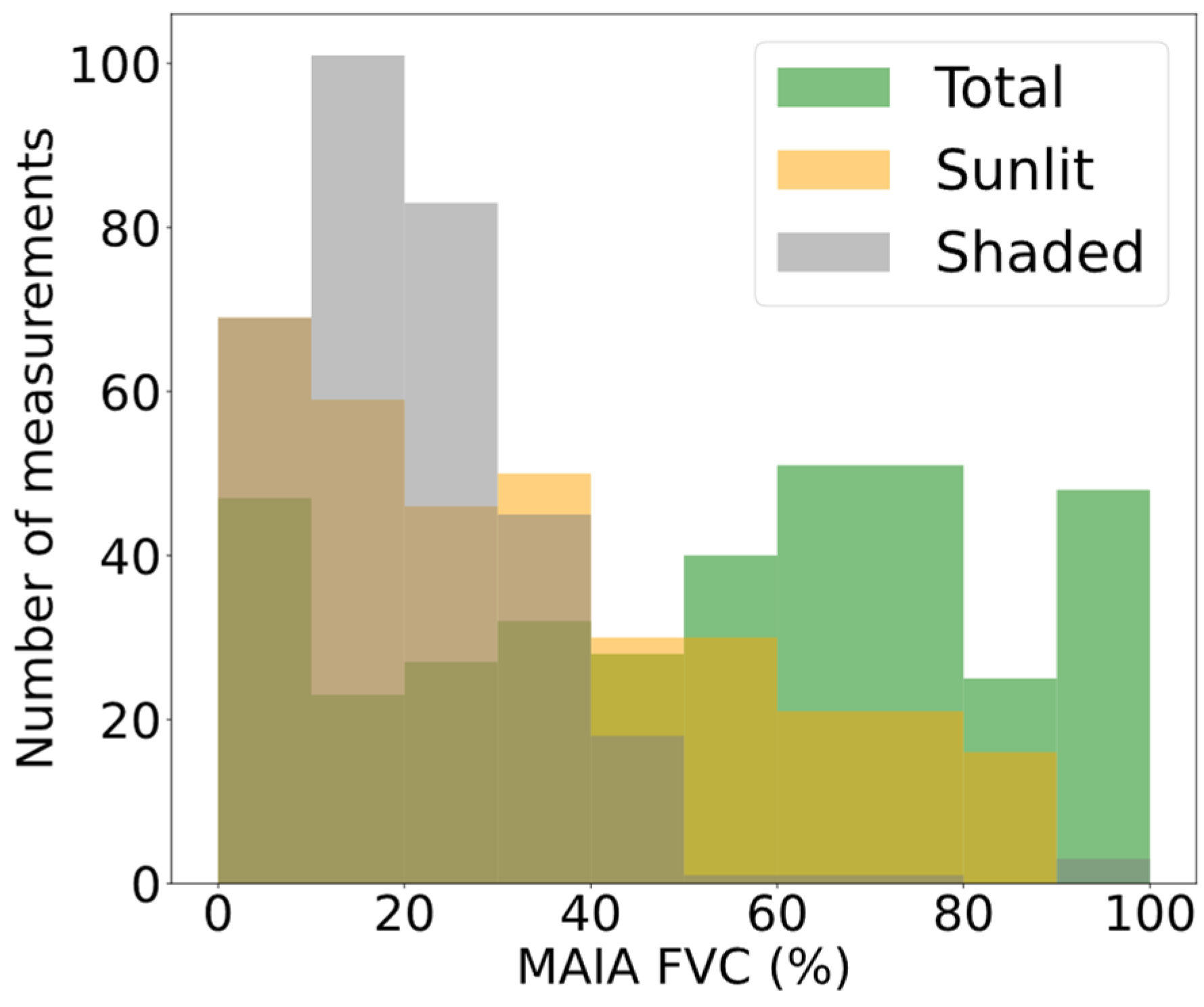
11]. As previously mentioned, this requires the quantification of the amount of incident PAR and APAR, and a correction for the fluorescence scattering and reabsorption within the canopy. In this study, in order to address RQ I, which focuses on disentangling the proportion of sunlit and shaded absorbed PAR, an ad hoc experimental setup was designed to provide a wide range of FVC scenarios by varying the plant density within the sensor FOV, but keeping the vertical vegetation structure constant, thus reducing the variable effect of the canopy scattering and reabsorption. In addition, the use of two plant types with different architectures was used to explore RQ II, assuming that regardless of the FVC and the proportion of sunlit and shaded vegetation, a similar FQE is obtained at the leaf and canopy scales when plants grow under the same environmental conditions. The resulting dataset represented the full range of FVCtotal from 0 to 100% (Figure 6 and Figure 7), having a peak at 70 measurements for 0–10% FVCsunlit and decreasing to 16 measurements for 80% FVCsunlit (Figure 6).
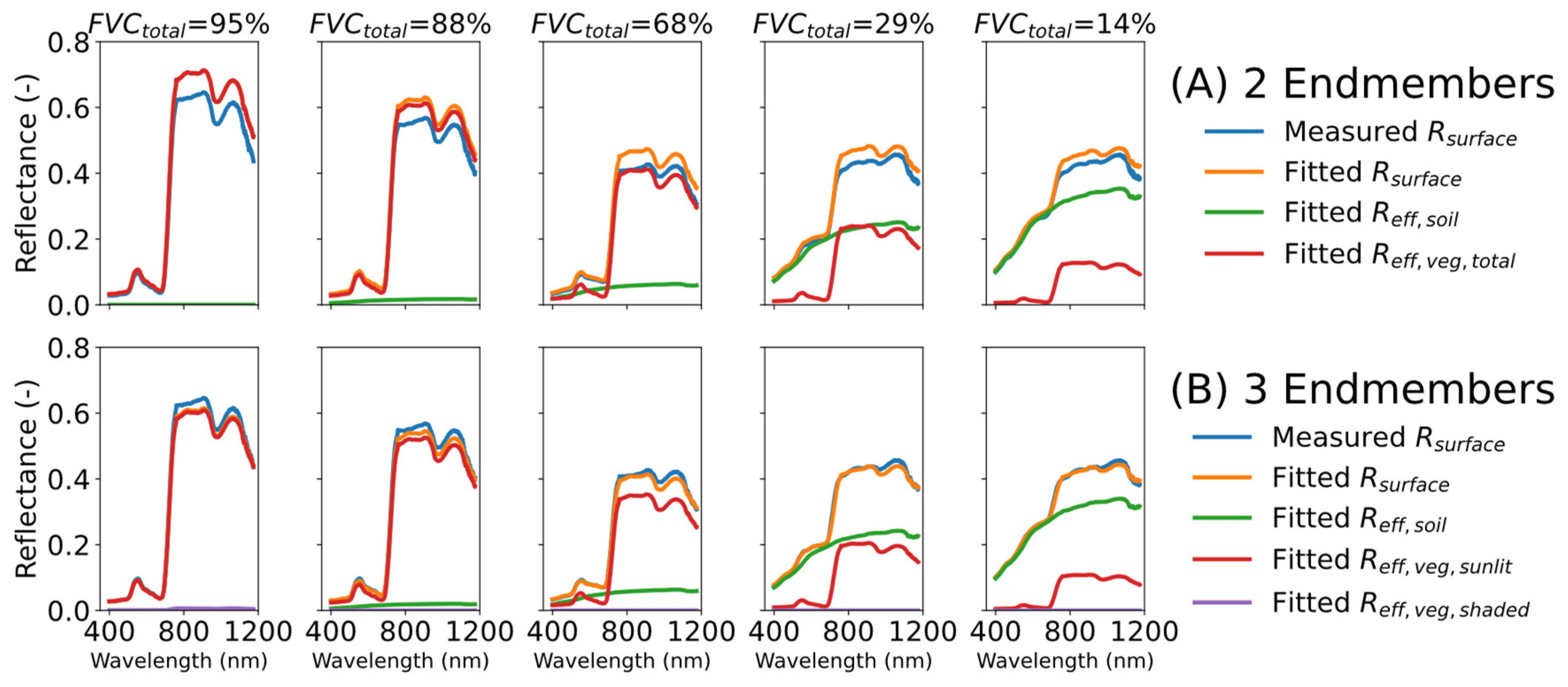
In this study the sunlit and shaded green areas (RQ I) were quantified using a linear unmixing algorithm based on the surface reflectance fitting with specific endmember components. Two different approaches were compared, a two-endmember (Reff,soil, Reff,veg,total, approach A) and a three-endmember (Reff,soil, Reff,veg,sunlit, and R
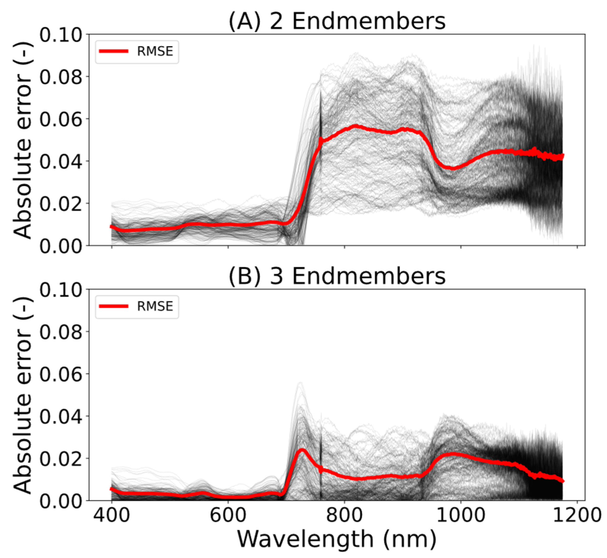
eff,veg,shade, approach B) approach. When comparing the reference and fitted reflectance spectra, the results showed that decomposing the signal using three endmembers provided better results than with two endmembers, reducing the averaged spectral RMSE between the actual reflectance spectrum and the fitted spectrum from 0.03 to 0.01 (Figure 10). The largest difference in terms of RMSE was observed after the red edge, in the NIR range. This can be explained by the nonlinear behaviour of the canopy’s multiple scattering caused by the interaction of the light within the canopy [18]. Moreover, this is the reason why the three-endmembers provided better results than the two-endmember approach. The addition of a shaded vegetation endmember introduced a diffuse component into the fit. This improved the results of the spectral vegetation unmixing in the NIR range in [25].
The fitting accuracy of the presented study is in the same order of magnitude as the results presented in [46,47,48]. These studies, however, reported a higher number of endmembers (e.g., 4–5). For instance, Ref. [47] added to the set of four endmembers (sunlit soil, shaded soil, sunlit vegetation, and shaded vegetation) a fifth endmember with zero reflectance, called photometric shade, which included the multiple scattered signals from the shaded surfaces in the fitting. Their study achieved a maximum RMSE of 0.01 across the optical range. We hypothesise that the reason why our results are consistent with previous studies, despite the use of only three endmembers, is due to the simplicity of the proposed measurement setup, where a reduced number of elements, i.e., flat terrain, homogenous soil surface, and two vegetation structures, define the measured transect. Furthermore, in this study it was not necessary to add a shaded soil endmember because, as assumed by [49], the surface true reflectance was the same, and the differences between sunlit and shaded soil reflectance were mostly due to scattered light from the canopy. Therefore, in the present work, the contribution of the shaded soil was mostly fitted to the shaded vegetation signal, which explains why the addition of FVCsunlit and FVCshaded provided values greater than one.
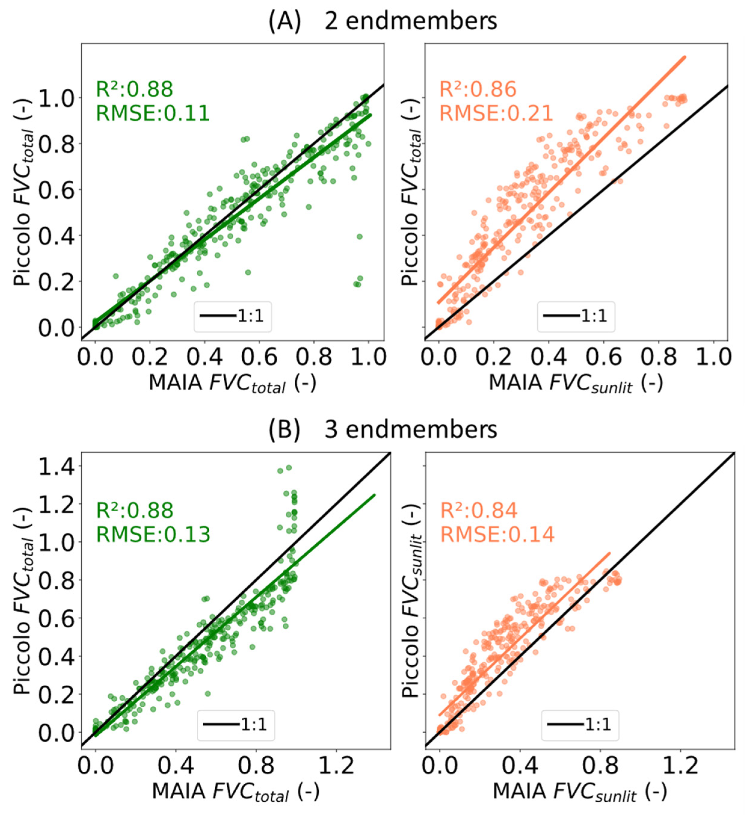
Regarding the discrimination between FVCtotal and FVCsunlit, both the two-endmember and three-endmember approaches provided accurate results when comparing Piccolo FVCtotal and MAIA FVCtotal (R2 = 0.88 and RMSE = 0.11–0.13). However, only the three-endmember approach was able to discriminate between FVCtotal and FVCsunlit, improving the estimation of FVCsunlit (RMSE = 0.14) compared to using the two-endmember approach’s FVCtotal used as an estimation of the sunlit fraction (RMSE = 0.21) (Figure 11). Nevertheless, the results obtained in this study are in the same order of magnitude as other works where more complex hyperspectral unmixing methods have been proposed [50,51,52].
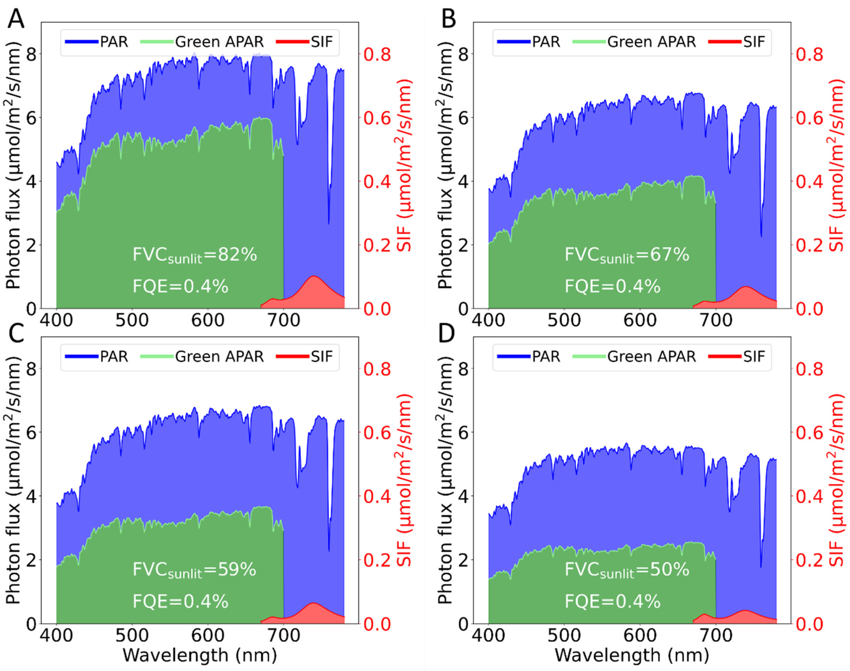
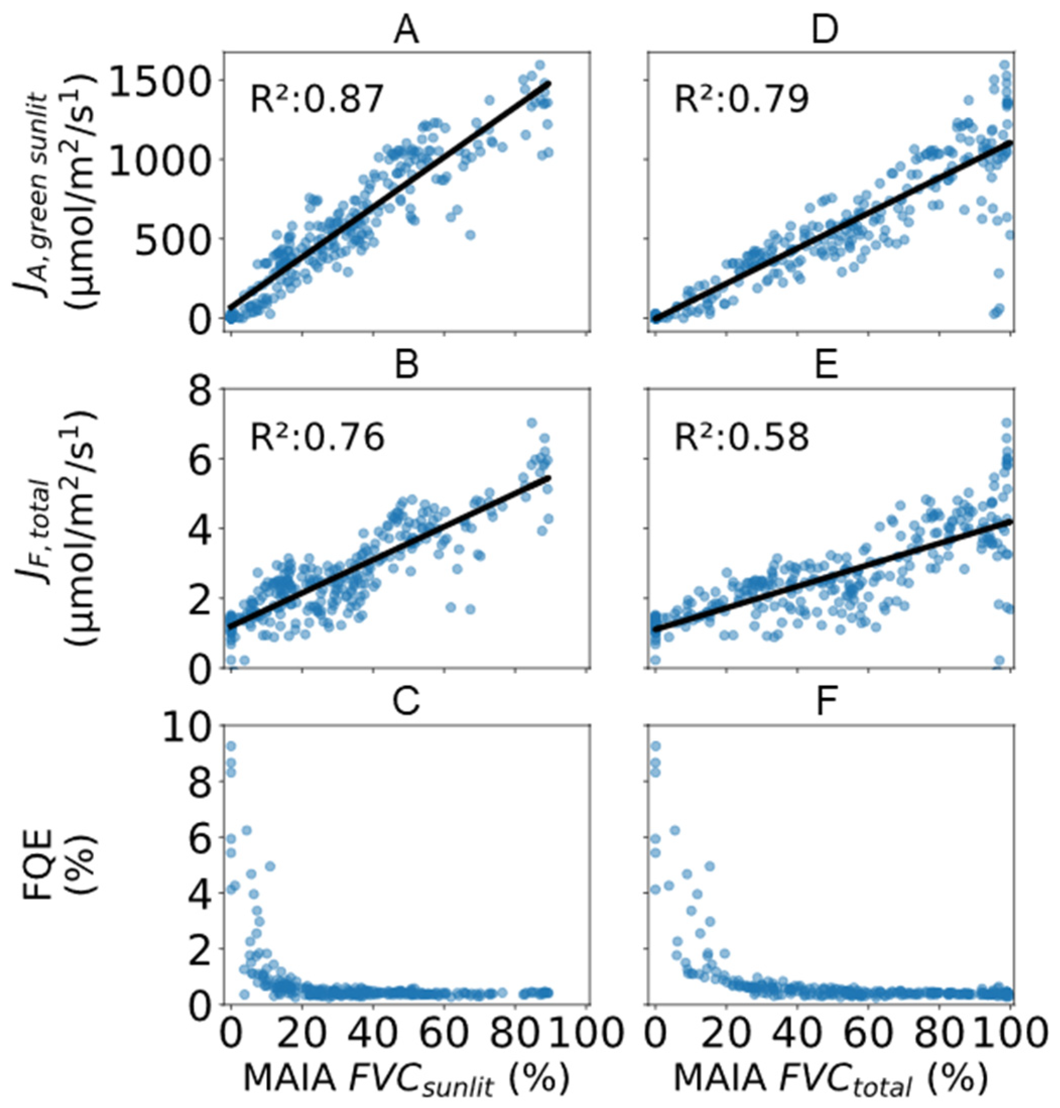
Compared to previous studies where the total (i.e., sunlit + shaded) incoming radiation was estimated using vegetation indices [53,54], the work presented in this study, provides the opportunity to calculate in physical units the actual energy flux arriving at the sunlit photosynthetic surface ( J A , g r e e n   s u n l i t ) (Figure 12A). Furthermore, the results presented in Figure 13B, where the correlation between SIF and MAIA FVCsunlit (R2 = 0.76) is higher than when correlated with FVCtotal (R2 = 0.58), corroborate the hypothesis that the measured TOC SIF is mainly emitted by sunlit leaves [16,17]. Hence, both J A , g r e e n   s u n l i t and the total calculated fluorescence flux ( J F , t o t a l ) show a strong relationship with the FVCsunlit. The combination of these two terms allows us to decouple the changes in J F , t o t a l dynamics driven only by the physiological component [9].
Regarding RQ II, the quantification of the incident APAR and emitted fluorescence photons flux allows the remote quantification of the real fluorescence quantum efficiency (FQE) (Figure 12C). Interestingly, except for FVCsunlit below 20%, similar FQE values were obtained throughout the experiment regardless of the vegetation fractional cover (Figure 12C). These results support the hypothesis that under equal environmental conditions, and without any applied stress such as drought or nitrogen excess/deficit, similar FQE values should be obtained (Figure 13). An accurate estimation of FQE is essential for a quantitative interpretation of SIF and its role in early plant stress detection. Regarding the high FQE values obtained when FVC
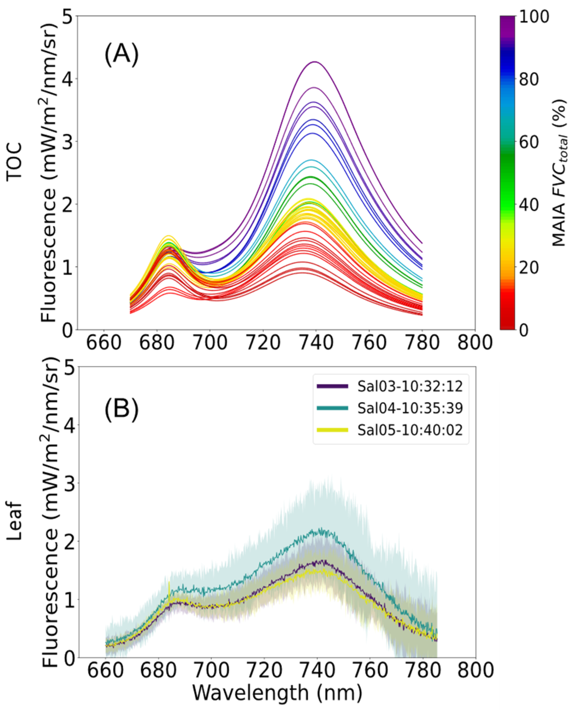
sunlit < 20%, these results could be explained by the positive (and overestimated) SIF values retrieved over samples where bare soil predominates in the measurement transect (Figure 8, red lines). In this study, unfortunately, these observations indicate an overestimation of the retrieved values obtained by the Specfit method in cases with a low FVC. These results are consistent with the findings in [
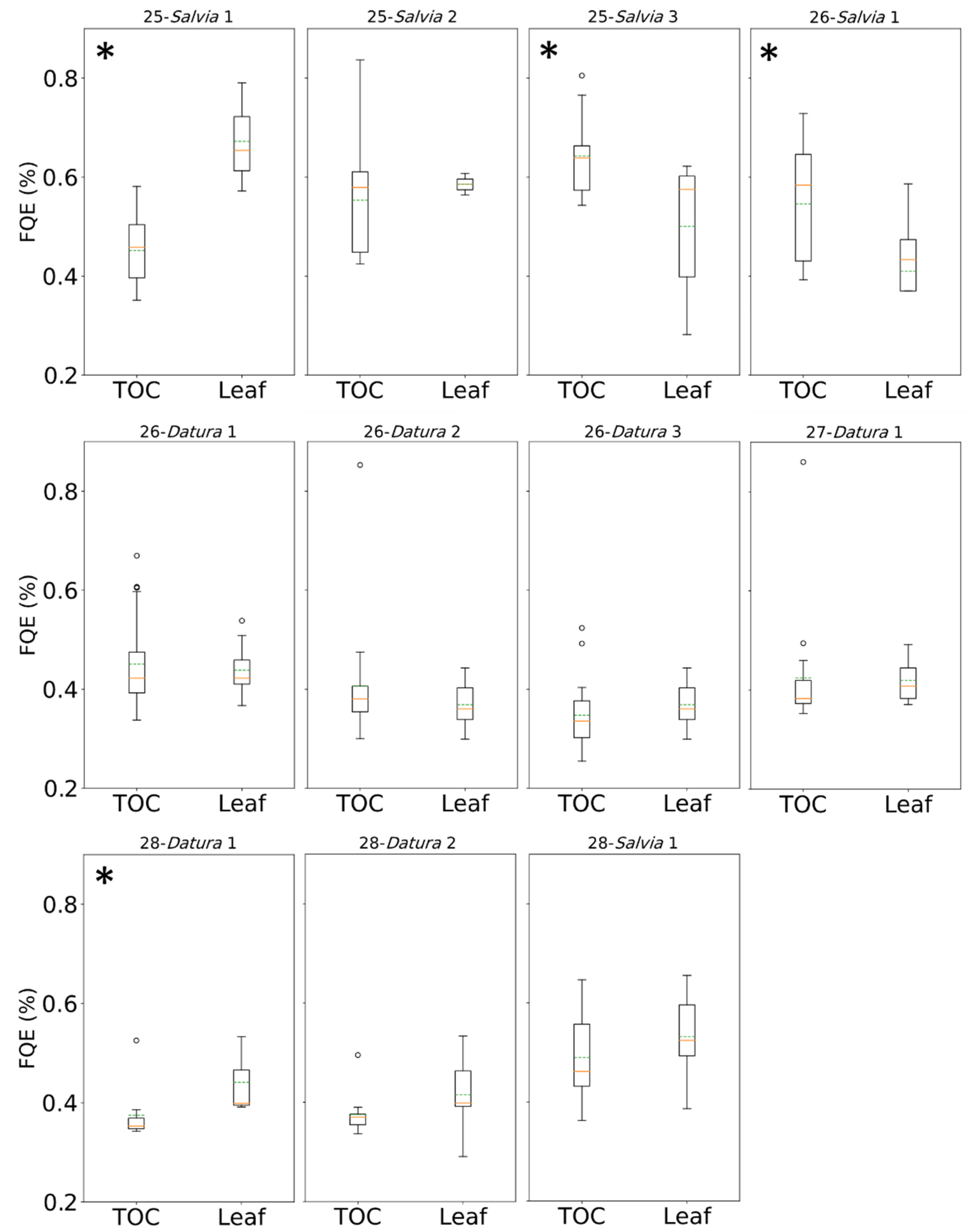
43], where a decrease in performance is observed with a low LAI. These results do not alter the findings of the present study but suggest a revision of the proposed retrieval method when low FVC values are investigated. Consequently, measurements with FVCtotal lower than 20% were discarded for the comparison between TOC and leaf level measurements (Figure 14).
In general terms, the FQE-TOC underestimated the retrieved FQE at the leaf level (Figure 14). In 4 of the 11 transects analysed, the TOC measurements were statistically different from the leaf level measurements. However, despite the slight differences, the FQE obtained at the canopy and leaf levels showed values in the same range and the variability along the experiment was similar. A possible explanation for the differences between them is a combined effect of an overestimation of the fluorescence retrieved, and the omission of the canopy scattering and reabsorption effects when measuring at the TOC due to the light interactions with the canopy [55].
This experiment tested a methodology capable of retrieving the FQE from hyperspectral TOC data, with a protocol to validate the spectral-based FQE values with image-based measurements. However, before extrapolating the proposed methodologies to a larger and more complex ecosystems, further studies are needed to properly characterize and correct for the effects of the canopy’s vertical structure in more heterogeneous surfaces, and to improve the fluorescence retrieval to downscale TOC measurements to the leaf—photosynthetic surface—level. In addition, a further characterization of green (i.e., specific pigment absorption) and nongreen (i.e., woody material and soil absorption libraries) endmembers as well as the atmospheric correction should be incorporated into the proposed methodology. Given the proposed improvements, it is expected that the next studies will apply this methodology to larger scales, such as airborne or satellite measurements, allowing the remote estimation of FQE and consequently the early detection of crop and global vegetation stress.

5. Conclusions

Combining a state-of-the-art set of instruments mounted on a cable-driven platform, this work exploited the synergies between a single-point high-spectral resolution spectroradiometer and a VNIR multispectral imaging camera for reflectance and fluorescence interpretation. This setup allowed the development of an unmixing retrieval scheme to disentangle the fraction of sunlit vegetation cover from the total TOC reflectance, validated by the VNIR imaging camera. By normalising the retrieved TOC fluorescence by the green APAR flux (i.e., sunlit FVC × PAR) the fluorescence quantum yield was quantified. The proposed methodology allows the comparison and validation of the FQE at different scales, from leaf to canopy, with proximal and remote sensors. Furthermore, the methodology presented here, together with the FluoCat system, provides the ability to operate and test similar protocols over large fields, and thus characterize the heterogeneity of the surface, which brings the opportunity to explain/understand the signal measured by the sensor over such an area. In this study, the spectral signature of the sunlit vegetation fraction was used to describe the vegetated surface, which is crucial for Cal/Val activities. From the point of view of the remote sensing methodologies, the quantification of the components present inside the measured area overcomes the limitation of the structural effects on the fluorescence signal, demonstrating that the proposed spectral approach has the potential to unravel the intricate complexities of underlying vegetated surfaces with hyperspectral sensors. The development of more robust methods to obtain products beyond fluorescence, such as the surface effective PAR and APAR, and most importantly the FQE, will allow the remote quantification of the vegetation energy balance, closing the gap between the flux of photons absorbed, dissipated, and used for photochemistry, which is critical for a remote quantification of photosynthesis. Future research lines are needed to investigate the extrapolation of this method to larger scales, with the aim of studying the FQE’s temporal dynamics and variable stress conditions for a global monitoring of vegetation using orbiting satellites.

Author Contributions

Conceptualization, A.M.-E., S.V.W. and M.P.C.-M.; methodology, A.M.-E., S.V.W. and M.P.C.-M.; software, M.A. and S.C.; validation, A.M.-E., S.V.W. and M.P.C.-M.; formal analysis, A.M.-E., S.V.W., M.P.C.-M. and J.M.; investigation, A.M.-E., S.V.W. and M.P.C.-M.; data curation, A.M.-E.; writing—original draft preparation, A.M.-E., S.V.W. and M.P.C.-M.; writing—review and editing, A.M.-E., S.V.W., M.P.C.-M. and J.M.; supervision, J.M.; project administration, J.M. and S.V.W.; funding acquisition, J.M. and S.V.W. All authors have read and agreed to the published version of the manuscript.

Funding

AM was funded by AVANFLEX project (Advanced Products for the FLEX mission), n_ ESP2016-79503-C2-1-P, Ministry of Economy and Competitiveness, Spain. SVW, MPC, and AM are currently funded by European Research Council (ERC) under the ERC-2021-STG PHOTOFLUX project (grant agreement 101041768). The instruments were funded by European Regional Development Fund (no. IDIFEDER/2018/050).

Data Availability Statement

The data presented in this study are available on request from the corresponding author.

Acknowledgments

The authors would like to thank Laura Mihai for the Piccolo calibration and validation conducted during the experiment.

Conflicts of Interest

The authors declare no conflict of interest. The funders had no role in the design of the study; in the collection, analyses, or interpretation of data; in the writing of the manuscript; or in the decision to publish the results.

References

  1. Drusch, M.; Moreno, J.; Del Bello, U.; Franco, R.; Goulas, Y.; Huth, A.; Kraft, S.; Middleton, E.M.; Miglietta, F.; Mohammed, G.; et al. The FLuorescence EXplorer Mission Concept-ESA’s Earth Explorer 8. IEEE Trans. Geosci. Remote Sens. 2017, 55, 1273–1284. [Google Scholar] [CrossRef]
  2. Buschmann, C. Variability and Application of the Chlorophyll Fluorescence Emission Ratio Red/Far-Red of Leaves. Photosynth. Res. 2007, 92, 261–271. [Google Scholar] [CrossRef]
  3. Franck, F.; Juneau, P.; Popovic, R. Resolution of the Photosystem I and Photosystem II Contributions to Chlorophyll Fluorescence of Intact Leaves at Room Temperature. Biochim. Et. Biophys. Acta (BBA) Bioenerg. 2002, 1556, 239–246. [Google Scholar] [CrossRef]
  4. Jin, C.; Zha, T.; Bourque, C.P.-A.; Liu, P.; Jia, X.; Tian, Y.; Li, X.; Liu, X.; Guo, X.; Xu, M.; et al. Key Stress Indicators from Chlorophyll Fluorescence in Five Desert Plant Species. Ecol. Indic. 2022, 145, 109679. [Google Scholar] [CrossRef]
  5. Magney, T.S.; Frankenberg, C.; Köhler, P.; North, G.; Davis, T.S.; Dold, C.; Dutta, D.; Fisher, J.B.; Grossmann, K.; Harrington, A.; et al. Disentangling Changes in the Spectral Shape of Chlorophyll Fluorescence: Implications for Remote Sensing of Photosynthesis. J. Geophys. Res. Biogeosciences 2019, 124, 1491–1507. [Google Scholar] [CrossRef]
  6. Maxwell, K.; Johnson, G.N. Chlorophyll Fluorescence—A Practical Guide. J. Exp. Bot. 2000, 51, 659–668. [Google Scholar] [CrossRef]
  7. Alonso, L.; Van Wittenberghe, S.; Amorós-López, J.; Vila-Francés, J.; Gómez-Chova, L.; Moreno, J. Diurnal Cycle Relationships between Passive Fluorescence, PRI and NPQ of Vegetation in a Controlled Stress Experiment. Remote Sens. 2017, 9, 770. [Google Scholar] [CrossRef]
  8. Regaieg, O.; Yin, T.; Malenovský, Z.; Cook, B.D.; Morton, D.C.; Gastellu-Etchegorry, J.-P. Assessing Impacts of Canopy 3D Structure on Chlorophyll Fluorescence Radiance and Radiative Budget of Deciduous Forest Stands Using DART. Remote Sens. Environ. 2021, 265, 112673. [Google Scholar] [CrossRef]
  9. Van Wittenberghe, S.; Sabater, N.; Cendrero-Mateo, M.P.; Tenjo, C.; Moncholi, A.; Alonso, L.; Moreno, J. Towards the Quantitative and Physically-Based Interpretation of Solar-Induced Vegetation Fluorescence Retrieved from Global Imaging. Photosynthetica 2021, 59, 438–457. [Google Scholar] [CrossRef]
  10. Yang, P.; van der Tol, C.; Verhoef, W.; Damm, A.; Schickling, A.; Kraska, T.; Muller, O.; Rascher, U. Using Reflectance to Explain Vegetation Biochemical and Structural Effects on Sun-Induced Chlorophyll Fluorescence. Remote Sens. Environ. 2019, 231, 110996. [Google Scholar] [CrossRef]
  11. Zhang, X.; Zhang, Z.; Zhang, Y.; Zhang, Q.; Liu, X.; Chen, J.; Wu, Y.; Wu, L. Influences of Fractional Vegetation Cover on the Spatial Variability of Canopy SIF from Unmanned Aerial Vehicle Observations. Int. J. Appl. Earth Obs. Geoinf. 2022, 107, 102712. [Google Scholar] [CrossRef]
  12. Oguchi, R.; Hikosaka, K.; Hirose, T. Does the Photosynthetic Light-Acclimation Need Change in Leaf Anatomy? Plant Cell Environ. 2003, 26, 505–512. [Google Scholar] [CrossRef]
  13. Moncholi-Estornell, A.; Van Wittenberghe, S.; Cendrero-Mateo, M.P.; Alonso, L.; Malenovský, Z.; Moreno, J. Impact of Structural, Photochemical and Instrumental Effects on Leaf and Canopy Reflectance Variability in the 500–600 Nm Range. Remote Sens. 2022, 14, 56. [Google Scholar] [CrossRef]
  14. Porcar-Castell, A.; Malenovský, Z.; Magney, T.; Van Wittenberghe, S.; Fernández-Marín, B.; Maignan, F.; Zhang, Y.; Maseyk, K.; Atherton, J.; Albert, L.P.; et al. Chlorophyll a Fluorescence Illuminates a Path Connecting Plant Molecular Biology to Earth-System Science. Nat. Plants 2021, 7, 998–1009. [Google Scholar] [CrossRef] [PubMed]
  15. Verrelst, J.; Rivera, J.P.; van der Tol, C.; Magnani, F.; Mohammed, G.; Moreno, J. Global Sensitivity Analysis of the SCOPE Model: What Drives Simulated Canopy-Leaving Sun-Induced Fluorescence? Remote Sens. Environ. 2015, 166, 8–21. [Google Scholar] [CrossRef]
  16. Biriukova, K.; Celesti, M.; Evdokimov, A.; Pacheco-Labrador, J.; Julitta, T.; Migliavacca, M.; Giardino, C.; Miglietta, F.; Colombo, R.; Panigada, C.; et al. Effects of Varying Solar-View Geometry and Canopy Structure on Solar-Induced Chlorophyll Fluorescence and PRI. Int. J. Appl. Earth Obs. Geoinf. 2020, 89, 102069. [Google Scholar] [CrossRef]
  17. Pinto, F.; Müller-Linow, M.; Schickling, A.; Cendrero-Mateo, M.P.; Ballvora, A.; Rascher, U. Multiangular Observation of Canopy Sun-Induced Chlorophyll Fluorescence by Combining Imaging Spectroscopy and Stereoscopy. Remote Sens. 2017, 9, 415. [Google Scholar] [CrossRef]
  18. García-Haro, F.J.; Camacho, F.; Martínez, B.; Campos-Taberner, M.; Fuster, B.; Sánchez-Zapero, J.; Gilabert, M.A. Climate Data Records of Vegetation Variables from Geostationary SEVIRI/MSG Data: Products, Algorithms and Applications. Remote Sens. 2019, 11, 2103. [Google Scholar] [CrossRef]
  19. Li, L.; Mu, X.; Jiang, H.; Chianucci, F.; Hu, R.; Song, W.; Qi, J.; Liu, S.; Zhou, J.; Chen, L.; et al. Review of Ground and Aerial Methods for Vegetation Cover Fraction (FCover) and Related Quantities Estimation: Definitions, Advances, Challenges, and Future Perspectives. ISPRS J. Photogramm. Remote Sens. 2023, 199, 133–156. [Google Scholar] [CrossRef]
  20. Zhang, C.; Ma, L.; Chen, J.; Rao, Y.; Zhou, Y.; Chen, X. Assessing the Impact of Endmember Variability on Linear Spectral Mixture Analysis (LSMA): A Theoretical and Simulation Analysis. Remote Sens. Environ. 2019, 235, 111471. [Google Scholar] [CrossRef]
  21. Asner, G.P.; Heidebrecht, K.B. Spectral Unmixing of Vegetation, Soil and Dry Carbon Cover in Arid Regions: Comparing Multispectral and Hyperspectral Observations. Int. J. Remote Sens. 2002, 23, 3939–3958. [Google Scholar] [CrossRef]
  22. Baret, F.; Weiss, M.; Lacaze, R.; Camacho, F.; Makhmara, H.; Pacholcyzk, P.; Smets, B. GEOV1: LAI and FAPAR Essential Climate Variables and FCOVER Global Time Series Capitalizing over Existing Products. Part1: Principles of Development and Production. Remote Sens. Environ. 2013, 137, 299–309. [Google Scholar] [CrossRef]
  23. Hu, P.; Chapman, S.C.; Zheng, B.; Hu, P.; Chapman, S.C.; Zheng, B. Coupling of Machine Learning Methods to Improve Estimation of Ground Coverage from Unmanned Aerial Vehicle (UAV) Imagery for High-Throughput Phenotyping of Crops. Funct. Plant Biol. 2021, 48, 766–779. [Google Scholar] [CrossRef] [PubMed]
  24. Johnson, P.E.; Smith, M.O.; Taylor-George, S.; Adams, J.B. A Semiempirical Method for Analysis of the Reflectance Spectra of Binary Mineral Mixtures. J. Geophys. Res. Solid. Earth 1983, 88, 3557–3561. [Google Scholar] [CrossRef]
  25. Roberts, D.A.; Smith, M.O.; Adams, J.B. Green Vegetation, Nonphotosynthetic Vegetation, and Soils in AVIRIS Data. Remote Sens. Environ. 1993, 44, 255–269. [Google Scholar] [CrossRef]
  26. Chen, J.M.; Leblanc, S.G. A Four-Scale Bidirectional Reflectance Model Based on Canopy Architecture. IEEE Trans. Geosci. Remote Sens. 1997, 35, 1316–1337. [Google Scholar] [CrossRef]
  27. Wang, X.; Zheng, G.; Yun, Z.; Xu, Z.; Moskal, L.M.; Tian, Q. Characterizing the Spatial Variations of Forest Sunlit and Shaded Components Using Discrete Aerial Lidar. Remote Sens. 2020, 12, 1071. [Google Scholar] [CrossRef]
  28. Zhang, Q.; Chen, J.M.; Ju, W.; Wang, H.; Qiu, F.; Yang, F.; Fan, W.; Huang, Q.; Wang, Y.; Feng, Y.; et al. Improving the Ability of the Photochemical Reflectance Index to Track Canopy Light Use Efficiency through Differentiating Sunlit and Shaded Leaves. Remote Sens. Environ. 2017, 194, 1–15. [Google Scholar] [CrossRef]
  29. Zheng, T.; Chen, J.M. Photochemical Reflectance Ratio for Tracking Light Use Efficiency for Sunlit Leaves in Two Forest Types. ISPRS J. Photogramm. Remote Sens. 2017, 123, 47–61. [Google Scholar] [CrossRef]
  30. Adams, J.B.; Sabol, D.E.; Kapos, V.; Almeida Filho, R.; Roberts, D.A.; Smith, M.O.; Gillespie, A.R. Classification of Multispectral Images Based on Fractions of Endmembers: Application to Land-Cover Change in the Brazilian Amazon. Remote Sens. Environ. 1995, 52, 137–154. [Google Scholar] [CrossRef]
  31. Bartholomeus, H.; Kooistra, L.; Stevens, A.; van Leeuwen, M.; van Wesemael, B.; Ben-Dor, E.; Tychon, B. Soil Organic Carbon Mapping of Partially Vegetated Agricultural Fields with Imaging Spectroscopy. Int. J. Appl. Earth Obs. Geoinf. 2011, 13, 81–88. [Google Scholar] [CrossRef]
  32. Liu, Y.; Pan, X.-Z.; Shi, R.-J.; Li, Y.-L.; Wang, C.-K.; Li, Z.-T. Predicting Soil Salt Content Over Partially Vegetated Surfaces Using Non-Negative Matrix Factorization. IEEE J. Sel. Top. Appl. Earth Obs. Remote Sens. 2015, 8, 5305–5316. [Google Scholar] [CrossRef]
  33. Li, Y.; Liu, Y.; Wu, S.; Wang, C.; Xu, A.; Pan, X. Hyper-Spectral Estimation of Wheat Biomass after Alleviating of Soil Effects on Spectra by Non-Negative Matrix Factorization. Eur. J. Agron. 2017, 84, 58–66. [Google Scholar] [CrossRef]
  34. Dechant, B.; Ryu, Y.; Badgley, G.; Zeng, Y.; Berry, J.A.; Zhang, Y.; Goulas, Y.; Li, Z.; Zhang, Q.; Kang, M.; et al. Canopy Structure Explains the Relationship between Photosynthesis and Sun-Induced Chlorophyll Fluorescence in Crops. Remote Sens. Environ. 2020, 241, 111733. [Google Scholar] [CrossRef]
  35. Moreno, J.F. Advances in the Retrieval and Interpretation of Solar-Induced Vegetation Chlorophyll Fluorescence Using Passive Remote Sensing Techniques. In Proceedings of the 2021 IEEE International Geoscience and Remote Sensing Symposium IGARSS, Brussels, Belgium, 11–16 July 2021; pp. 1915–1918. [Google Scholar]
  36. Moncholi-Estornell, A.; Van Wittenberghe, S.; Pilar Cendrero-Mateo, M.; Alonso, L.; Jiménez, M.; Urrego, P.; Mac Arthur, A.; Moreno, J. FluoCat: A Cable-Suspended Multi-Sensor System for the Vegetation SIF Cal/Val Monitoring and Estimation of Effective Sunlit Surface Fluorescence. Int. J. Appl. Earth Obs. Geoinf. 2023, 116, 103147. [Google Scholar] [CrossRef]
  37. Mac Arthur, A.; Robinson, I. A Critique of Field Spectroscopy and the Challenges and Opportunities It Presents for Remote Sensing for Agriculture, Ecosystems, and Hydrology. In Proceedings of the Remote Sensing for Agriculture, Ecosystems, and Hydrology XVII, Toulouse, France, 22–24 September 2015; SPIE: Bellingham, WA, USA; Volume 9637, pp. 29–39. [Google Scholar]
  38. Alonso, L. Passive Direct Measurement of Sun-Induced Chlorophyll Fluorescence Spectrum from in Vivo Leaves. Doctoral Thesis, Universitat de València, Valencia, Spain, 2022. [Google Scholar]
  39. Van Wittenberghe, S.; Alonso, L.; Verrelst, J.; Hermans, I.; Delegido, J.; Veroustraete, F.; Valcke, R.; Moreno, J.; Samson, R. Upward and Downward Solar-Induced Chlorophyll Fluorescence Yield Indices of Four Tree Species as Indicators of Traffic Pollution in Valencia. Environ. Pollut. 2013, 173, 29–37. [Google Scholar] [CrossRef]
  40. Rouse, J.W.; Haas, R.H.; Schell, J.A.; Deering, D.W. Monitoring Vegetation Systems in the Great Plains with ERTS. NASA Spec. Publ. 1974, 351, 309. [Google Scholar]
  41. Wilson, J.W. Stand Structure and Light Penetration. III. Sunlit Foliage Area. J. Appl. Ecol. 1967, 4, 159–165. [Google Scholar] [CrossRef]
  42. Mullen, K.M.; van Stokkum, I.H.M. nnls: The Lawson-Hanson Algorithm for Non-Negative Least Squares (NNLS). R Package Version 1.4. 2012. Available online: https://CRAN.R-project.org/package=nnls (accessed on 28 August 2023).
  43. Cogliati, S.; Celesti, M.; Cesana, I.; Miglietta, F.; Genesio, L.; Julitta, T.; Schuettemeyer, D.; Drusch, M.; Rascher, U.; Jurado, P.; et al. A Spectral Fitting Algorithm to Retrieve the Fluorescence Spectrum from Canopy Radiance. Remote Sens. 2019, 11, 1840. [Google Scholar] [CrossRef]
  44. Baker, N.R. Chlorophyll Fluorescence: A Probe of Photosynthesis In Vivo. Annu. Rev. Plant Biol. 2008, 59, 89–113. [Google Scholar] [CrossRef]
  45. Björkman, O.; Demmig, B. Photon Yield of O2 Evolution and Chlorophyll Fluorescence Characteristics at 77 K among Vascular Plants of Diverse Origins. Planta 1987, 170, 489–504. [Google Scholar] [CrossRef]
  46. Cunnick, H.; Ramage, J.M.; Magness, D.; Peters, S.C. Mapping Fractional Vegetation Coverage across Wetland Classes of Sub-Arctic Peatlands Using Combined Partial Least Squares Regression and Multiple Endmember Spectral Unmixing. Remote Sens. 2023, 15, 1440. [Google Scholar] [CrossRef]
  47. Fitzgerald, G.J.; Pinter, P.J.; Hunsaker, D.J.; Clarke, T.R. Multiple Shadow Fractions in Spectral Mixture Analysis of a Cotton Canopy. Remote Sens. Environ. 2005, 97, 526–539. [Google Scholar] [CrossRef]
  48. .Miao, Y.; Yang, B. Multilevel Reweighted Sparse Hyperspectral Unmixing Using Superpixel Segmentation and Particle Swarm Optimization. IEEE Geosci. Remote Sens. Lett. 2022, 19, 1–5. [Google Scholar] [CrossRef]
  49. Markiet, V.; Mõttus, M. Estimation of Boreal Forest Floor Reflectance from Airborne Hyperspectral Data of Coniferous Forests. Remote Sens. Environ. 2020, 249, 112018. [Google Scholar] [CrossRef]
  50. Dennison, P.E.; Qi, Y.; Meerdink, S.K.; Kokaly, R.F.; Thompson, D.R.; Daughtry, C.S.T.; Quemada, M.; Roberts, D.A.; Gader, P.D.; Wetherley, E.B.; et al. Comparison of Methods for Modeling Fractional Cover Using Simulated Satellite Hyperspectral Imager Spectra. Remote Sens. 2019, 11, 2072. [Google Scholar] [CrossRef]
  51. Fernández-Guisuraga, J.M.; Calvo, L.; Suárez-Seoane, S. Comparison of Pixel Unmixing Models in the Evaluation of Post-Fire Forest Resilience Based on Temporal Series of Satellite Imagery at Moderate and Very High Spatial Resolution. ISPRS J. Photogramm. Remote Sens. 2020, 164, 217–228. [Google Scholar] [CrossRef]
  52. Ma, Y.; Jin, Q.; Mei, X.; Dai, X.; Fan, F.; Li, H.; Huang, J. Hyperspectral Unmixing with Gaussian Mixture Model and Low-Rank Representation. Remote Sens. 2019, 11, 911. [Google Scholar] [CrossRef]
  53. Dechant, B.; Ryu, Y.; Badgley, G.; Köhler, P.; Rascher, U.; Migliavacca, M.; Zhang, Y.; Tagliabue, G.; Guan, K.; Rossini, M.; et al. NIRVP: A Robust Structural Proxy for Sun-Induced Chlorophyll Fluorescence and Photosynthesis across Scales. Remote Sens. Environ. 2022, 268, 112763. [Google Scholar] [CrossRef]
  54. Zeng, Y.; Chen, M.; Hao, D.; Damm, A.; Badgley, G.; Rascher, U.; Johnson, J.E.; Dechant, B.; Siegmann, B.; Ryu, Y.; et al. Combining Near-Infrared Radiance of Vegetation and Fluorescence Spectroscopy to Detect Effects of Abiotic Changes and Stresses. Remote Sens. Environ. 2022, 270, 112856. [Google Scholar] [CrossRef]
  55. Malenovský, Z.; Regaieg, O.; Yin, T.; Lauret, N.; Guilleux, J.; Chavanon, E.; Duran, N.; Janoutová, R.; Delavois, A.; Meynier, J.; et al. Discrete Anisotropic Radiative Transfer Modelling of Solar-Induced Chlorophyll Fluorescence: Structural Impacts in Geometrically Explicit Vegetation Canopies. Remote Sens. Environ. 2021, 263, 112564. [Google Scholar] [CrossRef]
Figure 1. (A) Experimental setup. (B) Platform with the instruments onboard; (C,D) exemplars of thorn apple and mealy sage, respectively.
Remotesensing 15 04274 g001
Figure 2. Examples of soil, sunlit and shaded classification for four MAIA images, with different amounts of FVC for thorn apple (98% top left, and 68% bottom left) and mealy sage (99% top right, 40% bottom right).
Remotesensing 15 04274 g002
Figure 3. Abstraction of vegetation signal components acquired by the Piccolo sensor used to obtain the sunlit and shaded vegetation reflectance endmembers.
Remotesensing 15 04274 g003
Figure 4. Endmember spectra implemented for the unmixing. R v e g ,   t o t a l   is the reflectance spectrum of all the Piccolo measurements where MAIA FVCtotal is higher than 95% (n = 16). R v e g ,   s h a d e d   is the shaded vegetation reflectance spectrum (n = 1). R v e g ,   s u n l i t is the vegetation spectrum obtained indirectly from R v e g ,   t o t a l corrected for the shaded contribution ( R v e g ,   s h a d e d endmember). The R s o i l spectrum was obtained from the average of pure soil surface measurements (n = 26). Both R e f f ,   v e g , s u n l i t and R e f f ,   v e g , s h a d e d are the effective reflectance components of the sunlit and shaded vegetation fractions of the R v e g ,   t o t a l spectrum.
Remotesensing 15 04274 g004
Figure 5. Diagram summarising the methodology applied to obtain the top of the canopy’s fluorescence quantum efficiency (FQE) and its comparison to the leaf reference value. It represents the processing chain of the different products obtained from the FluoWat, Piccolo, and MAIA systems, as well as the processing chain to retrieve the necessary variables to obtain the FQE.
Remotesensing 15 04274 g005
Figure 6. Histogram of the number of fractional vegetation cover (FVC) measurements obtained from the MAIA images for each type of vegetation fraction (sunlit, shaded, and total), showing the well-represented FVC distribution in the experimental setup.
Remotesensing 15 04274 g006
Figure 7. Example of the Piccolo-measured surface reflectance (Rsurface) dataset obtained along a transect with different vegetation cover densities. This transect was measured from 10:30 to 11:05 UTC on 26 July, starting from full vegetation cover to full bare soil. The spectra are coloured based on the MAIA FVCtotal value obtained using the classification protocol described. The shaded areas indicate the (small) standard deviation of each measurement (n = 15).
Remotesensing 15 04274 g007
Figure 8. (A) Top of the canopy’s fluorescence spectra retrieved with the Specfit method for the same transect shown in Figure 7. (B) Example of leaf fluorescence spectra measured with the FluoWat leaf clip for three leaves sampled within the time range of the TOC transect sampling. In plot (B), the shaded areas represent the standard deviation.
Remotesensing 15 04274 g008
Figure 9. Five examples of the measured and fitted surface reflectance (Rsurface) and its components using the 2-endmember (A) or 3-endmember strategy (B). The FVCtotal is from the MAIA reference values.
Remotesensing 15 04274 g009
Figure 10. Absolute error of all 321 surface reflectance spectra (grey lines) and the RMSE (red line) between the measured and fitted top of canopy reflectance spectra for the 2-endmember (A) and the 3-endmember (B) fitting strategies.
Remotesensing 15 04274 g010
Figure 11. Comparison of Piccolo spectral-based vegetation cover for the total and sunlit components with the MAIA reference products FVCtotal and FVCsunlit. For the 2-endmember strategy (A), FVCtotal does not differentiate between sunlit and shaded vegetation, and for the 3-endmember strategy (B), FVCtotal is the sum of unmixed sunlit and shaded weights.
Remotesensing 15 04274 g011
Figure 12. Examples of top of the canopy measurements showing the photon flux received, absorbed, and emitted by the vegetation surface. The fractional vegetation cover decreasing (AD), and the FQE are shown to analyse the differences. In the legend, the PAR, green APAR, and SIF are shown, each represented by a line. The coloured area below each line represents the integrated value used to calculate the FQE, with J A , g r e e n s u n l i t (green area) and J F , t o t a l (red area).
Remotesensing 15 04274 g012
Figure 13. Correlation between green APAR, SIF, and FQE with the reference FVCsunlit (AC) and FVCtotal (DF).
Remotesensing 15 04274 g013
Figure 14. Comparison between the FQE obtained at the TOC (Piccolo-based) and at the leaf level (FluoWat) for each transect. Due to the sampling strategy, the number of measurements at the canopy and leaf levels varies between transects. The average number of samples for TOC FQE values is 18 samples per transect. The average number of samples for the leaf FQE values is 5 samples. * indicates a pair with statistical differences (p-level = 0.05).
Remotesensing 15 04274 g014
Disclaimer/Publisher’s Note: The statements, opinions and data contained in all publications are solely those of the individual author(s) and contributor(s) and not of MDPI and/or the editor(s). MDPI and/or the editor(s) disclaim responsibility for any injury to people or property resulting from any ideas, methods, instructions or products referred to in the content.

