
Blind Restoration of a Single Real Turbulence-Degraded Image Based on Self-Supervised Learning
by
 ,
,
Yiming Guo
1,2,3,
Xiaoqing Wu
1,2,3,*,
Chun Qing
1,2,3,
Liyong Liu
4,
Qike Yang
1,2,3,
Xiaodan Hu
1,2,3,
Xianmei Qian
1,2,3 and
Shiyong Shao
1,2,3 1
Key Laboratory of Atmospheric Optics, Hefei Institutes of Physical Science, Chinese Academy of Sciences, Hefei 230031, China
2
Science Island Branch of Graduate School, University of Science and Technology of China, Hefei 230026, China
3
Advanced Laser Technology Laboratory of Anhui Province, Hefei 230037, China
4
National Astronomical Observatories, Chinese Academy of Sciences, Beijing 100101, China
*
Author to whom correspondence should be addressed.
Remote Sens. 2023, 15(16), 4076; https://doi.org/10.3390/rs15164076
Submission received: 21 June 2023
/
Revised: 27 July 2023
/
Accepted: 28 July 2023
/
Published: 18 August 2023
(This article belongs to the Special Issue Computer Vision and Image Processing in Remote Sensing)
Abstract
:Turbulence-degraded image frames are distorted by both turbulent deformations and space–time varying blurs. Restoration of the atmospheric turbulence-degraded image is of great importance in the state of affairs, such as remoting sensing, surveillance, traffic control, and astronomy. While traditional supervised learning uses lots of simulated distorted images for training, it has poor generalization ability for real degraded images. To address this problem, a novel blind restoration network that only inputs a single turbulence-degraded image is presented, which is mainly used to reconstruct the real atmospheric turbulence distorted images. In addition, the proposed method does not require pre-training, and only needs to input a single real turbulent degradation image to output a high-quality result. Meanwhile, to improve the self-supervised restoration effect, Regularization by Denoising (RED) is introduced to the network, and the final output is obtained by averaging the prediction of multiple iterations in the trained model. Experiments are carried out with real-world turbulence-degraded data by implementing the proposed method and four reported methods, and we use four non-reference indicators for evaluation, among which Average Gradient, NIQE, and BRISQUE have achieved state-of-the-art effects compared with other methods. As a result, our method is effective in alleviating distortions and blur, restoring image details, and enhancing visual quality. Furthermore, the proposed approach has a certain degree of generalization, and has an excellent restoration effect for motion-blurred images.
1. Introduction
Space detection research, long-range video surveillance, and drone imaging systems are often affected by the atmosphere of the Earth [1,2]. This is mainly due to the continuous heating and cooling of the atmosphere during day and night; the atmosphere refractive index changes randomly, which makes the Earth’s atmosphere constantly move irregularly. Generally, this phenomenon is called atmospheric turbulence. Atmospheric turbulence will seriously affect the imaging resolution and imaging quality of long-range imaging systems [3]. Therefore, eliminating the influence of atmospheric turbulence from images is crucial for remote imaging systems.
In the mid-1960s, inverse convolution was first used in the restoration of turbulence-degraded images. Subsequently, Labeyrie proposed a speckle interferometry method, which superimposed the power spectrum containing a large number of short-exposure images; however, it does not seem possible to use it for discriminating faint stars against the sky background [4]. Dainty and Ayers proposed a blind convolution restoration method based on a single frame, which is called the iterative blind deconvolution (IBD) algorithm; it should be stressed that the uniqueness and convergence properties of the deconvolution algorithm are uncertain and that the effect of various amounts of noise existing in the convolution data is unknown at present [5]. Non-iterative algorithms mainly include the lucky imaging algorithm and the additive system of photographic exposure (APEX) algorithm [6,7]. However, both the iterative and non-iterative algorithms are sensitive to the system noise contained in the image, and the turbulence degradation model is difficult to express with an accurate mathematical analytical expression, which further increases the difficulty by using model-based or related prior conditions to remove the turbulence effect from an image.
In recent years, machine learning has shown outstanding performance on various image processing tasks, especially in Convolutional Neural Networks (CNN) regarding image feature extraction [8,9,10,11]. Accordingly, researchers have increasingly begun to apply machine learning to restore images degraded by atmospheric turbulence. Currently, the existing machine learning method is mainly a supervised learning framework, which is simply a formalization of the idea of learning from examples, and this type of learning relies on quantities of data to train the model. However, it is difficult to obtain plenty of real blurred–sharp image pairs for the training network. Therefore, the training set is generally constructed using synthetic blurred–sharp image pairs, including in studies by Gao et al. [12,13] and Chen et al. [14]. Although the existing networks have obtained good results for simulated degraded images, the restoration results of real turbulence-distorted images are unknown. For instance, Bai et al. [15] presented the Fully Convolutional Networks (FCN) and the Conditional Generative Adversarial Network (CGAN) model, respectively, for the blind restoration of turbulence-distorted images, which had an excellent output in simulated degraded images. However, the experiment was not carried out for natural turbulence-distorted images. Subsequently, in 2020, a deep autoencoder combined with the U-Net network model was proposed by Gao et al. [13] to remove the turbulence effect; they conducted restoration experiments on real degraded images but did not introduce evaluation indicators of the output results.
In general, it is a demanding task to resume high-level turbulence corrupted images as the image degradations get more severe and obtaining a correct reconstruction. In this article, instead of requiring a massive training sample size in deep networks, we adopt a self-supervised training strategy to model the turbulence from a relatively small dataset. Specifically, an effective model was proposed to attempt to solve the problem, which only inputs a single real turbulence-degraded image for training and testing. The whole network consists of two parts, one of which is to generate the latent clear image using the Deep Image Prior (DIP) network [16], and the other is to estimate the fuzzy kernel of the distorted image by three layers of the Convolutional Neural Network (CNN). Additionally, an effective regularization is introduced into the whole network framework in order to ensure a better restoration effect. In fact, the process of the proposed restoration approach can be explained as a kind of “zero-shot” self-supervised learning of the generative networks. Presently, “zero-shot” self-supervised learning has been widely applied in multiple task domains [17,18,19].
Here, we summarize the novelties of this paper as follows:
- (1)
- We proposed an effective self-supervised model to attempt to solve the problem; our proposed method can minimize finer geometrical distortions while requiring only a single turbulent image to get the restored image;
- (2)
- Effective regularization by denoising (RED) is introduced into the whole network framework in order to ensure a better restoration effect;
- (3)
- We conducted extensive experiments by incorporating the proposed approach, which demonstrate that our method can surpass previous state-of-art methods both quantitatively and qualitatively (for more information, see Section 4.1, Section 4.2, Section 4.3 and Section 4.4).
The rest of this article is organized as follows. Section 2 mainly introduces the meaning of self-supervised learning, the network architecture, and the training process. Section 3 describes the follow-up comparison method, the data source, and the index of the comparative experiment. Section 4 presents the results and discussions. Finally, this work is concluded in Section 5.
2. Proposed Method
2.1. Self-Supervised Learning
Self-supervised learning was firstly introduced in robotics, where training data is automatically labeled by leveraging the relationship between different input sensor signals. Recently, self-supervised learning has received extensive attention from growing machine learning researchers [20,21,22,23]. Yann LeCun also spoke highly of self-supervised learning on AAAI 2020. Specifically, the approach is essentially special unsupervised learning with the supervised form. To complete the related specific task requirements, the label information usually comes from the data itself, and various auxiliary tasks are used to improve the quality of the representation learning. In terms of representation learning, self-supervised learning has great potential to replace fully supervised learning. The objective function of which can be expressed as follows:
where given the training data distribution D and the augmentation distribution , the model parameter is trained to maximize/minimize Equation (1), where is the encoder that contains a backbone a projector, , , and is the similarity/distance function [24]. In contrast to the artificial label provided as the label of each data in supervised learning, self-supervised learning generates corresponding pseudo labels for training according to specific task requirements. Therefore, the method for automatically obtaining pseudo-labels is very important. Self-supervised representation learning methods can be divided into three types for different types of pseudo-labels: (I) Generative [25,26]; (II) Contrastive [27,28]; and (III) Generative–Contrastive (adversarial) [29,30].
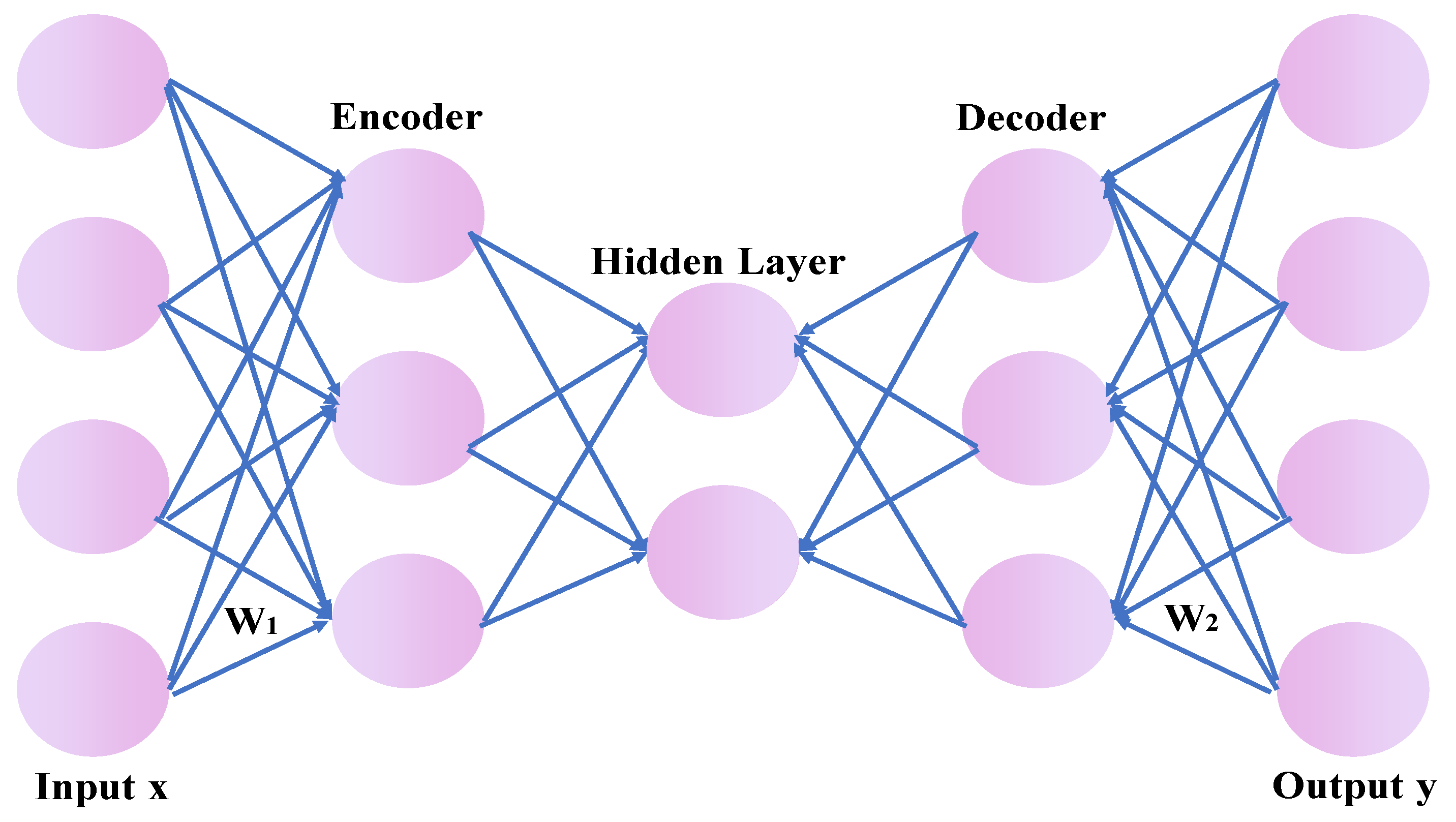
Since the restoration task corresponding to this article is mainly the first task type, it is considered to have good meaning to be able to restore the characteristics of the original data through the learned elements in the data recovery scheme. Currently, the usual method of this type is mainly the Autoencoder, and the architecture of Autoencoder is as follows:
It can be seen from Figure 1 that the Autoencoder mainly includes an encoder and a decoder [31], and its structure is usually symmetrical. Overall, the purpose of the Autoencoder is to reconstruct the input data in the output layer. The ideal situation is that the output signal, y, is the same as the input signal, x. Thus, the encoding and decoding process of Autoencoder can be described as the following expressions:
where Equation (2) denotes the encoding process, Equation (3) is the decoding process, and and represent the weight and bias of the encoder, respectively. Similarly, and are the weight and bias of the decoder, respectively. represents the non-linear transformation in the encoding process, with the more commonly used ones being sigmoid, tanh, and Relu, and denotes the nonlinear transformation or affine transformation in the decoding process. Consequently, the loss function of the Autoencoder is to minimize the error between y and x, which is expressed as follows:
In Equation (4), W represents weight and b denotes bias. In addition, L is the loss function calculated by mean square error.
2.2. Proposed Network Architecture
Atmospheric turbulence distortion of an image is a complex physical process. It produces geometric distortion, space and time-variant defocus blur, and motion blur. According to the literature (Zhu and Milanfar) [32], the imaging process can be formulated as follows:
where x denotes the ideal image, the “∗” is namely convolution operation, and and represent the geometric deformation matrix and blurring matrix, respectively. denotes additive noise and is the j-th observed frame. When we ignore the impact of noise, the formula above can be simplified to:
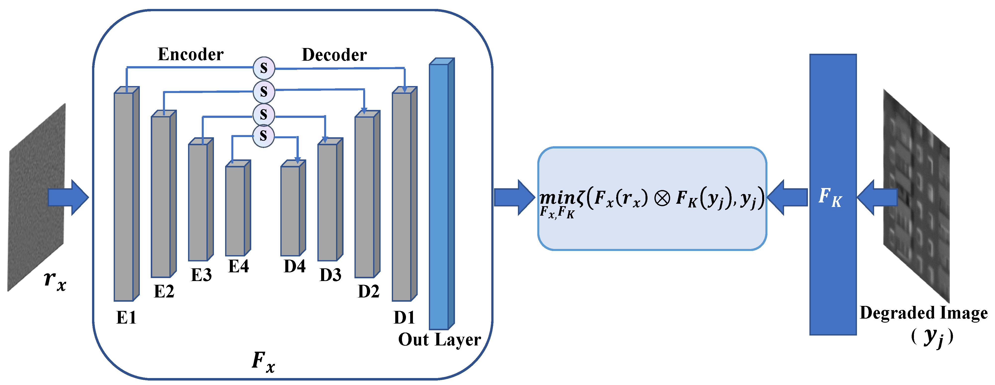
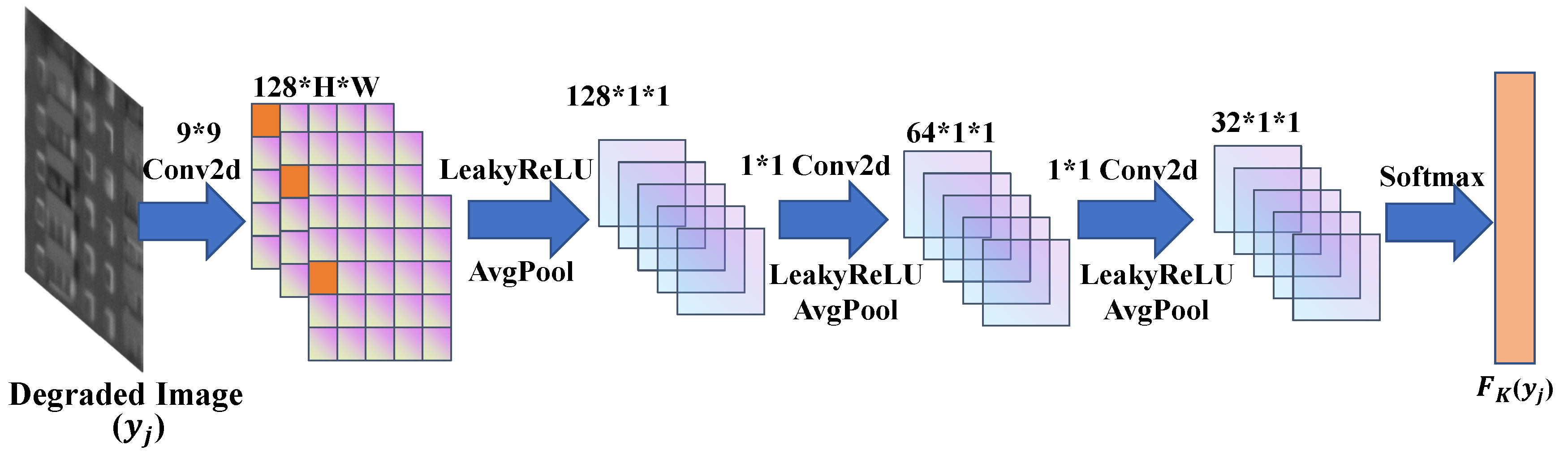
where denotes the turbulence-distorted operator. In that case, the proposed framework is shown in Figure 2. Specifically, it contains two parts: and . The function of is mainly to generate the latent clear image when inputting two-dimensional random noise (). is composed of a four-layer symmetrical encoder–decoder network, and each layer of encoding and decoding modules is linked by the skip connection, which can effectively reduce the problems of gradient disappearance and network degradation. Simultaneously, the function of is to generate a turbulence-distorted operator by inputting a real degraded image (), which is mainly a fully convolutional network (seen in Figure 3) that can restore the complicated 2D degraded kernel. Moreover, each layer of network parameters of are shown in Figure 4. In most cases, the turbulence-degraded image can be equivalent to the convolution generation of the turbulence-degraded operator and the potentially clear image [32,33]. Therefore, by substituting x and with and , the deconvolution can be written as follows:
where and represent the i-th and m-th elements, respectively.
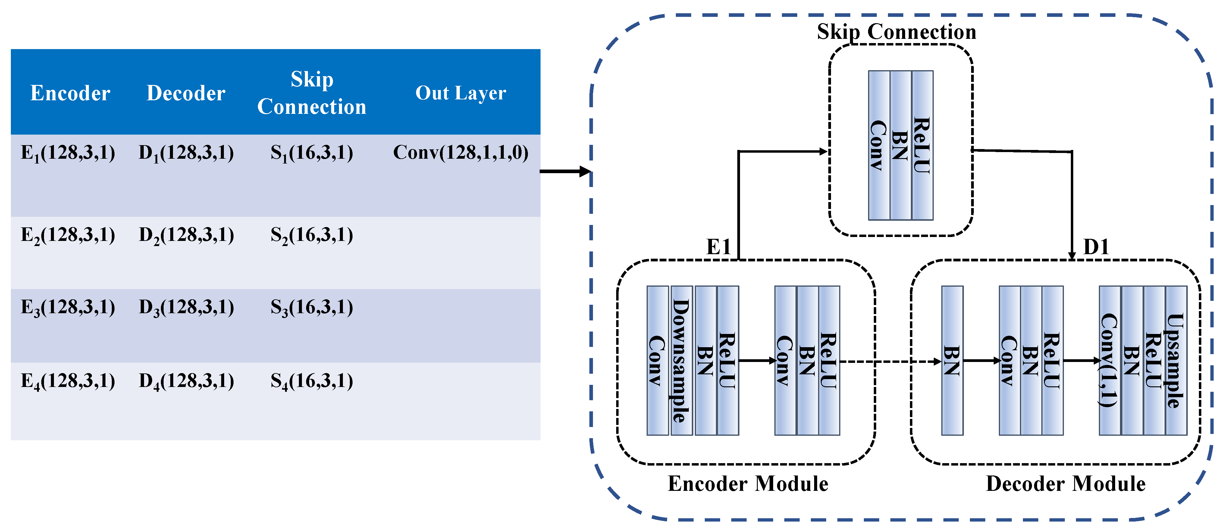
Figure 4 shows the specific composition of the network. The network used the same encoder–decoder architecture. Therefore, the network composition for one layer of the encoder–decoder is listed, which is roughly similar to the composition of the DIP network [16]. The down-sampling is implemented using stride = 2, and the up-sampling is implemented by using 2× bilinear interpolation.
2.3. Regularization by Denoising (RED)
In essence, the image restoration process is a classical ill-posed problem, especially for the unconstrained self-supervised learning solution used in this research. Therefore, we added a denoising regular term after the existing objective function to produce a better restored image. The denoising regularization term was first proposed by Romano et al. [34]. It uses existing denoisers to regularize the inverse problem and relies on the Alternating Direction Multiplier Method (ADMM) optimization technology. Meanwhile, it has been proven effective in image denoising, over-segmentation, deblurring, etc. The objective function after adding denoising regularization is:
Equation (9) is the objective function used in this study, where represents denoising regularization. Here, ADMM and the Augmented Lagrangian penalty term are introduced. The specific expression is shown in the following formula:
where u is a set of Lagrangian multiplier vectors of equality constraints. The ADMM algorithm mainly updates the above three parameters: u, x, and , and when fixing x and u, is updated by solving the following expression:
When fixing and u, x is updated by solving the following form:
According to the Augmented Lagrangian (AL) method [35], the update of parameter u can be realized by following Equation (13).
2.4. Implementation Details
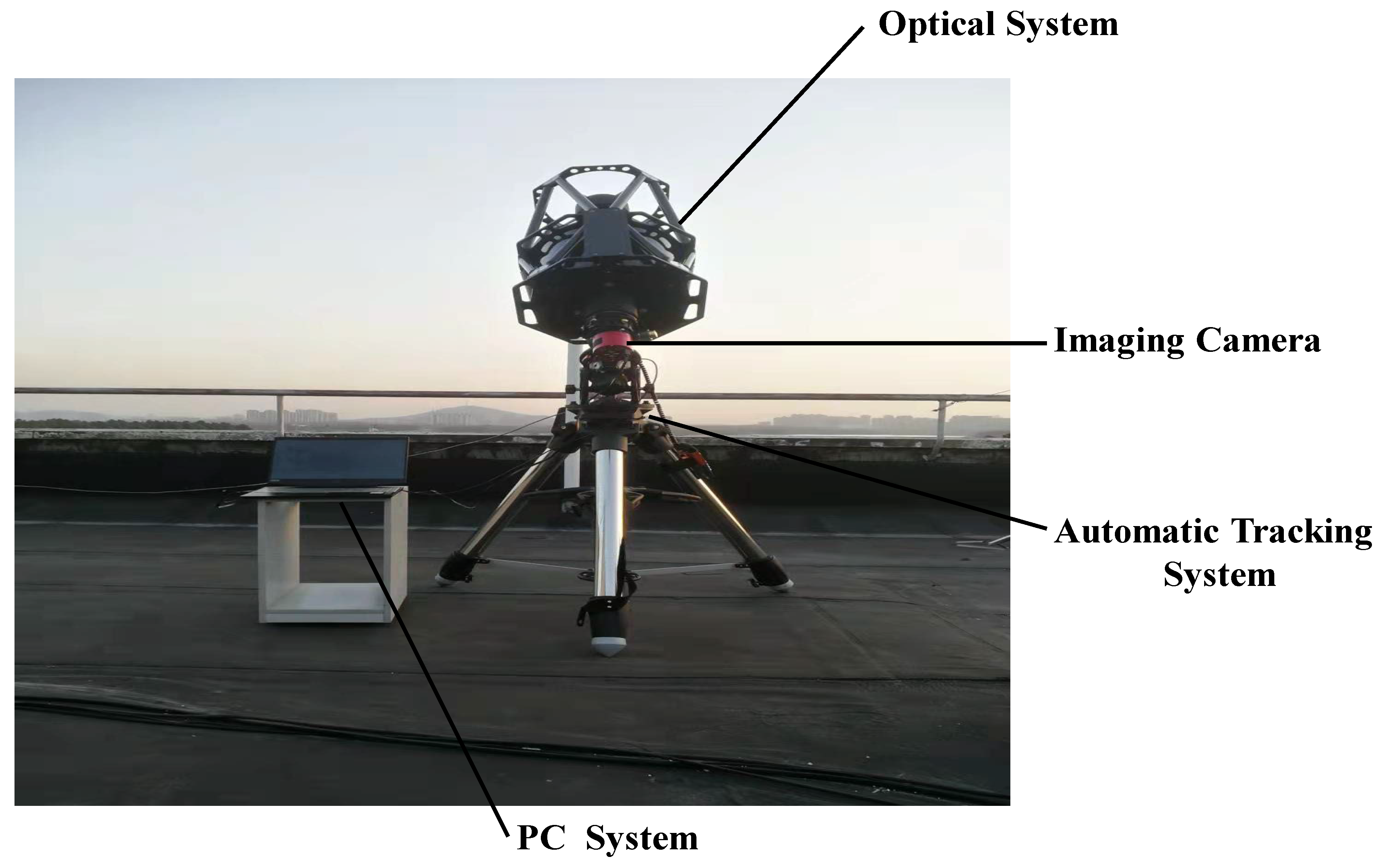
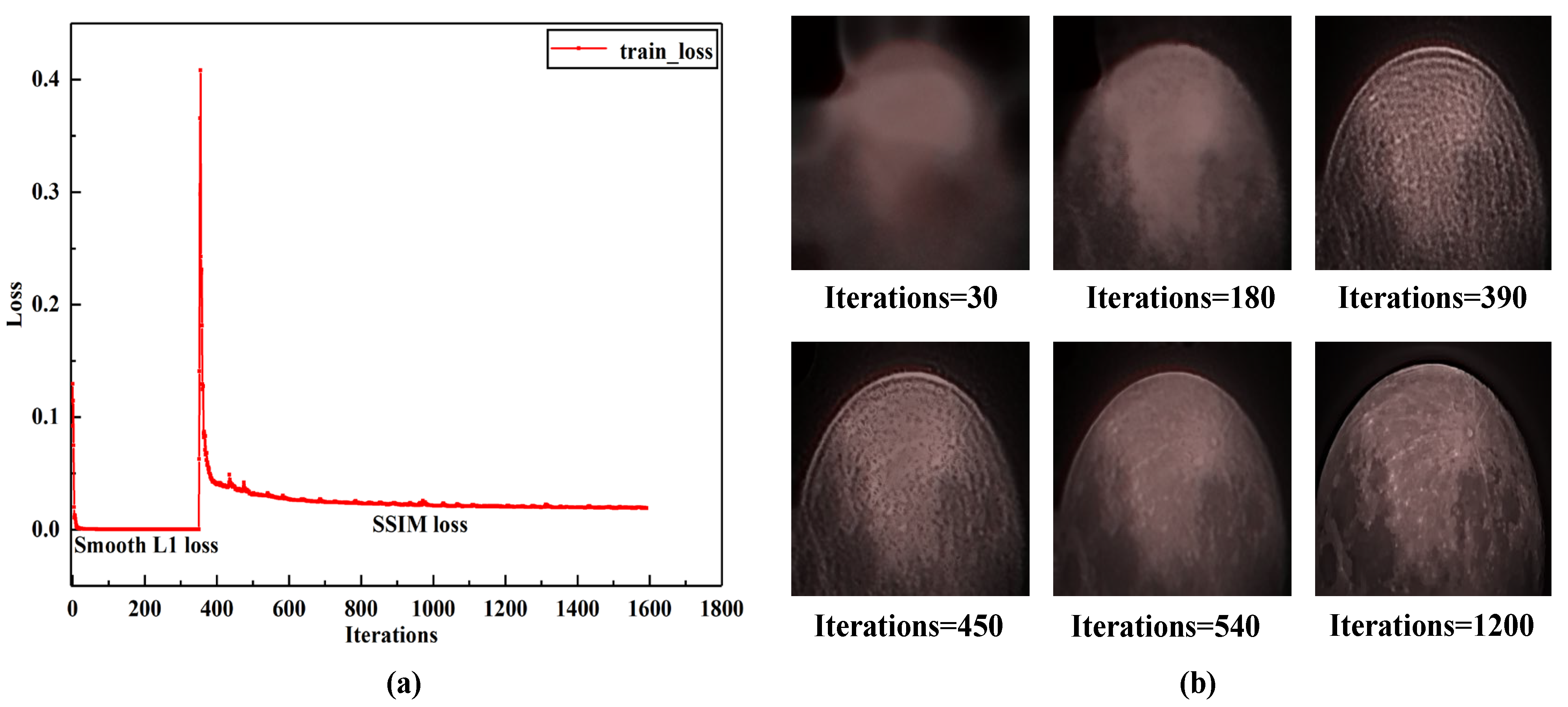
The designed network is implemented in the PyTorch1.5 deep learning framework [36] and is trained on the ubuntu 18.04 system using a single NVIDIA GTX 1080Ti GPU. As shown in Figure 2, the input of the network is a two-dimensional random noise, and is sampled from the uniform distribution. On the other hand, the input of the network is a single distorted image frame. Furthermore, the network does not also rely on external data for the pre-training and only uses the designed objective function for continuous iterative calculation. Since the model weight is randomly initialized, choosing a larger learning rate will cause the model to oscillate; the initial learning rate is set to 0.001. Meanwhile, the loss function is set at two-stage loss to ensure a superior output restoration effect. The first stage loss function is set to smooth L1 loss [37], and using the pixel-by-pixel comparison, the contour of the image to be restored can be quickly obtained. When the iteration reaches a certain number of times, the loss function does not decrease anymore, and the SSIM loss is used as the second stage loss function to restore the image detail information [38]. Our observation system (Figure 5), listed in Table 1, mainly includes a Richey–Chretien telescope (RC12), a German equatorial telescope mount (CGX-L), an optical camera (ASI071MC Pro), and a high-performance computer (PC). Subsequently, the iterative process of the turbulence-distorted moon image taken by our system is shown in Figure 6a, and the output result of each stage in Figure 6b.
3. Comparative Experiment Preparation
3.1. Existing Restoration Methods
The proposed method is compared with the following state-of-the-art methods, including physics-based approaches (CLEAR [39], SGL [40], IBD [41]), and a learning-based method (DNCNN [42]). Specifically, the CLEAR algorithm uses a region-level fusion algorithm based on a binary tree-based wavelet transform to solve the turbulence distorted problem. A Sobolev Gradient method was applied by the SGL algorithm to sharpen individual frames and mitigate the temporal distortions with the Laplace operator [43]. The IBD algorithm directly estimates the blur kernel of the degraded image and latent clear image according to prior conditions. DNCNN is based on supervised learning [42], which was proven to play an important role in restoring turbulence-distorted images by researchers from the University of Bristol [44]. The outputs of all compared methods are generated using the authors’ codes, with the related parameters unchanged.
Obviously, DNCNN can be used to recover high-quality images when it is trained on a large synthetic turbulence dataset. Therefore, we use the power spectrum inversion method combined with sub-harmonics to simulate turbulence-degraded images of different intensities as the training set. The random phase screen of atmospheric turbulence is obtained by using Fourier transform, and the equation can be expressed as follows [45]:
where and are the spatial frequencies in the m and z directions, respectively. is a complex Gaussian random number. Therefore, this power spectral density function can be written as follows:
represents the atmospheric coherence length, which is a characteristic scale reflecting the intensity of the atmospheric turbulence. According to the parameter settings in Table 2, the random phase screens with different turbulence intensities are finally obtained.
Original images are from the Hubble official website (URL: https://esahubble.org/images/ (accessed on 27 July 2023)), and examples of simulated degraded images are as follows (D/r0 represents different turbulence intensity).
As shown in Figure 7, the Point Spread Function (PSF), the phase screen, and the simulated turbulence-degraded images obtained with different intensities are denoted, respectively. There are 1800 images, including training data (1500) and validation data (300), and all image sizes are 256 × 256. We use the training set to pre-train the DNCNN network. The hyperparameter settings of the network adopt the default settings in the original paper. When the number of iterations reaches approximately 150 epochs, the loss function curve has stabilized and no longer continues to converge downwards; the DNCNN model reaches the minimum convergence standard at this time.
3.2. Experimental Datasets
It is necessary to obtain real degraded images under different conditions for experimental analysis to test the proposed networks’ robustness and adaptability. Therefore, extensive experiments with the proposed algorithm and four comparison methods are conducted in Hirsch’s dataset [46], the Open Turbulent Image Set (OTIS) [47], and the YouTube dataset, respectively. These datasets are introduced as follows:
Hirsch’s dataset: Hirsch’s dataset was used for testing the Efficient Filter Flow (EFF) framework. The dataset was taken by using the Canon EOS 5D Mark Ⅱ camera, equipped with a 200 mm zoom lens. By capturing a static scene of the hot air discharged from the vents of the building, the image sequence is a video stream of 100 frames (the exposure time of each frame is 1/250 s) degraded due to spatial changes and blurring. The image sequences mainly include chimneys, buildings, water tanks, etc.
OTIS: OTIS was put forward by Jérôme Gilles et al. to make the comparison between algorithms. All image sequences are real turbulence-distorted images acquired in the hot summer. The dataset includes 4628 static sequences and 567 dynamic sequences. The turbulence impact is also divided into three levels: strong, medium, and weak. All sequences are captured with GoPro Hero 4 Black cameras, and the camera equipment is modified with a Ribcage Air chassis permitting to adapt to different lens types.
YouTube dataset: Since there is no publicly available astronomical object turbulence distorted image dataset, we obtained astronomical object videos from YouTube. These video frames include the moon’s surface and Jupiter taken by foreign astronomy enthusiasts. This data captured comes from different devices, which will put more tests on the restoration effect for the proposed algorithm.
3.3. Evaluation Metrics
This study is aimed at the restoration of real turbulence distorted images. Therefore, no-reference metrics are used for objective evaluation. The selected no-reference metrics include: Entropy, Average Gradient, Natural Image Quality Evaluator (NIQE) [48], and Blind/Referenceless Image Spatial Quality Evaluator (BRISQUE) [49]. Simultaneously, the specific explanations are as follows:
Entropy:
Typically, it indicates the average amount of information contained in the image. In particular, the greater the information entropy of an image, the better the image quality. The definition of which is as follows:
where p() is the probability that a random event x is .
Average Gradient:
Average Gradient puts more emphasis on the layering of the image and whether the image details are rich, which is expressed as follows:
where m and n represent the width and height of the image, respectively, and i and j denotes the position of the image pixel. Generally, the larger the Average Gradient value, the more the detailed the image, and the clearer the image.
4. Results and Discussion
4.1. Near-Ground Turbulence-Distorted Image Results
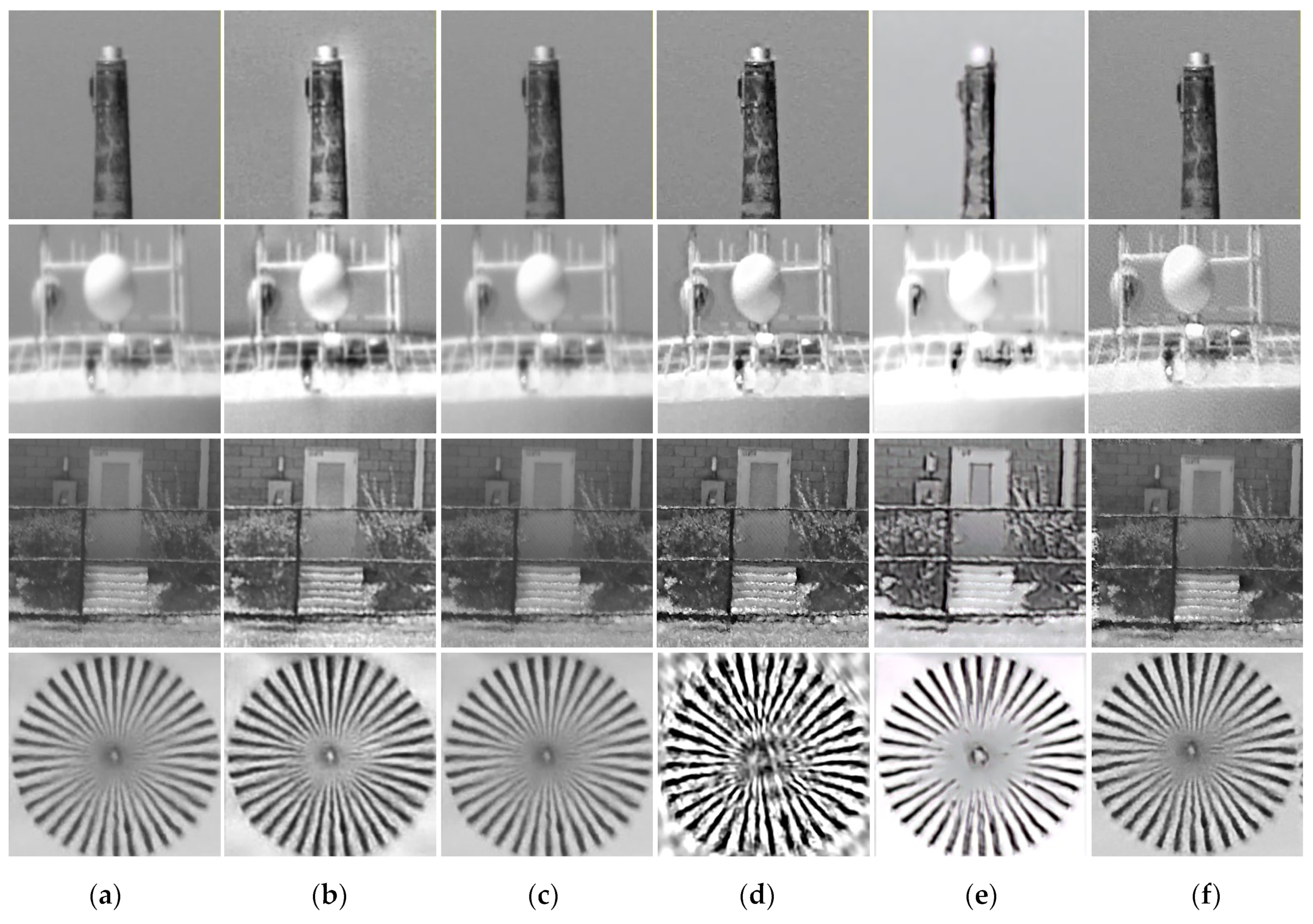
The real near-ground turbulence-distorted image contains two parts, which are randomly selected from Hirsch’s dataset [46] and OTIS [47]. As shown in Figure 8, the first two rows of degraded images are from Hirsch’s dataset, and the last two rows are from the OTIS. (b), (c), (d), and (e) are the restored results by the abovementioned algorithms, and (f) is the network proposed output. Meanwhile, we use no-reference evaluation metrics to evaluate the effect of image restoration. Table 3 presents the average values of the results by several algorithms. Entropy estimates the complexity of the image texture; the Average Gradient refers to the obvious difference in grayscale near the border of the image or on both sides of the shadow line, and reflects the rate of density change in the multi-dimensional direction of the image to characterize the relative clarity; NIQE is based on the construction of a ‘quality aware’ collection of statistical features based on a simple and successful space domain Natural Scene Statistic (NSS) model, and these features are derived from a corpus of natural, undistorted images [48]; BRISQUE does not compute distortion-specific features, such as ringing, blur, or blocking, but instead uses scene statistics of locally normalized luminance coefficients to quantify possible losses of “naturalness” in the image due to the presence of distortions, thereby leading to a holistic measure of quality [49]. The specific content is shown in Figure 8 and Table 3.
For the above recovery results, it can seem that different degrees of artifacts will appear for all restoration results. Significantly, the output result of the IBD algorithm may appear as deformation (see the last row in Figure 8d), and the CLEAR and DNCNN algorithms will change the background of the testing images. Additionally, it can be clearly found that the various image quality indicators of the DNCNN algorithm are worse than the indicators of the inputting degraded image. The results have been marked blue, which illustrates that the DNCNN pre-trained with simulated data may aggravate inputting image degradation. Related reasons will be analyzed in subsequent ablation experiments. Regardless of Hirsch’s dataset or OTIS, the proposed approach has shown an excellent restoration effect, especially using the BRISQUE indicator evaluation.
4.2. Turbulence-Degraded Astronomical Object Results
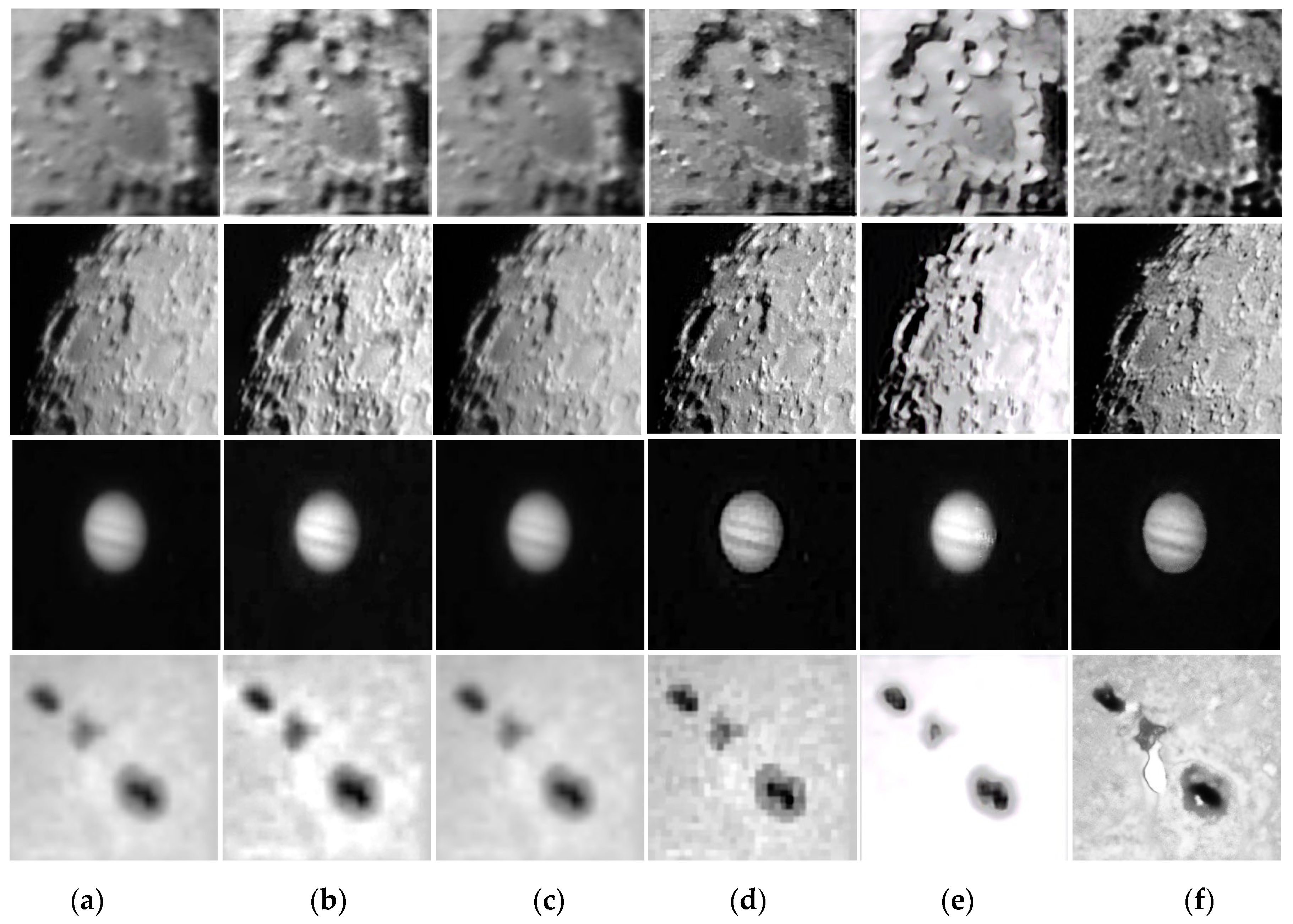
In this section, test images include the surface of the moon and Jupiter from YouTube. Moreover, we add a sunspot image taken by the National Astronomical Observatory in order to enrich the content of the test data. Accordingly, the abovementioned images restoration effects and no-reference metrics are shown in the following figure.
The comprehensive experimental results of different algorithms are shown in Figure 9 and Table 4. Specifically, the SGL algorithm has almost no improvement on the input degraded image, which may be because the default input of the SGL is video sequences. The restoration effect is ineffective for a single turbulence distorted image since it lacks more feature information. The IBD algorithm seems to have a good restoration effect from a subjective point of view. Still, the objective evaluation index did not produce such a result, which may be due to the IBD algorithm having enhanced the restoration image. The DNCNN algorithm changes the main characteristics of the image, which is especially obvious in the last row in Figure 9e. Instead, the proposed model fully combines the advantages of regularization and machine learning, so it achieves a relatively excellent restoration effect.
4.3. Motion-Blurred Image Results
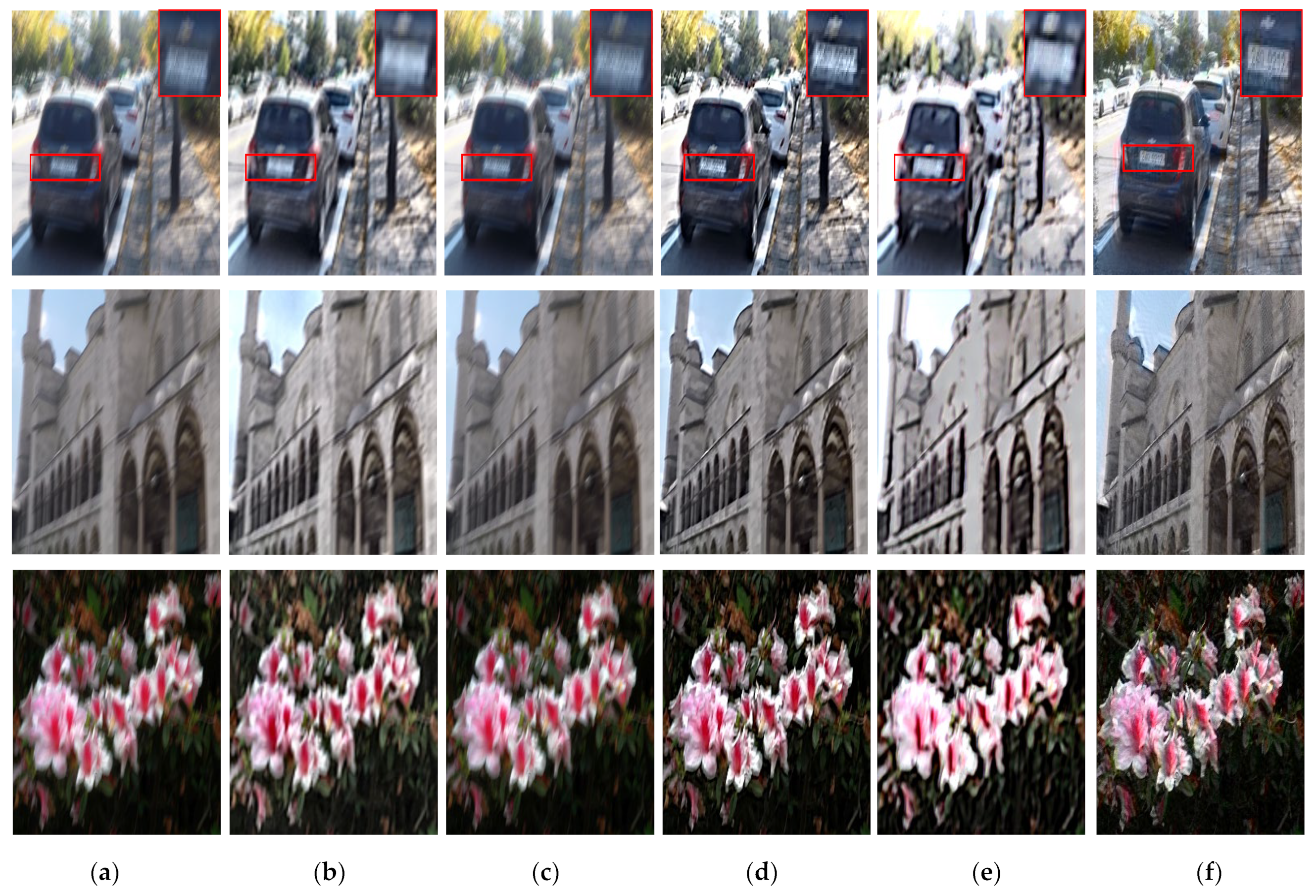
As stated in the first half of the article, the approach proposed can output excellent results without pre-training. Therefore, the proposed model is still applicable for a single motion-blurred image. To verify the restoration effect on motion-blurred images, we randomly choose motion-blurred images from the GoPro dataset and the Internet to verify our idea [50]. The specific restoration effect and objective evaluation are displayed in Figure 10 and Table 5:
The above comprehensive experimental results show that: (1) in the car scene, the restoration results of the four comparative algorithms cannot effectively see the license plate information and the vehicle brand, and there are varying degrees of artifacts; (2) the output results of the CLEAR algorithm seem to increase the blur effect of the image, which may be because the physical model of the CLEAR algorithm does not match with the motion blur; (3) the supervised learning (DNCNN) has poor generalization ability for motion-blurred images (blue marker); and (4) from the comprehensive analysis of the visual effects of multiple indicators and restored images, the proposed approach is the best of all comparison methods.
4.4. Ablation Study
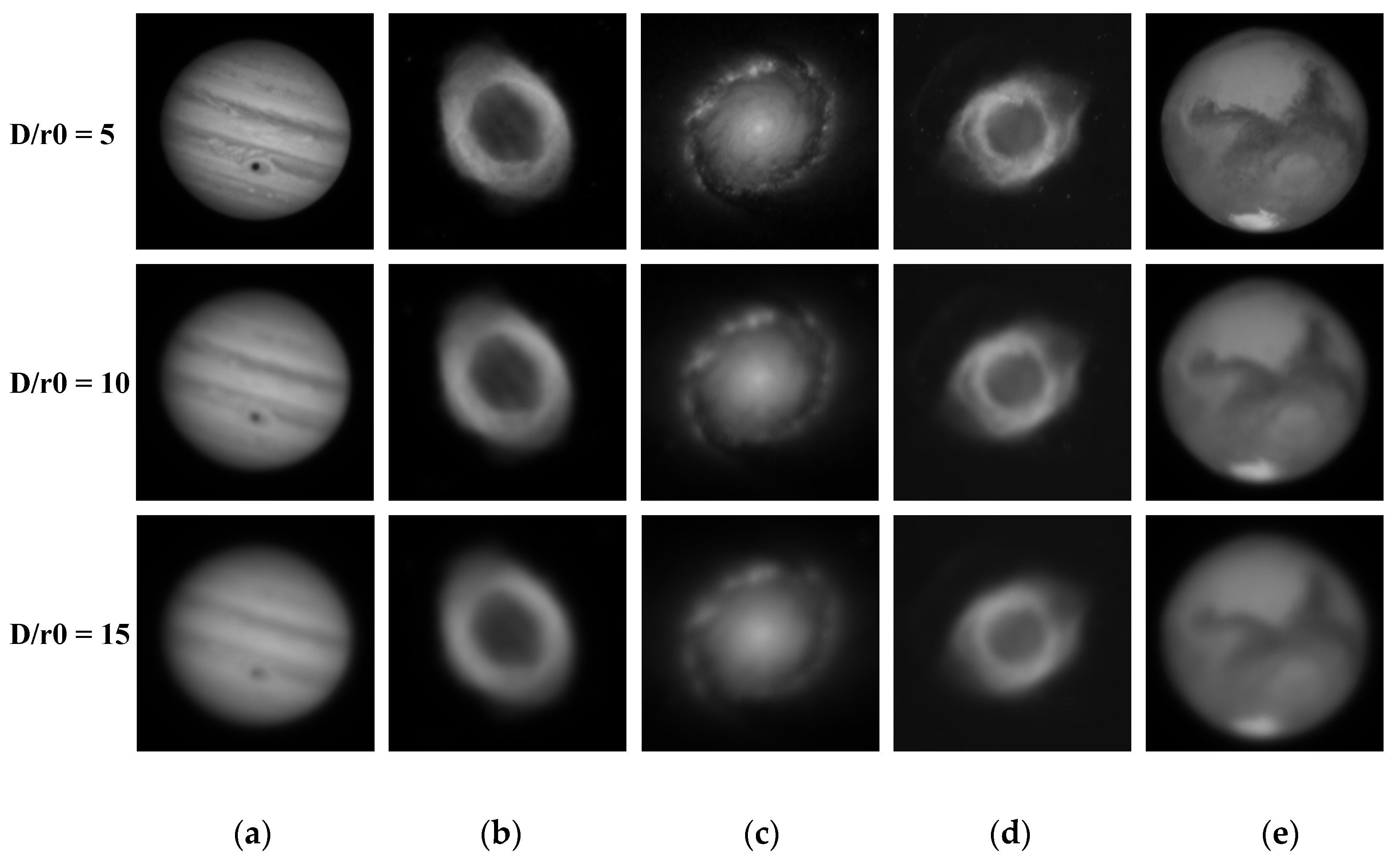
As previously mentioned, it is not difficult to see that the self-supervised model proposed has a better restoration effect on the real degraded images than the DNCNN network by analyzing the above experiments (Table 3, Table 4 and Table 5). The reason may be that the pre-trained simulated data is inconsistent with the data in the natural state. Therefore, ablation experiments are conducted to prove whether the analysis is true. There are 150 turbulence-degraded images randomly selected from the untrained simulation data, including 50 appearances with D/r0 = 5, D/r0 = 10, and D/r0 = 15, respectively. Examples of testing images are illustrated in Figure 11; there are the Jupiter image, the Nebula1 image, the Galaxy image, the Nebula2 image, and the Mars image:
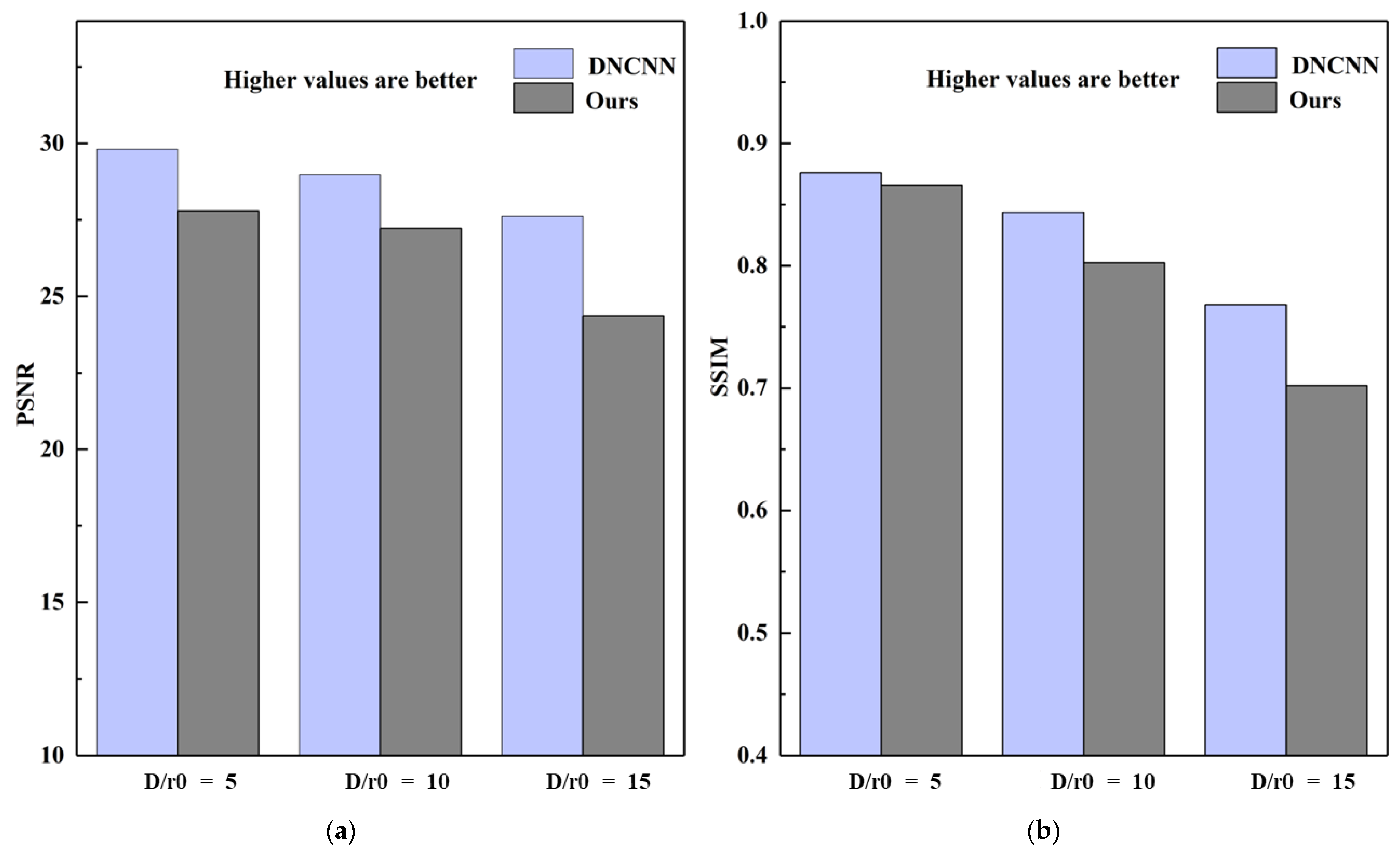
The simulated degraded images of different intensities are sent to DNCNN and the proposed network for testing. The test indicators are the Peak Signal to Noise Ratio (PSNR) and Structural Similarity (SSIM). The specific diagrams are as follows.
Figure 12 shows that when the image input is consistent with the training dataset, the turbulence intensity is relatively weak (D/r0 = 5), or when the turbulence intensities are medium and strong (D/r0 = 10, D/r0 = 15), the DNCNN network achieves better results than the proposed algorithm. Therefore, it can be explained that when the data distribution of the pre-trained set and the test set are consistent, the output result of DNCNN is better. When the data distribution is inconsistent, the restoration results by DNCNN are shown in Table 3, Table 4 and Table 5. The output is often not as expected, and the network even aggravates the degradation of the inputting. Therefore, the ablation experiment demonstrates that the DNCNN architectures have trouble with generalization outside of the training data (as do most supervised neural networks). Instead, the proposed approach (ours) does not need to rely on external data to drive, and it may be more adaptable and robust to real degraded images.
5. Conclusions
A large sample size of training data is typically necessary for solving tasks using deep learning approaches, but unfortunately, there is limited turbulence-distorted data available. In this study, firstly, we presented a blind restoration method for a single turbulence distorted image based on self-supervised learning. The designed framework is mainly aimed at real turbulence-degraded images without labels. To our knowledge, this work is also the first to apply self-supervised learning to the task of alleviating the turbulence effect on images. Subsequently, we also curate a natural turbulent dataset from Hirsch’s dataset, OTIS, and YouTube to show the generalist ability of the proposed model. Moreover, we conducted ablation experiments to further verify the differences between supervised learning and the proposed self-supervised learning method. Eventually, through the above work carried out, we can draw the following conclusions.
The proposed model can recover the information of the image itself well under different levels. Additionally, instead of using a single loss function, this approach proposed uses the first stage of smooth L1 loss, and the second stage SSIM loss function is employed so that the overall contour of the image can be restored firstly, and then the edges and details can be recovered. Meanwhile, the brightness of the image does not change during this processing. For the most critical part of the network, an effective self-supervised learning mechanism is designed to fully extract the turbulence-distorted features implicit in the image itself, which depends on repeated experiments and parameterized debugging. In particular, quantitative evaluation of four image quality indicators shows that the proposed method has a more superior performance than the competing methods, both in terms of sharpness and visual consistency. Furthermore, unlike previous methods, our approach neither uses any prior knowledge about atmospheric turbulence conditions nor requires the fusion of multiple images to get a single restored result, which has great engineering value in long-range video surveillance, defense systems, and drone imaging systems. However, the proposed algorithm still needs some improvements. For instance, there will be artifacts in some restored results (see the Figure 8(f2) (the f2 refers to the second image in column f) and Figure 9(f1) (the f1 means the first image in column f)), which will be optimized with the following debugging.
In the future, we also intend to remove turbulence on video and consider combining some atmospheric turbulence parameters (e.g., , ) measured by our instruments to the neural network model for mitigating the turbulence effect. Furthermore, since the network needs multiple iterations in the process of outputting results, it is not suitable for astronomical observation and video surveillance in the real state. We hope the proposed model can be embedded in high-level vision tasks and considered a “real-time” task in the following work. Meanwhile, in the following remote sensing observations, the parameters of the proposed self-supervised learning network are optimized by acquiring a large number of real turbulence-degradation images.
Author Contributions
Conceptualization, Y.G. and X.W.; software, Y.G.; validation, formal analysis, Y.G. and C.Q.; data curation, Q.Y. and L.L.; instrument, S.S.; writing—original draft preparation, Y.G.; writing—review and editing, X.Q.; visualization, Q.Y.; supervision, X.H.; project administration and funding acquisition, X.W. All authors have read and agreed to the published version of the manuscript.
Funding
This research was funded by the National Natural Science Foundation of China (Grant No. 91752103), the Foundation of Advanced Laser Technology Laboratory of Anhui Province (Grant No. AHL2021QN02), the National Natural Science Foundation of China (Grant No. 42027804), and the Foundation of Key Laboratory of Science and Technology Innovation of Chinese Academy of Sciences (Grant No. CXJJ-21S028).
Data Availability Statement
The data were prepared and analyzed in this study.
Acknowledgments
We thank all anonymous reviewers for their comments and suggestions. In addition, the authors would like to thank Xiaoqing Wu and Chun Qing for their patience, help, and guidance.
Conflicts of Interest
The authors declare no conflict of interest.
References
- Chen, E.; Haik, O.; Yitzhaky, Y. Detecting and tracking moving objects in long-distance imaging through turbulent medium. Appl. Opt. 2014, 53, 1181–1190. [Google Scholar] [CrossRef] [PubMed]
- Chen, E.; Haik, O.; Yitzhaky, Y. Online spatio-temporal action detection in long-distance imaging affected by the atmosphere. IEEE Access 2021, 9, 24531–24545. [Google Scholar] [CrossRef]
- Roggemann, M.C.; Welsh, B.M.; Hunt, B.R. Imaging Through Turbulence; CRC Press: Boca Raton, FL, USA, 1996. [Google Scholar]
- Labeyrie, A. Attainment of diffraction limited resolution in large telescopes by Fourier analysing speckle patterns in star images. Astron. Astrophys. 1970, 6, 85–87. [Google Scholar]
- Ayers, G.; Dainty, J.C. Iterative blind deconvolution method and its applications. Opt. Lett. 1988, 13, 547–549. [Google Scholar] [CrossRef]
- Fried, D.L. Probability of getting a lucky short-exposure image through turbulence. JOSA 1978, 68, 1651–1658. [Google Scholar] [CrossRef]
- Carasso, A.S. APEX blind deconvolution of color Hubble space telescope imagery and other astronomical data. Opt. Eng. 2006, 45, 107004. [Google Scholar] [CrossRef]
- Radenović, F.; Tolias, G.; Chum, O. CNN image retrieval learns from BoW: Unsupervised fine-tuning with hard examples. In Proceedings of the European Conference on Computer Vision, Amsterdam, The Netherlands, 11–14 October 2016; pp. 3–20. [Google Scholar]
- Liu, P.; Zhang, H.; Zhang, K.; Lin, L.; Zuo, W. Multi-level wavelet-CNN for image restoration. In Proceedings of the IEEE Conference on Computer Vision and Pattern Recognition Workshops, Salt Lake City, UT, USA, 18–22 June 2018; pp. 773–782. [Google Scholar]
- Boulila, W.; Sellami, M.; Driss, M.; Al-Sarem, M.; Safaei, M.; Ghaleb, F.A. RS-DCNN: A novel distributed convolutional-neural-networks based-approach for big remote-sensing image classification. Comput. Electron. Agric. 2021, 182, 106014. [Google Scholar] [CrossRef]
- Quan, Y.; Chen, Y.; Shao, Y.; Teng, H.; Xu, Y.; Ji, H. Image denoising using complex-valued deep CNN. Pattern Recogn. 2021, 111, 107639. [Google Scholar] [CrossRef]
- Gao, Z.; Shen, C.; Xie, C. Stacked convolutional auto-encoders for single space target image blind deconvolution. Neurocomputing 2018, 313, 295–305. [Google Scholar] [CrossRef]
- Chen, G.; Gao, Z.; Wang, Q.; Luo, Q. Blind de-convolution of images degraded by atmospheric turbulence. Appl. Soft Comput. 2020, 89, 106131. [Google Scholar] [CrossRef]
- Chen, G.; Gao, Z.; Wang, Q.; Luo, Q. U-net like deep autoencoders for deblurring atmospheric turbulence. J. Electron. Imaging 2019, 28, 053024. [Google Scholar] [CrossRef]
- Bai, X.; Liu, M.; He, C.; Dong, L.; Zhao, Y.; Liu, X. Restoration of turbulence-degraded images based on deep convolutional network. In Proceedings of the Applications of Machine Learning, Boca Raton, FL, USA, 16–19 December 2019; p. 111390B. [Google Scholar]
- Ulyanov, D.; Vedaldi, A.; Lempitsky, V. Deep image prior. In Proceedings of the Proceedings of the IEEE Conference on Computer Vision and Pattern Recognition, Salt Lake City, UT, USA, 18–22 June 2018; pp. 9446–9454. [Google Scholar]
- Chen, B.; Rouditchenko, A.; Duarte, K.; Kuehne, H.; Thomas, S.; Boggust, A.; Panda, R.; Kingsbury, B.; Feris, R.; Harwath, D. Multimodal clustering networks for self-supervised learning from unlabeled videos. In Proceedings of the IEEE/CVF International Conference on Computer Vision, Montreal, BC, Canada, 11–17 October 2021; pp. 8012–8021. [Google Scholar]
- Yaman, B.; Hosseini, S.A.H.; Akcakaya, M. Zero-Shot Self-Supervised Learning for MRI Reconstruction. In Proceedings of the International Conference on Learning Representations, Vienna, Austria, 3–7 May 2021. [Google Scholar]
- Mahapatra, D.; Ge, Z.; Reyes, M. Self-supervised generalized zero shot learning for medical image classification using novel interpretable saliency maps. IEEE Trans. Med. Imaging 2022, 41, 2443–2456. [Google Scholar] [CrossRef] [PubMed]
- Kolesnikov, A.; Zhai, X.; Beyer, L. Revisiting Self-Supervised visual representation learning. In Proceedings of the IEEE/CVF Conference on Computer Vision and Pattern Recognition, Long Beach, CA, USA, 15–20 June 2019; pp. 1920–1929. [Google Scholar]
- Zhai, X.; Oliver, A.; Kolesnikov, A.; Beyer, L. S4l: Self-supervised semi-supervised learning. In Proceedings of the IEEE/CVF International Conference on Computer Vision, Seoul, Republic of Korea, 27 October–2 November 2019; pp. 1476–1485. [Google Scholar]
- Lee, H.; Hwang, S.J.; Shin, J. Self-supervised label augmentation via input transformations. In Proceedings of the International Conference on Machine Learning, Online, 13–18 July 2020; pp. 5714–5724. [Google Scholar]
- Liu, X.; Zhang, F.; Hou, Z.; Mian, L.; Wang, Z.; Zhang, J.; Tang, J. Self-supervised learning: Generative or contrastive. IEEE Trans. Knowl. Data Eng. 2021, 35, 857–876. [Google Scholar] [CrossRef]
- Hua, T.; Wang, W.; Xue, Z.; Ren, S.; Wang, Y.; Zhao, H. On feature decorrelation in self-supervised learning. In Proceedings of the IEEE/CVF International Conference on Computer Vision, Montreal, BC, Canada, 11–17 October 2021; pp. 9598–9608. [Google Scholar]
- Wu, J.; Zhang, T.; Zha, Z.-J.; Luo, J.; Zhang, Y.; Wu, F. Self-supervised domain-aware generative network for generalized zero-shot learning. In Proceedings of the IEEE/CVF Conference on Computer Vision and Pattern Recognition, Seattle, WA, USA, 13–19 June 2020; pp. 12767–12776. [Google Scholar]
- Eckart, B.; Yuan, W.; Liu, C.; Kautz, J. Self-supervised learning on 3d point clouds by learning discrete generative models. In Proceedings of the IEEE/CVF Conference on Computer Vision and Pattern Recognition, Nashville, TN, USA, 20–25 June 2021; pp. 8248–8257. [Google Scholar]
- Sermanet, P.; Lynch, C.; Chebotar, Y.; Hsu, J.; Jang, E.; Schaal, S.; Levine, S.; Brain, G. Time-contrastive networks: Self-supervised learning from video. In Proceedings of the 2018 IEEE International Conference on Robotics and Automation (ICRA), Brisbane, Australia, 21–25 June 2018; pp. 1134–1141. [Google Scholar]
- Wang, X.; Zhang, R.; Shen, C.; Kong, T.; Li, L. Dense contrastive learning for self-supervised visual pre-training. In Proceedings of the IEEE/CVF Conference on Computer Vision and Pattern Recognition, Nashville, TN, USA, 20–25 June 2021; pp. 3024–3033. [Google Scholar]
- Donahue, J.; Krähenbühl, P.; Darrell, T. Adversarial feature learning. arXiv 2016, arXiv:1605.09782. [Google Scholar]
- Dumoulin, V.; Belghazi, I.; Poole, B.; Mastropietro, O.; Lamb, A.; Arjovsky, M.; Courville, A. Adversarially learned inference. arXiv 2016, arXiv:1606.00704. [Google Scholar]
- Ballard, D.H. Modular learning in neural networks. In Proceedings of the Aaai, Seattle, WA, USA, 13–17 July 1987; pp. 279–284. [Google Scholar]
- Zhu, X.; Milanfar, P. Removing atmospheric turbulence via space-invariant deconvolution. IEEE Trans. Pattern Anal. Mach. Intell. 2012, 35, 157–170. [Google Scholar] [CrossRef]
- Furhad, M.H.; Tahtali, M.; Lambert, A. Restoring atmospheric-turbulence-degraded images. Appl. Opt. 2016, 55, 5082–5090. [Google Scholar] [CrossRef]
- Romano, Y.; Elad, M.; Milanfar, P. The little engine that could: Regularization by denoising (RED). SIAM J. Imag. Sci. 2017, 10, 1804–1844. [Google Scholar] [CrossRef]
- Afonso, M.V.; Bioucas-Dias, J.M.; Figueiredo, M.A. Fast image recovery using variable splitting and constrained optimization. IEEE Trans. Image Process. 2010, 19, 2345–2356. [Google Scholar] [CrossRef]
- Paszke, A.; Gross, S.; Chintala, S.; Chanan, G.; Yang, E.; DeVito, Z.; Lin, Z.; Desmaison, A.; Antiga, L.; Lerer, A. Automatic differentiation in pytorch. In Proceedings of the Conference and Workshop on Neural Information Processing Systems, Long Beach, CA, USA, 4–9 December 2017; pp. 1–4. [Google Scholar]
- Girshick, R. Fast r-cnn. In Proceedings of the IEEE International Conference on Computer Vision, Santiago, Chile, 7–13 December 2015; pp. 1440–1448. [Google Scholar]
- Wang, Z.; Bovik, A.C.; Sheikh, H.R.; Simoncelli, E.P. Image quality assessment: From error visibility to structural similarity. IEEE Trans. Image Process. 2004, 13, 600–612. [Google Scholar] [CrossRef]
- Anantrasirichai, N.; Achim, A.; Kingsbury, N.G.; Bull, D.R. Atmospheric turbulence mitigation using complex wavelet-based fusion. IEEE Trans. Image Process. 2013, 22, 2398–2408. [Google Scholar] [CrossRef] [PubMed]
- Lou, Y.; Kang, S.H.; Soatto, S.; Bertozzi, A.L. Video stabilization of atmospheric turbulence distortion. Inverse Probl. Imaging 2013, 7, 839. [Google Scholar] [CrossRef]
- Li, D.; Mersereau, R.M.; Simske, S. Atmospheric turbulence-degraded image restoration using principal components analysis. IEEE Geosci. Remote Sens. Lett. 2007, 4, 340–344. [Google Scholar] [CrossRef]
- Zhang, K.; Zuo, W.; Chen, Y.; Meng, D.; Zhang, L. Beyond a gaussian denoiser: Residual learning of deep cnn for image denoising. IEEE Trans. Image Process. 2017, 26, 3142–3155. [Google Scholar] [CrossRef]
- Calder, J.; Mansouri, A.; Yezzi, A. Image sharpening via Sobolev gradient flows. SIAM J. Imag. Sci. 2010, 3, 981–1014. [Google Scholar] [CrossRef]
- Gao, J.; Anantrasirichai, N.; Bull, D. Atmospheric turbulence removal using convolutional neural network. arXiv 2019, arXiv:1912.11350. [Google Scholar]
- Johansson, E.M.; Gavel, D.T. Simulation of stellar speckle imaging. In Proceedings of the Amplitude and Intensity Spatial Interferometry II, Kona, HI, USA, 15–16 March 1994; pp. 372–383. [Google Scholar]
- Hirsch, M.; Sra, S.; Schölkopf, B.; Harmeling, S. Efficient filter flow for space-variant multiframe blind deconvolution. In Proceedings of the 2010 IEEE Computer Society Conference on Computer Vision and Pattern Recognition, San Francisco, CA, USA, 13–18 June 2010; pp. 607–614. [Google Scholar]
- Gilles, J.; Ferrante, N.B. Open turbulent image set (OTIS). Pattern Recognit. Lett. 2017, 86, 38–41. [Google Scholar] [CrossRef]
- Mittal, A.; Soundararajan, R.; Bovik, A.C. Making a “completely blind” image quality analyzer. IEEE Signal Process Lett. 2012, 20, 209–212. [Google Scholar] [CrossRef]
- Mittal, A.; Moorthy, A.K.; Bovik, A.C. No-reference image quality assessment in the spatial domain. IEEE Trans. Image Process. 2012, 21, 4695–4708. [Google Scholar] [CrossRef] [PubMed]
- Nah, S.; Hyun Kim, T.; Mu Lee, K. Deep multi-scale convolutional neural network for dynamic scene deblurring. In Proceedings of the IEEE Conference on Computer Vision and Pattern Recognition, Honolulu, HI, USA, 21–26 July 2017; pp. 3883–3891. [Google Scholar]
Figure 1.
Architecture of the Autoencoder.

Figure 2.
Overall structure of the proposed restoration network.

Figure 3.
Structure of the network.

Figure 4.
Composition parameters of the network.

Figure 5.
Cassegrain optical observation system.

Figure 6.
(a) Loss function curve of the iterative process. (b) Output result of the iterative process.
Figure 6.
(a) Loss function curve of the iterative process. (b) Output result of the iterative process.

Figure 7.
Point Spread Function, power spectrum phase of atmospheric turbulence, and degraded images in different turbulence intensities.
Figure 7.
Point Spread Function, power spectrum phase of atmospheric turbulence, and degraded images in different turbulence intensities.

Figure 8.
Restored results of real near-ground turbulence-degraded images. (a) Degraded image; (b) CLEAR algorithm; (c) SGL algorithm; (d) IBD algorithm; (e) DNCNN algorithm; (f) Ours.
Figure 8.
Restored results of real near-ground turbulence-degraded images. (a) Degraded image; (b) CLEAR algorithm; (c) SGL algorithm; (d) IBD algorithm; (e) DNCNN algorithm; (f) Ours.

Figure 9.
Restored results of a turbulence-degraded astronomical object. (a) Degraded image; (b) CLEAR algorithm; (c) SGL algorithm; (d) IBD algorithm; (e) DNCNN algorithm; (f) Ours.
Figure 9.
Restored results of a turbulence-degraded astronomical object. (a) Degraded image; (b) CLEAR algorithm; (c) SGL algorithm; (d) IBD algorithm; (e) DNCNN algorithm; (f) Ours.

Figure 10.
Restored results of motion-blurred images. Blurry images in the first and second rows are from the GoPro dataset; in the last row, a real motion-blurred image is from the Internet. (a) Degraded image; (b) CLEAR algorithm; (c) SGL algorithm; (d) IBD algorithm; (e) DNCNN algorithm; (f) ours.

Figure 11.
Examples of testing simulated images. (a) Jupiter; (b) Nebula1; (c) Galaxy; (d) Nebula2; (e) Mars.
Figure 11.
Examples of testing simulated images. (a) Jupiter; (b) Nebula1; (c) Galaxy; (d) Nebula2; (e) Mars.

Figure 12.
The PSNR and SSIM are used to evaluate the DNCNN network and the proposed approach. D/r0 represents different turbulence intensities. (a) PSNR; (b) SSIM.
Figure 12.
The PSNR and SSIM are used to evaluate the DNCNN network and the proposed approach. D/r0 represents different turbulence intensities. (a) PSNR; (b) SSIM.


Table 1.
Main technical specifications of the observation system.
| Instrument | Hardware System Parameters |
|---|---|
| Optical System | RC 12 Telescope Tube |
| Automatic Tracking System | CELESTRON CGX-L German Equatorial Mount |
| Imaging Camera | ASI071MC Pro Frozen Camera |
| PC System | CPU: I7-9750H; RAM:16 G; GPU: NVIDIA RTX 2070 |
Table 2.
Optical parameters used in the simulation experiment.
| Parameters | Simulation Value |
|---|---|
| Aperture | D = 1 m |
| Inner scale of Turbulence | l0 = 0.01 m |
| Outer scale of Turbulence | L0 = 50 m |
| Number of phase screens | n = 1 |
| Picture Size | P = 256 × 256 |
Table 3.
Objective assessment of the above restoration methods a (average values).
| Entropy ↑ | Average Gradient ↑ | NIQE ↓ | BRISQUE ↓ | |
|---|---|---|---|---|
| Degraded image | 6.3879 | 4.0198 | 7.8462 | 43.2354 |
| CLEAR [39] | 6.9210 | 6.3797 | 7.6126 | 39.2766 |
| SGL [40] | 6.4044 | 4.1000 | 7.8020 | 43.2147 |
| IBD [41] | 6.4785 | 9.4909 | 7.6866 | 36.3150 |
| DNCNN [44] | 6.2785 | 6.6840 | 9.5055 | 54.4397 |
| Ours | 6.6310 | 7.3636 | 7.2665 | 26.7663 |
a Note: “↑” indicates that the bigger scores represent better perceptual quality of the images, “↓” indicates the opposite result; the blue indicates that the restoration effect is worse than inputting, and the black bold is our result.
Table 4.
Objective assessment of the above restoration methods (average values).
| Entropy ↑ | Average Gradient ↑ | NIQE ↓ | BRISQUE ↓ | |
|---|---|---|---|---|
| Degraded image | 5.6721 | 2.2932 | 13.0931 | 75.3416 |
| CLEAR [39] | 6.1625 | 3.7979 | 9.6429 | 65.5977 |
| SGL [40] | 5.7096 | 2.3351 | 12.9204 | 74.5430 |
| IBD [41] | 5.7557 | 4.3436 | 11.7078 | 60.3506 |
| DNCNN [44] | 5.3265 | 3.7903 | 9.5722 | 64.6245 |
| Ours | 6.0848 | 5.6994 | 7.2775 | 38.4464 |
Table 5.
Objective assessment of the above restoration methods (average values).
| Entropy ↑ | Average Gradient ↑ | NIQE ↓ | BRISQUE ↓ | |
|---|---|---|---|---|
| Degraded image | 7.4162 | 5.7856 | 8.3108 | 38.1237 |
| CLEAR [39] | 7.7159 | 8.6312 | 9.2206 | 50.9466 |
| SGL [40] | 7.4340 | 5.9001 | 8.2771 | 37.9105 |
| IBD [41] | 7.4823 | 11.6794 | 7.9546 | 30.4864 |
| DNCNN [44] | 7.3751 | 10.7315 | 9.9631 | 44.5030 |
| Ours | 7.4809 | 11.7686 | 5.3532 | 17.8105 |
Disclaimer/Publisher’s Note: The statements, opinions and data contained in all publications are solely those of the individual author(s) and contributor(s) and not of MDPI and/or the editor(s). MDPI and/or the editor(s) disclaim responsibility for any injury to people or property resulting from any ideas, methods, instructions or products referred to in the content. |
© 2023 by the authors. Licensee MDPI, Basel, Switzerland. This article is an open access article distributed under the terms and conditions of the Creative Commons Attribution (CC BY) license (https://creativecommons.org/licenses/by/4.0/).
Share and Cite
MDPI and ACS Style
Guo, Y.; Wu, X.; Qing, C.; Liu, L.; Yang, Q.; Hu, X.; Qian, X.; Shao, S. Blind Restoration of a Single Real Turbulence-Degraded Image Based on Self-Supervised Learning. Remote Sens. 2023, 15, 4076. https://doi.org/10.3390/rs15164076
AMA Style
Guo Y, Wu X, Qing C, Liu L, Yang Q, Hu X, Qian X, Shao S. Blind Restoration of a Single Real Turbulence-Degraded Image Based on Self-Supervised Learning. Remote Sensing. 2023; 15(16):4076. https://doi.org/10.3390/rs15164076
Chicago/Turabian StyleGuo, Yiming, Xiaoqing Wu, Chun Qing, Liyong Liu, Qike Yang, Xiaodan Hu, Xianmei Qian, and Shiyong Shao. 2023. "Blind Restoration of a Single Real Turbulence-Degraded Image Based on Self-Supervised Learning" Remote Sensing 15, no. 16: 4076. https://doi.org/10.3390/rs15164076
Note that from the first issue of 2016, this journal uses article numbers instead of page numbers. See further details here.