Abandoned Land Mapping Based on Spatiotemporal Features from PolSAR Data via Deep Learning Methods

 , , ,
, , ,
Abstract
:1. Introduction
2. Materials
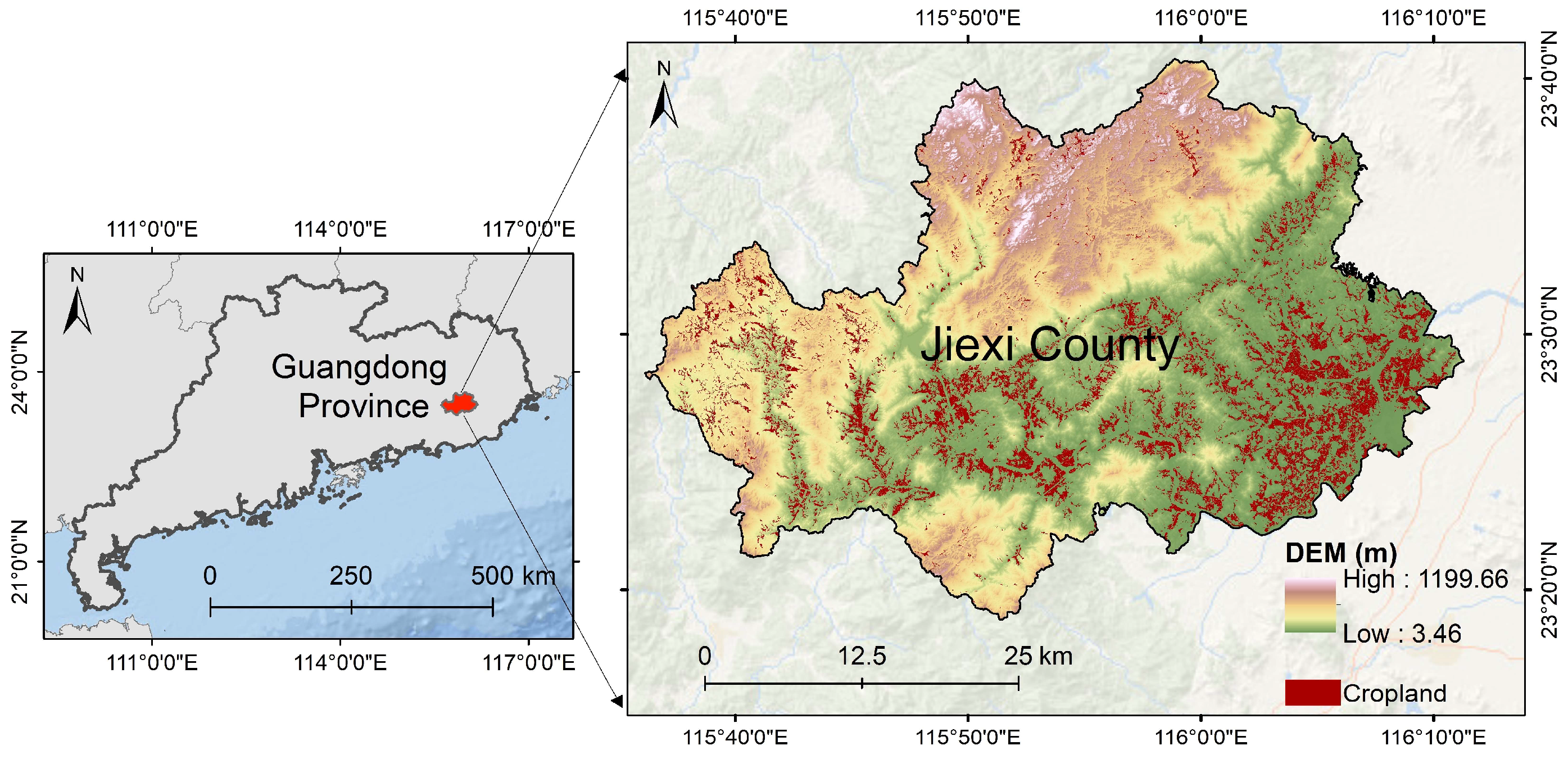
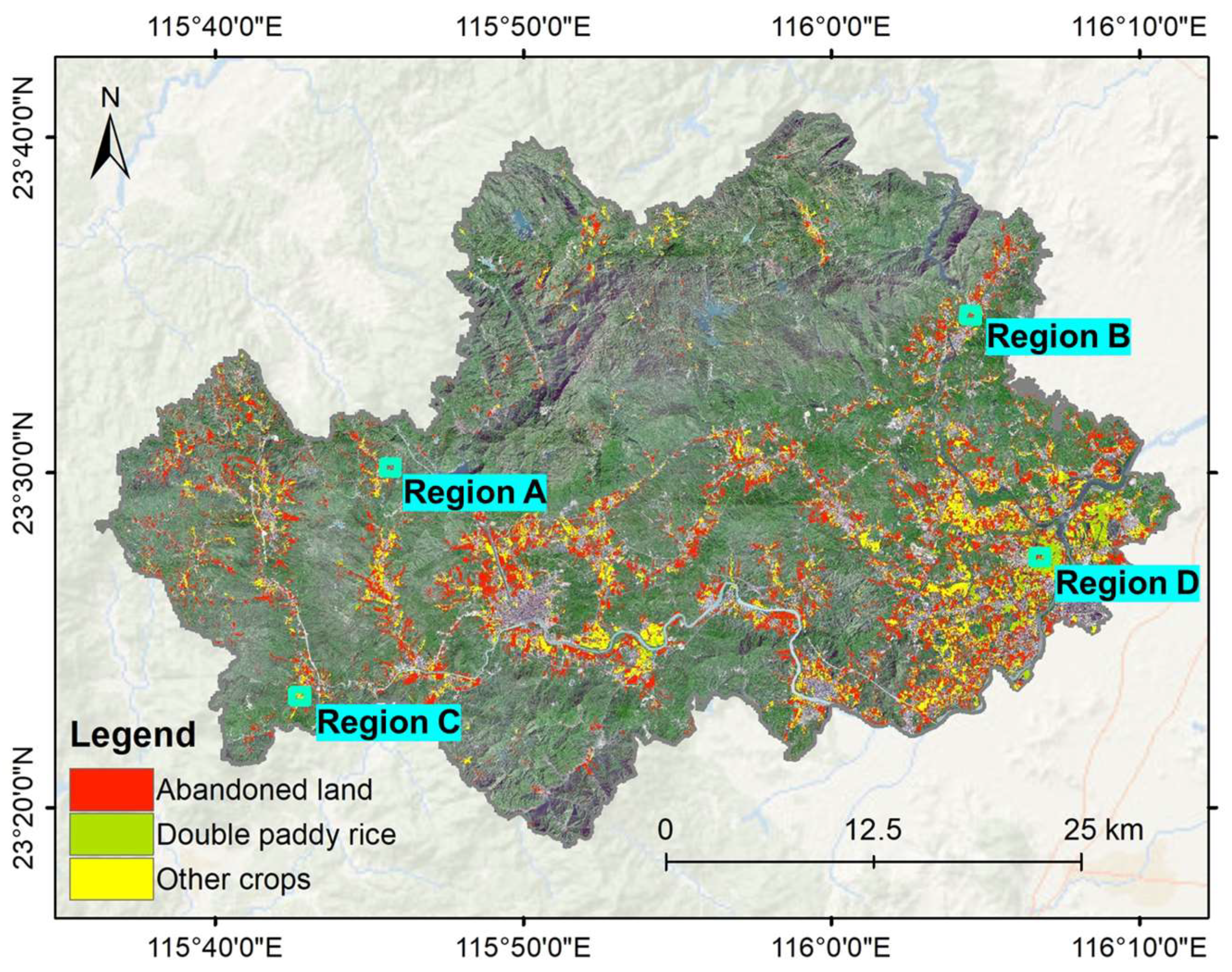
2.1. Study Area
2.2. Satellite Imagery
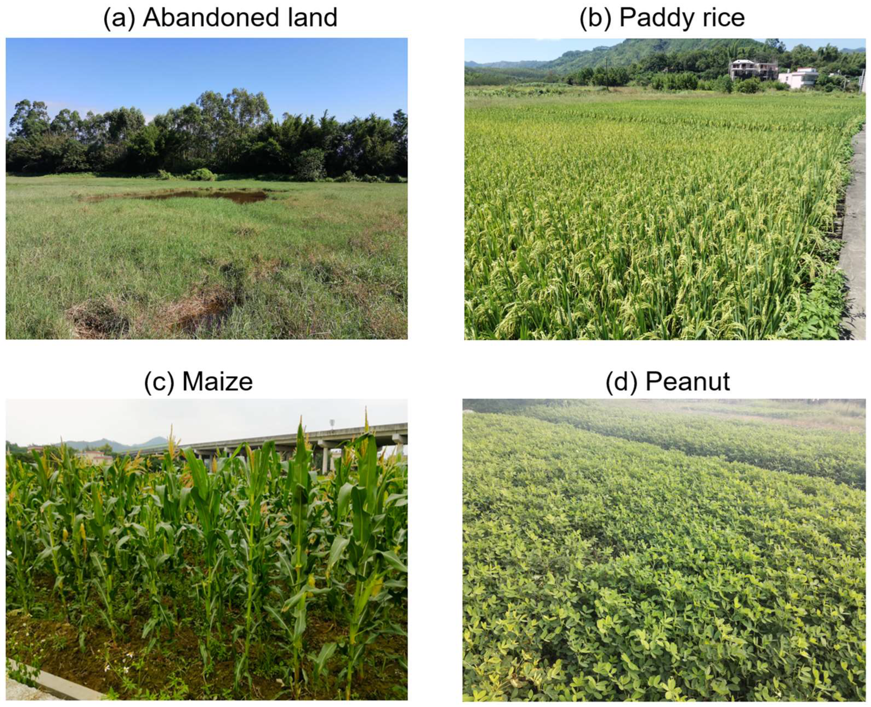
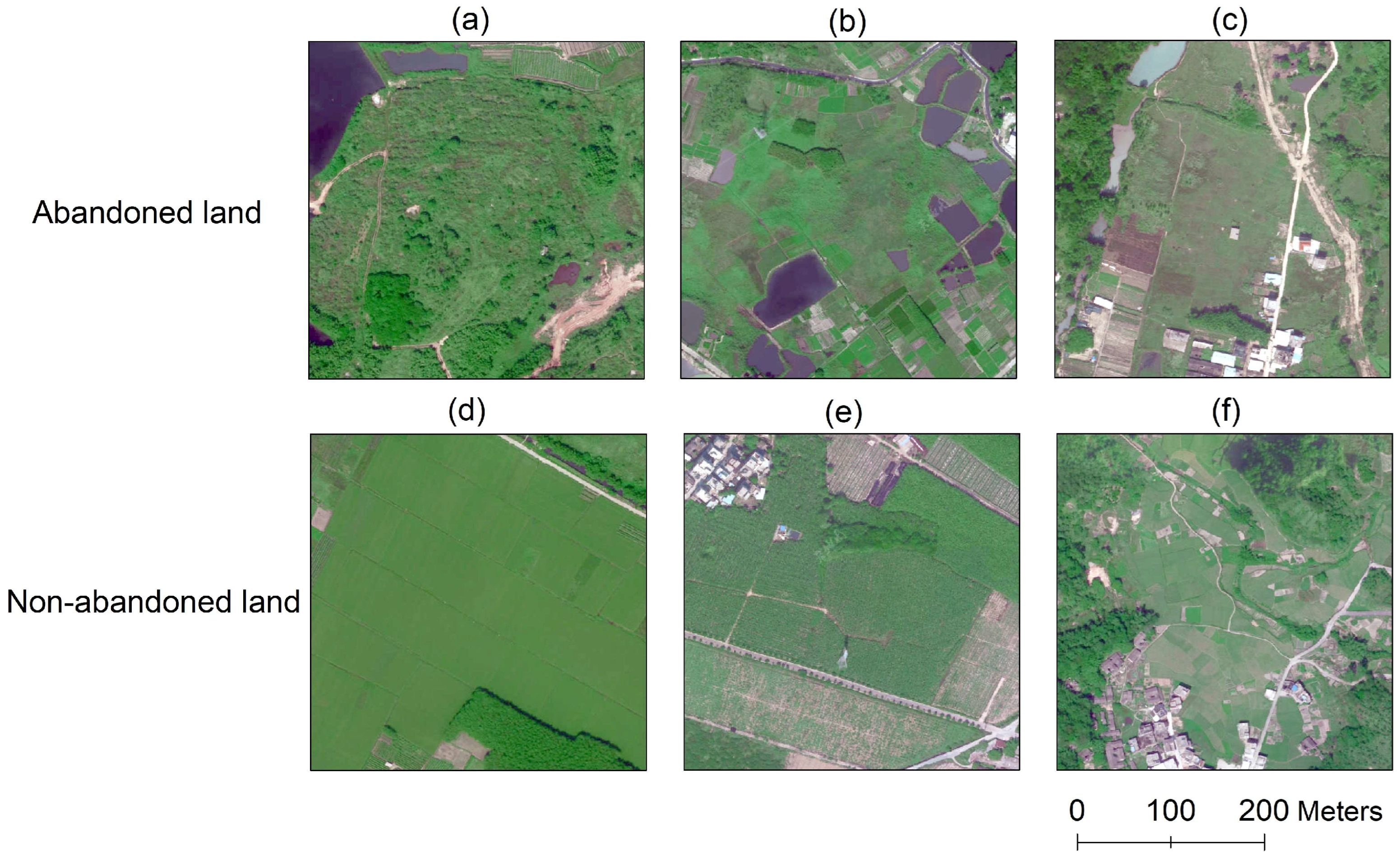
2.3. Sample Data Collection
2.4. Farmland Parcel Data
3. Methods
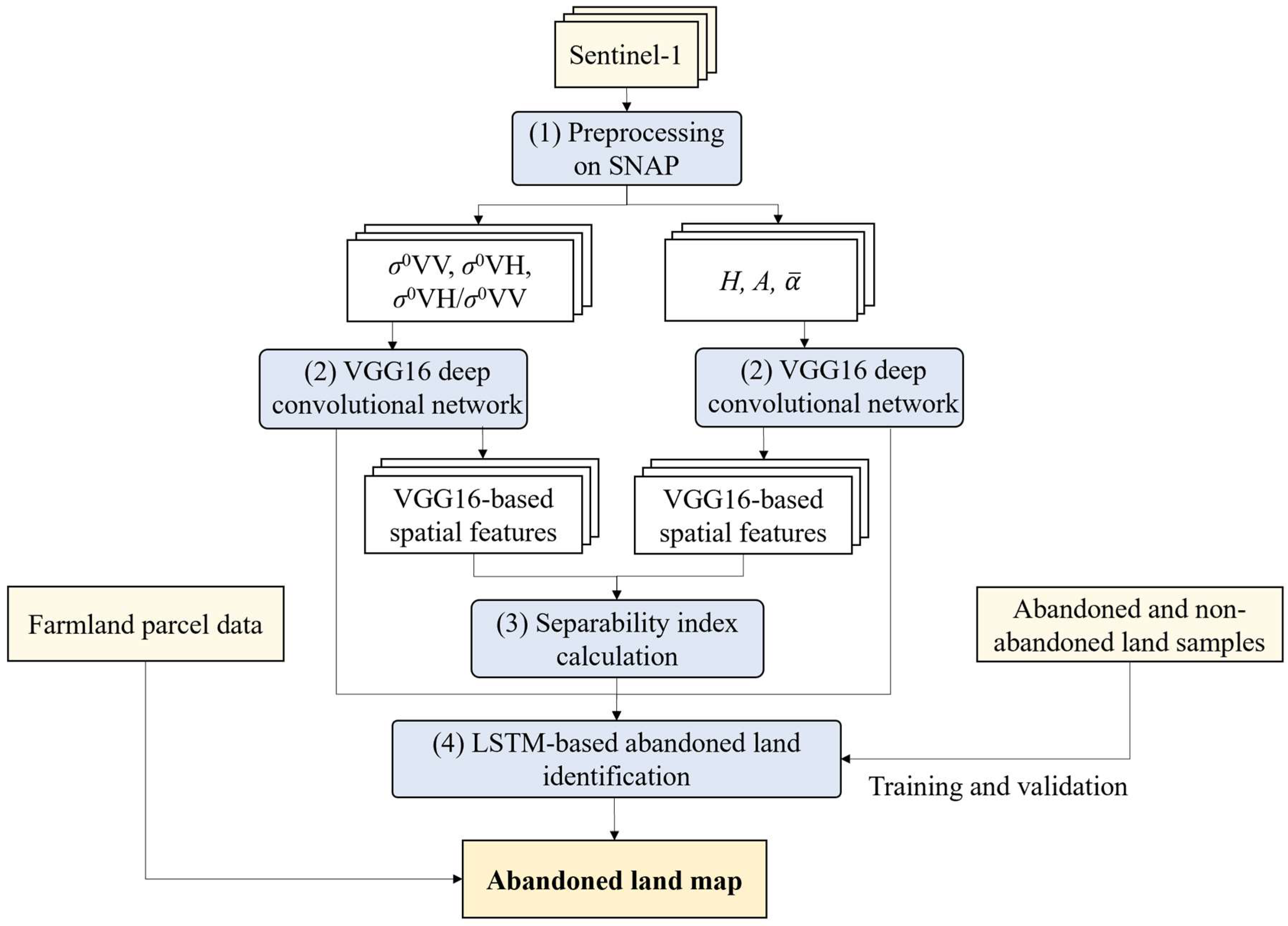
3.1. Sentinel-1 SLC Data Preprocessing
3.1.1. Backscattering Coefficients
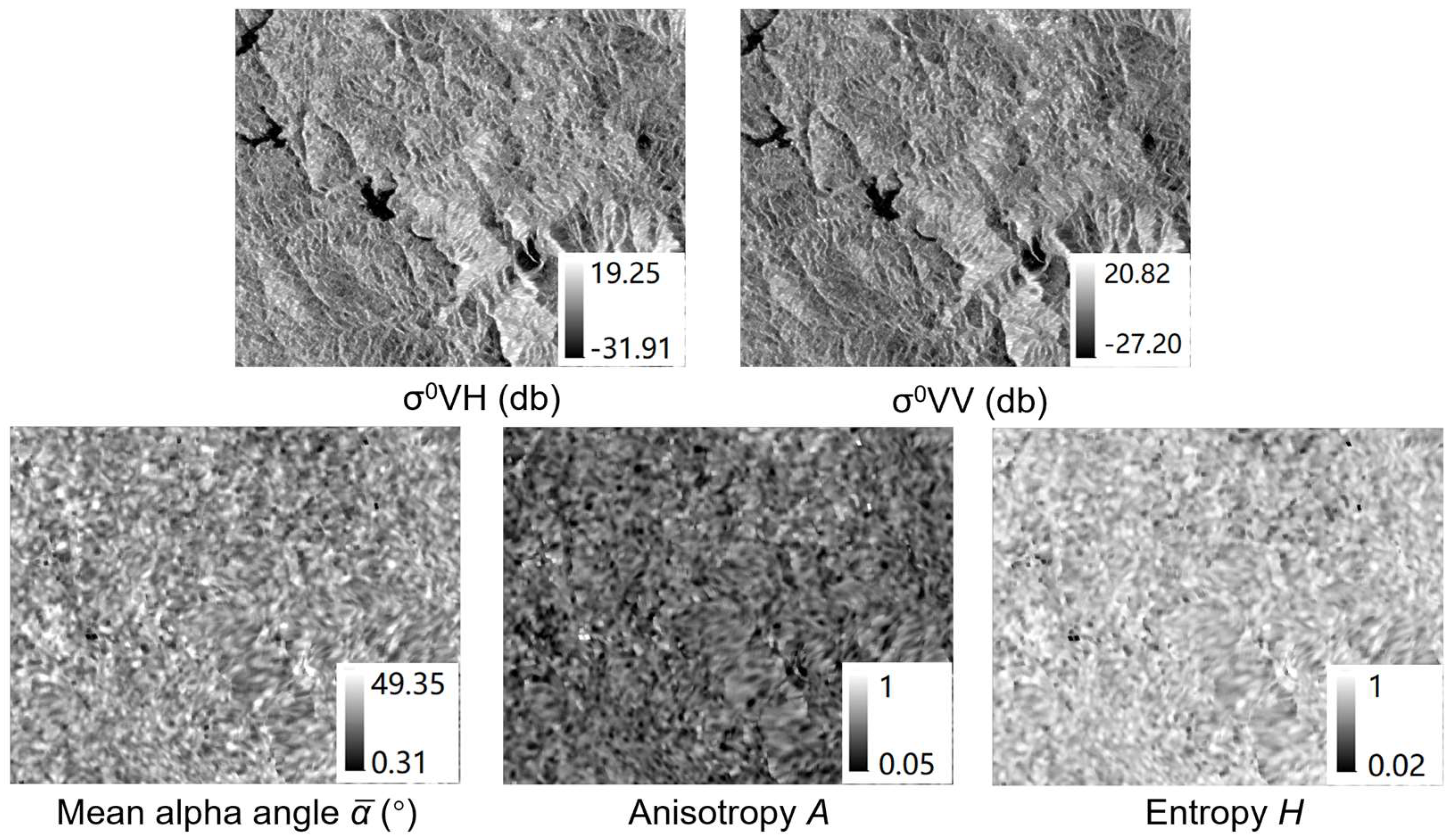
3.1.2. Polarimetric Parameters
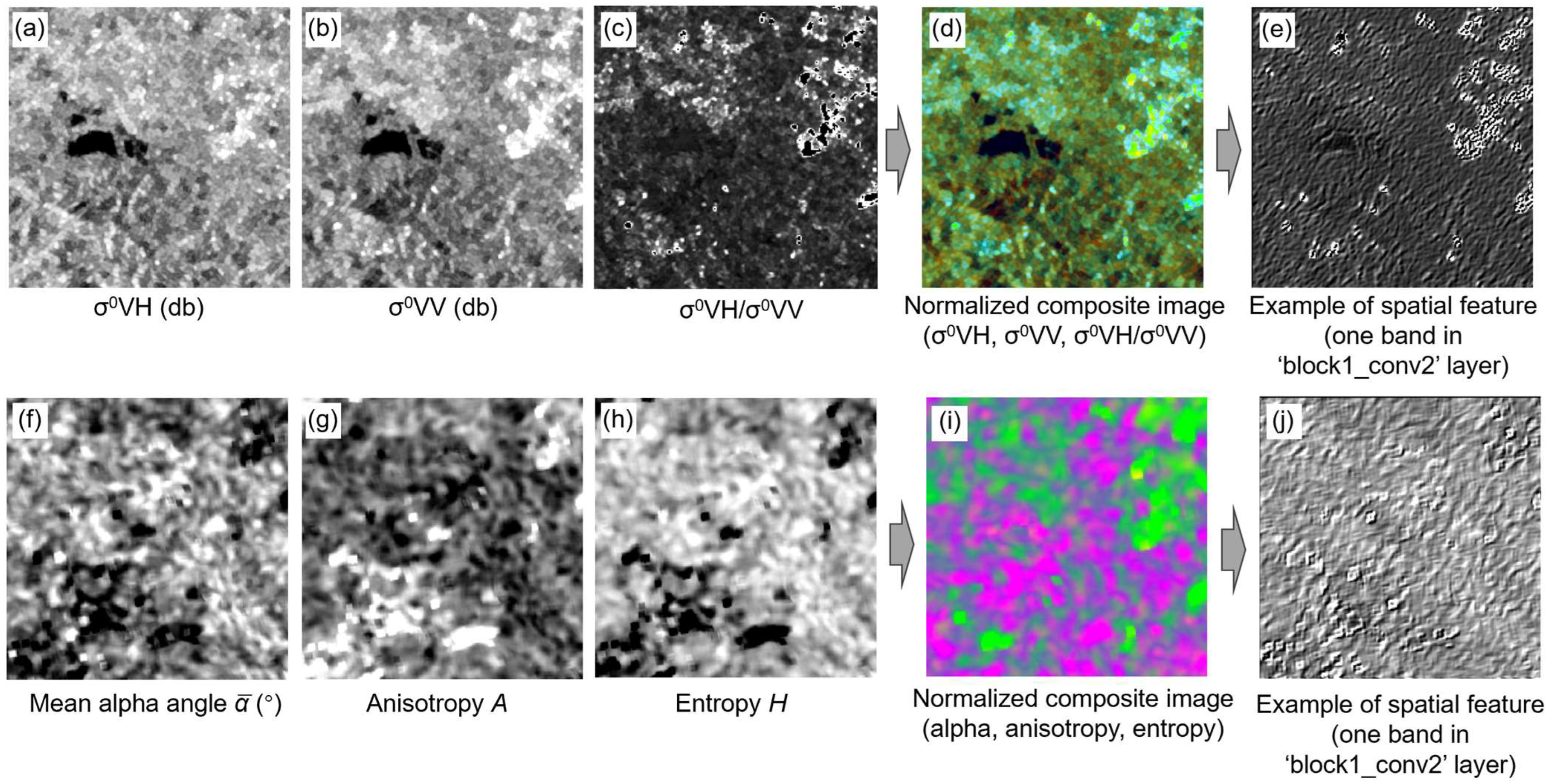
3.2. Spatial Feature Generation by VGG16 Network
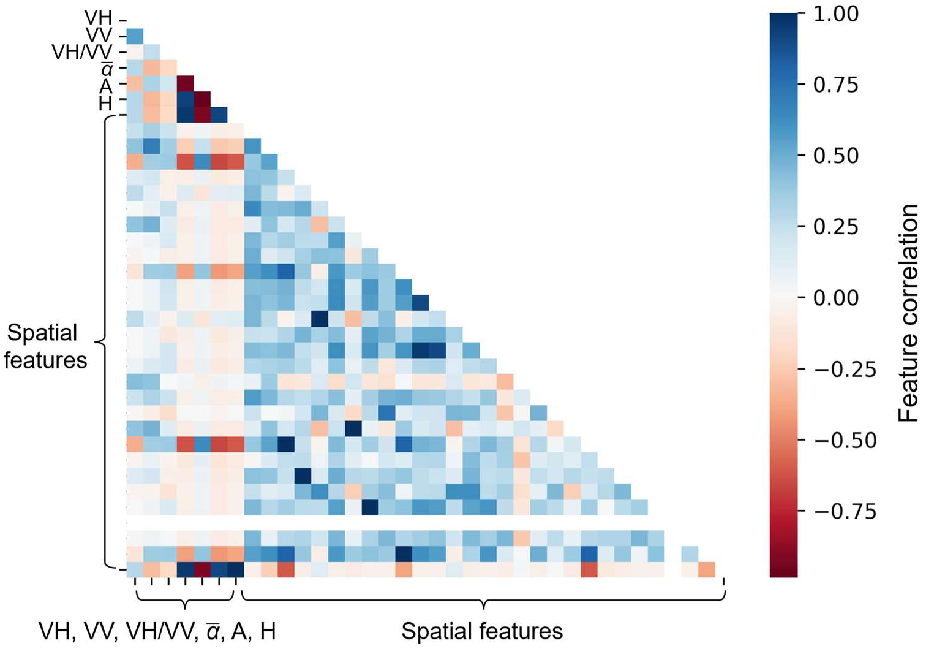
3.3. Effective Spatial Feature Selection by Separability Index
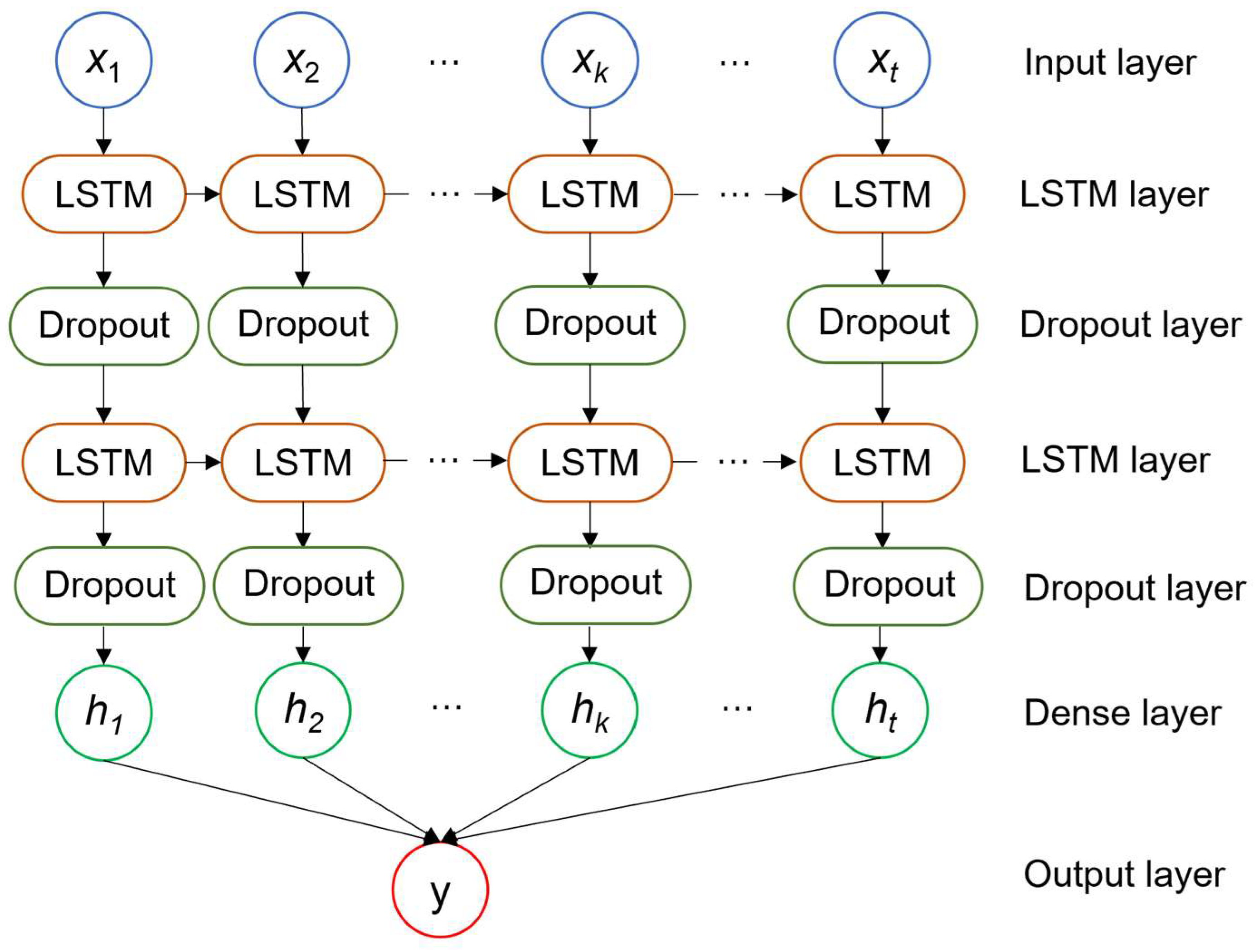
3.4. LSTM-Based Abandoned Land Identification
4. Results and Discussion
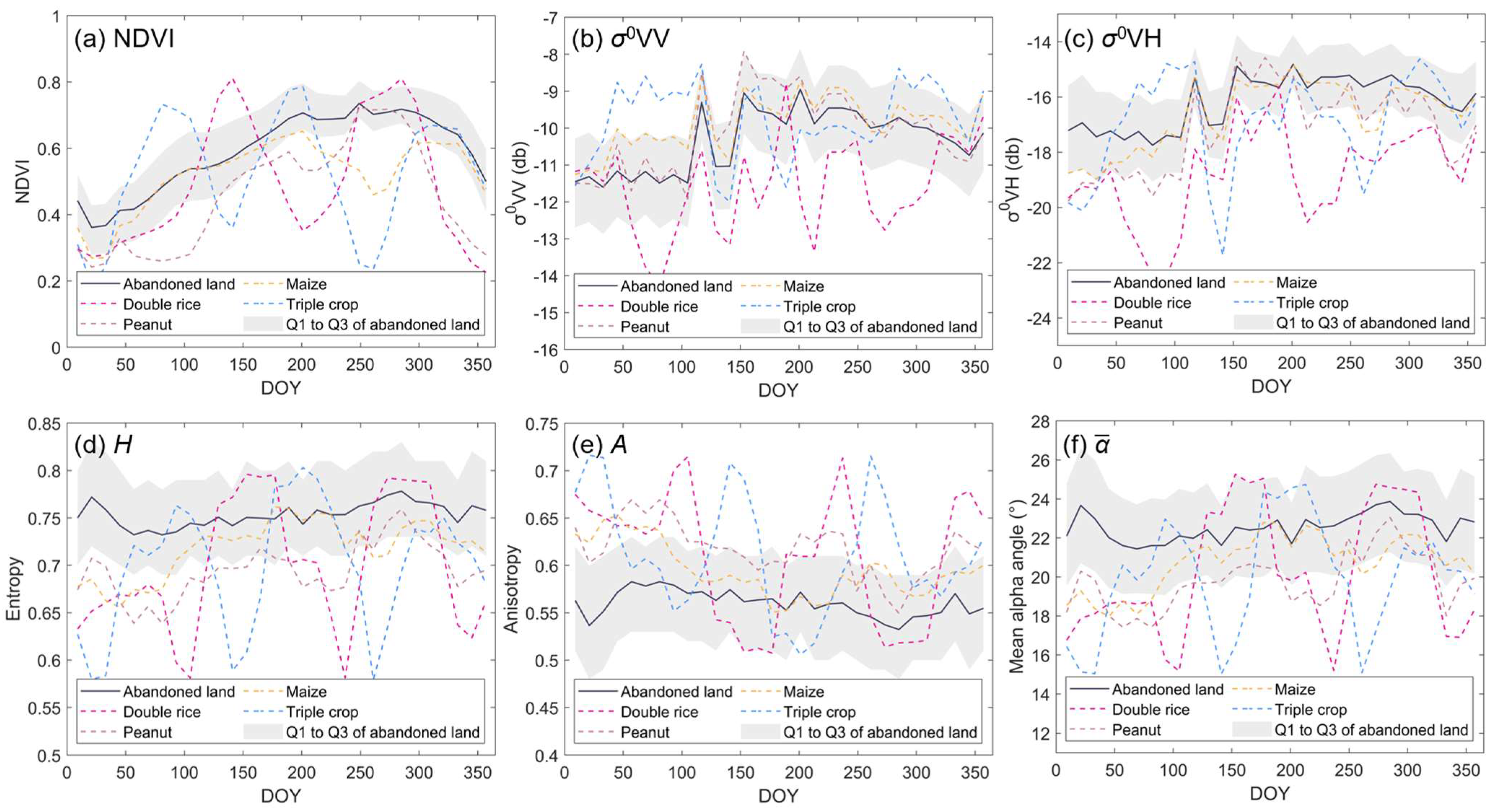
4.1. Temporal Profiles of Features for Abandoned Land and Crops
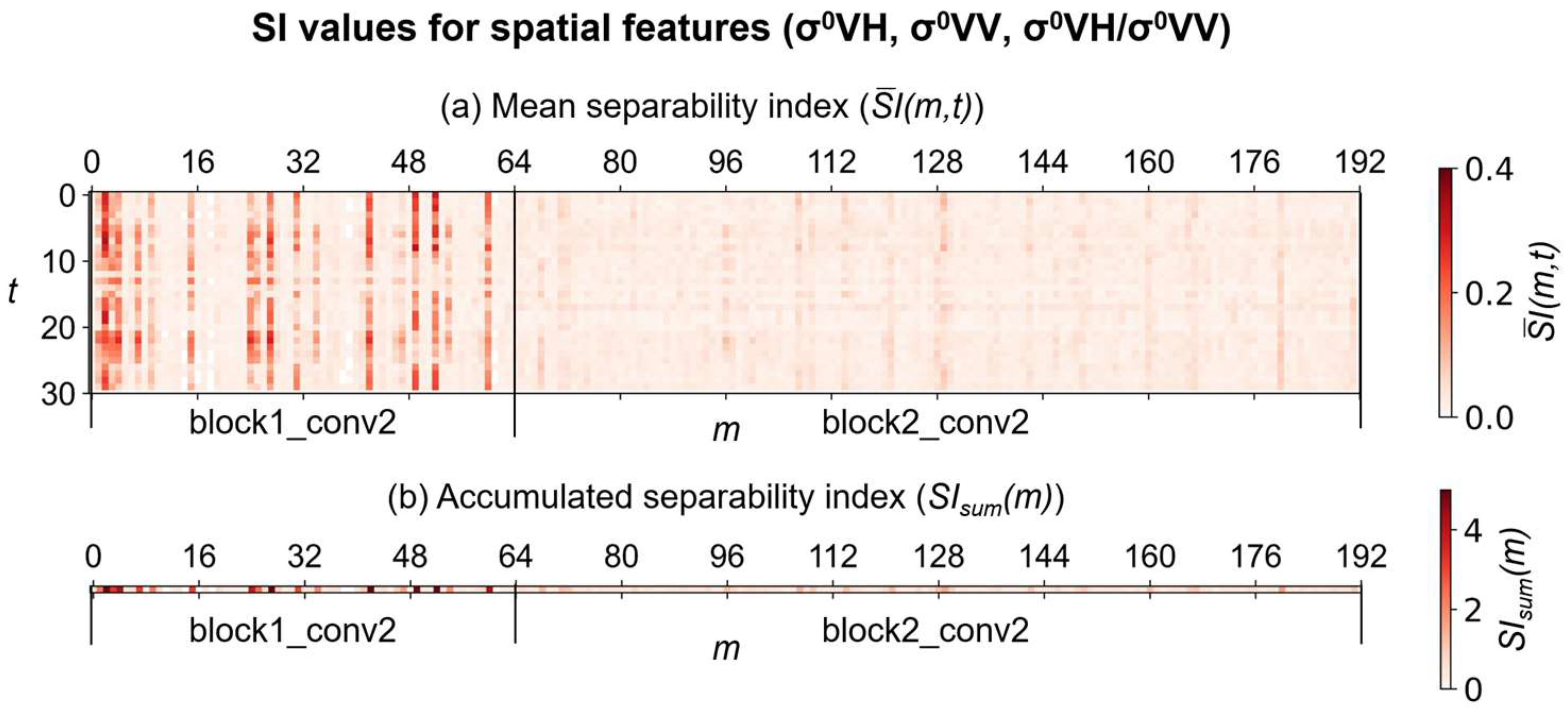
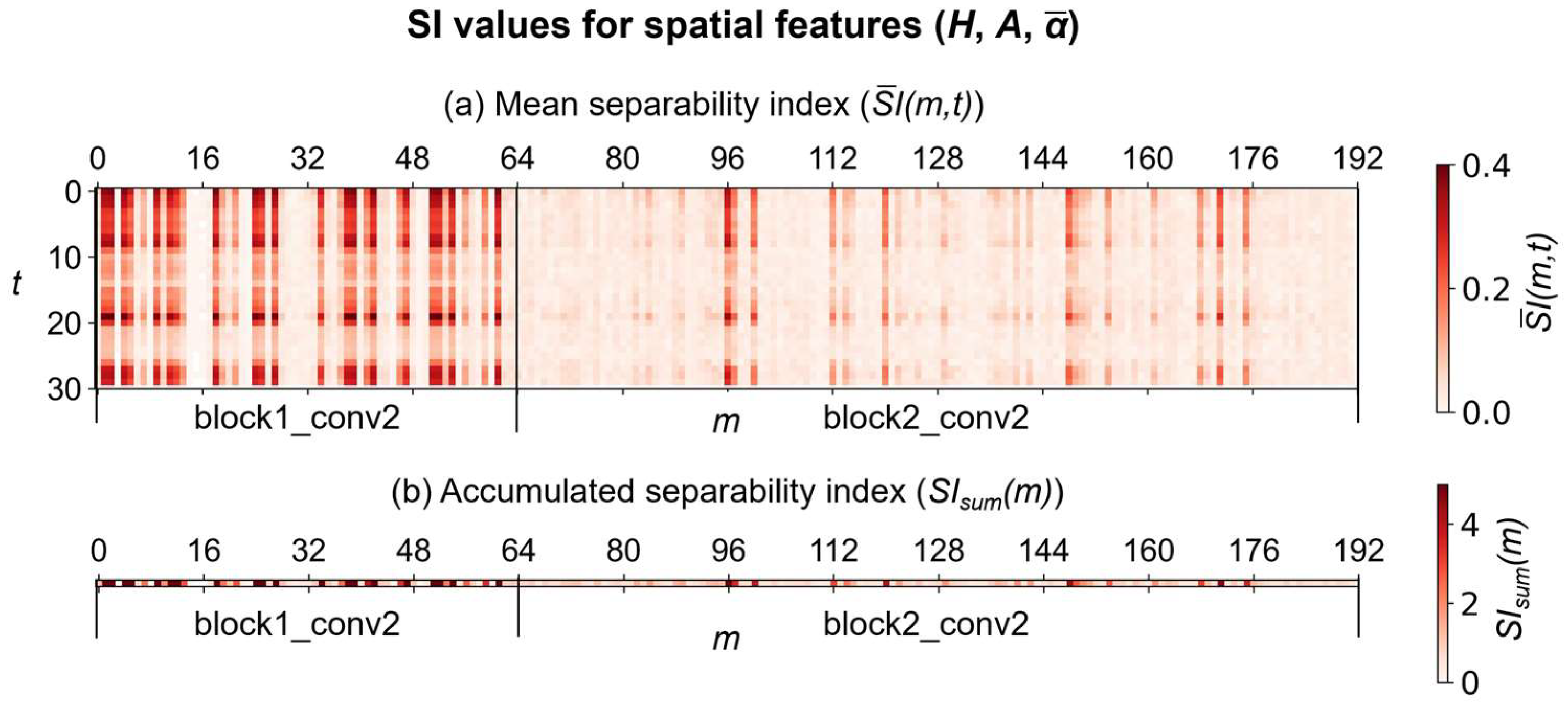
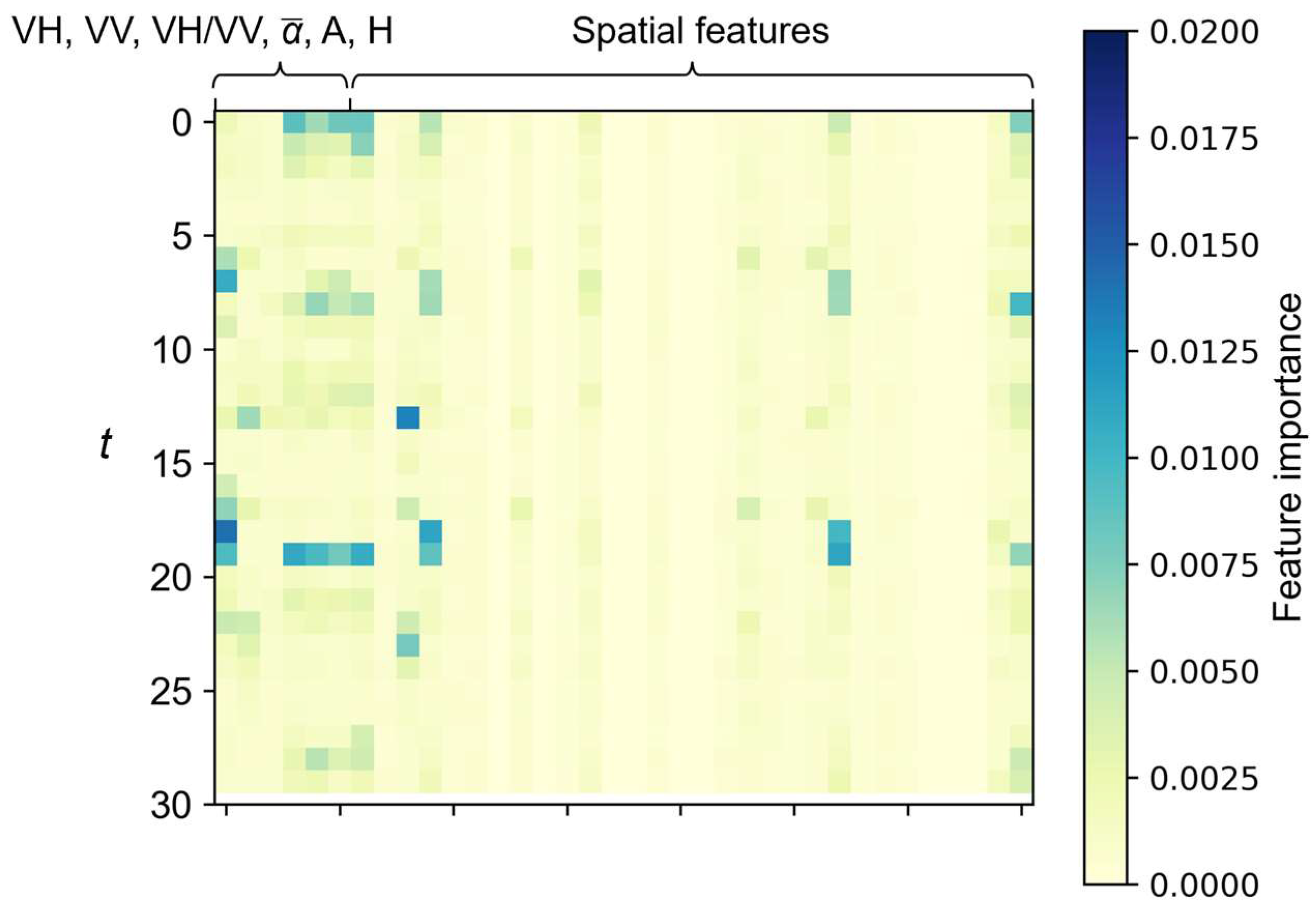
4.2. Optimal VGG16-Based Spatial Features
4.3. Accuracy Comparison Based on Different Feature Combinations
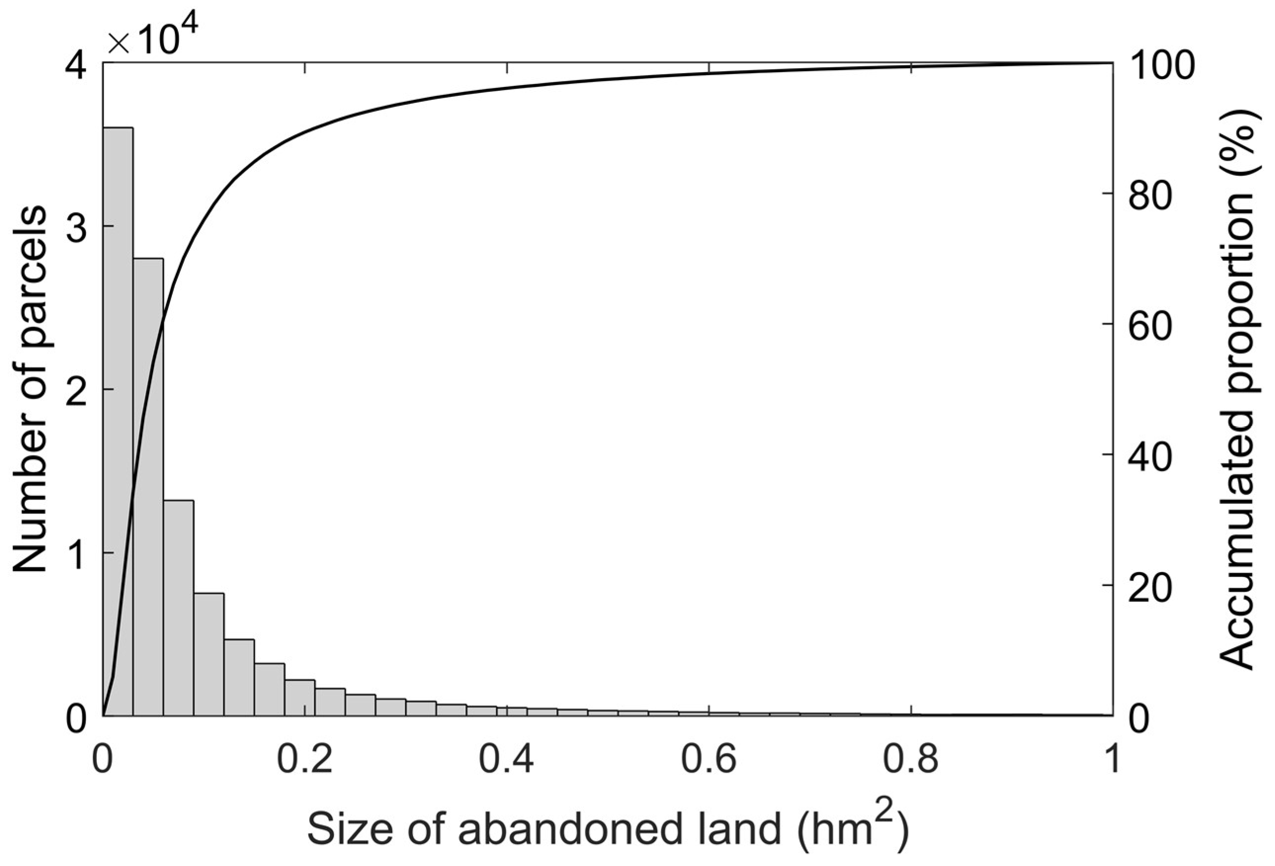
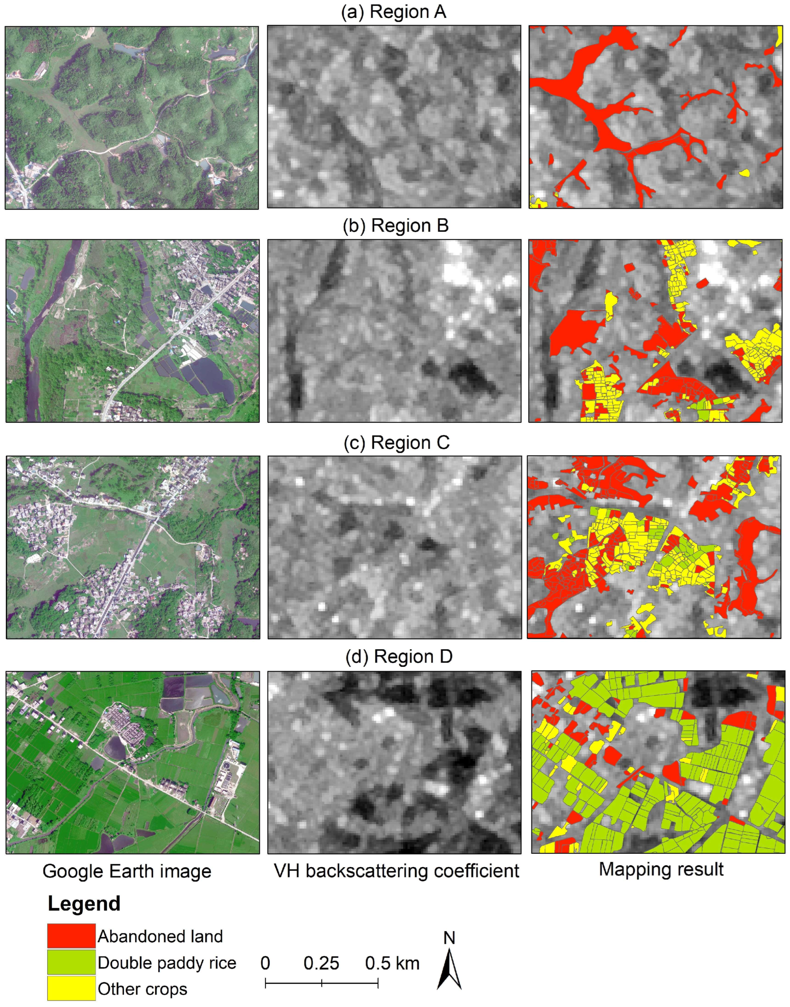
4.4. Mapping of Abandoned Land in Jiexi County
4.5. Discussion of the Computational Cost
5. Conclusions
Author Contributions
Funding
Conflicts of Interest
Appendix A


References
- Kuemmerle, T.; Radeloff, V.C.; Perzanowski, K.; Hostert, P. Cross-border comparison of land cover and landscape pattern in Eastern Europe using a hybrid classification technique. Remote Sens. Environ. 2006, 103, 449–464. [Google Scholar] [CrossRef]
- Aide, T.M.; Grau, H.R. Globalization, migration, and Latin American ecosystems. Science 2004, 305, 1915–1916. [Google Scholar] [CrossRef]
- Cramer, V.A.; Hobbs, R.J.; Standish, R.J. What’s new about old fields? Land abandonment and ecosystem assembly. Trends Ecol. Evol. 2008, 23, 104–112. [Google Scholar] [CrossRef]
- Ruiz-Flan˜o, P.; Garci´a-Ruiz, J.M.; Ortigosa, L. Geomorphological evolution of abandoned fields. A case study in the Central Pyrenees. CATENA 1992, 19, 301–308. [Google Scholar] [CrossRef]
- Stanchi, S.; Freppaz, M.; Agnelli, A.; Reinsch, T.; Zanini, E. Properties, best management practices and conservation of terraced soils in Southern Europe (from Mediterranean areas to the Alps): A review. Quat. Int. 2012, 265, 90–100. [Google Scholar] [CrossRef] [Green Version]
- Fischer, J.; Hartel, T.; Kuemmerle, T. Conservation policy in traditional farming landscapes. Conserv. Lett. 2012, 5, 167–175. [Google Scholar] [CrossRef] [Green Version]
- Meijninger, W.; Elbersen, B.; van Eupen, M.; Mantel, S.; Ciria, P.; Parenti, A.; Sanz, M.; Ortiz, P.; Acciai, M.; Monti, A. Identification of early abandonment in cropland through radar-based coherence data and application of a Random-Forest model. GCB Bioenergy 2022, 14, 735–755. [Google Scholar] [CrossRef]
- Goga, T.; Feranec, J.; Bucha, T.; Rusnák, M.; Sačkov, I.; Barka, I.; Kopecká, M.; Papčo, J.; Oťaheľ, J.; Szatmári, D.; et al. A review of the application of remote sensing data for abandoned agricultural land identification with focus on central and eastern Europe. Remote Sens. 2019, 11, 2759. [Google Scholar] [CrossRef] [Green Version]
- Yusoff, N.M.; Muharam, F.M.; Khairunniza-Bejo, S. Towards the use of remote-sensing data for monitoring of abandoned oil palm lands in Malaysia: A semi-automatic approach. Int. J. Remote Sens. 2017, 38, 432–449. [Google Scholar] [CrossRef]
- Prishchepov, A.V.; Radeloff, V.C.; Dubinin, M.; Alcantara, C. The effect of Landsat ETM/ETM+ image acquisition dates on the detection of agricultural land abandonment in Eastern Europe. Remote Sens. Environ. 2012, 126, 195–209. [Google Scholar] [CrossRef]
- Alcantara, C.; Kuemmerle, T.; Prishchepov, A.V.; Radeloff, V.C. Mapping abandoned agriculture with multi-temporal MODIS satellite data. Remote Sens. Environ. 2012, 124, 334–347. [Google Scholar] [CrossRef]
- Estel, S.; Kuemmerle, T.; Alcántara, C.; Levers, C.; Prishchepov, A.; Hostert, P. Mapping farmland abandonment and recultivation across Europe using MODIS NDVI time series. Remote Sens. Environ. 2015, 163, 312–325. [Google Scholar] [CrossRef]
- Wei, Z.; Gu, X.; Sun, Q.; Hu, X.; Gao, Y. Analysis of the Spatial and Temporal Pattern of Changes in Abandoned Farmland Based on Long Time Series of Remote Sensing Data. Remote Sens. 2021, 13, 2549. [Google Scholar] [CrossRef]
- Löw, F.; Fliemann, E.; Abdullaev, I.; Conrad, C.; Lamers, J.P.A. Mapping abandoned agricultural land in Kyzyl-Orda, Kazakhstan using satellite remote sensing. Appl. Geogr. 2015, 62, 377–390. [Google Scholar] [CrossRef]
- Wang, C.; Gao, Q.; Wang, X.; Yu, M. Spatially differentiated trends in urbanization, agricultural land abandonment and reclamation, and woodland recovery in Northern China. Sci. Rep. 2016, 6, 37658. [Google Scholar] [CrossRef] [PubMed] [Green Version]
- Dara, A.; Baumann, M.; Kuemmerle, T.; Pflugmacher, D.; Rabe, A.; Griffiths, P.; Hölzel, N.; Kamp, J.; Freitag, M.; Hostert, P. Mapping the timing of cropland abandonment and recultivation in northern Kazakhstan using annual Landsat time series. Remote Sens. Environ. 2018, 213, 49–60. [Google Scholar] [CrossRef]
- Campbell, J.E.; Lobell, D.B.; Genova, R.C.; Field, C.B. The global potential of bioenergy on abandoned agriculture lands. Environ. Sci. Technol. 2008, 42, 5791–5794. [Google Scholar] [CrossRef]
- Zhang, M.; Li, G.; He, T.; Zhai, G.; Guo, A.; Chen, H.; Wu, C. Reveal the severe spatial and temporal patterns of abandoned cropland in China over the past 30 years. Sci. Total Environ. 2023, 857, 159591. [Google Scholar] [CrossRef]
- Yin, H.; Prishchepov, A.V.; Kuemmerle, T.; Bleyhl, B.; Buchner, J.; Radeloff, V.C. Mapping agricultural land abandonment from spatial and temporal segmentation of Landsat time series. Remote Sens. Environ. 2018, 210, 12–24. [Google Scholar] [CrossRef]
- Olsen, V.M.; Fensholt, R.; Olofsson, P.; Bonifacio, R.; Butsic, V.; Druce, D.; Ray, D.; Prishchepov, A.V. The impact of conflict-driven cropland abandonment on food insecurity in South Sudan revealed using satellite remote sensing. Nat. Food 2021, 2, 990–996. [Google Scholar] [CrossRef]
- Witmer, F.D.W. Detecting war-induced abandoned agricultural land in northeast Bosnia using multispectral, multitemporal Landsat TM imagery. Int. J. Remote Sens. 2008, 29, 3805–3831. [Google Scholar] [CrossRef]
- Milenov, P.; Vassilev, V.; Vassileva, A.; Radkov, R.; Samoungi, V.; Dimitrov, Z.; Vichev, N. Monitoring of the risk of farmland abandonment as an efficient tool to assess the environmental and socio-economic impact of the Common Agriculture Policy. Int. J. Appl. Earth Obs. Geoinf. 2014, 32, 218–227. [Google Scholar] [CrossRef]
- Waske, B.; Braun, M. Classifier ensembles for land cover mapping using multitemporal SAR imagery. ISPRS J. Photogramm. Remote Sens. 2009, 64, 450–457. [Google Scholar] [CrossRef]
- Pohl, C.; Van Genderen, J.L. Review article multisensor image fusion in remote sensing: Concepts, methods and applications. Int. J. Remote Sens. 1998, 19, 823–854. [Google Scholar] [CrossRef] [Green Version]
- Stefanski, J.; Kuemmerle, T.; Chaskovskyy, O.; Griffiths, P.; Havryluk, V.; Knorn, J.; Korol, N.; Sieber, A.; Waske, B. Mapping land management regimes in Western Ukraine using optical and SAR data. Remote Sens. 2014, 6, 5279–5305. [Google Scholar] [CrossRef] [Green Version]
- Ray, T.W.; Farr, T.G.; van Zyl, J.J. Detection of land degradation with polarimetric SAR. Geophys. Res. Lett. 1992, 19, 1587–1590. [Google Scholar] [CrossRef]
- McNairn, H.; Champagne, C.; Shang, J.; Holmstrom, D.; Reichert, G. Integration of optical and Synthetic Aperture Radar (SAR) imagery for delivering operational annual crop inventories. ISPRS J. Photogramm. Remote Sens. 2009, 64, 434–449. [Google Scholar] [CrossRef]
- Yusoff, N.M.; Muharam, F.M.; Takeuchi, W.; Darmawan, S.; Abd Razak, M.H. Phenology and classification of abandoned agricultural land based on ALOS-1 and 2 PALSAR multi-temporal measurements. Int. J. Digit. Earth 2017, 10, 155–174. [Google Scholar] [CrossRef]
- Xie, Q.; Wang, J.; Liao, C.; Shang, J.; Lopez-Sanchez, J.M.; Fu, H.; Liu, X. On the use of Neumann Decomposition for crop classification using multi-temporal RADARSAT-2 polarimetric SAR data. Remote Sens. 2019, 11, 776. [Google Scholar] [CrossRef] [Green Version]
- Ioannidou, M.; Koukos, A.; Sitokonstantinou, V.; Papoutsis, I.; Kontoes, C. Assessing the added value of Sentinel-1 PolSAR data for crop classification. Remote Sens. 2022, 14, 5739. [Google Scholar] [CrossRef]
- Canisius, F.; Shang, J.; Liu, J.; Huang, X.; Ma, B.; Jiao, X.; Geng, X.; Kovacs, J.M.; Walters, D. Tracking crop phenological development using multi-temporal polarimetric Radarsat-2 data. Remote Sens. Environ. 2018, 210, 508–518. [Google Scholar] [CrossRef]
- Zhou, Y.n.; Luo, J.; Feng, L.; Zhou, X. DCN-Based spatial features for improving parcel-based crop classification using high-resolution optical images and multi-temporal SAR data. Remote Sens. 2019, 11, 1619. [Google Scholar]
- Kussul, N.; Lavreniuk, M.; Skakun, S.; Shelestov, A. Deep learning classification of land cover and crop types using remote sensing data. IEEE Geosci. Remote Sens. Lett. 2017, 14, 778–782. [Google Scholar] [CrossRef]
- Zhang, C.; Sargent, I.; Pan, X.; Li, H.; Gardiner, A.; Hare, J.; Atkinson, P.M. Joint deep learning for land cover and land use classification. Remote Sens. Environ. 2019, 221, 173–187. [Google Scholar] [CrossRef] [Green Version]
- Li, Y.; Peng, C.; Chen, Y.; Jiao, L.; Zhou, L.; Shang, R. A deep learning method for change detection in synthetic aperture radar images. IEEE Trans. Geosci. Remote Sens. 2019, 57, 5751–5763. [Google Scholar] [CrossRef]
- Cloude, S.R.; Pottier, E. An entropy based classification scheme for land applications of polarimetric SAR. IEEE Trans. Geosci. Remote Sens. 1997, 35, 68–78. [Google Scholar] [CrossRef]
- Simonyan, K.; Zisserman, A. Very Deep Convolutional Networks for Large-Scale Image Recognition. In Proceedings of the ICLR 2015, San Diego, CA, USA, 7–9 May 2015. [Google Scholar]
- Liu, X.; Chi, M.; Zhang, Y.; Qin, Y. Classifying high resolution remote sensing images by fine-tuned VGG deep networks. In Proceedings of the IGARSS 2018—2018 IEEE International Geoscience and Remote Sensing Symposium, Valencia, Spain, 22–27 July 2018; pp. 7137–7140. [Google Scholar]
- Mu, Y.; Ni, R.; Zhang, C.; Gong, H.; Hu, T.; Li, S.; Sun, Y.; Zhang, T.; Guo, Y. A lightweight model of VGG-16 for remote sensing image classification. IEEE J. Sel. Top. Appl. Earth Obs. Remote Sens. 2021, 14, 6916–6922. [Google Scholar] [CrossRef]
- Somers, B.; Asner, G.P. Multi-temporal hyperspectral mixture analysis and feature selection for invasive species mapping in rainforests. Remote Sens. Environ. 2013, 136, 14–27. [Google Scholar] [CrossRef]
- Hu, Q.; Sulla-Menashe, D.; Xu, B.; Yin, H.; Tang, H.; Yang, P.; Wu, W. A phenology-based spectral and temporal feature selection method for crop mapping from satellite time series. Int. J. Appl. Earth Obs. Geoinf. 2019, 80, 218–229. [Google Scholar] [CrossRef]
- Hochreiter, S.; Schmidhuber, J. Long short-term memory. Neural Comput. 1997, 9, 1735–1780. [Google Scholar] [CrossRef]
- Tian, H.; Wang, P.; Tansey, K.; Zhang, J.; Zhang, S.; Li, H. An LSTM neural network for improving wheat yield estimates by integrating remote sensing data and meteorological data in the Guanzhong Plain, PR China. Agric. For. Meteorol. 2021, 310, 108629. [Google Scholar] [CrossRef]
- Portalés-Julià, E.; Campos-Taberner, M.; García-Haro, F.; Gilabert, M.A. Assessing the Sentinel-2 Capabilities to Identify Abandoned Crops Using Deep Learning. Agronomy 2021, 11, 654. [Google Scholar] [CrossRef]


| Date | Date | ||
|---|---|---|---|
| 1 | 9 January 2021 | 16 | 8 July 2021 |
| 2 | 21 January 2021 | 17 | 20 July 2021 |
| 3 | 2 February 2021 | 18 | 1 August 2021 |
| 4 | 14 February 2021 | 19 | 13 August 2021 |
| 5 | 26 February 2021 | 20 | 25 August 2021 |
| 6 | 10 March 2021 | 21 | 6 September 2021 |
| 7 | 22 March 2021 | 22 | 18 September 2021 |
| 8 | 3 April 2021 | 23 | 30 September 2021 |
| 9 | 15 April 2021 | 24 | 12 October 2021 |
| 10 | 27 April 2021 | 25 | 24 October 2021 |
| 11 | 9 May 2021 | 26 | 5 November 2021 |
| 12 | 21 May 2021 | 27 | 17 November 2021 |
| 13 | 2 June 2021 | 28 | 29 November 2021 |
| 14 | 14 June 2021 | 29 | 11 December 2021 |
| 15 | 26 June 2021 | 30 | 23 December 2021 |
| Feature Combination | Reference | Classification | PA | ||
|---|---|---|---|---|---|
| Abandoned Land | Double Rice | Other Crops | |||
| σ0VH, σ0VV, σ0VH/σ0VV | Abandoned land | 598 | 22 | 89 | 84.34% |
| Double rice | 14 | 541 | 68 | 86.84% | |
| Other crops | 136 | 62 | 369 | 65.08% | |
| UA | 79.95% | 86.56% | 70.15% | ||
| OA: 79.41%, Kappa: 0.69 | |||||
| H, A, | Abandoned land | 608 | 6 | 95 | 85.75% |
| Double rice | 17 | 540 | 66 | 86.68% | |
| Other crops | 128 | 66 | 373 | 65.78% | |
| UA | 80.74% | 88.24% | 69.85% | ||
| OA: 80.09%, Kappa: 0.70 | |||||
| σ0VH, σ0VV, σ0VH/σ0VV, H, A, | Abandoned land | 616 | 9 | 84 | 86.88% |
| Double rice | 16 | 550 | 57 | 88.28% | |
| Other crops | 103 | 54 | 410 | 72.31% | |
| UA | 83.81% | 89.72% | 74.41% | ||
| OA: 82.99%, Kappa: 0.74 | |||||
| σ0VH, σ0VV, σ0VH/σ0VV, VGG16-based spatial features | Abandoned land | 615 | 16 | 78 | 86.74% |
| Double rice | 12 | 542 | 69 | 87.00% | |
| Other crops | 117 | 61 | 389 | 68.61% | |
| UA | 82.66% | 87.56% | 72.57% | ||
| OA: 81.41%, Kappa: 0.72 | |||||
| σ0VH, σ0VV, σ0VH/σ0VV, H, A, , VGG16-based spatial features | Abandoned land | 626 | 18 | 65 | 88.29% |
| Double rice | 15 | 556 | 52 | 89.25% | |
| Other crops | 104 | 71 | 392 | 69.14% | |
| UA | 84.03% | 86.20% | 77.01% | ||
| OA: 82.89%, Kappa: 0.74 | |||||
Disclaimer/Publisher’s Note: The statements, opinions and data contained in all publications are solely those of the individual author(s) and contributor(s) and not of MDPI and/or the editor(s). MDPI and/or the editor(s) disclaim responsibility for any injury to people or property resulting from any ideas, methods, instructions or products referred to in the content. |
© 2023 by the authors. Licensee MDPI, Basel, Switzerland. This article is an open access article distributed under the terms and conditions of the Creative Commons Attribution (CC BY) license (https://creativecommons.org/licenses/by/4.0/).
Share and Cite
Yang, Y.; Wu, Z.; Xiao, W.; Zhou, Y.; Huang, Q.; Wu, T.; Luo, J.; Wang, H. Abandoned Land Mapping Based on Spatiotemporal Features from PolSAR Data via Deep Learning Methods. Remote Sens. 2023, 15, 3942. https://doi.org/10.3390/rs15163942
Yang Y, Wu Z, Xiao W, Zhou Y, Huang Q, Wu T, Luo J, Wang H. Abandoned Land Mapping Based on Spatiotemporal Features from PolSAR Data via Deep Learning Methods. Remote Sensing. 2023; 15(16):3942. https://doi.org/10.3390/rs15163942
Chicago/Turabian StyleYang, Yingpin, Zhifeng Wu, Wenju Xiao, Ya’nan Zhou, Qiting Huang, Tianjun Wu, Jiancheng Luo, and Haiyun Wang. 2023. "Abandoned Land Mapping Based on Spatiotemporal Features from PolSAR Data via Deep Learning Methods" Remote Sensing 15, no. 16: 3942. https://doi.org/10.3390/rs15163942