Joint Posterior Probability Active Learning for Hyperspectral Image Classification

Abstract

Active learning (AL) is an approach that can reduce the dependence on the labeled set significantly. However, most current active-learning methods are only concerned with the first two columns of the posterior probability matrix during the sampling phase. When the difference between the first and second-largest posterior probabilities of several samples is proximate, these approaches fail to distinguish them further. To improve these deficiencies, we propose an active-learning algorithm, joint posterior probabilistic active learning combined with conditional random field (JPPAL_CRF). In the active-learning sampling phase, a new sampling decision function is built by jointing all the information in the posterior probability matrix. By doing so, the variability between different samples is refined, which makes the selected samples more meaningful for classification. Then, a conditional random field (CRF) approach is applied to mine the regional spatial information of the hyperspectral image and optimize the classification results. Experiments on two common hyperspectral datasets validate the effectiveness of JPPAL_CRF.

1. Introduction

Hyperspectral image (HSI) classification is a vibrant research area for the remote-sensing community and is essential in both civilian and military applications [1,2]. The most significant characteristic of HSI is the image-space spectrum integration. This includes not only spatial information but also tens or even hundreds of narrow spectral bands on the surface of Earth [3,4]. This characteristic provides the opportunity for precise classification of ground objects. However, it also results in the “Hughes phenomenon”. The high-dimensional-data nature of HSI reduces the accuracy of the classifier when the quantity of the training set is limited [5]. Therefore, the performance of supervised classification algorithms depends largely on the “quantity” and “quality” of the labeled set [6]. However, it is costly and tedious to obtain enough training samples with real labels in practice. Therefore, it is essential to design efficient algorithms that have both high classification accuracy and minimize training samples.

The approach to reduce computational and time costs by actively selecting the labeled set is called AL [7]. AL is a process of selecting the most valuable samples to expand the training set. This approach provides a good solution for situations where the size of the label set in the classification process is small [8]. Specifically, a small initial labeled set and a large unlabeled set are given. AL quantifies the informativeness of pixel-class labels by their uncertainty, and manually labels unlabeled samples where the uncertainty in the class labels is the greatest. The labeled samples are iteratively extended so that the labeled samples have the maximum amount of information. By intelligently selecting unlabeled samples instead of randomly selecting them, the classifier model is better trained to achieve better classification accuracy [9,10].

In general, according to the selection strategy of the unlabeled set, AL algorithms can be divided into two major types: committee learner-based approaches [11,12] and confidence-based approaches. The first labels the samples with various classifiers and then the oracle makes the final decision on the disputed labeled samples. The difference between the different classifiers is that they predict different results for the sample labels [13,14,15]. Committee learner-based approaches include querying by bagging [16], bagging entropy, and bottling normalized entropy. The latter is first given lower confidence samples by the classifier and then given to the oracle for selective labeling. Confidence-based approaches can be further divided into two broad types: Margin Sampling (MS)-based approaches [13,17] and class probability distribution-based approaches, also known as Breaking Ties (BT) [18]. MS considers the samples closest to the classifier separation hyperplane to be the most informative samples. BT considers the samples with the smallest difference between the two maximum posterior probabilities to be the samples with the highest uncertainty.

Among these active-learning approaches, class probability distribution-based approaches attract our attention. Most of them only consider the difference between the first two columns of the posterior probability matrix. BT tends to assume that two samples have the same amount of information when the difference between the first two columns of the posterior probability matrix is equal. Then, the sampling strategy is difficult to distinguish which sample is more important. To solve this problem, we propose a new active-learning algorithm, JPPAL_CRF. This approach mines all the information contained in the posterior probability matrix. This allows the difference between the samples to be further refined so that more suitable samples for training can be selected. In addition, to fully utilize the spatial information in the HSI, we optimize the classification result using CRF. The contributions of this letter can be summarized as follows:

• JPPAL_CRF focuses not only on the two maximum posterior probabilities but also on the contribution of the remaining posterior probabilities to the information content of the sample. By combining all obtained posterior probabilities to construct a sampling function, an AL strategy is proposed.
• The sampling process reduces the selection of labeled samples trapped at the boundary of a single class and focuses more on gaining more diversity during the sample selection process. It not only improves classification accuracy but also performs well in the balance of all classes.

The remainder of this paper is organized as follows. Section 2 describes the proposed approach. Section 3 demonstrates its effectiveness through experiments on two HSI datasets. Finally, Section 4 gives the conclusion.

2. Proposed Approach

This section presents the proposed AL algorithm, namely JPPAL_CRF, which is shown in the framework in Figure 1. The fundamental idea of the algorithm is to build a new active-learning model by joining all the posterior probabilities from the support vector machine (SVM). Then, CRF is utilized to mine the spatial information of the dataset and further optimize the classification results.

2.1. Sampling Strategy by Combining Posterior Probabilities

Let $\mathit{X}=\left\{{\mathit{x}}_{\mathbf{1}},\cdots \cdots ,{\mathit{x}}_{\mathit{n}}\right\}\in {\mathbb{R}}^{d\times n}$ be the HSI matrix, where d is the number of spectral bands, n is the total number of spatial pixels, and ${\mathit{x}}_{\mathit{i}}=\left\{x_{i1},x_{i2},\cdots \cdots ,x_{id}\right\}$ is a spectral vector. Let $\mathit{Y}=\left\{y_{1,}\cdots \cdots y_n\right\}\in {\mathbb{R}}^n$ be the label of the image where each element is one of the pre-defined classes, i.e., $y_i\in \mathrm{K}=\left\{1,\cdots \cdots K\right\}$.

BT depends on the minimum difference between the first two columns of the sample probability matrix [12]. The decision criterion is

$$\begin{array}{c}{\widehat{x}}_i^{BT}=\underset{{\mathit{x}}_{\mathit{i}}\in {\mathit{X}}_{\mathit{U}}}{argmin}\left\{\underset{k\in \mathrm{K}}{max}p(y_i=k|{\mathit{x}}_{\mathit{i}},\widehat{\omega })-\underset{k\in \mathrm{K}\setminus \left\{k+\right\}}{max}p(y_i=k|{\mathit{x}}_{\mathit{i}},\widehat{\omega })\right\},\end{array}$$

(1)

where $k+=arg{max}_{k\in \mathrm{K}}p(y_i=k\left|{\mathit{x}}_{\mathit{i}},\widehat{\omega }\right.)$ is the class label corresponding to the maximum posterior probability of $x_i$. $\mathrm{K}\setminus \left\{k+\right\}$ is the rest of the class labels except $k+$, ${\mathit{X}}_{\mathit{U}}$ is the unlabeled set, and $\widehat{\omega }$ is the logistic regressor set. From Equation (1), it can be observed that BT focuses on the area of the boundary between two classes, to obtain more diversity during the sample selection process [19].

With BT sampling, it is difficult to distinguish them when two samples have similar BT scores. For example, when the posterior probabilities of two samples are (0.4, 0.4, 0.2, 0) and (0.3, 0.3, 0.2, 0.2). We can hardly distinguish these two samples when relying only on the two maximum posterior probabilities to calculate the scores. However, it is an efficient solution to this problem by combining all the posterior probabilities to extend the difference between these samples. The decision criteria for the joint posterior probabilities is

$${\widehat{x}}_i^{JJP}=\underset{x_i\in X_U}{argmin}\left\{\left[\underset{k\in \mathrm{K}}{max}p(y_i=k|x_i,\widehat{\omega })\left.-\underset{k\in \mathrm{K}\setminus \left\{k+\right\}}{max}p(y_i=k|x_i,\widehat{\omega })\right]\ast \prod _{k=1}^K{s}_{i,k}\right.\right\}$$

(2)

$$s_{i,k}=\left\{\begin{array}{cc}{\left[1-p(y_i=k|x_i,\widehat{\omega })\right]}^2,& p(y_i=k|x_i,\widehat{\omega })\ge \tau \\ 1,& p(y_i=k|x_i,\widehat{\omega })<\tau \end{array}\right.$$

(3)

where $\tau$ is the threshold value of the sample probability. As $p(y_i=k|{\mathit{x}}_{\mathit{i}},\widehat{\omega })$ becomes larger, s tends to be closer to 0. Otherwise, it tends to be 1.

The gradient of $s_{i,k}$ on (0, 1) ranges from large to small, which means that the closer $p(y_i=k|{\mathit{x}}_{\mathit{i}},\widehat{\omega })$ is to 0, the greater the effect on the score and the more discernible the difference between the information of the two samples. $p(y_i=k|{\mathit{x}}_{\mathit{i}},\widehat{\omega })$ is always around 0.5 and we only need to focus on the gradient of $s_{i,k}$ around 0.5. When $p(y_i=k|{\mathit{x}}_{\mathit{i}},\widehat{\omega })$ is too low, the excessive impact on the total score is minimized by setting a threshold $\tau$. Based on prioritizing the difference between the two maximum probabilities, all probabilities are combined to refine the differences across samples. When the difference between the two maximum probabilities of different samples is similar, the labeled set ${\mathit{X}}_{\mathit{L}}$ can be expanded by selecting candidate samples ${\mathit{X}}_{\mathit{C}}$ that are more favorable for classification.

2.2. Joint Optimization via Conditional Random Field

The CRF model takes advantage of the dependencies between local or global data and incorporates spatial contextual information into the classification framework [20,21]. In the Bayesian framework, the joint probabilities are transformed into SVM posterior probabilities, which are used as

$$p(y,\mathit{x})=p\left(y\right)p\left(\mathit{x}\left|y\right.\right)\propto p\left(y\left|\mathit{x}\right.\right),$$

(4)

where $\mathit{x}$ is the observation field, ∝ denotes positive correlation, y is the labeling field, and $p\left(y\right)$ satisfies the Gibbs distribution. From Equation (4), the CRF models the joint probabilities of the observations and their corresponding labels.

CRF simulates the posterior probability of labeling rate, and the observed image is distributed in Gibbs. It can be expressed as

$$p\left(y\left|\mathit{x}\right.\right)=\frac{1}{Z\left(\mathit{x}\right)}exp\left\{\sum _{k\in \mathrm{K}}{\psi }_k(y_k,\mathit{x})\right\},$$

(5)

where $Z(·)$ is a normalized function. ${\psi }_k(y_k,\mathit{x})$ is a potential function and includes unary potential function, binary potential function, and higher-order potential function.

Although higher-order potential functions can model a wider range of contextual information, the inference process for such potential functions is generally more difficult [22]. Therefore, the second-order CRF is often chosen for study in classification problems. The CRF model considering only the information content of unary and binary potential clusters can be expressed as

$$\begin{array}{c}p\left(y\left|x\right.\right)=\frac{1}{Z\left(x\right)}exp\left\{{\displaystyle \sum _{i\in S}}{\varphi }_i(y_i,x_i)+{\displaystyle \sum _{i\in S}}{\displaystyle \sum _{j\in \eta }}{\xi }_{ij}(y_i,y_j,x)\right\},\end{array}$$

(6)

where ${\varphi }_i(·)$ and $\xi (·)$ are the information content of the unary and binary potential groups, and ${\eta }_i$ is the domain of node i.

The unary potential function ${\varphi }_i(y_i,{\mathit{x}}_{\mathit{i}})$ is the model for the association between the observed image and the label. It uses feature vectors to calculate the cost of individual samples using a specific class of label. Then, the unary potential function ${\varphi }_i(y_i,{\mathit{x}}_{\mathit{i}})$ can be defined as

$${\varphi }_i(y_i,{\mathit{x}}_{\mathit{i}})=\sum _{k=1}^K\delta (y_i=k)p_{svm}(y_i=k\left|{\mathit{x}}_{\mathit{i}}\right.),$$

(7)

where $\delta \left(·\right)$ is the Dirac delta function and $p_{svm}(y_i=k\left|{\mathit{x}}_{\mathit{i}}\right.)$ is the multiclass probabilistic SVM model.

The binary potential function ${\xi }_{ij}(y_i,y_j,x)$ takes into account both the labeling field and the observation field to model the spatial information between each sample and neighborhood. Due to spectral variations and noise, the spectral values of neighboring samples on the image may seem different, but they may belong to the same class because of spatial correlation. When modeling this smoothness, the binary potential function considers the labeling restriction. This helps to classify images with the same features into a region that is evenly distributed and to preserve the edges of two neighboring regions [23]. Then, the equation of the binary potential function ${\xi }_{ij}(y_i,y_j,\mathit{x})$ is

$${\xi }_{ij}(y_i,y_j,\mathit{x})=\left\{\begin{array}{cc}1-exp(-\frac{{\left|{\mathit{x}}_{\mathit{i}}-{\mathit{x}}_{\mathit{j}}\right|}^2}{2{\sigma }^2}),& y_i\ne y_j\\ 1,& y_i=y_j\end{array}\right.,$$

(8)

where ${\left|{\mathit{x}}_{\mathit{i}}-{\mathit{x}}_{\mathit{j}}\right|}^2$ is distance between spectral vectors and ${\sigma }^2$ is the average of ${({\mathit{x}}_{\mathit{i}}-{\mathit{x}}_{\mathit{j}})}^T({\mathit{x}}_{\mathit{i}}-{\mathit{x}}_{\mathit{j}})$. The central idea of the model is to determine the consistency of the spectral vector representation. When the spectral vectors of two neighboring pixels are similar, ${\xi }_{ij}(y_i,y_j,x)$ converges to 1, and on the contrary, it converges to 0.

3. Experiment

In this section, we conduct experiments to verify the advantages of JPPAL_CRF. First, two common HSI datasets are presented. Then, the experimental parameters are introduced, which include the classifier settings, the parameters of active learning, and the evaluation metrics. Finally, ablation studies and comparative experiments validate the effectiveness and superiority of Algorithm 1.

Algorithm 1: Framework of JPPAL_CRF

3.1. Datasets

This letter conducts experiments on two datasets, Salinas and Pavia University. The Salinas dataset was acquired by the AVIRIS sensor in 1998 over the Salinas Valley, California. The original image contains 224 spectral bands, each with a size of 512 × 217. After the 20 bands affected by the absorption of water (108–112, 154–167, and 224) were removed, the remaining 204 bands were retained for image classification. The dataset has 16 class labels, with a specific label for each pixel. The Pavia University dataset was collected in 2002 by the ROSIS-03 sensor at the University of Pavia, northern Italy. The size of the original image dataset is 610 × 610, with 103 spectral bands. Some pixels that contained no information had to be removed, and the remaining nine classes of 610 × 340 pixels were used for classification.

3.2. Experimental Parameters and Evaluation Metrics

Classifier settings: The SVM classifier is used to classify samples on two common HSI datasets to demonstrate the effect of active learning. We use the same parameter settings for the SVM classifier on both datasets. The SVM classifier uses the RBF kernel with penalties C and gamma initialized to 50 and 0.8, respectively. Specifically, we artificially set $\tau$ to 0.02 without further adjustment.

Parameters of active learning: We select the 50% samples as the test set and the remaining as the training set. In addition, the random selection of samples may lead to the appearance of errors. To eliminate this effect, the final classification results were derived by calculating the mean and standard deviation after five runs. Due to the different sample totals and characteristics of the two datasets, we use different iteration parameters for the experiments. In the Salinas dataset, we select 80 samples (5 samples per class) for the initial labeled set. During the active-learning iteration, 30 samples are selected per iteration for labeling and added to the labeled set. The total number of iterations T is 30. Therefore, 1.8% of the total dataset is selected to train the SVM, 980 in total. In the Pavia University dataset, we select 45 samples (5 samples per class) as the initial labeled set. During the active-learning iteration, 30 samples are selected per iteration for labeling and added to the labeled set. The total number of iterations T is 20. Therefore, 1.5% of the total dataset is selected to train the SVM—645 in total.

Evaluation metrics: To investigate the performance of JPPAL_CRF, three commonly used classification accuracy measures are used on two hyperspectral datasets: Overall Accuracy (OA), Average Accuracy (AA), and Kappa.

3.3. Ablation Study

The proposed algorithm contains two main parts: the JPPAL and the CRF optimization process. To demonstrate the validity of the two parts of the experiments, we conduct separate experiments.

Table 1. Classification results of experiments BT_CRF, JPPAL and JPPAL_CRF on Salinas and Pavia University (%), and the best result is bolded.

Dataset	Metric	BT_CRF	JPPAL	JPPAL_CRF
Salinas	OA	92.55 (0.60)	91.42 (0.31)	93.34 (0.85)
	AA	95.99 (0.25)	94.40 (0.58)	96.23 (0.54)
	Kappa	91.70 (0.65)	90.45 (0.35)	92.58 (0.97)
Pavia University	OA	94.90 (0.91)	92.08 (0.36)	96.07 (0.65)
	AA	89.45 (3.59)	91.52 (0.51)	93.58 (1.64)
	Kappa	93.20 (1.23)	89.41 (0.49)	94.76 (0.88)

presents the classification results of the two ablation experiments and the proposed approach. It can be seen that even with the inclusion of spatial information, BT_CRF fails to achieve higher classification accuracy without improvement in the decision function. However, the accuracy of JPPAL receives a significant improvement with the addition of CRF optimization. Therefore, both the JPPAL and the CRF optimization process have a positive impact on the classification results.

3.4. Performance Comparison with Methods

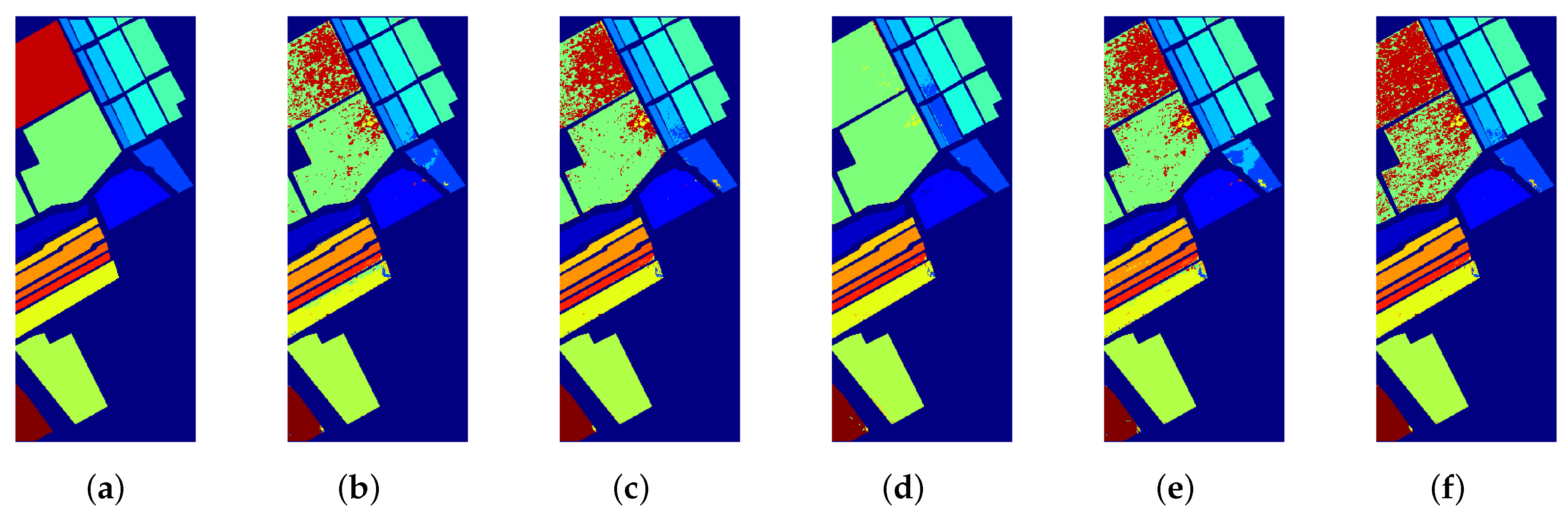
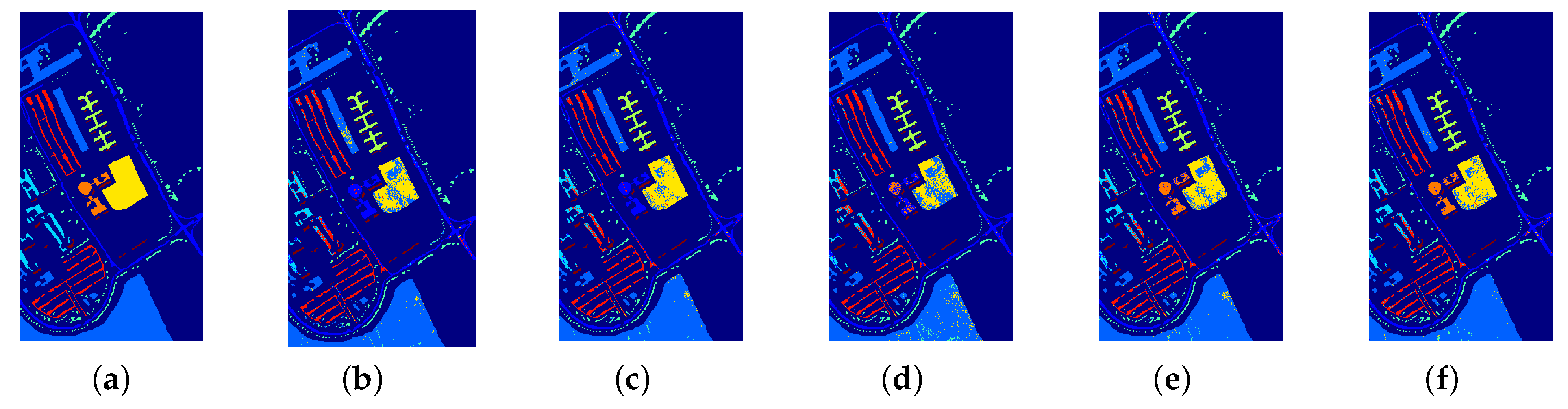
We conduct comparison experiments on the Salinas dataset and Pavia University dataset, respectively. The four comparison algorithms are Random Selection (RS), Breaking Ties (BT) [18], Margin Sampling (MS) [10], and Least Confident (LC) [24]. These algorithms all use the same initial samples, number of samples per generation, and the number of iterations as JPPAL_CRF. Figure 2 and Figure 3 represent the visual classification maps of the five experiments on Salinas and Pavia University, respectively. LC tends to select samples whose maximum posterior probability is closest to 0.5. However, it loses the information implied by the rest of the label distribution. The samples selected by BT are likely to be trapped in a single-category boundary. The overall accuracy of MS is poor, which varies widely for different classes. As a result, these algorithms show many misclassification results. It can be seen that our method (see Figure 2f and Figure 3f) shows results closer to the ground-truth image (see Figure 2a and Figure 3a) than other methods (see Figure 2b–d and Figure 3b–d).

Table 2. Classification results of the RS, BT, MS, LC, and JPPAL_CRF on the Salinas dataset (%), and the best result is bolded.

Class	RS	BT	MS	LC	JPPAL_CRF
1	96.12 (1.45)	99.84 (0.27)	99.08 (1.78)	99.94 (0.09)	99.60 (0.61)
2	99.21 (0.44)	99.39 (0.29)	99.76 (0.12)	97.68 (1.92)	99.87 (0.19)
3	86.58 (8.08)	91.13 (3.40)	83.29 (14.10)	74.65 (10.74)	98.48 (1.38)
4	99.47 (0.23)	97.29 (0.47)	99.06 (0.17)	96.75 (0.84)	96.93 (0.78)
5	95.93 (1.84)	97.86 (2.70)	99.23 (0.24)	89.77 (10.21)	98.83 (0.41)
6	99.71 (0.05)	99.87 (0.09)	99.98 (0.02)	99.62 (0.49)	99.98 (0.02)
7	99.32 (0.09)	99.79 (0.18)	99.99 (0.02)	99.44 (0.36)	99.92 (0.04)
8	90.71 (1.09)	83.57 (3.71)	64.85 (5.00)	92.10 (9.61)	90.16 (4.12)
9	97.77 (1.33)	98.58 (0.31)	99.59 (0.08)	94.92 (5.60)	99.98 (0.04)
10	88.15 (1.26)	88.87 (2.05)	95.88 (2.30)	77.40 (11.80)	94.52 (0.93)
11	88.13 (5.33)	89.16 (1.43)	94.02 (4.13)	83.60 (25.18)	97.34 (0.67)
12	99.50 (0.65)	97.19 (0.25)	99.01 (0.38)	92.35 (7.79)	100.00 (0.00)
13	97.94 (0.53)	96.04 (1.60)	98.09 (1.12)	96.70 (3.49)	96.11 (1.25)
14	92.11 (0.55)	95.90 (1.14)	97.17 (1.22)	98.30 (1.63)	97.87 (1.47)
15	46.70 (3.16)	71.62 (9.18)	65.14 (18.85)	91.03 (10.30)	71.32 (12.46)
16	94.03 (4.29)	99.14 (0.30)	99.76 (0.19)	99.61 (0.22)	98.76 (0.27)
OA	88.32 (0.39)	90.29 (1.08)	85.96 (1.97)	87.77 (1.40)	93.34 (0.85)
AA	91.96 (0.55)	94.08 (0.43)	93.37 (1.10)	91.90 (2.00)	96.23 (0.54)
Kappa	86.95 (0.44)	89.21 (1.18)	84.26 (2.25)	86.36 (1.55)	92.58 (0.97)

and

Table 3. Classification results of the RS, BT, MS, LC, and JPPAL_CRF on the Pavia University dataset (%), and the best result is bolded.

Class	RS	BT	MS	LC	JPPAL_CRF
1	90.02 (3.07)	92.68 (2.13)	86.92 (2.95)	92.41 (1.28)	97.86 (0.37)
2	98.23 (0.58)	93.33 (1.57)	88.72 (2.25)	93.20 (2.18)	99.31 (0.42)
3	57.12 (7.75)	83.55 (4.29)	89.99 (1.77)	82.00 (3.17)	78.88 (6.39)
4	87.88 (1.64)	97.12 (0.39)	91.84 (3.49)	96.18 (0.83)	93.99 (2.66)
5	98.94 (0.28)	99.61 (0.32)	99.88 (0.11)	99.88 (0.59)	99.76 (0.20)
6	63.89 (2.05)	92.22 (1.90)	59.92 (13.55)	92.68 (2.63)	91.90 (0.98)
7	48.15 (11.70)	86.16 (5.78)	79.53 (12.56)	81.10 (9.36)	86.05 (6.49)
8	89.74 (2.03)	80.69 (1.61)	72.66 (2.80)	79.94 (2.64)	95.11 (1.64)
9	99.79 (0.14)	99.96 (0.08)	99.96 (0.08)	99.96 (0.08)	99.32 (0.31)
OA	87.93 (0.48)	91.80 (0.48)	82.44 (2.99)	91.31 (0.72)	96.07 (0.65)
AA	81.53 (1.17)	91.70 (0.77)	85.49 (2.13)	90.71 (1.02)	93.58 (1.64)
Kappa	83.66 (0.63)	89.02 (0.67)	76.89 (3.65)	88.36 (1.02)	94.76 (0.88)

give the classification results of the five algorithms on Salinas and Pavia University. The results show that the values of JPPAL_CRF are always the highest on OA, AA, and Kappa. The relatively low OAs of all the comparison algorithms suggest that these algorithms are more extreme in the sample selection. JPPAL_CRF mitigates the effect of the first two maximum posterior probabilities while the remaining posterior probabilities are incorporated. It allows more valuable samples to be selected during active learning. In the classification stage, CRF is used to mine spatial domain information so that some error-prone classification categories have higher accuracy. Our method improves overall classification accuracy and maintains a balance of all feature classes. Thus, JPPAL_CRF outperforms other methods from the perspective of classification accuracy.

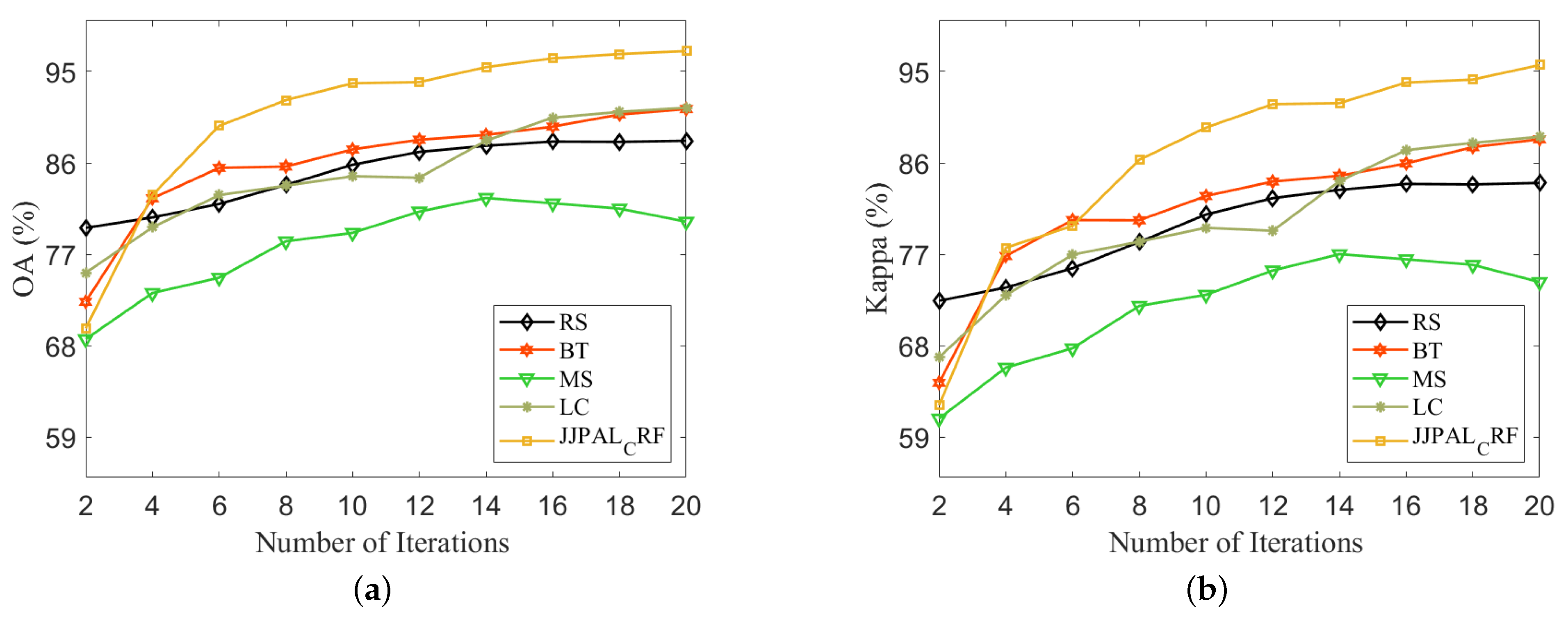
Figure 4 shows the OA and Kappa of each method on the Salinas dataset with respect to the number of iterations. It can be seen that JPPAL_CRF always has a high increase in performance as the number of iterations increases. However, the OA and Kappa of other comparison methods converge quickly. This suggests that it is difficult for these methods to select more valuable samples after a certain number of samples are selected actively. Figure 5 shows the OA and Kappa of each method on the Pavia University dataset with respect to the number of iterations. Although the performance of JPPAL_CRF is low when the training samples are small, it increases rapidly as the number of iterations increases. This suggests that JPPAL_CRF still has greater potential for selecting valuable samples as the number of times increases.

4. Conclusions

In this paper, we propose a JPPAL_CRF, whose basic idea is to make full use of all the information in the posterior probability matrix while selecting labeled samples. It incorporates all posterior probabilities into the decision function. Compared with other approaches, this approach can select samples that are more conducive to classification during the sampling process because of the extended variability between samples. For further improving the classification effect and alleviating the phenomenon of “same objects with different spectrums” and “different objects with the same spectrum”, this paper uses CRF. CRF takes into account spatial domain information and label constraints. It retains detailed information about each class and post-processes the classification results to further improve classification results. The experiments on two common datasets show that the proposed approach possesses significant performance advantages. In the future, we will extend the combination of active learning and CRF by adding random field potentials to the active-learning decision function.

References

- Huang, Y.; Zhou, X.; Xi, B.; Li, J.; Kang, J.; Tang, S.; Chen, Z.; Hong, W. Diverse-Region Hyperspectral Image Classification via Superpixelwise Graph Convolution Technique. Remote Sens. 2022, 14, 2659–2670. [Google Scholar]
- Li, Q.; Yuan, Y.; Jia, X.; Wang, Q. Dual-stage approach toward hyperspectral image super-resolution. IEEE Trans. Image Process. 2022, 31, 7252–7263. [Google Scholar] [CrossRef]
- Meng, Z.; Li, L.; Jiao, L.; Liang, M. Fully dense multiscale fusion network for hyperspectral image classification. Remote Sens. 2019, 11, 2718. [Google Scholar] [CrossRef] [Green Version]
- Yang, J.; Zhao, Y.-Q.; Chan, J.C.-W. Learning and transferring deep joint spectral-spatial features for hyperspectral classification. IEEE Trans. Geosci. Remote Sens. 2017, 55, 4729–4742. [Google Scholar] [CrossRef]
- Li, Q.; Gong, M.; Yuan, Y.; Wang, Q. Symmetrical feature propagation network for hyperspectral image super-resolution. IEEE Trans. Geosci. Remote Sens. 2022, 60, 1–12. [Google Scholar] [CrossRef]
- Zhang, Z.; Pasolli, E.; Crawford, M.M. An adaptive multiview active learning approach for spectral–spatial classification of hyperspectral images. IEEE Trans. Geosci. Remote Sens. 2020, 58, 2557–2570. [Google Scholar] [CrossRef]
- Li, J.; Bioucas-Dias, J.M.; Plaza, A. Hyperspectral image segmentation using a new bayesian approach with active learning. IEEE Trans. Geosci. Remote Sens. 2011, 49, 3947–3960. [Google Scholar] [CrossRef] [Green Version]
- Crawford, M.M.; Tuia, D.; Yang, H.L. Active learning: Any value for classification of remotely sensed data? Proc. IEEE 2013, 101, 593–608. [Google Scholar] [CrossRef] [Green Version]
- Li, Y.; Lu, T.; Li, S. Subpixel-pixel-superpixel-based multiview active learning for hyperspectral images classification. IEEE Trans. Geosci. Remote Sens. 2020, 58, 4976–4988. [Google Scholar] [CrossRef]
- Tuia, D.; Ratle, F.; Pacifici, F.; Kanevski, M.F.; Emery, W.J. Active learning methods for remote sensing image classification. IEEE Trans. Geosci. Remote Sens. 2009, 47, 2218–2232. [Google Scholar] [CrossRef]
- Tuia, D.; Volpi, M.; Copa, L.; Kanevski, M.; Munoz-Mari, J. A survey of active learning algorithms for supervised remote sensing image classification. IEEE J. Sel. Topics Signal Process. 2011, 5, 606–617. [Google Scholar] [CrossRef]
- Xu, X.; Li, J.; Li, S. Multiview intensity-based active learning for hyperspectral image classification. IEEE Trans. Geosci. Remote Sens. 2018, 56, 669–680. [Google Scholar] [CrossRef]
- Xu, M.; Zhao, Q.; Jia, S. Multiview spatial–spectral active learning for hyperspectral image classification. IEEE Trans. Geosci. Remote Sens. 2022, 60, 1–15. [Google Scholar] [CrossRef]
- Zhou, X.; Prasad, S.; Crawford, M.M. Wavelet-domain multiview active learning for spatial-spectral hyperspectral image classification. IEEE J. Sel. Top. Appl. Earth Observ. Remote Sens. 2016, 9, 4047–4059. [Google Scholar] [CrossRef]
- Copa, L.; Tuia, D.; Volpi, M.; Kaneski, M. Unbiased query-by-bagging active learning for VHR image classification. In Proceedings of the SPIE-The International Society for Optical Engineering, Liptovský Ján, Slovakia, 6–10 September 2010; pp. 78300K-1–78300K-8. [Google Scholar]
- Mitra, P.; Shankar, B.U.; Pal, S.K. Segmentation of multispectral remote sensing images using active support vector machines. Pattern Recognit. Lett. 2004, 25, 1067–1074. [Google Scholar] [CrossRef]
- Luo, T.; Kramer, K.; Goldgof, D.B.; Samson, A.R.S.; Hopkins, T.; Cohn, D. Active learning to recognize multiple types of plankton. J. Mach. Learn Res. 2005, 6, 589–613. [Google Scholar]
- Sun, S.; Zhong, P.; Xiao, H.; Wang, R. An MRF model-based active learning framework for the spectral-spatial classification of hyperspectral imagery. IEEE J. Sel. Top. Signal Process. 2015, 9, 1074–1088. [Google Scholar] [CrossRef]
- Zhong, P.; Wang, R. Learning conditional random fields for classification of hyperspectral images. IEEE Trans. Image Process. 2010, 19, 1890–1907. [Google Scholar] [CrossRef]
- Zhang, G.Y.; Jia, X.P. Simplified conditional random fields with class boundary constraint for spectral–spatial based remote sensing image classification. IEEE Geosci. Remote Sens. Lett. 2012, 9, 856–860. [Google Scholar] [CrossRef]
- Shotton, J.; Winn, J.; Rother, C.; Criminisi, A. Textonboost: Joint appearance, shape and context modeling for multi-class object recognition and segmentation. Proc. Euro. Conf. Comput. Vis. 2006, 9, 1–15. [Google Scholar]
- Zhong, Y.; Lin, X.; Zhang, L. A support vector conditional random fields classifier with a mahalanobis distance boundary constraint for high spatial resolution remote sensing imagery. IEEE J. Sel. Top. Appl. Earth Observ. Remote Sens. 2014, 7, 1314–1330. [Google Scholar] [CrossRef]
- Li, J.; Bioucas-Dias, J.M.; Plaza, A. Spectral-spatial classifica- tion of hyperspectral data using loopy belief propagation and active learning. IEEE Trans. Geosci. Remote Sens. 2013, 51, 844–856. [Google Scholar] [CrossRef]
- Settles, B. Active Learning Literature Survey; University of Wisconsin: Madison, WI, USA, 2009; Volume 1648. [Google Scholar]
Figure 1.
Overall framework of JPPAL_CRF using AL to select the most valuable samples to expand the labeled set, and then using CRF to optimize the classification results.
Figure 2.
The visual comparison results of classification maps in Salinas. (a) Ground-truth image. (b) RS. (c) BT. (d) MS. (e) LC. (f) JPPAL_CRF.
Figure 3.
The visual comparison results of classification maps on Pavia University. (a) Ground-truth image. (b) RS. (c) BT. (d) MS. (e) LC. (f) JPPAL_CRF.
Figure 4.
Classification results for each comparison experiment on the Salinas dataset. (a) OA. (b) Kappa.
Figure 5.
Classification results for each comparison experiment on the Pavia University dataset. (a) OA. (b) Kappa.