
E-FPN: Evidential Feature Pyramid Network for Ship Classification


1
College of Information Engineering, Shanghai Maritime University, Shanghai 201306, China
2
College of Logistics Engineering, Shanghai Maritime University, Shanghai 201306, China
3
Jiangsu Automation Research Institute, Lianyungang 222061, China
*
Author to whom correspondence should be addressed.
Remote Sens. 2023, 15(15), 3916; https://doi.org/10.3390/rs15153916
Submission received: 12 June 2023
/
Revised: 3 August 2023
/
Accepted: 3 August 2023
/
Published: 7 August 2023
(This article belongs to the Section AI Remote Sensing)
Abstract
:Ship classification, as an important problem in the field of computer vision, has been the focus of research for various algorithms over the past few decades. In particular, convolutional neural networks (CNNs) have become one of the most popular models for ship classification tasks, especially using deep learning methods. Currently, several classical methods have used single-scale features to tackle ship classification, without paying much attention to the impact of multiscale features. Therefore, this paper proposes a multiscale feature fusion ship classification method based on evidence theory. In this method, multiple scales of features were utilized to fuse the feature maps of three different sizes (40 × 40 × 256, 20 × 20 × 512, and 10 × 10 × 1024), which were used to perform ship classification tasks separately. Finally, the multiscales-based classification results were treated as pieces of evidence and fused at the decision level using evidence theory to obtain the final classification result. Experimental results demonstrate that, compared to classical classification networks, this method can effectively improve classification accuracy.
1. Introduction
Image classification, as an important problem in the field of computer vision, aims to assign input images to predefined categories. Over the past few decades, significant progress has been made in image classification, especially with respect to deep-learning-based methods. CNNs can automatically extract rich feature representations from input images and perform classification using fully connected layers. Compared to traditional machine learning methods, deep learning approaches can learn more discriminative features automatically from data, thereby leading to higher classification accuracy. The practical applications of image classification techniques have become relatively mature and have been widely used in various domains, such as visual recognition [1], medical image analysis [2], industrial quality inspection [3], agriculture [4,5,6], surveillance [7], and autonomous driving [8].
However, due to the complex and diverse characteristics of image data and the variety of practical application scenarios, improving the accuracy of image classification further remains a challenging task. For instance, challenges persist in satellite remote-sensing image classification [9,10,11,12], as well as fine-grained image classification [13,14].
For example, ship satellite remote sensing images present specific challenges compared to traditional natural images in the image classification task: [15,16,17].
- 1.
- Variations in ship size and shape: The appearance and shape of ships in satellite remote sensing images can be influenced by various factors such as distance, lighting conditions, and viewing angles. Therefore, ships of the same type may exhibit different sizes and shapes in different satellite remote-sensing images, thereby making image classification difficult.
- 2.
- Complexity of the background: Ship satellite remote-sensing images often include complex backgrounds such as waves, clouds, and ports. These backgrounds can introduce interference in the classification of ships.
- 3.
- Similarity: Ship satellite remote-sensing images encompass various types of ships, including different ship types that include cargo ships, passenger ships, and fishing boats. However, apart from some specific ship types, most ship outlines exhibit an elongated shape with axis symmetry and a pointed bow, which can pose challenges for classification algorithms.
- 4.
- Resolution: Ship satellite remote-sensing images typically have lower resolutions compared to traditional natural images. This can impact the extraction of fine-grained ship details and features, thus affecting the performance of classification algorithms.
- 5.
- Data quality: Ship satellite remote-sensing images are susceptible to natural factors such as lighting, weather conditions, and cloud cover, which can result in lower image quality. Issues such as blurring, distortion, and occlusion can arise, thereby affecting the accuracy of ship classification.
Currently, most existing improvement methods for ship classification, which rely on CNNs to automatically extract abstract features, mainly focus on modifying network structures, optimizing training strategies, or redesigning loss functions in an iterative manner. However, they overlook the further processing of the classification results.
In the case of fine-grained image classification, which is different from general ship classification tasks, the main challenge lies in categorizing objects from closely related subcategories. These objects often exhibit subtle category differences, and the crucial information containing these differences is typically localized in small regions of the image. When extracting features using deep neural networks, smaller-sized features in the images may become diluted as the network deepens, thereby affecting the classification results [18]. Utilizing multiscale feature fusion methods allows deep networks to learn small-sized features that may have been diluted due to network depth, thereby enhancing the accuracy of classification. Therefore, solely focusing on network structure or loss function improvements may pose challenges in further enhancing the classification performance.
In the CNN-based methods, initially, researchers focused on deepening the network structure to improve the classification performance and to address issues arising from deeper networks in order to enhance the classification network. Later, the attention shifted toward better feature propagation or utilizing detailed features to strengthen the classification performance. For example, attention mechanisms were introduced to emphasize more discriminative features [19], or multiple feature extraction networks were used in combination with extracted feature maps to complement missing features [20]. Knowledge distillation was also employed to transfer detailed image features to smaller primary networks, thus resulting in improved performance for the classification network [21]. However, the above approaches added additional complexity to the network structures in order to better extract features.
This paper proposes a multiscale ship classification network that applies evidence theory to decision-level fusion to break free from the improvement loop mentioned earlier and to enhance the classification accuracy from a different perspective. Three main modules were utilized in this method to ensure better classification accuracy: (1) a multiscale output module of the feature extraction network; (2) a pyramid feature fusion module; and (3) a decision-level fusion module based on evidence theory. The first two parts focused on improving accuracy using network structures, while the final part emphasized optimizing classification performance using the final probability distribution information.
To validate the feasibility of this method, experiments were conducted on a traditional natural image dataset and a remote-sensing image dataset for fine-grained ship classification. Several comparisons were made with classical classification methods. The experimental results demonstrate that the proposed method—E-FPN—achieved better classification accuracy and consistency compared to classical classification methods. The main contributions of this paper are as follows:
- 1.
- To address the issue of information loss during the feature extraction process, feature-level fusion was performed by selecting feature maps of different depths from the backbone feature extraction network. This fusion aimed to supplement the lost information.
- 2.
- The classification results from multiple scales were further fused at the decision level using fusion rules based on evidence theory. The different classification results were treated as pieces of evidence, and the differences in the probability distributions were utilized to optimize the classification results.
The remaining sections of this paper are composed as follows. Section 2 provides a review of related works. Section 3 introduces the relevant background knowledge. Section 4 presents the overall network structure of the E-FPN. Section 5 provides detailed explanations of the experimental setup, including parameter settings, experimental procedures, and parameter discussions. Finally, in Section 6, the paper concludes with a summary and discusses future research directions.
2. Related Work
At the algorithmic level, deep-learning-based image classification methods can be divided into two categories based on different feature extractors. The first category is CNN-based image classification methods, which have achieved remarkable breakthroughs in the past decade based on modern deep learning techniques. Krizhevsky et al. introduced rectified linear units (ReLU) in convolutional neural networks to achieve nonlinearity and used the Dropout technique to mitigate overfitting and learn more complex objects [22]. Karen Simonyan and Andrew Zisserman improved upon AlexNet by stacking 3 × 3 convolutions and deepening the network structure to enhance the classification accuracy [23]. However, as the networks became deeper, issues such as network degradation, vanishing gradients, and exploding gradients emerged. To address these problems, Kaiming He et al. introduced Batch Normalization (BN) to replace Dropout and solve the issues of vanishing and exploding gradients. They also introduced residual connections to address network degradation [24]. SainingXie et al. introduced Inception on top of ResNet, thereby transforming single-path convolutions into multi-path convolutions with multiple branches [25]. Gao Huang et al. proposed DenseNet in 2017, which connects each layer with all previous layers in a feed-forward fashion to alleviate the vanishing gradient problem and enhance feature propagation [26]. Tsung-Yu Lin et al. used two feature extractors to extract features from input images and combined them using a bilinear pooling function before performing classification to compensate for the features lost by a single feature extractor (B-CNN) [27]. To fully exploit the small features that can differentiate different categories, Jianlong Fu et al. proposed RA-CNN, which focuses the classification operation on regions with differentiating features using a recurrent attention projection mechanism [28].
To enhance the classification accuracy of CNN-based classification networks for satellite remote-sensing images, Linqing Huang et al. proposed a classification method that converts images in the dataset into different color spaces and trains separate CNNs on each color space. Finally, the output results of each classifier were fused using evidence theory [29]. Yue Chen et al. presented a method called Destruction and Construction Learning (DCL), which disrupts and shuffles input images to emphasize local detailed features. They employed a region alignment network to restore the image layout and learn semantic information from local regions, thereby strengthening the connections between neighboring regions [30]. Heliang Zheng et al. introduced a technique that extracts precise attention maps to highlight target regions with rich detailed features at a high resolution. They also employed knowledge distillation to transfer image detail features to the main network for image classification [31].
The second approach is based on the visual transformer method [32]. Similar to CNNs, transformers have dominated the field of natural language processing (NLP) in the past decade. Initially, when transformers were introduced to computer vision, they were primarily used to extract global contextual information from images, but their performance outcomes were not satisfactory. In the past two years, there have been breakthroughs in using large-scale pretraining on transformer-based CNN classification networks, which have surpassed the dominance of CNNs in traditional image domains. Examples of such networks include the Vision Transformer (ViT) [33] and Shifted Window Transformer (SWIN-Transformer) [34].
In recent years, advancements in ship classification algorithms have involved various improvement approaches in academic research. For instance, Chen et al. employed a contrastive learning method to replace classical classification techniques. They designed a loss function to separate different categories and bring together similar ones [35]. Zhang et al. adopted a combination of traditional feature extraction methods and modern abstract feature extraction methods to enhance the representation capability of ship features [18]. Guo et al. utilized shape-aware feature extraction techniques, thereby allowing the feature extraction process to better align with the distinctive spindle-shaped appearance of ships [36]. Building upon the bilinear pooling method, Zhang et al. made improvements to make it more suitable for ship classification tasks [37]. Additionally, Jahan et al. employed knowledge distillation and class balancing methods to achieve ship classification in SAR ship images [38].
3. Preliminaries
3.1. Cross-Stage Partial Darknet (CSPDarkNet)
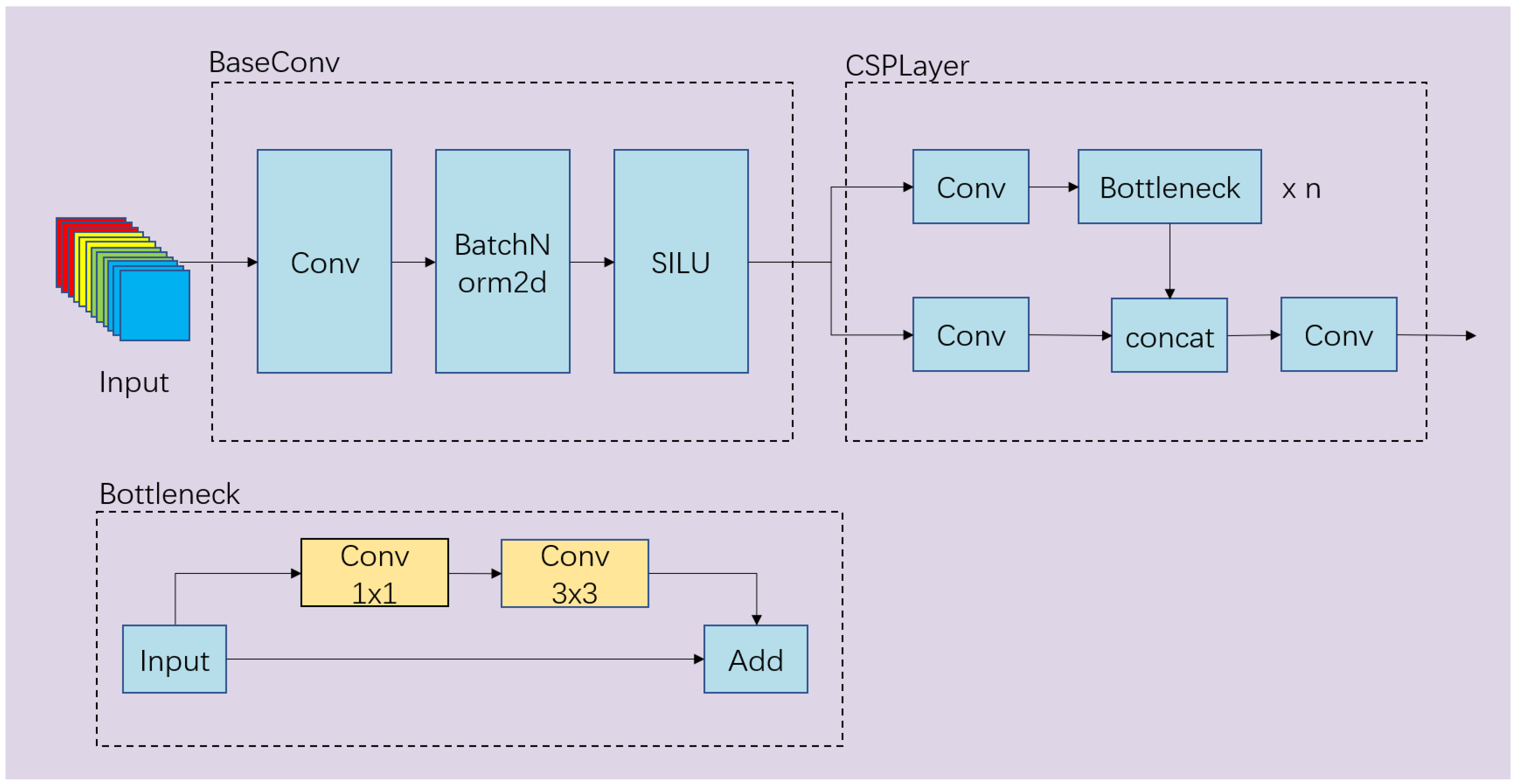
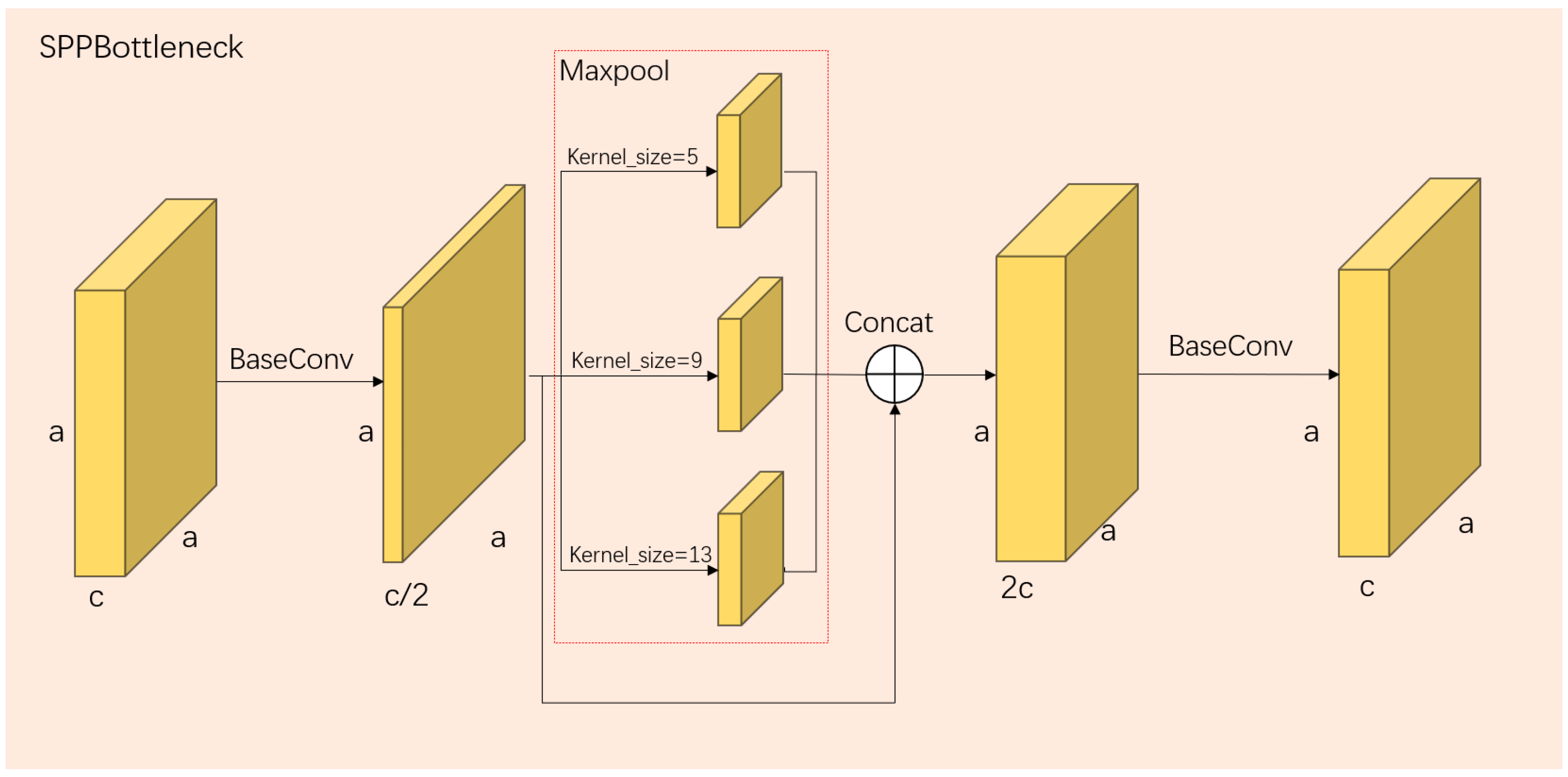
CSPDarkNet [39] can be divided into five main parts: Focus, Dark2, Dark3, Dark4, and Dark5, in sequential order. The Focus module focuses on aggregating the width and height information of the image into the channel information by subsampling the image’s pixel values. The structures of Dark2 to Dark4 are well demonstrated in Figure 1, where each Dark part consists of a BaseConv layer and a CSPLayer. Each BaseConv layer consists of a convolutional layer, a BatchNorm2d layer, and an activation function. The entire CSPLayer can be viewed as a residual module, where one side of the residual branch passes through the BaseConv layer once, while the other side goes through n bottleneck units after the BaseConv layer. The two parts are then concatenated and subjected to another BaseConv operation. The structure of the bottleneck unit, as shown in Figure 1, involves a 1 × 1 and a 3 × 3 convolution for the main branch, while the residual branch remains unchanged, and the two parts are finally added together. The Dark5 part is slightly different from the previous three parts. It introduces a Spatial Pyramid Pooling (SPP-Bottleneck) module between the BaseConv and CSPLayer, which utilizes max pooling with three different kernel sizes to extract features, and it then combines them to increase the network’s receptive field. Its structure is depicted in Figure 2.
3.2. Feature Pyramid Networks (FPNs)
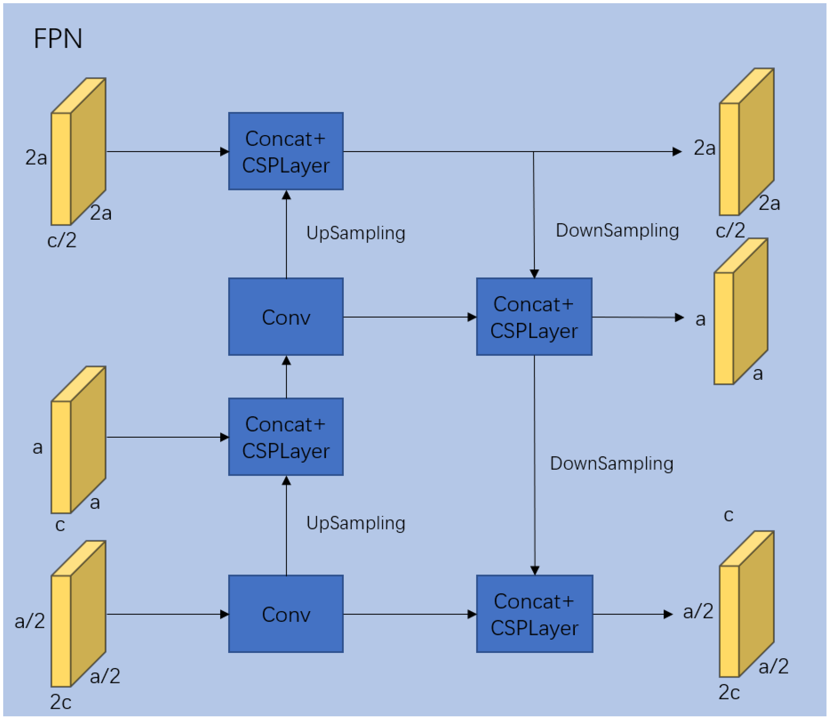
In convolutional networks, deep layers are more responsive to semantic features, while shallow layers are more responsive to image details. In image classification tasks, it has been validated by Karen Simonyan and others that deeper networks have a positive impact on image classification. However, deep convolutional layers tend to lose fine-grained details. Therefore, the FPN [40] model can be used to fuse features from shallow and deep layers, thereby allowing the deep layers to complement the information lost during multiple convolutional operations, which is beneficial for subsequent classification tasks. The FPN structure is illustrated in Figure 3.
3.3. Evidence Theory
The evidence theory, established by Dempster and Shafer, represents propositions using mathematical sets [41]. Unlike probability theory, which considers only single elements, evidence theory allows for multiple elements within a set. This theory is characterized by its ambiguity and the ability to perform imprecise reasoning at different levels of abstraction. It can differentiate between ignorance and equiprobability, thereby enabling a better representation of uncertain propositions. Evidence theory simulates the normal human thinking process, where one observes and collects information before synthesizing it from various aspects to make judgments and obtain results for a given problem.
In the Dempster–Shafer (DS) evidence theory, the sample space composed of all propositions is defined as a discernment framework, which is denoted as . It is a set comprising a group of mutually exclusive and collectively exhaustive propositions representing all the possible answers to a given question. Let us assume another discernment framework defined as , where represents a set of basic hypotheses, and are subsets of that set. The power set of is the set of all its subsets and is denoted as .
Basic probability assignment (BPA) refers to the process of calculating the basic probabilities for each piece of evidence in the discernment framework . This process is accomplished using the basic probability assignment function, which is denoted as the mass function m(x), which reflects the degree of belief or confidence in a proposition. The mass function satisfies the following properties:
In evidence theory, the uncertainty of evidence can be quantified using the belief function Bel(A) and the plausibility function Pl(A). The definitions and the relationship between the belief and plausibility functions are as follows:
where K represents the conflict coefficient, which can describe the magnitude of conflict between items of evidence—a higher value of K indicates a greater degree of conflict between the evidence. serves as a normalization factor. For the combination of multiple items of evidence, the calculation follows a similar approach. Multiple belief functions can be combined using an orthogonal sum to generate a new mass function, which is denoted as . If this combination exists, the order of calculation does not affect the result, thus satisfying the commutative and associative properties.
Suppose that there are n sets of evidence , with their corresponding basic belief assignment functions , respectively, and focal elements , respectively, within the given recognition framework. The classical Dempster’s combination rule for these sets can be defined as follows:
The classical Dempster’s combination rule is susceptible to paradoxes [42], and there are several classic paradoxical situations:
- 1.
- Conflict of evidence: When the basic belief assignment functions of multiple evidence sources exhibit strong conflicts, the fusion process may lead to highly unreasonable results and even fail to generate a consistent synthesis (known as a complete conflict, i.e., K = 1).
- 2.
- One-vote veto: If there is a piece of evidence for which the basic belief assignment function for a specific proposition is 0, the fusion result will be 0, regardless of the values of the other evidence’s belief assignment functions. This reflects the limitation of the DS fusion rule with regard to allocating conflict properly. For example, assume that there is evidence E1: m1(a) = 0.999, m1(b) = 0.001, m1(c) = 0; E2: m2(a) = 0, m2(b) = 0.001, and m2(c) = 0.999. Using the formula, we calculate the results as m(a) = m(c) = 0, and m(b) = 1. Clearly, the results are unreasonable.
- 3.
- Poor robustness: Although the changes in the basic belief assignment values of the focal elements in the evidence are minimal, the synthesized results can be completely different. For example, modifying the evidence E1 in the previous example results in: m1(a) = 0.998, m1(b) = 0.001, and m1(c) = 0.001; however, the synthesized result shows that m(b) = 0.001, which is contrary to the previous result.
The Dezert–Smarandache Theory (DSmT) has made improvements to address the aforementioned issues. One of these improvements is the Proportional Conflict Redistribution Rule No. 5 (PCR5) [43], which reduces the generation of unreasonable results caused by significant conflicts between the items of evidence compared to the DS fusion method. Additionally, weights can be assigned to the outputs of the FPN before performing the fusion operation to mitigate conflicts. In the PCR5 fusion rule, the conflicting degrees are proportionally allocated to each focal element, thereby enabling a more reasonable fusion of two sources of evidence with high conflicts. The fusion method of the PCR5 is described as follows:
Among them, and represent the two items of evidence; A and B denote the focal elements contained in the evidence; represents the nonconflicting product, and the latter part of the sum represents the allocation of all the conflicting products containing A on A.
The weighting calculation method used in the experiment referred to the approach proposed by Zhunga Liu et al. [44], which adds a weight to the prefused data by calculating the difference between two BPAs. The mass values corresponding to the two classifiers indicate the likelihood of the corresponding class being true, with higher values suggesting a higher probability. The collection of all the classes that are judged as true can be represented as follows:
Among them, represents the set of true classes. denotes a threshold set between 0 and 1. When the ratio of the mass value corresponding to a class of the maximum mass value in that BPA exceeds the threshold, it is considered that the class may also be true. This approach increases the tolerance for differences between the two classification results while retaining information that is beneficial for the final classification result. The calculation method for the difference between the two BPAs is as follows:
The weight can be represented as follows:
The weights are used to discount the two BPAs using Shafer’s discounting operation, thus aiming to reduce conflicts between the two classifiers:
By employing the operation of adding weights, it is possible to reduce the negative impact of the classifier with lower classification ability on the final fusion results when there is significant conflict between the two classifiers. This, in turn, enhances the accuracy of the ultimate fusion outcome.
4. Methodolgy
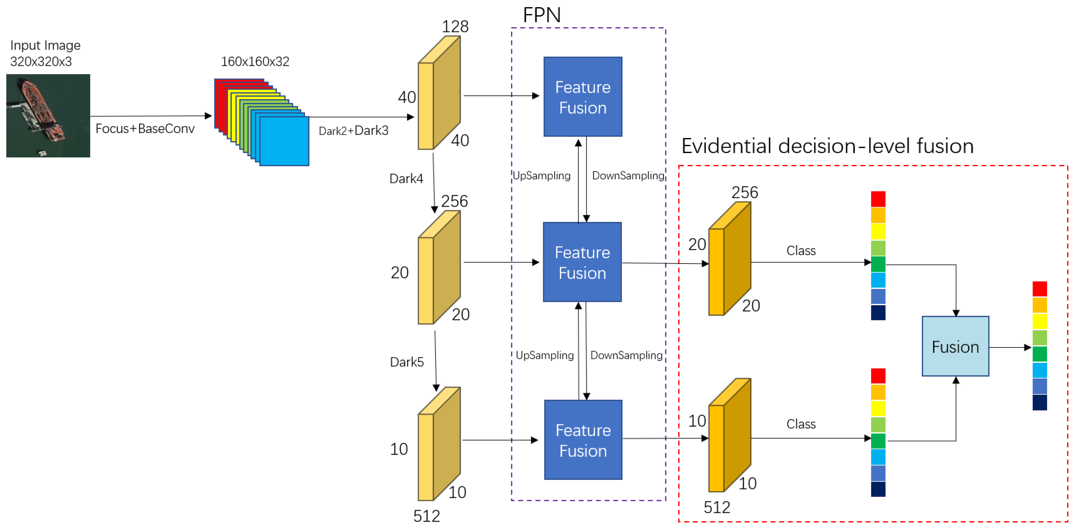
Most existing CNN-based models only utilize features or scales from the final stage as the ultimate classification features, thereby making them single-scale classification models. However, the shallow-level features of the network contain more detailed information. Neglecting shallow-level features without considering them can lead to decreased classification accuracy for similar or small objects during the classification process. Particularly when the image resolution is low, shallow-level features can retain more information and reduce the risk of feature loss. To better utilize the features of shallow-level networks, this paper proposes a method that uses multiscale features and employs the feature pyramid network (FPN) to fuse features from different scales. The fusion of multiple classification results is achieved using the fusion rules of evidence theory. This approach enables the model to learn abstract features at different levels of abstraction on different scales, thereby improving the model’s classification accuracy and enhancing decision-making capabilities. Consequently, the E-FPN consists of three main components: the feature extraction network, the FPN feature fusion part, and the decision-level fusion based on evidence theory. Specifically, the feature extraction part is responsible for extracting abstract features from the images, the FPN feature fusion part combines features from different scales, and the decision-level fusion part, based on evidence theory, integrates the classification results from multiple scales into the final classification result. Figure 4 illustrates the overall network structure of the proposed method in this paper. The feature extraction part utilizes the backbone network structure of YOLOX, which usies Darknet53 as the main network for extracting image features. Darknet53 combines the characteristics of ResNet and uses a residual network to ensure that the gradient problem caused by excessively deep networks is avoided during feature representation. From Figure 4, it can be observed that the Dark3, Dark4, and Dark5 parts of the Darknet53 feature the extraction network output feature maps of three different dimensionalities. These feature maps contain features of the objects to be classified at three different scales, and all three scales of feature maps are involved in the final classification decision step. In other words, by utilizing feature maps from different depths of the network for multiscale feature fusion, better feature representation capability is ensured. For this feature extraction network, the chosen image input size was set to 320 × 320. As the network layers increased, the input image dimension transitioned from 320 × 320 to 40 × 40 for Dark3, 20 × 20 for Dark4, and 10 × 10 for Dark5. Considering the depth of the feature extraction network, choosing larger or smaller image input sizes would result in insufficient feature extraction or feature loss, which is not conducive to classification decision making. In fact, selecting an appropriate input size is also consistent with mature CNN models, such as VGG and ResNet.
By extracting the features at different stages of the feature extraction network, different scales of feature maps are obtained, thereby capturing information at three different scales. However, directly performing classification operations on these feature maps is not sufficient. Although the shallow-level feature information can propagate to deeper layers in the network, it may become diluted during convolutional operations, thereby leading to the neglect of detailed information in the resulting deep-level features and a decrease in classification accuracy. From Figure 4, it can be observed that feature maps from different stages or scales participate in the object classification task. Therefore, the classification results obtained from the feature maps at different scales will affect the final classification accuracy. It is necessary to enhance the classification accuracy of the feature maps at different scales involved in the classification task as much as possible. To address this issue, this paper introduces a multiscale feature fusion method. This method allows the deep-level network to learn detailed feature information from the shallow-level network, while the shallow-level network can learn abstract feature information from the deep-level network, thus improving the feature representation capability. With this approach, each scale of the feature map can learn richer information, thereby leading to better classification accuracy in the subsequent classification process and ultimately improving the final classification accuracy. Subsequent experiments demonstrate that using the multiscale feature fusion methods can improve the accuracy of object classification. It achieves better classification results compared to using single-scale feature-based classification methods.
In light of the above, this paper employed a feature pyramid network (FPN) to perform feature-level fusion of the three feature maps obtained from the backbone network, thereby aiming to complement the diluted detailed features during the feature extraction process. By obtaining three feature maps with the same input dimensions, classification operations were separately performed on two of the feature maps, thereby resulting in two sets of classification results. In this paper, evidence theory was used to fuse the classification results from different scales. Evidence theory can handle uncertainty and incomplete information by combining multiple pieces of evidence to improve classification accuracy. The multiscale output classification results are treated as distinct sources of evidence, which are fused at the decision level using evidence theory to obtain the final classification result. Specifically, the classification results obtained from the feature maps of different scales can be regarded as different sources of evidence, and the obtained classification results can be seen as probability distributions, where each element represents the probability value of a corresponding class. Therefore, the maximum probability value in the obtained probability distribution cannot solely represent the current target class, as other higher probability values may correspond to the correct class as well. Hence, the obtained multiple probability distributions can serve as references from different aspects, rather than being definitive classification results. The use of evidence theory enables the integration of the probability distributions obtained from different scales as different pieces of evidence, and through analyzing the differences between these pieces of evidence, a new probability distribution is derived as the classification result. This classification method resembles the decision-making process of human experts, who analyze and study information from multiple sources to make an informed judgment, thus resulting in a relatively accurate answer. Subsequent experiments have demonstrated that fusing the multiscale classification results using evidence theory can further improve the accuracy of ship classification, thereby validating the effectiveness and applicability of the evidence theory in ship classification.
In this paper, the input images to the network were set to a size of 320 × 320 in order to retain detailed features in the images. Various image augmentation techniques, such as random horizontal flipping, occlusion, and cropping, were applied to augment the dataset and enhance the network’s performance. The input network used was CSPDarkNet, where the images were processed through the Focus module to extract a value for every other pixel, thus resulting in four feature maps that were then combined together. This process reduces the width and height information of the image while increasing the number of channels. This reduces the number of parameters and improves the network’s performance while minimizing the loss of original information.
Among them, the input image X undergoes a slicing operation, which is denoted as X[], where every pixel value is extracted to obtain four feature maps. The concatenation operation concat() is then applied to combine these four feature maps. After the focus operation, the size of the resulting feature maps becomes 160 × 160 × 12.
After the Focus module, the feature extraction stage follows, which consists of Dark2–Dark5. The Dark5 part includes the SPP-Bottleneck module, which applies pooling layers with different kernel sizes to the image to increase the network’s receptive field and extract more features. In this study, the SPP-Bottleneck module utilized pooling kernels of sizes 5 × 5, 9 × 9, and 13 × 13. The feature maps obtained from Dark3–Dark5, denoted as I3–I5, were chosen as the outputs of the feature extraction network. The sizes of these feature maps were 40 × 40 × 256, 20 × 20 × 512, and 10 × 10 × 1024, respectively. Subsequently, these three feature maps were fed into the FPN network for feature-level fusion. In the fusion stage, the FPN layer took the three feature maps with different dimensions and performed upsampling and downsampling operations to integrate the features from multiple scales, thus enriching the information within the feature maps at different scales.
In the provided formulas, represents a convolutional operation applied to the feature map, while indicates the process of upsampling the feature map, followed by fusion with a shallow-level feature map and then downsampling. Finally, the resulting feature map is concatenated with the feature map processed through the operations to obtain the final feature map used for classification. During the upsampling and downsampling process, the combined feature map is further integrated using the CSPLayer. This results in three feature maps (I3–I5) with the same dimensions as the input. Among these, the feature maps corresponding to the Dark4 and Dark5 dimensions (I4 and I5, respectively) are selected for the classification process. The classification component consists of a BaseConv, two convolutional layers, and three linear layers. In the linear layers, the flattened feature maps are sequentially reduced to the dimensions of 256, 64, and 10, where the parameter 10 represents the number of classes for classification. The activation function is applied to obtain the probability distributions (m1 and m2) for the output feature maps corresponding to the Dark4 and Dark5 scales, respectively. These probability distributions from the two scales are considered as evidence sources for decision-level fusion.
where represents the i-th value, and C represents the number of outputs, which is the number of classes.
Although the feature maps between different dimensions complement each other with feature information through the FPN operation, the probability distribution results obtained from different-sized feature maps still exhibit variations after classification. Hence, the differences in information between these two probability distributions can be utilized to optimize the classification results. Treating these two probability distributions as two sources of evidence, whic are denoted as m1 and m2, the DS fusion rule is employed to merge them. Initially, the conflict coefficient K, which represents the degree of dissimilarity between the two pieces of evidence, is computed using Equation (7) based on m1 and m2. Subsequently, Equation (6) is applied to fuse the probability values of each class in m1 and m2, thereby resulting in a unique classification result. During the fusion process, the probability values corresponding to classes with relatively higher degrees of credibility in the probability distribution are accentuated, while the probability values corresponding to other classes are attenuated. If a scenario arises where two probability values in the distribution are similar, indicating hesitation between two classes, this method can leverage the differential information from other probability distributions to make decisions, thereby enhancing the reliability of the final classification result. Consequently, the final classification result is obtained. This approach provides a more reliable classification outcome compared to the individual fused results. The pseudocode for the E-FPN is presented in Algorithm 1.
In this case, and represent the outputs of each stage in the backbone network, and represent different parts of the backbone network, refers to the feature fusion operation, and K represents the conflict coefficient between the evidence. denotes the operation of flattening the feature map, represents the classification operation, and maps the obtained classification results to the range [0,1].
| Algorithm 1 The Method Processing of a Image |
| Input: A ship image X |
| begin |
| Do abstract feature extraction |
| End |
| Do FPN feature fusion |
| End |
| Do Classification |
| End |
| Do Decision fusion |
| End |
| Output: Classification tensor result |
5. Experimental
5.1. Dataset
In this section, to validate the effectiveness of the E-FPN and compare it with other image classification algorithms, two datasets, CIFAR-10 and FGSCR10, were used.
CIFAR-10 is a small-scale dataset used for general object recognition. It consists of 10 classes of RGB images, with 6000 images per class. The dataset was divided into a training set of 50,000 images and a test set of 10,000 images. The images have a size of 32 × 32 pixels. This dataset was used to evaluate the classification performance for traditional natural images.
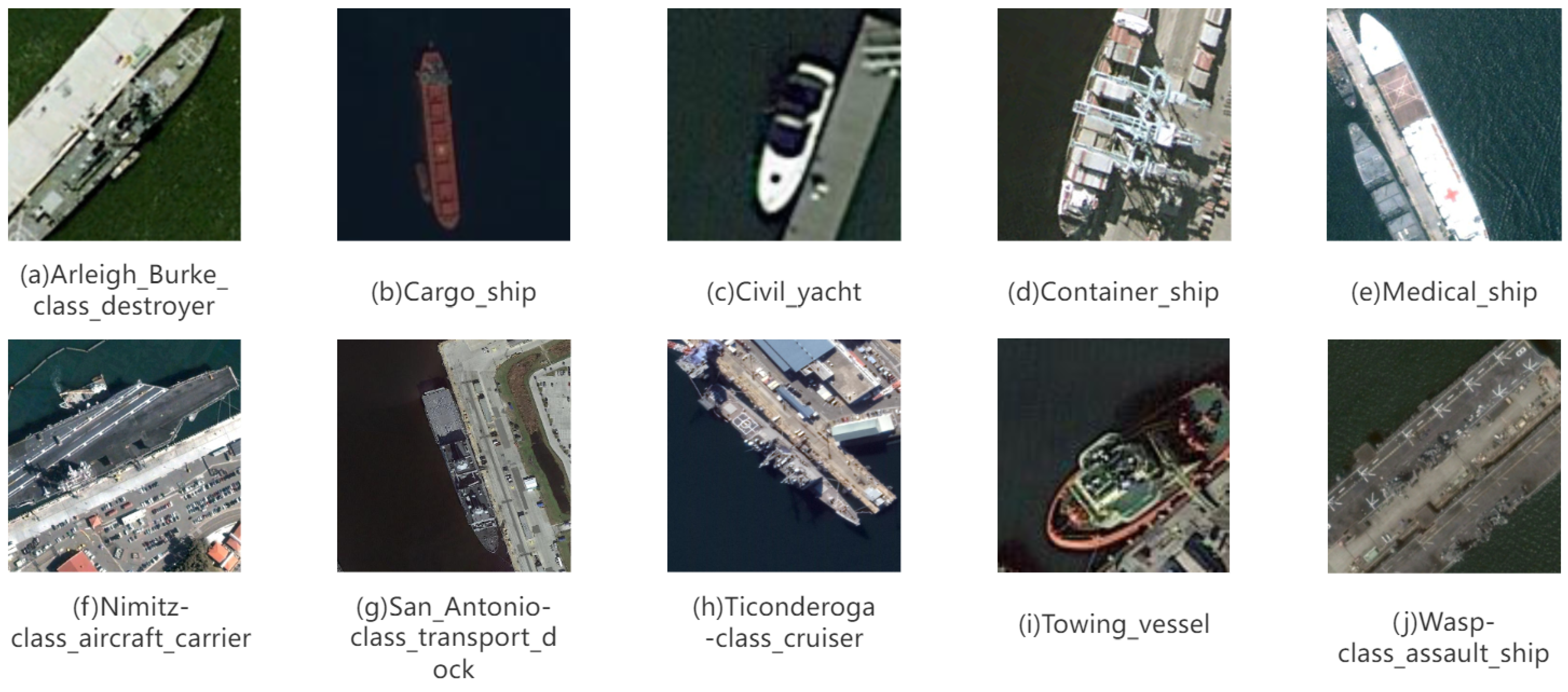
The FGSCR-42 dataset is a publicly available dataset for fine-grained ship classification in remote sensing images. It contains 42 classes with a total of 9320 images, and the images have varying resolutions. For the experiments in this section, we selected 10 classes with a larger number of image samples, thus resulting in a total of 5220 images. This dataset was used to evaluate the classification performance in the context of remote-sensing images and fine-grained object classification. The composition and sample images are shown in Table 1 and Figure 5, respectively.
5.2. Experimental Parameter Settings
In this study, we compared classic classification algorithms, namely ResNet50, ResNeXt50, VGG19, and VGG16, along with the fine-grained image classification algorithms B-CNN and DCL, against the E-FPN to evaluate its effectiveness. For the classic classification algorithms, the image size was uniformly adjusted to 224 × 224. Data augmentation techniques, including random horizontal flipping, random occlusion, and random cropping, were applied to the dataset images. The initial learning rate was set to 0.0001, and the training batch size, weight decay, and decay epoch were set to 64, 0.1, and 50, respectively. The Adam optimizer was selected, and the cross entropy loss function was employed for calculating the loss. In the proposed method, to preserve more image feature information, the dataset images were uniformly resized to 320 × 320 while keeping the remaining parameters consistent with the aforementioned settings. This was done to evaluate the effectiveness of the E-FPN in terms of classification performance by comparing it with the baseline models. Further details regarding the metrics and evaluation will be presented in the following sections. The experiments were conducted using the GPU resource A5000-24G.
5.3. Evaluation Indices
In this experiment, the overall accuracy (OA) and the Kappa statistic were employed as evaluation metrics to assess the classification performance of the models. The details are as follows:
- 1.
- OA: Overall accuracy is defined as the ratio of correctly classified samples to the total number of samples. The calculation method is as follows:where N represents the total number of image samples in the dataset. represents whether the classification of the ith sample is correct. If the classification is correct, the value of is 1; otherwise, it is 0.
- 2.
- The Kappa coefficient is used for consistency testing and can also be used to measure classification accuracy. Its calculation is based on the confusion matrix. The calculation method is as follows:where represents the ratio of the sum of correctly classified samples in each class to the total number of samples, which corresponds to the overall accuracy. Assuming that the true number of samples in each class is denoted as , the predicted number of samples in each class is denoted as , respectively, and the total number of samples is n, then the equation can be expressed as follows:
The calculation result of Kappa falls between [−1:1], but it typically ranges between [0:1]. It can be categorized into five levels to represent different levels of agreement: [0.0:0.20] indicates slight agreement, [0.21:0.40] indicates fair agreement, [0.41:0.60] indicates moderate agreement, [0.61:0.80] indicates substantial agreement, and [0.81:1] indicates almost perfect agreement.
5.4. Performance Evaluation
In this section, the effectiveness of the proposed method is evaluated by comparing it with classical image classification networks on the CIFAR-10 and FGSCR-10 datasets. The validation results are shown in Table 2 and Table 3. The bold typeface represents the best results, while underlining represents the second-best results.
In Table 2 and Table 3, two metrics were used to evaluate the classification performance, as well as to compare the four classical classification networks and two fine-grained image classification networks with the E-FPN. The proposed method was evaluated on the CIFAR-10 dataset using two metrics—OA and Kappa. The results indicate that the E-FPN achieved excellent performance in both metrics, with an OA of 94.78% and a Kappa value of 0.945, thereby obtaining the second-best and best scores, respectively. This demonstrates the effectiveness of the E-FPN with respect to the traditional natural image dataset.
In the FGSCR-10 dataset, the proposed method achieved an OA of 98.04% and a Kappa value of 0.9776. Compared to the other four classical methods, the E-FPN showed an improvement in the OA that ranged from 1.15% to 3.95% and an improvement in the Kappa metric that ranged from 0.0095 to 0.044. When compared with the other two fine-grained image classification algorithms, the E-FPN also achieved excellent results with the highest OA and Kappa values.
Through the experiments on the two datasets, it can be observed that all algorithms showed similar performance on the CIFAR-10 dataset, and in some cases, the B-CNN even exhibited lower accuracy compared to the baseline model. This could be attributed to the low resolution of the images in this dataset, as certain algorithmic improvements may not perform as effectively under such conditions.
In the FGSCR-10 dataset, the performance of the proposed method surpassed that of the other four baseline models. This may be due to the fact that the FGSCR-10 dataset involves fine-grained classification targets. After feature extraction by the backbone network, the E-FPN utilizes the FPN method to fuse features at different scales, which allows for complementary details among the three-dimensional feature maps. Finally, the classification results of the different feature maps are fused using the evidence-theory-based decision-level fusion method, thus further correcting the classification results. For example, when an image is misclassified, its correct classification has a probability value that is close to the probability value of the current misclassification. When another set of probability distributions is fused, the probability value corresponding to the correct classification is also large. After fusion, the probability value of the correct classification may become the largest, thus resulting in the final correct result. As a result, the proposed method demonstrates an advantage over the other methods in the FGSCR-10 dataset. Compared to the other two fine-grained image classification algorithms, our proposed E-FPN outperformed the B-CNN and DCL. This may be attributed to the effective extraction of the objects’ fine-grained features using our multiscale approach, and the decision-level fusion enables a comprehensive analysis of the classification results from different perspectives.
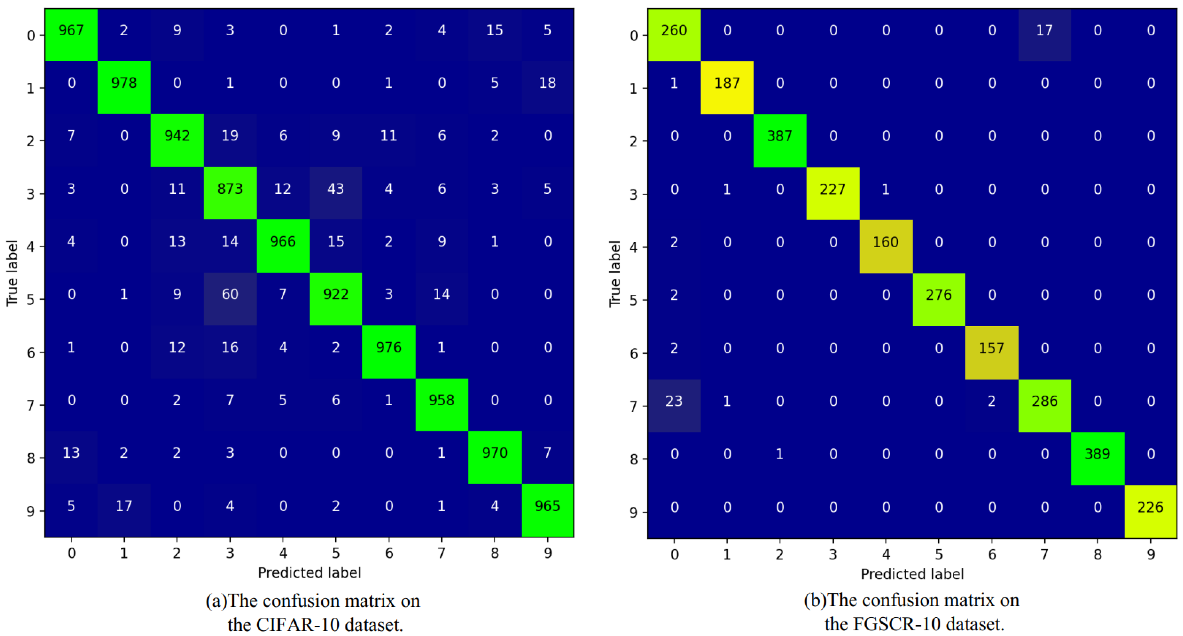
In terms of the Kappa metric, all classification methods achieved a performance exceeding 90% on both datasets, thus indicating a level of consistency that is considered “almost perfect”. Compared to the other four baseline models, the E-FPN exhibited further improvement in this metric, thus signifying enhanced classification accuracy for each class and its general applicability. Additionally, when compared to the fine-grained image recognition algorithms (B-CNN and DCL), the E-FPN also showed improvement in terms of the Kappa value. Furthermore, Figure 6 provides a detailed visualization of the classification results for each class, which demonstrates the proposed method’s performance in terms of confusion matrices for both the CIFAR-10 and FGSCR-10 datasets. There are very few dark areas outside of the diagonal, thus indicating a reduced number of misclassifications. This visual representation intuitively demonstrates the effectiveness of the E-FPN.
Table 4 presents the number of parameters, FLOPs (floating-point operations), and inference times for the seven models. It can be observed that the VGG16 and VGG19 had significantly higher numbers of parameters and FLOPs compared to the other baseline models. This is likely due to their deeper network architectures and the utilization of numerous convolutional layers. On the other hand, the ResNet50 and ResNeXt50 had smaller numbers of parameters and FLOPs. This reduction can be attributed to the utilization of residual structures, which help reduce network depth and complexity. Among the five methods, the E-FPN had a higher number of parameters compared to the ResNet50 and ResNeXt50, but it was lower than the VGG16 and VGG19. However, its FLOPs were the lowest among the five methods, thus indicating a relatively low computational cost when performing the classification task. This is because the proposed method introduces an additional FPN network, while the backbone network adopts the residual approach to reduce its depth. When comparing the fine-grained image classification models, the E-FPN had the highest number of parameters, thus suggesting higher storage requirements. However, its FLOPs remained the lowest, which indicates that, compared to the other six models, the E-FPN requires fewer computational resources during the inference phase, thereby making it suitable for deployment on mobile and edge devices. This observation is evident from the inference speed, where all three fine-grained image recognition models, including the E-FPN, required higher inference times than the four baseline models. However, in the fine-grained image recognition models, the inference time of the E-FPN model was lower than the other two (B-CNN and DCL). This demonstrates the advantage of the E-FPN in terms of the inference speed.
Additionally, the DS fusion method used in the E-FPN incurred minimal additional computational costs for the network. As a result, the increase in network parameters was relatively small, and the FLOPs were the lowest among the all models.
By comparing the experimental results from the two aforementioned tables, it can be concluded that the E-FPN is effective with respect to both traditional natural image datasets and fine-grained remote sensing image datasets. In the description of the FPN network structure, it was mentioned that three feature maps of different dimensions were utilized, but during the final decision-level fusion, only the results from the deeper two scales of the feature maps were selected for fusion. In the following, we will discuss the impact of choosing different dimension feature maps for decision-level fusion on the final results. The results of these experiments are presented in Table 5 and Table 6.
In this experiment, different combinations of feature maps were fused for each dataset, and the impact of the pairwise fusion of different feature maps on the final results was compared. The last line represents the results obtained by fusing all three feature maps together. Dark3–Dark5 represent the probability distributions of the classification results from the FPN fused outputs of the backbone network. In Table 5, the CIFAR-10 dataset was used. It can be observed that, before decision-level fusion, the OA gradually improved as the network layers deepened. However, after fusion, the OA was lower than the OA of the Dark5 output result. Among the fused results, the fusion of Dark4 and Dark5 achieved the highest OA of 94.92%. Furthermore, its Kappa value was superior to the other three results, which came out to 0.945. Preliminary analysis suggests that this may be due to significant conflicts in the probability values among certain categories before fusion, thereby resulting in an unreasonable probability distribution after fusion, thus leading to incorrect fusion results. Further investigation of this issue will be discussed in subsequent sections.
Table 6 displays the results obtained from the FGSCR-10 dataset: Dark3–Dark5 had the same classification OA of 97.73%. However, the OA improved after fusion. The fusion of the Dark3 and Dark4 achieved an OA of 97.8%, while the fusions of the Dark4 and Dark5, Dark3 and Dark5, and all three (Dark3–Dark5) had an OA of 98.04%. The performance of the Kappa index was consistent with the OA, with the fusion of the Dark3 and Dark4 resulting in a Kappa value of 0.975, while the other three fusions all had Kappa values of 0.978. By comparing the results before and after fusion, it can be observed that the samples correctly classified by the Dark3–Dark5 were not entirely the same, and, in the probability distributions of misclassified samples, the probability values for the correct class were close to those of the misclassified class. Therefore, after fusion, some misclassified samples were corrected, thereby resulting in an improvement in the final OA of the results.
According to the above table, it can be observed that the highest OA resulted after fusions were obtained by combining Dark5 with other parts, and these results were superior to the results obtained by fusing the Dark3 and Dark4. It can be seen that the results obtained from the deeper parts of the network had a more reliable probability distribution. However, the results obtained by fusing all three parts together showed a slight decrease compared to the fusion of the Dark4 and Dark5. This may be due to the fact that, during fusion, the probability values of the correct class and the misclassified class for all three inputs were very close, and since the Dark3 had classification errors, the final result was not corrected to the correct class during fusion, thereby resulting in a decrease in the OA. Therefore, in the experiment, this study chose to fuse the Dark4 and Dark5 for the fusion process.
The E-FPN in this paper consists of three parts: the feature extraction network, the FPN network, and the decision fusion part. During the training process, the crossentropy loss values of the three outputs from the FPN were summed to calculate the overall loss value. Specifically, the obtained loss values in the network are referred to as loss_0, loss_1, and loss_2. However, for the final decision, only the output results from the Dark4 and Dark5 were selected for fusion. Therefore, the next step was to explore the impact of the loss_0 value obtained from Dark2 on the classification performance and the effect of using the FPN for fusion at the feature level.
According to the experimental results in Table 7, for the CIFAR-10 dataset, the removal of the loss_0 slightly improved the OA to 95.13%. This may be because the FPN has multiple output classification results, and adding the loss_0 during the training process may have led to oscillation and decision risk. Additionally, the OA gap between the Dark4 and Dark5 was very small, and their Kappa values were similar. Without using the FPN for feature-level fusion, the OA was lower in both cases, and the fused OA and Kappa values were also lower compared to the two cases with theFPN. This indicates that the classification results of the shallow layers may have had a negative impact on the decision-making and fusion in the datasets with clear image features. However, the positive impact of the shallow layers in the feature-level fusion should not be ignored, as shown in Table 8.
When conducting experiments on the FGSCR-10 dataset, it was found that adding the loss_0 and using the FPN for feature-level fusion resulted in a higher OA and Kappa values compared to not using the FPN or not adding the loss_0, wherein 98.04% and 0.978 were achieved, respectively. This indicates that the classification performance for each class object in the dataset was excellent. Under the conditions of removing the FPN and removing the loss_0, the OA gap between the Dark4, Dark5, and the fused result was small. However, it can be observed that the OA of the fused result was better than the individual results. As mentioned earlier, although the outputs of the shallow network can have a negative impact on the final decision-level fusion, the features learned by the shallow network still have a positive influence on the classification results in the feature-level fusion process.
Based on the experiments and discussions, it can be concluded that using the FPN structure and training the shallow network for classification improved the classification performance on the fine-grained remote-sensing image dataset. The FPN structure complemented the detailed features that were lost in the deep network. Since the FPN structure used in the paper involved the fusion of the information from the three layers, adding the loss_0 for classification training in the top layer of the network could facilitate the learning of more useful feature information, thereby further enhancing the feature fusion effect. The results in Table 8 indicate that employing the feature-level fusion method helped improve the classification performance of fine-grained remote-sensing image classification and further enhanced the classification performance after decision-level fusion.
The experimental parameter section in this paper mentions that, unlike the four other classification methods used in the comparative experiments, the image input size for the E-FPN in this paper was 320 × 320, while the four classical classification methods used an image input size of 224 × 224. The purpose of this choice was to preserve more image feature information. However, it should be noted that a larger input image size does not necessarily guarantee better performance. Table 9 and Table 10 present a comparison of the impact of different input image sizes on the classification performance.
In the experiments comparing the impact of different input image sizes on the classification performance, the image size of 224 × 224, which is the same as the other four classical algorithms, was selected. Additionally, scaled versions of the 640 × 640 and 160 × 160 were used. Based on the data in Table 9 and Table 10, it was found that the input image size of 320 × 320 achieved the best performance in terms of the classification OA and Kappa value. Furthermore, in both tables, as the input image size decreased from large to small, the classification the OA initially increased and then decreased. Therefore, it is not necessarily true that a larger input image size leads to better performance, and the appropriate size should be chosen based on the specific circumstances.
Table 9 presents the influence of different input image sizes on classification performance, which reveals that the classification OA for each size increased with the depth of the network. Except for the 320 × 320 size group, all other size groups exhibited an increase in the classification OA after decision-level fusion. However, the final accuracy remained lower than that of the 320 × 320 size group. Regarding the Kappa index, the 320 × 320 size group still performed the best. These data indicate that, for traditional natural image datasets, which have easily discernible image features, adequate feature extraction enabled effective classification, thereby only necessitating the selection of an appropriate input image size.
Table 10 demonstrates the impact of different input image sizes on the classification performance in the FGSCR-10 dataset. In contrast to Table 9, Table 10 does not observe an increase in the classification OA with the network depth. In the 640 × 640 and 160 × 160 size groups, a decline in the classification OA was observed as the network depth increased. This may have been due to excessively large or small feature maps that failed to effectively propagate relevant features in the FPN feature fusion. For the 160 × 160 size group, the small image size may have led to the loss of crucial detail features, thereby resulting in a reduced classification OA. This could also result in significant conflicts between the generated probability distributions, thereby making it difficult to correct misclassifications during the decision-level fusion and ultimately decreasing the OA of the fused results. In the 320 × 320 size group, the Dark3–Dark5 exhibited a higher classification OA than the other groups. Although these three groups had the same classification accuracy, the decision-level fusion further enhances their OA values. These data demonstrate that the proposed classification method, when applied to fine-grained remote sensing image datasets, benefits from using appropriately sized input images. This enabled the extraction of abstract features while retaining some detailed features, thereby facilitating subsequent image classification operations.
In the previous sections, we discussed the network architecture and input image data. In Section 2, the limitations of the DS fusion method were mentioned; specifically, the issue of unreasonable fusion results when significant conflicts exist between two input evidence factors were discussed. To overcome this problem, this paper adopted the PCR5 fusion method and utilized the Shafer discounting method to weigh the evidence, thereby reducing the conflicts between input evidence. The obtained results were compared with those of the DS fusion method.
Table 11 and Table 12 present the OA and Kappa values obtained using three different fusion rules for the CIFAR-10 dataset. The DS fusion rule was the fusion rule adopted in this paper, the PCR5 was the proportional conflict redistribution method mentioned in Section 2 of this paper, and wPCR5 refers to the addition of weights to the probability distributions before using the PCR5 fusion rule by applying the Shafer discounting method to discount the evidence and reduce conflicts between input data. From Table 11, it can be observed that the OA values of the Dark3 × Dark4, Dark3 × Dark5, and Dark4 × Dark5 combinations under the DS fusion rule and PCR5 fusion rule were almost indistinguishable. However, for the Dark4 × Dark5 combination, the OA decreased when using the PCR5 rule compared to using the DS rule. After applying the wPCR5 fusion rule, the OA improved compared to both the DS rule and the PCR5 rule for all three combinations. This improvement may have been attributed to the already high classification OA before fusion, thereby indicating a relatively small conflict between the probability distributions of the two input data. The PCR5 fusion rule primarily aims to mitigate the impact of the conflicts on the fusion results and to prevent the generation of unreasonable output values. By adding weights and employing the PCR5 rule, the conflicts between the two inputs can be further effectively reduced, thereby leading to better results. The Kappa values generally exhibited a similar pattern to the OA results. The wPCR5 rule yielded slightly better results compared to the DS and PCR5 rules, but the improvement was marginal, while there was little difference between the DS rule and the PCR5 rule.
Table 13 and Table 14 compare the OA and Kappa values for the FGSCR-10 dataset. Similar to the results obtained on the CIFAR-10 dataset, the DS fusion rule and the PCR5 fusion rule yielded nearly identical results. However, for the Dark3 × Dark5 combination with higher conflicts, the PCR5 rule slightly outperformed the DS rule. When using the wPCR5 rule, the performance was slightly worse than when using the previous two rules. The same trend was observed in the Kappa values. However, in the case of the fine-grained remote-sensing image datasets, the probability values of each class in the classification distributions were close, thereby making it difficult to compute favorable weights, as was mentioned in Section 2. Consequently, the weighting approach weakened the confidence of certain correctly classified classes during the discounting operations, thereby resulting in suboptimal final results. Regarding the Kappa values, there was little difference among the three fusion methods.
Based on the above analysis, it can be observed that the DS fusion rule and the PCR5 fusion rule yielded almost identical results on both datasets. The wPCR5 method performed slightly better than the previous two methods with respect to the traditional natural image datasets but slightly worse with respect to the fine-grained remote-sensing image datasets. Additionally, the computation complexities of the PCR5 and wPCR5 were higher than that of the DS rule, and the complexities increased more noticeably with a larger number of classes to be classified. Therefore, when there was no significant conflict between the two probability distributions, the DS fusion rule was chosen in this paper.
In the previous experiments, it was mentioned that, in the fine-grained remote-sensing image dataset, the method of adding weights to reduce the conflicts between the evidence actually weakened the credibility of some correctly classified results. In the process of calculating the weights, a threshold was set for the ratio between the mass values of each class and the maximum mass value to preserve the differences between the two classification results.
In the previous experiments, a threshold of 0.5 was set. The impact of the threshold value on the OA and Kappa value after fusion can be seen in Table 15 and Table 16.
The above table demonstrates the influence of the threshold values ranging from 0.1 to 0.9 for the classification OA and consistency with respect to the two datasets. In the CIFAR-10 dataset, as the threshold value increased from 0.1 to 0.9, the classification OA gradually rose to 95.17%. Compared to the threshold value of 0.1, there was an improvement of 0.24%. The Kappa value increased from 0.9436 to 0.9463. In this dataset, when the threshold value increased, it filtered out categories with lower probability values in the probability distributions, thereby retaining other potential options for correct classification. This preserved some differences between the classifiers as complementary information, which benefitted subsequent fusion operations.
In the FGSCR-10 dataset, changing the threshold value from 0.1 to 0.9 had almost no impact on the classification OA and Kappa values. This indicates that the threshold value had little effect on the fusion results in this dataset. Table 17 displays the partial probability distributions generated by Dark5. It can be observed that the reason for this phenomenon is that one class in the probability distribution—before fusion—had a significantly high probability value, and the ratios of other probabilities to it were lower than 0.1. Consequently, the variation in the threshold value did not affect the final result.
Based on the experiments, it can be concluded that the threshold value has almost no impact on the classification of OA in the FGSCR-10 dataset. In the CIFAR-10 dataset used in this experiment, setting a higher threshold value allows for the rational utilization of the differences between different classifiers, thereby obtaining complementary information and improving the OA of the classification results.
6. Conclusions
This study proposed a feature fusion and decision fusion method that combined the FPN with evidence theory to improve the classification accuracy. The effectiveness of this method was validated on both traditional natural image datasets and fine-grained remote-sensing image classification datasets. For the fine-grained remote-sensing image dataset, the FPN was utilized for feature-level fusion to capture the lost detailed features in the shallow networks. Simultaneously, evidence theory was applied to modify the generated probability distributions. In the experimental section, the network architecture and the parameters of this method were discussed, and the impact of different fusion rules on the final classification accuracy was compared. The experimental results demonstrate that selecting appropriate sizes of input images and using both feature-level fusion and decision-level fusion can effectively improve the classification accuracy. Additionally, reducing the conflicts between different classifier results through the addition of weights contributes to the enhancement of the classification results in certain cases.
The proposed E-FPN method still has some issues that need to be optimized. For instance, as demonstrated in Table 2, Table 3 and Table 4 in Section 5.4 of the paper, the E-FPN did not achieve significant improvement compared to the other three fine-grained image classification algorithms in the ship fine-grained classification task. Furthermore, when compared to the baseline models for the CIFAR-10 dataset, the improvement of our proposed method was not significant. We believe this is due to the small-image resolution in this dataset, where the utilization of multiscale features might not effectively extract and fuse large-scale and small-scale features, thereby leading to the incomplete exploitation of the advantages of multiscale features. Additionally, the E-FPN has a higher number of parameters than other algorithms, which demand significant storage resources when deployed, and this limitation requires optimization in future work.
Moreover, the current usage of the E-FPN involves the classification of single, complete images, which poses significant challenges when encountering scenarios with multiple objects or complex background environments in the image.
Future work should focus on applying this method to different feature extraction networks and exploring its generalizability. Additionally, further research should explore detail-oriented feature extraction and fusion methods to replace the fusion of entire feature maps, thereby aiming to reduce the complexity and the number of parameters of the method. Simultaneously, it is important to explore methods that prioritize the object’s location in the image to mitigate the interference caused by the background objects in the classification process.
Author Contributions
Y.D. and K.X. proposed the core framework design idea of E-FPN network. Y.D., K.X. and C.Z. participated in conducting the code implementation, experimental analysis, and manuscript writing. E.G. and Y.L. provided valuable advice on the methodology and carefully modified the manuscript. All authors have read and agreed to the published version of the manuscript.
Funding
This work was supported in part by the National Natural Science Foundation of China under Grant 62103258; National Key Research and Development Program of China (No. 2021YFC2801001); Shanghai Pujiang Program (No.22PJD029); Shanghai Yangfan Program (21YF1416700).
Data Availability Statement
The FGSCR-42 dataset in this study is openly and freely available at https://github.com/DYH666/FGSCR-42 (accessed on 11 March 2023). The CIFAR-10 dataset in this study will be openly and freely available at https://www.cs.toronto.edu/~kriz/cifar.html (accessed on 20 May 2023).
Conflicts of Interest
The authors declare no conflict of interest.
References
- Mahaur, B.; Mishra, K.; Singh, N. Improved Residual Network based on norm-preservation for visual recognition. Neural Netw. 2023, 157, 305–322. [Google Scholar] [CrossRef]
- Hesamian, M.H.; Jia, W.; He, X.; Kennedy, P. Deep learning techniques for medical image segmentation: Achievements and challenges. J. Digit. Imaging 2019, 32, 582–596. [Google Scholar] [CrossRef] [PubMed] [Green Version]
- Sundaram, S.; Zeid, A. Artificial intelligence-based smart quality inspection for manufacturing. Micromachines 2023, 14, 570–589. [Google Scholar] [CrossRef] [PubMed]
- Azizah, L.M.; Umayah, S.F.; Riyadi, S.; Damarjati, C.; Utama, N.A. Deep learning implementation using convolutional neural network in mangosteen surface defect detection. In Proceedings of the 2017 7th IEEE International Conference on Control System, Computing and Engineering (ICCSCE), Penang, Malaysia, 24–26 November 2017; IEEE: Piscataway, NJ, USA, 2017; pp. 242–246. [Google Scholar]
- Kurihara, J.; Nagata, T.; Tomiyama, H. Rice Yield Prediction in Different Growth Environments Using Unmanned Aerial Vehicle-Based Hyperspectral Imaging. Remote Sens. 2023, 15, 2004–2022. [Google Scholar] [CrossRef]
- Liu, M.; Su, W.H.; Wang, X.Q. Quantitative Evaluation of Maize Emergence Using UAV Imagery and Deep Learning. Remote Sens. 2023, 15, 1979–1994. [Google Scholar] [CrossRef]
- Akcay, S.; Breckon, T. Towards automatic threat detection: A survey of advances of deep learning within X-ray security imaging. Pattern Recognit. 2022, 122, 108245–108266. [Google Scholar] [CrossRef]
- Xu, Y.; Wang, H.; Liu, X.; He, H.R.; Gu, Q.; Sun, W. Learning to see the hidden part of the vehicle in the autopilot scene. Electronics 2019, 8, 331–347. [Google Scholar] [CrossRef] [Green Version]
- Wang, G.; Chen, H.; Chen, L.; Zhuang, Y.; Zhang, S.; Zhang, T.; Dong, H.; Gao, P. P2FEViT: Plug-and-Play CNN Feature Embedded Hybrid Vision Transformer for Remote Sensing Image Classification. Remote Sens. 2023, 15, 1773–1799. [Google Scholar] [CrossRef]
- Li, W.; Chen, H.; Liu, Q.; Liu, H.; Wang, Y.; Gui, G. Attention mechanism and depthwise separable convolution aided 3DCNN for hyperspectral remote sensing image classification. Remote Sens. 2022, 14, 2215–2241. [Google Scholar] [CrossRef]
- Liang, L.; Zhang, S.; Li, J.; Plaza, A.; Cui, Z. Multi-Scale Spectral-Spatial Attention Network for Hyperspectral Image Classification Combining 2D Octave and 3D Convolutional Neural Networks. Remote Sens. 2023, 15, 1758–1782. [Google Scholar] [CrossRef]
- Shi, C.; Zhang, X.; Sun, J.; Wang, L. Remote sensing scene image classification based on self-compensating convolution neural network. Remote Sens. 2022, 14, 545–573. [Google Scholar] [CrossRef]
- Ke, X.; Cai, Y.; Chen, B.; Liu, H.; Guo, W. Granularity-Aware Distillation and Structure Modeling Region Proposal Network for Fine-Grained Image Classification. Pattern Recognit. 2023, 137, 109305–109319. [Google Scholar] [CrossRef]
- Zhao, P.; Li, Y.; Tang, B.; Liu, H.; Yao, S. Feature relocation network for fine-grained image classification. Neural Netw. 2023, 161, 306–317. [Google Scholar] [CrossRef]
- Chen, L.; Shi, W.; Deng, D. Improved YOLOv3 based on attention mechanism for fast and accurate ship detection in optical remote sensing images. Remote Sens. 2021, 13, 660. [Google Scholar] [CrossRef]
- Li, B.; Xie, X.; Wei, X.; Tang, W. Ship detection and classification from optical remote sensing images: A survey. Chin. J. Aeronaut. 2021, 34, 145–163. [Google Scholar] [CrossRef]
- Dong, Y.; Chen, F.; Han, S.; Liu, H. Ship object detection of remote sensing image based on visual attention. Remote Sens. 2021, 13, 3192. [Google Scholar] [CrossRef]
- Zhang, T.; Zhang, X.; Ke, X.; Liu, C.; Xu, X.; Zhan, X.; Wang, C.; Ahmad, I.; Zhou, Y.; Pan, D.; et al. HOG-ShipCLSNet: A novel deep learning network with hog feature fusion for SAR ship classification. IEEE Trans. Geosci. Remote Sens. 2021, 60, 5210322. [Google Scholar] [CrossRef]
- Xiong, W.; Xiong, Z.; Cui, Y. An explainable attention network for fine-grained ship classification using remote-sensing images. IEEE Trans. Geosci. Remote Sens. 2022, 60, 5620314. [Google Scholar] [CrossRef]
- Ouyang, L.; Fang, L.; Ji, X. Multigranularity Self-Attention Network for Fine-Grained Ship Detection in Remote Sensing Images. IEEE J. Sel. Top. Appl. Earth Obs. Remote Sens. 2022, 15, 9722–9732. [Google Scholar] [CrossRef]
- Jahan, C.S.; Savakis, A.; Blasch, E. Cross-modal knowledge distillation in deep networks for SAR image classification. In Proceedings of the Geospatial Informatics XII, Orlando, FL, USA, 3 April–12 June 2022; SPIE: Bellingham, WA, USA, 2022; Volume 12099, pp. 20–27. [Google Scholar]
- Krizhevsky, A.; Sutskever, I.; Hinton, G.E. Imagenet classification with deep convolutional neural networks. In Proceedings of the Advances in Neural Information Processing Systems 25 (NIPS 2012), Lake Tahoe, NV, USA, 3–6 December 2012; Volume 25. [Google Scholar]
- Simonyan, K.; Zisserman, A. Very deep convolutional networks for large-scale image recognition. arXiv 2014, arXiv:1409.1556. [Google Scholar]
- He, K.; Zhang, X.; Ren, S.; Sun, J. Deep residual learning for image recognition. In Proceedings of the IEEE Conference on Computer Vision and Pattern Recognition, Las Vegas, NV, USA, 26 June–1 July 2016; pp. 770–778. [Google Scholar]
- Xie, S.; Girshick, R.; Dollár, P.; Tu, Z.; He, K. Aggregated residual transformations for deep neural networks. In Proceedings of the IEEE Conference on Computer Vision and Pattern Recognition, Honolulu, HI, USA, 21–26 July 2017; pp. 1492–1500. [Google Scholar]
- Huang, G.; Liu, Z.; Van Der Maaten, L.; Weinberger, K.Q. Densely connected convolutional networks. In Proceedings of the IEEE Conference on Computer Vision and Pattern Recognition, Honolulu, HI, USA, 21–26 July 2017; pp. 4700–4708. [Google Scholar]
- Lin, T.Y.; RoyChowdhury, A.; Maji, S. Bilinear CNN models for fine-grained visual recognition. In Proceedings of the IEEE International Conference on Computer Vision, Santiago, Chile, 7–13 December 2015; pp. 1449–1457. [Google Scholar]
- Fu, J.; Zheng, H.; Mei, T. Look closer to see better: Recurrent attention convolutional neural network for fine-grained image recognition. In Proceedings of the IEEE Conference on Computer Vision and Pattern Recognition, Honolulu, HI, USA, 21–26 July 2017; pp. 4438–4446. [Google Scholar]
- Huang, L.; Zhao, W.; Liew, A.W.C.; You, Y. An evidential combination method with multi-color spaces for remote sensing image scene classification. Inf. Fusion 2023, 93, 209–226. [Google Scholar] [CrossRef]
- Chen, Y.; Bai, Y.; Zhang, W.; Mei, T. Destruction and construction learning for fine-grained image recognition. In Proceedings of the IEEE/CVF Conference on Computer Vision and Pattern Recognition, Long Beach, CA, USA, 15–20 June 2019; pp. 5157–5166. [Google Scholar]
- Zheng, H.; Fu, J.; Zha, Z.J.; Luo, J. Looking for the devil in the details: Learning trilinear attention sampling network for fine-grained image recognition. In Proceedings of the IEEE/CVF Conference on Computer Vision and Pattern Recognition, Long Beach, CA, USA, 15–20 June 2019; pp. 5012–5021. [Google Scholar]
- Chen, C.F.R.; Fan, Q.; Panda, R. Crossvit: Cross-attention multi-scale vision transformer for image classification. In Proceedings of the IEEE/CVF International Conference on Computer Vision, Montreal, BC, Canada, 11–17 October 2021; pp. 357–366. [Google Scholar]
- Dosovitskiy, A.; Beyer, L.; Kolesnikov, A.; Weissenborn, D.; Zhai, X.; Unterthiner, T.; Dehghani, M.; Minderer, M.; Heigold, G.; Gelly, S.; et al. An image is worth 16 × 16 words: Transformers for image recognition at scale. arXiv 2020, arXiv:2010.11929. [Google Scholar]
- Liu, Z.; Lin, Y.; Cao, Y.; Hu, H.; Wei, Y.; Zhang, Z.; Lin, S.; Guo, B. Swin transformer: Hierarchical vision transformer using shifted windows. In Proceedings of the IEEE/CVF International Conference on Computer Vision, Montreal, BC, Canada, 11–17 October 2021; pp. 10012–10022. [Google Scholar]
- Chen, J.; Chen, K.; Chen, H.; Li, W.; Zou, Z.; Shi, Z. Contrastive learning for fine-grained ship classification in remote sensing images. IEEE Trans. Geosci. Remote Sens. 2022, 60, 4707916. [Google Scholar] [CrossRef]
- Guo, B.; Zhang, R.; Guo, H.; Yang, W.; Yu, H.; Zhang, P.; Zou, T. Fine-Grained Ship Detection in High-Resolution Satellite Images With Shape-Aware Feature Learning. IEEE J. Sel. Top. Appl. Earth Obs. Remote Sens. 2023, 16, 1914–1926. [Google Scholar] [CrossRef]
- Zhang, Z.; Zhang, T.; Liu, Z.; Zhang, P.; Tu, S.; Li, Y.; Waqas, M. Fine-grained ship image recognition based on BCNN with inception and AM-Softmax. Comput. Mater. Contin. 2022, 73, 1527–1539. [Google Scholar]
- Jahan, C.S.; Savakis, A.; Blasch, E. Sar image classification with knowledge distillation and class balancing for long-tailed distributions. In Proceedings of the 2022 IEEE 14th Image, Video, and Multidimensional Signal Processing Workshop (IVMSP), Nafplio, Greece, 26–29 June 2022; IEEE: Piscataway, NJ, USA, 2022; pp. 1–5. [Google Scholar]
- Redmon, J.; Farhadi, A. Yolov3: An incremental improvement. arXiv 2018, arXiv:1804.02767. [Google Scholar]
- Lin, T.Y.; Dollár, P.; Girshick, R.; He, K.; Hariharan, B.; Belongie, S. Feature pyramid networks for object detection. In Proceedings of the IEEE Conference on Computer Vision and Pattern Recognition, Honolulu, HI, USA, 21–26 July 2017; pp. 2117–2125. [Google Scholar]
- Shafer, G. Dempster-shafer theory. Encycl. Artif. Intell. 1992, 1, 330–331. [Google Scholar]
- Lin, Y.; Li, Y.; Yin, X.; Dou, Z. Multisensor fault diagnosis modeling based on the evidence theory. IEEE Trans. Reliab. 2018, 67, 513–521. [Google Scholar] [CrossRef]
- Dezert, T.; Dezert, J.; Smarandache, F. Improvement of proportional conflict redistribution rules of combination of basic belief assignments. J. Adv. Inf. Fusion (JAIF) 2021, 16, 48–74. [Google Scholar]
- Liu, Z.; Pan, Q.; Dezert, J.; Han, J.W.; He, Y. Classifier fusion with contextual reliability evaluation. IEEE Trans. Cybern. 2017, 48, 1605–1618. [Google Scholar] [CrossRef]
Figure 1.
CSPDarkNet network structure.

Figure 2.
SPP-Bottleneck network structure.

Figure 3.
FPN network structure.

Figure 4.
E-FPN network structure.

Figure 5.
FGSCR-10 image examples.

Figure 6.
The confusion matrices of E-FPN on CIFAR-10 and FGSCR-10 are presented. (a) shows the confusion matrix obtained from the CIFAR-10 dataset, while (b) shows the confusion matrix obtained from the FGSCR-10 dataset.
Figure 6.
The confusion matrices of E-FPN on CIFAR-10 and FGSCR-10 are presented. (a) shows the confusion matrix obtained from the CIFAR-10 dataset, while (b) shows the confusion matrix obtained from the FGSCR-10 dataset.


Table 1.
Ship image category.
| Category | Train | Test |
|---|---|---|
| Arleigh_Burke-class_destroyer | 290 | 290 |
| Cargo_ship | 189 | 189 |
| Civil_yacht | 389 | 388 |
| Container_ship | 228 | 227 |
| Medical_ship | 161 | 161 |
| Nimitz-class_aircraft_carrier | 277 | 276 |
| San_Antonio-class_transport_dock | 160 | 159 |
| Ticonderoga-class_cruiser | 304 | 303 |
| Towing_vessel | 389 | 389 |
| Wasp-class_assault_ship | 227 | 226 |
Table 2.
Comparison with classical network OA.
| Method | FGSCR-10 | CIFAR-10 |
|---|---|---|
| Resnet50 | 0.9677 | 0.9320 |
| Resnext50 | 0.9631 | 0.9319 |
| VGG16 | 0.9685 | 0.9330 |
| VGG19 | 0.9405 | 0.9451 |
| B-CNN | 0.9663 | 0.9242 |
| DCL | 0.9731 | 0.9504 |
| E-FPN | 0.9804 | 0.9478 |
Table 3.
Comparison with classical network Kappa.
| Method | FGSCR-10 | CIFAR-10 |
|---|---|---|
| Resnet50 | 0.9638 | 0.9220 |
| Resnext50 | 0.9681 | 0.9327 |
| VGG16 | 0.9573 | 0.9424 |
| VGG19 | 0.9336 | 0.9390 |
| B-CNN | 0.9621 | 0.9157 |
| DCL | 0.9693 | 0.9449 |
| E-FPN | 0.9776 | 0.9450 |
Table 4.
Comparison of the number of parameters and FLOPs.
| Method | Params (M) | FLOPs (G) | Inference Time (ms) |
|---|---|---|---|
| Resnet50 | 23.53 | 4.13 | 35.854 |
| Resnext50 | 23 | 3.82 | 35.418 |
| VGG16 | 134.33 | 15.52 | 33.658 |
| VGG19 | 139.62 | 19.96 | 34.574 |
| B-CNN | 17.34 | 61.93 | 49.243 |
| DCL | 23.57 | 16.53 | 48.165 |
| E-FPN | 79.22 | 3.58 | 45.224 |
Table 5.
Fusion of results from different scales in CIFAR-10 dataset. (The symbol “✓” indicates the usage of feature maps at that scale, while the “×” indicates their exclusion).
Table 5.
Fusion of results from different scales in CIFAR-10 dataset. (The symbol “✓” indicates the usage of feature maps at that scale, while the “×” indicates their exclusion).
| Dataset | Dark3 | Dark4 | Dark5 | OA | Kappa |
|---|---|---|---|---|---|
| CIFAR-10 | ✓ | × | × | 0.9374 | 0.9304 |
| × | ✓ | × | 0.9438 | 0.9375 | |
| × | × | ✓ | 0.9516 | 0.9462 | |
| ✓ | ✓ | × | 0.9431 | 0.9367 | |
| × | ✓ | ✓ | 0.9492 | 0.945 | |
| ✓ | × | ✓ | 0.948 | 0.9422 | |
| ✓ | ✓ | ✓ | 0.9478 | 0.942 |
Table 6.
Fusion of results from different scales in FGSCR-10 dataset. (The symbol “✓” indicates the usage of feature maps at that scale, while the “×” indicates their exclusion).
Table 6.
Fusion of results from different scales in FGSCR-10 dataset. (The symbol “✓” indicates the usage of feature maps at that scale, while the “×” indicates their exclusion).
| Dataset | Dark3 | Dark4 | Dark5 | OA | Kappa |
|---|---|---|---|---|---|
| FGSCR-10 | ✓ | × | × | 0.9773 | 0.9746 |
| × | ✓ | × | 0.9773 | 0.9746 | |
| × | × | ✓ | 0.9773 | 0.9746 | |
| ✓ | ✓ | × | 0.978 | 0.975 | |
| × | ✓ | ✓ | 0.9804 | 0.978 | |
| ✓ | × | ✓ | 0.9804 | 0.9478 | |
| ✓ | ✓ | ✓ | 0.9804 | 0.978 |
Table 7.
The ablation experiments of E-FPN for the CIFAR-10 dataset (Dark3–Dark5 represent the classification OA for three different scales).
Table 7.
The ablation experiments of E-FPN for the CIFAR-10 dataset (Dark3–Dark5 represent the classification OA for three different scales).
| CIFAR-10 | DarkNet + FPN + Loss_0 | DarkNet + FPN | DarkNet + Loss_0 |
|---|---|---|---|
| Dark3 | 0.9374 | 0.8865 | |
| Dark4 | 0.9438 | 0.9401 | 0.9344 |
| Dark5 | 0.9516 | 0.9511 | 0.9428 |
| E-FPN OA | 0.9492 | 0.9513 | 0.944 |
| E-FPN Kappa | 0.945 | 0.945 | 0.9377 |
Table 8.
The ablation experiments of E-FPN for the FGSCR-10 dataset (Dark3–Dark5 represent the classification OA for three different scales).
Table 8.
The ablation experiments of E-FPN for the FGSCR-10 dataset (Dark3–Dark5 represent the classification OA for three different scales).
| FGSCR-10 | DarkNet + FPN + Loss_0 | DarkNet + FPN | DarkNet + Loss_0 |
|---|---|---|---|
| Dark3 | 0.9773 | 0.9605 | |
| Dark4 | 0.9773 | 0.9743 | 0.972 |
| Dark5 | 0.9773 | 0.9754 | 0.9735 |
| E-FPN OA | 0.9804 | 0.975 | 0.9781 |
| E-FPN Kappa | 0.978 | 0.972 | 0.9754 |
Table 9.
Input images of different sizes in CIFAR-10 (Dark3–Dark5 represent the classification OA for three different scales).
Table 9.
Input images of different sizes in CIFAR-10 (Dark3–Dark5 represent the classification OA for three different scales).
| CIFAR-10 | 640 × 640 | 320 × 320 | 224 × 224 | 160 × 160 |
|---|---|---|---|---|
| Dark3 | 0.9161 | 0.9374 | 0.9171 | 0.9012 |
| Dark4 | 0.9164 | 0.9438 | 0.9277 | 0.9123 |
| Dark5 | 0.9242 | 0.9516 | 0.9341 | 0.9169 |
| E-FPN OA | 0.9248 | 0.9492 | 0.9348 | 0.9174 |
| E-FPN Kappa | 0.9164 | 0.945 | 0.9275 | 0.9082 |
Table 10.
Input images of different sizes in FGSCR-10 (Dark3–Dark5 represent the classification OA for three different scales).
Table 10.
Input images of different sizes in FGSCR-10 (Dark3–Dark5 represent the classification OA for three different scales).
| FGSCR-10 | 640 × 640 | 320 × 320 | 224 × 224 | 160 × 160 |
|---|---|---|---|---|
| Dark3 | 0.9758 | 0.9773 | 0.9551 | 0.9677 |
| Dark4 | 0.9746 | 0.9773 | 0.9605 | 0.9674 |
| Dark5 | 0.9654 | 0.9773 | 0.9635 | 0.9616 |
| E-FPN OA | 0.9693 | 0.9804 | 0.9628 | 0.9658 |
| E-FPN Kappa | 0.9655 | 0.978 | 0.9582 | 0.9616 |
Table 11.
Precision comparison of different decision-level fusion methods in CIFAR-10.
| CIFAR-10 OA | Dark3 × Dark4 | Dark3 × Dark5 | Dark4 × Dark5 |
|---|---|---|---|
| E-FPN with DS | 0.9431 | 0.948 | 0.9492 |
| E-FPN with PCR5 | 0.9432 | 0.9479 | 0.9489 |
| E-FPN with wPCR5 | 0.9442 | 0.9508 | 0.9509 |
Table 12.
Kappa comparison of different decision-level fusion methods in CIFAR-10.
| CIFAR-10 Kappa | Dark3 × Dark4 | Dark3 × Dark5 | Dark4 × Dark5 |
|---|---|---|---|
| E-FPN with DS | 0.9367 | 0.9422 | 0.945 |
| E-FPN with PCR5 | 0.9368 | 0.9421 | 0.9432 |
| E-FPN with wPCR5 | 0.938 | 0.945 | 0.945 |
Table 13.
Precision comparison of different decision-level fusion methods in FGSCR-10.
| FGSCR-10 OA | Dark3 × Dark4 | Dark3 × Dark5 | Dark4 × Dark5 |
|---|---|---|---|
| E-FPN with DS | 0.978 | 0.9804 | 0.9804 |
| E-FPN with PCR5 | 0.978 | 0.9812 | 0.9804 |
| E-FPN with wPCR5 | 0.977 | 0.9796 | 0.98 |
Table 14.
Kappa comparison of different decision-level fusion methods in FGSCR-10.
| FGSCR-10 Kappa | Dark3 × Dark4 | Dark3 × Dark5 | Dark4 × Dark5 |
|---|---|---|---|
| E-FPN with DS | 0.975 | 0.978 | 0.978 |
| E-FPN with PCR5 | 0.976 | 0.978 | 0.978 |
| E-FPN with wPCR5 | 0.975 | 0.977 | 0.9776 |
Table 15.
Comparison of different thresholds for the CIFAR-10 (The value represents the threshold chosen for calculating weights).
Table 15.
Comparison of different thresholds for the CIFAR-10 (The value represents the threshold chosen for calculating weights).
| OA | Kappa | |
|---|---|---|
| 0.1 | 0.9493 | 0.9436 |
| 0.2 | 0.9497 | 0.9441 |
| 0.3 | 0.95 | 0.9444 |
| 0.4 | 0.9501 | 0.9445 |
| 0.5 | 0.9509 | 0.945 |
| 0.6 | 0.9516 | 0.9462 |
| 0.7 | 0.9516 | 0.9462 |
| 0.8 | 0.9517 | 0.9463 |
| 0.9 | 0.9517 | 0.9463 |
Table 16.
Comparison of different thresholds for the FGSCR-10 (The value represents the threshold chosen for calculating weights).
Table 16.
Comparison of different thresholds for the FGSCR-10 (The value represents the threshold chosen for calculating weights).
| OA | Kappa | |
|---|---|---|
| 0.1 | 0.98 | 0.9776 |
| 0.2 | 0.9796 | 0.9771 |
| 0.3 | 0.9796 | 0.9771 |
| 0.4 | 0.9796 | 0.9771 |
| 0.5 | 0.98 | 0.9776 |
| 0.6 | 0.98 | 0.9776 |
| 0.7 | 0.98 | 0.9776 |
| 0.8 | 0.98 | 0.9776 |
| 0.9 | 0.9796 | 0.9771 |
Table 17.
Partial probability distribution for the FGSCR-10 with E-FPN.
| Category | m1 | m2 | m3 |
|---|---|---|---|
| Arleigh_Burke-class_destroyer | 0.98235 | 1 | 0 |
| Cargo_ship | 0.00001 | 0 | 0 |
| Civil_yacht | 0 | 0 | 0 |
| Container_ship | 0 | 0 | 0 |
| Medical_ship | 0 | 0 | 0 |
| Nimitz-class_aircraft_carrier | 0 | 0 | 0 |
| San_Antonio-class_transport_dock | 0 | 0 | 0 |
| Ticonderoga-class_cruiser | 0.01764 | 0 | 1 |
| Towing_vessel | 0 | 0 | 0 |
| Wasp-class_assault_ship | 0 | 0 | 0 |
Disclaimer/Publisher’s Note: The statements, opinions and data contained in all publications are solely those of the individual author(s) and contributor(s) and not of MDPI and/or the editor(s). MDPI and/or the editor(s) disclaim responsibility for any injury to people or property resulting from any ideas, methods, instructions or products referred to in the content. |
© 2023 by the authors. Licensee MDPI, Basel, Switzerland. This article is an open access article distributed under the terms and conditions of the Creative Commons Attribution (CC BY) license (https://creativecommons.org/licenses/by/4.0/).
Share and Cite
MDPI and ACS Style
Dong, Y.; Xu, K.; Zhu, C.; Guan, E.; Liu, Y. E-FPN: Evidential Feature Pyramid Network for Ship Classification. Remote Sens. 2023, 15, 3916. https://doi.org/10.3390/rs15153916
AMA Style
Dong Y, Xu K, Zhu C, Guan E, Liu Y. E-FPN: Evidential Feature Pyramid Network for Ship Classification. Remote Sensing. 2023; 15(15):3916. https://doi.org/10.3390/rs15153916
Chicago/Turabian StyleDong, Yilin, Kunhai Xu, Changming Zhu, Enguang Guan, and Yihai Liu. 2023. "E-FPN: Evidential Feature Pyramid Network for Ship Classification" Remote Sensing 15, no. 15: 3916. https://doi.org/10.3390/rs15153916
Note that from the first issue of 2016, this journal uses article numbers instead of page numbers. See further details here.