
The Effect of Grain Size on Hyperspectral Polarization Data of Particulate Material

Chester F. Carlson Center for Imaging Science, Rochester Institute of Technology, Rochester, NY 14623-5603, USA
*
Author to whom correspondence should be addressed.
Remote Sens. 2023, 15(14), 3668; https://doi.org/10.3390/rs15143668
Submission received: 6 March 2023
/
Revised: 6 July 2023
/
Accepted: 11 July 2023
/
Published: 23 July 2023
(This article belongs to the Special Issue Hyperspectral Remote Sensing Data Calibration and Validation)
Abstract
:Polarization provides useful quantitative information about scattering surfaces. In hyperspectral remote sensing of natural surfaces composed of granular materials, there are relatively few studies of polarization. Most earlier remote sensing studies of polarization have been based on multi-spectral data, and the majority focused on the negative branch of polarization, which typically appears at phase angles less than 20 degrees, using models with limited accuracy. Models of the positive branch have also shown limitations, particularly at longer phase angles. We review these earlier studies by Hapke and Shkuratov and present the results of our laboratory study using hyperspectral polarization imagery of particulate surfaces. Although the linear polarization ratio is typically a nonlinear function of phase angle, our results show that in an approximately linear region of the polarization curve, there is a correlation between the slope of the linear polarization ratio and the average grain size.
1. Introduction
In remote sensing, on which applications from weather forecasting to environmental studies rely, understanding the interaction between light and different materials offers useful information about the underlying properties of each material. Central to this understanding is the concept of polarization, since it offers potentially significant information useful for a number of applications, for example by providing a means of directly estimating the index of refraction [1]. In the context of hyperspectral imaging, there are a relatively limited number of past studies that have treated polarization in remote sensing analyses. Most of these have focused on remote sensing of the water column, atmospheric correction, or snow [2,3,4,5]. There have been only a few quantitative radiative transfer models used in the analysis of polarimetric hyperspectral data [6]. For remote sensing of granular materials (sediments, planetary regoliths), attempts to create a quantitative model for polarization have had only limited success [7,8,9] and by and large, these analyses have typically been applied to multi-spectral data.
Studies of the interactions of polarized light with surfaces or interfaces have a long history dating back to the early work of Fresnel [10]. In astronomy, historical roots can be traced back to planetary observations of the moon and planets by Arago (1811) and Lyot [7,11]. From a practical perspective, polarization ratios provide both useful information and the added advantage that absolute detector calibration is not required. In this work, we focus on the linear polarization ratio in the context of a hyperspectral imaging system and explore the effects of particulate grain size on the response of the linear polarization ratio as a function of phase angle. Our emphasis is on particulate media where the grain size relative to the wavelength of incident light can be considered to be in the geometric optics regime where radiative transfer models are appropriate. Models for smaller particle sizes have been considered from the perspective of Mie theory [12].
Between phase angles of 0 and 20 degrees, in some particulate media, the linear polarization ratio is negative, a region of the linear polarization curve referred to as the negative branch, and the much larger positive branch extends from 20 to 180 degrees. Due to the complexity of modeling complex scattering interactions in terms of polarization, theoretical studies of polarization have dealt with the positive and negative branches separately [7,8]. The linear polarization ratio is defined in terms of a radiance ratio of the difference and sum of two orthogonal polarization states as defined in Equation (1):
where and represent the perpendicular and parallel components of the radiance.
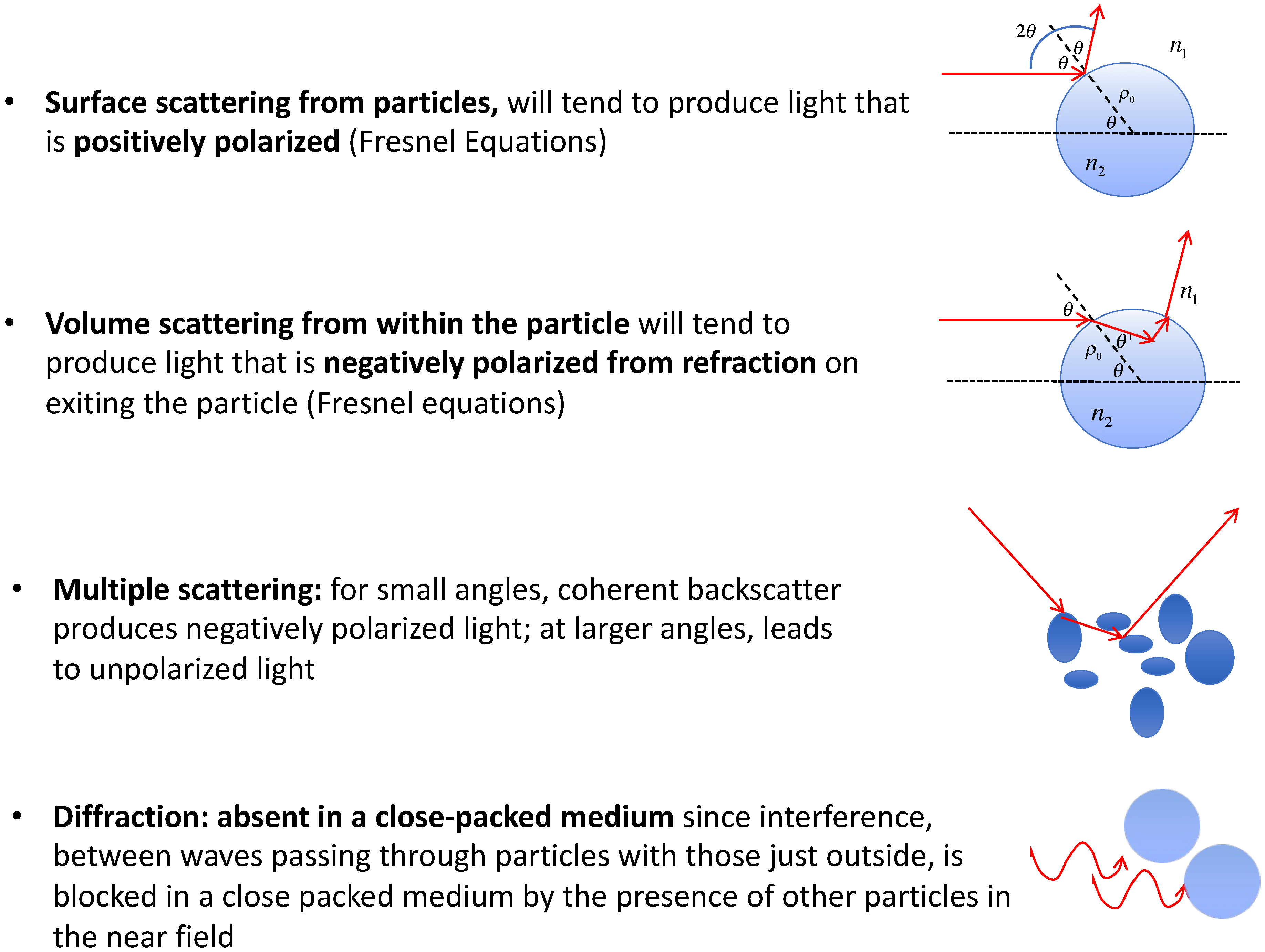
When a negative polarization branch exists, the typical minimum value in the negative branch is relatively small, ∼−0.01, at a phase angle below and the maximum value on the positive side is around 0.1 at approximately 100–110 [7]. Influences on polarization come from varying forms of scattering, as explained in Figure 1.
As Figure 1 illustrates, in a particulate medium, these observations stem from contributions due to surface scattering from particles (positively polarized light), volume scattering within particles (negatively polarized light), and multiple scattering between particles (negatively polarized light at small angles due to coherent backscatter effects [7,13], but otherwise unpolarized at larger angles). The coherent backscatter opposition effect (CBOE) has been well studied as one mechanism for the increased brightness at small phase angles observed in scattering from granular media, specifically at very small phase angles (typically ), and analysis and comparison with experiment suggest that low-order multiple scattering contributions (≤4 scattering events) typically contribute most at these small phase angles [7,13]. For light originating from a larger number of scattering events, the trend is toward randomization of the polarization, which in the aggregate leads to an unpolarized contribution. Figure 1 also illustrates that, as was observed previously, in a close-packed medium, diffraction effects can generally be ignored in the far field because interference in the near field is blocked by the presence of nearby particles [7].
Hapke developed a polarization model based on their Isotropic Multiple Scattering Approximation (IMSA) radiative transfer model [7], which will be discussed further in the next section. However, his model only focuses on the positive branch of polarization and does not agree with observational data at larger phase angles. This may be due in part to the assumptions made in model development, such as the neglect of negative polarization stemming from light transmitted through particles, the equal division of multiple scattering between the parallel and perpendicular radiance components, and the chosen isotropic form of multiple scattering used [7].
Prior to 1994, Shkuratov conceived several studies to model the negative branch in terms of different scattering phenomena. Shkuratov eventually summarized these models dividing them into 4 categories [8]. The first three are multiple reflection, refraction, and diffraction which were based on Lyot’s three hypotheses [8]. The final and most promising category used models of coherent backscatter.
This study examines the effect of grain size distribution on observed polarimetric hyperspectral reflectance data. The observed link between these provides insight that may help to improve models of polarization overall through analysis of physical parameters which impact polarization, allowing for better inversion and retrieval of these parameters. In our study, we focus on granular materials which may have both surface and volume scattering. In these materials, as noted above, the scattering mechanisms exhibited by granular materials, which appear in Figure 1, include multiple effects that contribute to the polarization. This contrasts with materials that exhibit primarily strong surface scattering and are better described by the Fresnel equations. While the impact of grain size on polarimetric data has been studied before by those mentioned above, here this relationship is studied using hyperspectral polarimetric data, giving much more insight into the wavelength dependence of polarimetric imagery of particulate surfaces. We also derive specific relationships between grain size and observed changes in an approximately linear region of the positive polarization branch.
2. Background
2.1. Hapke’s Model for the Positive Polarization Branch
Hapke’s solution to the radiative transfer equation, with the assumption of isotropic multiple scattering, is the basis for a model of the positive branch of polarization that matches observations for moderate phase angles [7]. Assuming phase angles greater than 20° and therefore neglecting opposition effects, the radiance solution is [7]:
where J is the incident irradiance, K is a nonlinear porosity function depending on the filling factor of the granular material, w is the wavelength-dependent single scattering albedo, is the single scattering phase function, dependent on phase angle g, H is the Ambartsumian-Chandrasekhar H-function [14] describing multiple scattering, is Hapke’s correction for macroscopic roughness [7,15], and are the effective incident and observation direction cosines of the locally tilted surface if the surface is rough and otherwise reduce to the incident and observation direction cosines of a flat surface in the absence of macroscopic roughness, and i and e denote the incident and observation zenith angles in a locally flat coordinate system [7]. Further details of the derivation can be found in [7]. More recent modeling efforts have provided more accurate models for macroscopic roughness [16]; however, as we will see below, the dependence on the macroscopic roughness factor is eliminated in the linear polarization ratio, although the direction cosines and that appear in the H-functions would be the effective direction cosines for a surface that is not smooth if macroscopic roughness is present. The multiple scattering term shown in Equation (2) is an isotropic form. As explained earlier, this equation can be further broken down into perpendicular and parallel components by assuming that the multiple scattering term is divided equally between the two, although this assumption is a potential reason for inconsistencies between the model and observations. The model parallel and perpendicular components are then [7]:
Combining these expression with Equation (1), one obtains the expression:
where depends on Fresnel coefficients, and , and an unpolarized residual term, , expressed in terms of the single scattering albedo:
where is the external surface reflection coefficient. The final resulting expression for polarization becomes [7]:
Further details can be found in [7].
While the model is conceptually straightforward, Hapke found that the model fails to predict the polarization maximum in observed data as well as the angle at which it occurs. This appears to be a limitation of the use of the Fresnel coefficients [7]. The difference between Fresnel coefficients in the numerator, and subsequently the polarization model as a whole, peaks at higher phase angles than in observational data [7]. This is increasingly true as the unpolarized residual term, , increases. Furthermore, this model does not accurately predict the polarization at phase angles greater than 80°, likely due to the approximate isotropic form of multiple scattering within the model. There is strong evidence that multiple scattering is not isotropic and is not evenly divided between the perpendicular and parallel orientations to the scattering plane. Furthermore, it may be necessary to insert the IMSA model into a Stokes’ matrix representation rather than reducing polarization information used to just two orientations. In addition, Equation (8) does not explicitly include particle size as a free parameter.
2.2. Models for the Negative Polarization Branch
Current models for the negative branch of polarization do not completely describe observations [7,8]. In addition to influencing the shape of the negative branch at small phase angles, negative polarization also likely plays a significant role at higher phase angles due to contributions from refracted light that enters particles but also escapes the particle in forward scattered directions. As Hapke has pointed out, such light will be negatively polarized [7]. At small phase angles near opposition, contributions likely stem from three sources: the coherent backscatter opposition effect (CBOE) [7,13], polarization opposition effect (POE) [7], and broad negative polarization (BNP) [7]. It is important to emphasize that these effects are expected for very fine particles [7] where the geometric optics model described earlier for the positive branch may not apply; however, even particles in the geometric optics regime may exhibit a negative polarization branch [7,8].
The negative branch is often bimodal, and the POE is the likely cause of the smaller-angle negative peak while BNP, which refers to the second peak, is not well understood [7]. Even the origin of the bimodal trend is uncertain, as the strength of the POE can be low. Quantitative understanding of the CBOE is somewhat developed, but virtually nonexistent for POE and the BNP. Even a qualitative understanding of BNP is lacking, other than its angular location very close to the angular region where the shadow-hiding opposition effect (increased reflectance) occurs at angles less than [7].
Several historical models were reviewed by Shkuratov [8]; however, since the majority of our data does not exhibit a negative polarization branch, likely due to larger particles sizes and lower bulk density, we limit our discussion here and refer the reader to Shkuratov’s earlier work [8] for further details on the experiments that he undertook to explore the limitations of these earlier models. His most successful models were based on coherent backscatter, which achieved better quantitative agreement with data. Among these, the more promising models were: (a) a second-order Fresnel reflection model with an exponential probability of light propagation between two scatterers and (b) a second-order point scatterer model based on a medium of small particles bounded by a plane and characterized by a single scattering albedo, a Rayleigh scattering phase function, and a ratio of particle radius to wavelength [8]. The first model predicts the wavelength dependence of polarization well, but would be difficult to apply practically to remote sensing imagery, while the second model, required significant simplification to match experimental data, and its use of a Rayleigh phase function limits applicability to very small particles. Other models, such as the discrete dipole approximation (DDA) [17], have been used to investigate, for example, the relationship between refractive index and the polarization minimum and its associated phase angle for irregular agglomerate particles, determining that the ratio of the phase angle to the cube of the real part of the refractive index remains constant [18]. Similarly, other studies using the same model have investigated the relationship between albedo and the polarization minimum [9]. Meanwhile, other works have examined the relationship between the polarization minimum and associated phase angle with variables such as particle size, index of refraction, and particle density and found that the polarization minimum is related to grain size, while also being influenced by these other variables [19].
2.3. Other Historical Models of Polarization
For small particles, a series of experimental studies by Kerker also explored the relationship of grain size and polarimetry [12], typically for small particles on a scale similar to the wavelength, such as aerosols and particles dissolved in solutions, where Mie scattering theory applies. Highly accurate experimental models were based on zero-order logarithmic distribution (ZOLD) functions [20] and incorporated multi-angular measurements to optimize models [12,21]. Similarly, other studies in the 1970s analyzed the wavelength dependence of polarization by observing interstellar grains [22]. These models assumed cylinders of constant length, a size distribution similar to the Oort-van de Hulst distribution, with refractive index m = 1.33 and orientation defined by the Davis-Greenstein mechanism [23] with orientation parameter 0.1–0.4. Their empirical polarization model form was
where was the polarization maximum average over the observational period. Their empirical model fit observations well and matched classical models over a wide range of for values of between 0.22 and 2.2 m [22]. A related grain size retrieval model was based on their observation that wavelength dependence of polarization played a more significant role than the absolute value of polarization, and that the nature of the grains of a surface could be narrowed down through the wavelength dependence of polarization [24].
Sun et al. compared the polarization of black soil to that of a particular type of sand (S2) [6]. Their experimental data covered wavelengths ranging from 300 to 2500 nm, and they grouped their sample particles into diameter ranges: 300 m or less, 300–450 m, 450 m, 450–900 m, and 900 m. Results showed that the black soil had more prominent positive and negative polarization peaks than the sand, for data in the spectral range 350–2300 nm. The results also suggested that negative polarization is more prominent for larger grain sizes than smaller ones, and that this relationship is more obvious with low-reflectance materials than high-reflectance materials [6], which is the opposite of what we found for the materials that we examined in this work.
3. Objectives
In this study, we analyze the impact of average grain size in granular materials on the observed polarization of hyperspectral imagery and use the observed trends to derive empirical relationships between grain size and polarization. Other parameters potentially influencing the polarization of spectral imagery include moisture level, material composition, and albedo. However, in this study, we focus on wavelength-dependent observations of grain size in materials of the same composition, observed using a hyperspectral imaging system [25]. Some progress was made by Shkuratov in identifying parameters that affect the negative polarization branch, but the nature of the relationship is still not well understood, and in this study, the materials analyzed did not exhibit a significant negative branch, likely due to the fact that the materials were representative of the geometric optics scattering regime in the observed wavelength range (400–100 nm) and were lower density having been sifted; Hapke and others previously found that bulk density is a determining factor for the presence of a negative branch, with more densely packed granular materials showing a strong negative branch and loosely packed materials exhibiting a minimal negative branch [7]. Many previous studies concentrated on materials where particle sizes were significantly smaller relative to the observation wavelengths, likely placing these materials in either the resonance regime or Rayleigh regime.
4. Methods
4.1. Materials and Equipment
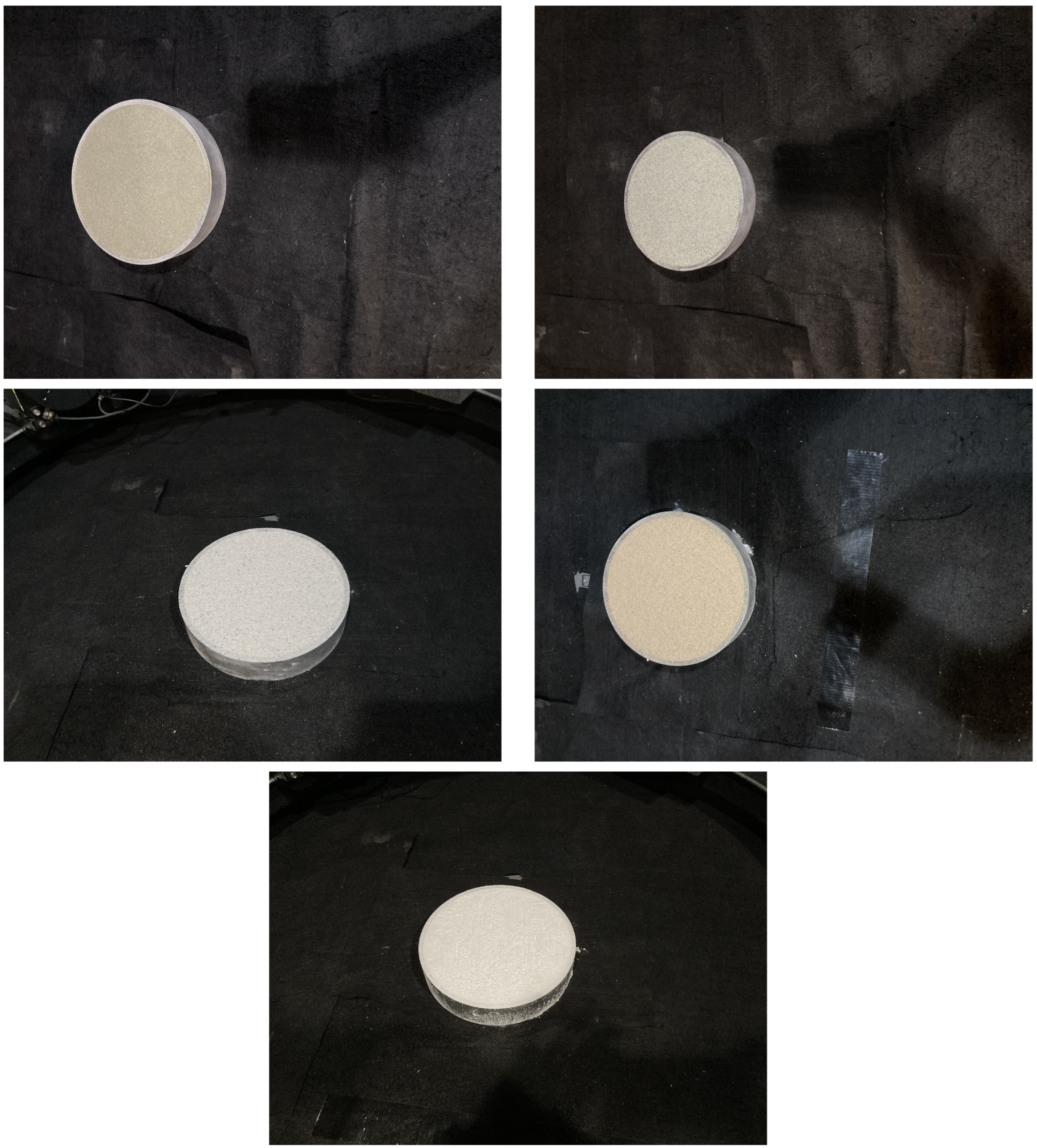
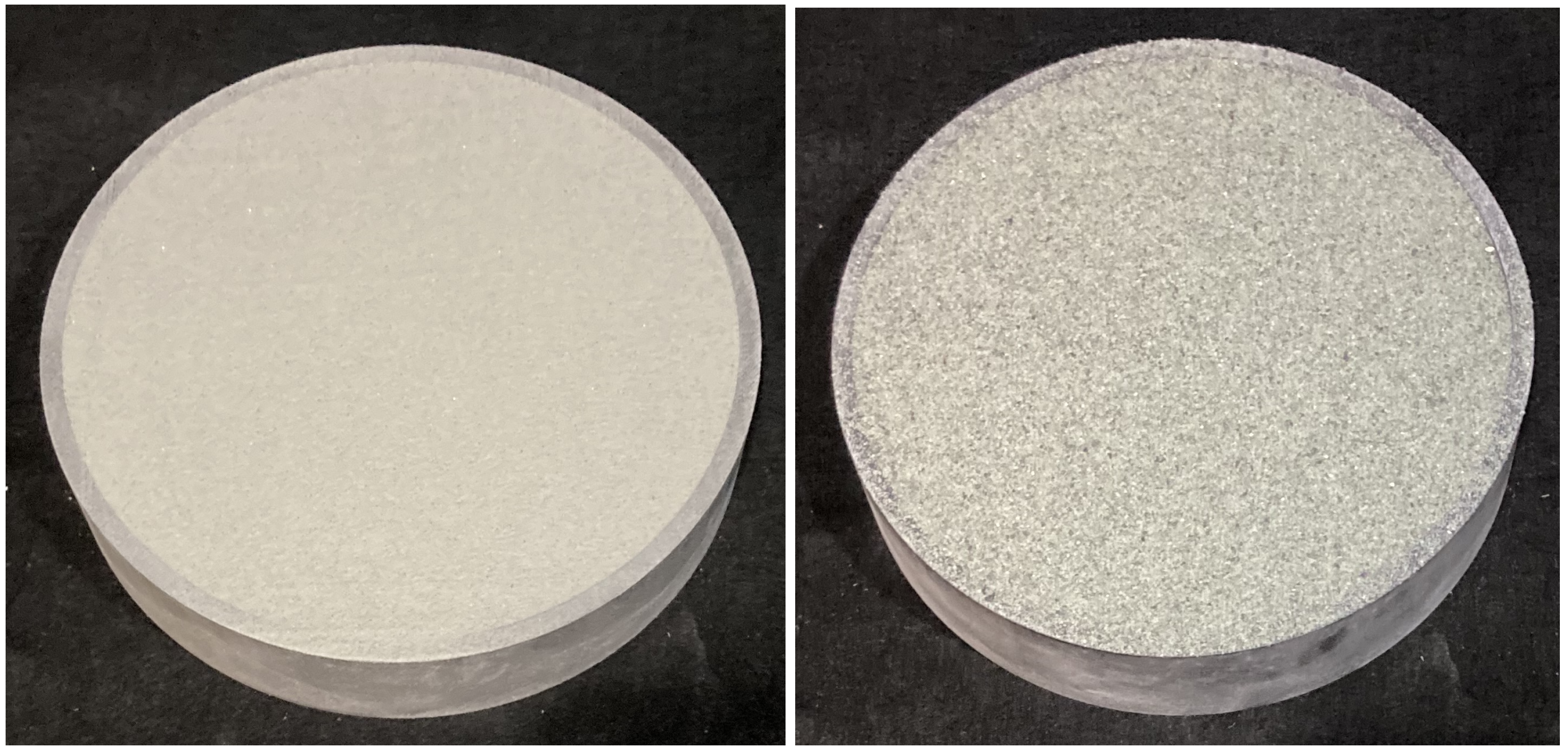
The samples analyzed in this experiment were olivine sediment with grain sizes ranging from 50 to 800 m provided by Washington Mills, and four samples provided by AGSCO, including an olivine sample with grain sizes ranging from 60 to 1000 m, a silica sample with grain sizes from 250 to 850 m, and two samples of nepheline sand, one with grain sizes ranging from 250 to 850 m and the other from 1 to 5 m. Because the grain sizes were comparable to the wavelength range of our hyperspectral imaging system (0.400–1.000 m), the latter sample fell within the resonance, or Mie scattering, regime, while the others, with significantly larger grain sizes, correspond to the geometric optics regime. Radiance measurements were also recorded from a standard white reference panel, but were not required to determine the linear polarization ratio used in this study. The samples corresponding to the geometric optics regime were sifted into multiple groups for grain size analysis. This provided a larger number of grain size categories to explore better the relationship between polarization and grain size. The specific grain size groupings appear in the Results section. We prepared the geometric optics regime samples in a black opaque circular container with a 20.32 cm diameter and a cardboard insert placed in the bottom of the container, making the sample depth 1.9 cm deep. We prepared the resonance regime sample without the insert so that the sample depth was 3.8 cm. Figure 2 shows example photographs of each AGSCO-prepared sample. Figure 3 highlights the difference between the AGSCO 63–300 m olivine and 600–1000 m olivine samples; these samples correspond to the largest contrast in grain size across samples used in our study, and the Figure highlights the obvious difference in material appearance due to differences in grain size.
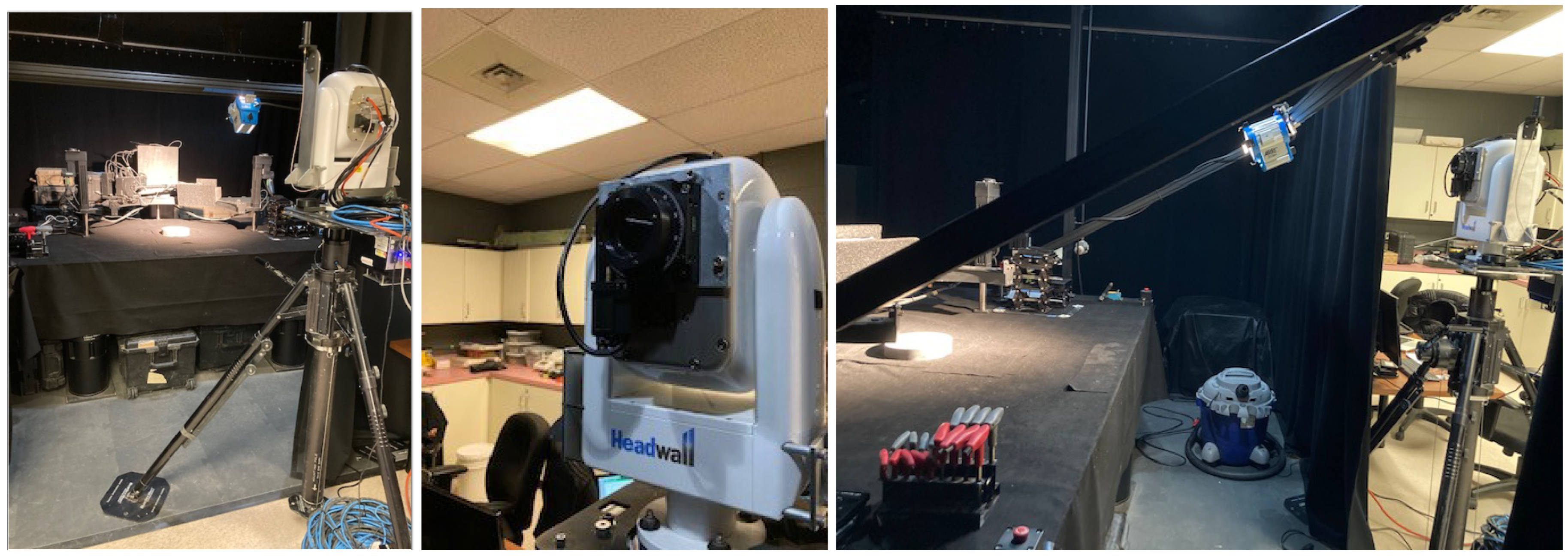
We collected hyperspectral imagery in our laboratory using a Headwall Hyperspec micro-HE (high efficiency) E-Series imaging system mounted on a General Dynamics pan-tilt unit [25]. A 50 mm polarizer was mounted at the front of the optical pathway [26]. The hyperspectral imaging system and polarizer both interface to a computer where their parameters can be managed. The polarizer is controlled through a stepper and DC motor controller and is mounted on a 360 deg rotation stage [27,28]. Within this configuration, the hyperspectral imaging system view geometry, polarizer angle, exposure, and field of view can be adjusted.
The hyperspectral imaging system collected imagery in 371 bands ranging from 400–1000 nm, sweeping from 15 to 30 deg below the horizontal. The Hyperspec is a pushbroom hyperspectral line scanner where the along-track spatial dimension is acquired by the motion of the imaging system. In an aircraft, this is generated by the platform motion, while in our system, the nodding of the pan-tilt unit produces the along-track spatial dimension [25]. This angular range placed the sample being analyzed in the center of the frame where it was also aligned with an unpolarized light source in the principal plane. For each data collection, we acquired hyperspectral imagery with the polarizer oriented at 0, 45, 90, and 135 degrees. The 0 and 90 deg orientations were used to calculate the linear polarization ratio using the raw digital count values of the two images, and the two oblique orientations were used as a test of the significance of adding those orientations associated with the other Stokes components. The light source is positioned on a transom attached to a rotation stage, which interfaces to a separate computer. To ensure that a wide range of phase angles could be measured, we rotated the illumination source via the rotation stage, changing the illumination zenith angle across a series of angular positions ranging between 25 and 135 deg with respect to the neutral position of the hyperspectral imaging system, with the light source increment being in 5 deg intervals. Figure 4 shows the lab setup from the point of view of our hyperspectral imaging system and from the side as well as the front of the hyperspectral imaging system with the polarizer attached.
A three-band image derived from one of the example hyperspectral images used in our study appears in Figure 5. In the Figure, approximately 3/4 of the output image width has been cropped, evenly on each side of the image, to remove the black background of our laboratory environment. The red, green, and blue bands appearing in the image represent wavelengths at 650.00 nm, 550.0231 nm, and 451.097 nm, respectively.
As shown, only a small portion of the image includes the sample itself, which necessitated masking of the background portions of the image. Our surrounding laboratory environment has black walls, ceiling panels, and flooring, and surrounding lights were shut off to minimize background light reaching the hyperspectral imaging system.
Additionally, the hyperspectral imaging system was calibrated by us using a LabSphere Helios integrating sphere [25], and these data were used to convert the raw digital numbers (DN) to radiance before calculating the polarization ratio.
4.2. Processing and Calculations
After collecting the data for each sample, a mask was developed in using a rectangular region of interest (ROI), which was manually drawn within the sample region of the image. Since the sample was not moved during each experiment, only one mask was needed for each data collection. The mask was specifically designed to exclude pixels close to the edge of the sample holder; however, the included portion contained a sufficient amount of data for analysis.
After creating the mask, the remaining processing and calculations were completed in Python. Images were read into Python, then the 0 and 90 deg polarizer orientations for each light angle were converted to radiance using the polarized calibration data. We acquired the calibration data using a 0.5 m HELIOS® 20 integrating sphere from Labsphere with an integrated 3000 K quartz tungsten halogen light source. We imaged the open port of the sphere with the Headwall imaging spectrometer with the affixed linear polarization stage. Specifically, we acquired radiance measurements using the calibrated spectrometer attached to the integrating sphere while simultaneously imaging the exit port of the sphere using the Headwall imaging spectrometer and linear polarizer configuration. Ten different illumination levels within the sphere were used to capture the full dynamic range of the Headwall imaging spectrometer at both and polarization angles. For our Headwall imaging system, the same exposure time of 100 ms used during the laboratory sample measurements was used for the integrating sphere calibration measurements. Using our calibration measurements, the digital number (DN) images of the particulate samples were then converted to calibrated radiance images, which were used to calculate the linear polarization ratio for each image pixel using Equation (1). The phase angle was calculated for each line of the image by subtracting the camera angle (which changes with the line number of the image) from the angle of the light source (which was changed for each set of four images at the aforementioned four polarizer orientations). Since the linear polarization ratio defined in Equation (1) is unitless, it was not theoretically necessary to convert raw DN values to radiance or reflectance; however, the use of calibrated radiance mitigates potential polarization bias, which could otherwise adversely affect the calculation of the linear polarization ratio in Equation (1). Tests were conducted comparing the results using the polarization ratio of Equation (1) to the results when using the 45 and 135 deg orientations as well in a Stokes analysis [29] where the polarization is defined as follows:
where:
Using the Stokes polarization that incorporated these additional polarization orientations did not significantly change the results. Therefore, the linear polarization ratio in Equation (1), using just two components, was sufficient for these samples.
After cropping out the background, the data were averaged along each line of the sample since the phase angle remains approximately constant along each line over the width of the sample holder. This step condensed the data significantly, improved the signal-to-noise ratio (SNR), and allowed for ease of analysis. Polynomial curves of varying orders were then fit to this averaged data to determine the most appropriate model based on the root mean squared error (RMSE). Finally, the slope of the linear region of the data was plotted against the average grain size of each measured sample. Further details of the analysis appear in the next section.
5. Results and Discussion
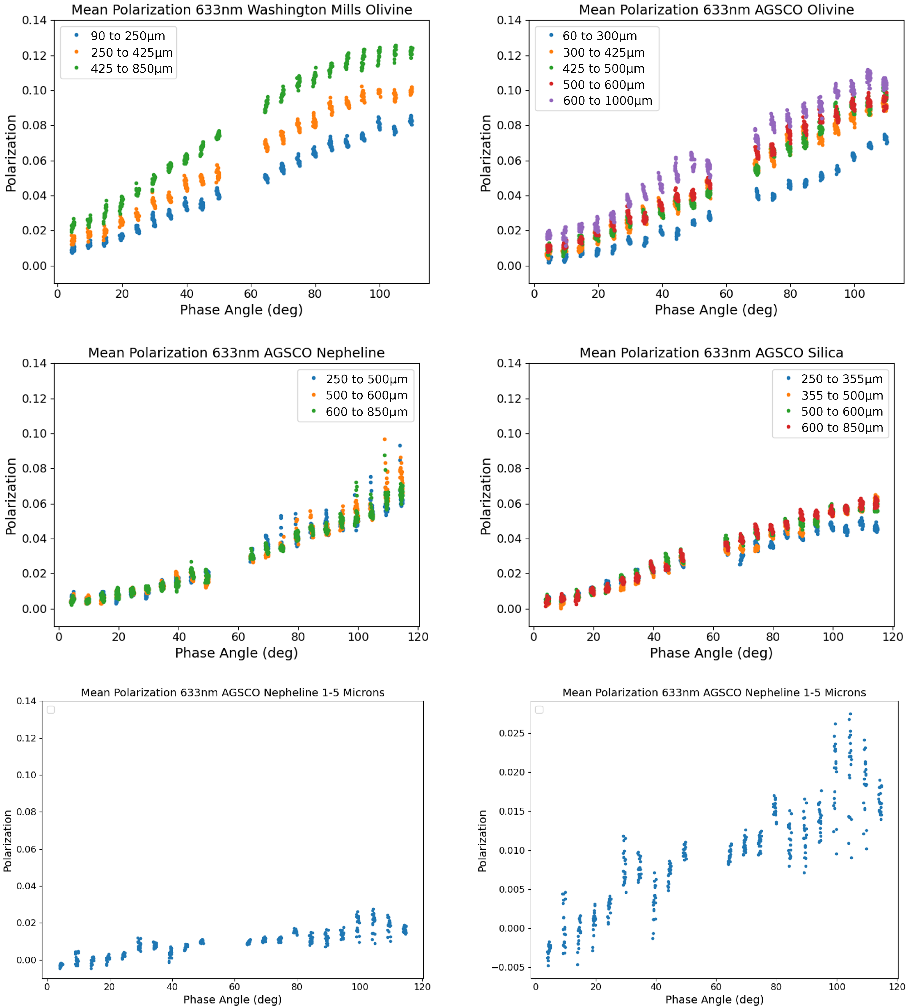
Figure 6 shows the linear polarization ratio for a representative wavelength (633 nm) for each sample measured, averaged along each line of the sample in the image data as described earlier, with one mean value in the plot for every row of the image after masking out the background. As shown, the olivine from Washington Mills displays a much more distinct separation and trend as a function of grain size than the other geometric-optics regime samples, including the AGSCO olivine. However, the AGSCO olivine does have narrower steps between grain size categories than the Washington Mills olivine, so the behavior might have been more similar if the samples could have been binned the same way, and we note that the separation in polarization between the largest and smallest grains is actually similar between the two olivine samples. The AGSCO olivine, however, does have more separation than the nepheline or silica. This may be due to a combination of differences in material properties and the specific grain size categories chosen. The Washington Mills olivine shows a much greater increase in the polarization maximum with increasing grain size than the other samples, for which the maximum increases more gradually. The reason for this will require further study. However, when we examine the best-fit polynomials to each curve in Figure 7, every sample among the geometric optics regime-sized samples shows some separation between curves for the different grain sizes at phase angles of 45 deg or higher.
The final plots in Figure 6 and Figure 7 show the nepheline sample with resonance regime-sized particles. Here, the particle size distribution is better described by Mie Scattering due to the relative size of the particles compared to the wavelength. Because of its distinct behavior, in Figure 6, a version of these data is shown with a zoomed-in scale to provide greater detail. A point of interest is that the curve for this sample is significantly flatter beyond a phase angle of 30 deg than for the other samples. None of the samples showed a negative polarization branch, except for the resonance regime-sized sample below a phase angle of . This is in line with Shkuratov’s results for resonance-sized samples. We return to this observation in our discussion of the results later in this section.
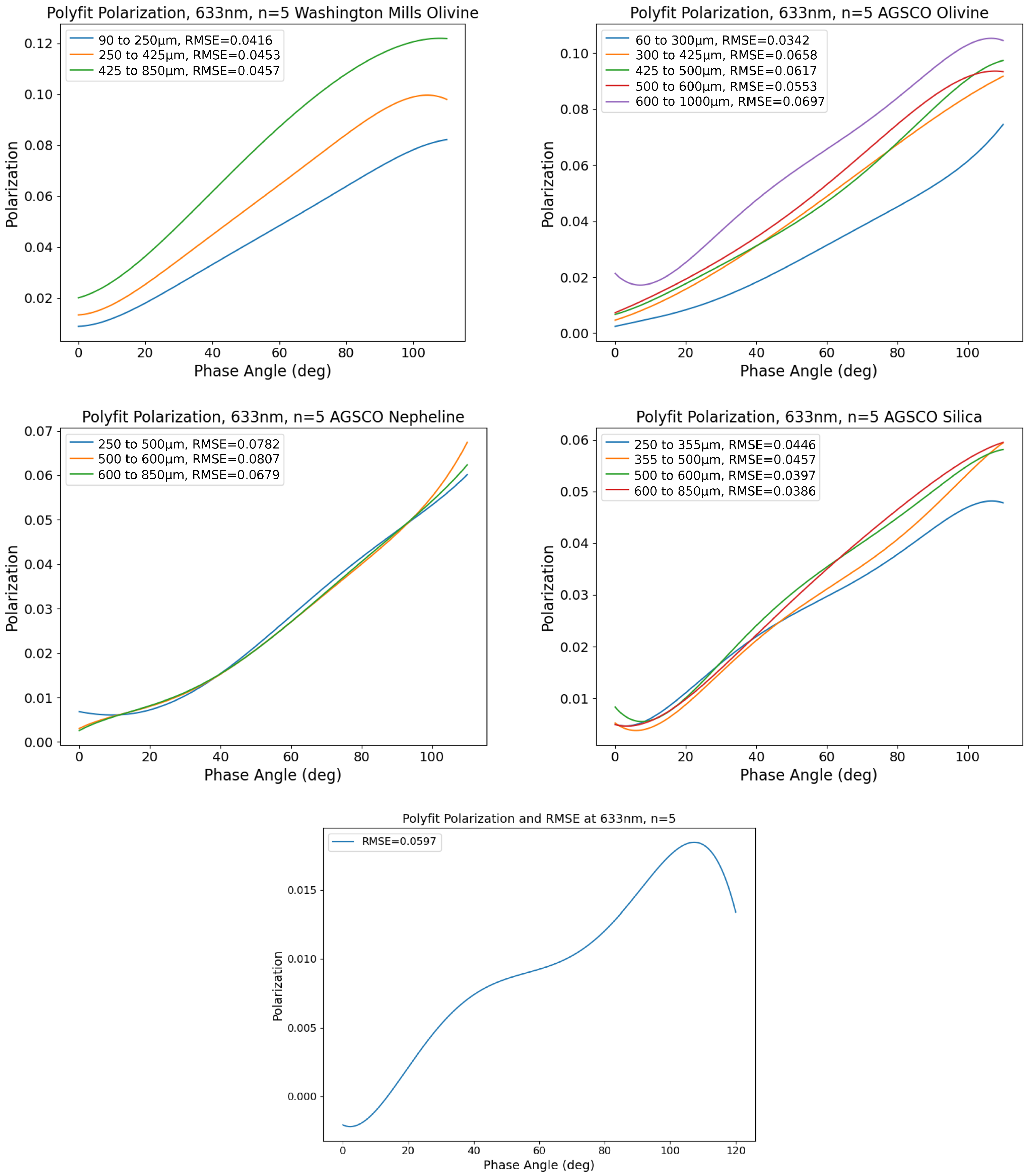
Figure 7 shows a 5th-order polynomial fit to each of the datasets appearing in Figure 6. This offers an easier analysis of the behavior of the data in the macro scale, i.e., across the full range of phase angles. The general trend for the Washington Mills olivine remains consistent for the averaged data across the different grain size distributions; however, the slope increases significantly as grain size increases. In contrast, the other geometric-optics regime samples all have grain size-designated curves that intersect the other curves more than once. On the other hand, consistent with the Washington Mills olivine sample, the other geometric optics regime samples each have regions in which there is increasing polarization with grain size. The resonance sized sample is entirely distinct, even having a negative polarization branch and multiple significant slope changes.
Figure 7 also shows the RMSE of fifth-order polynomial fits to the data sets. The fits to linear polarization with phase angle did not exhibit significant wavelength dependence and had comparable RMSE provided wavelengths were sufficiently far from the edges of the spectral range of the imaging system, avoiding lower signal-to-noise (SNR) regions of the imaging system. In our study, we found satisfactory data quality between 400 and 900 nm. Additionally, the necessary order of the model to achieve sufficient accuracy did not vary significantly with different grain size ranges within a sample. First, second and third-order fits were also considered, but had higher RMSE, while fifth-order fits captured the data most accurately. Fifth-order polynomial fits may not be sufficient to model samples displaying measurements taken at higher phase angles than the maximum range measured in this study (120 deg). Orders higher than 5 were tested and found to be unnecessary for the range of phase angles measured in our study, as these higher orders did not noticeably decrease the RMSE.
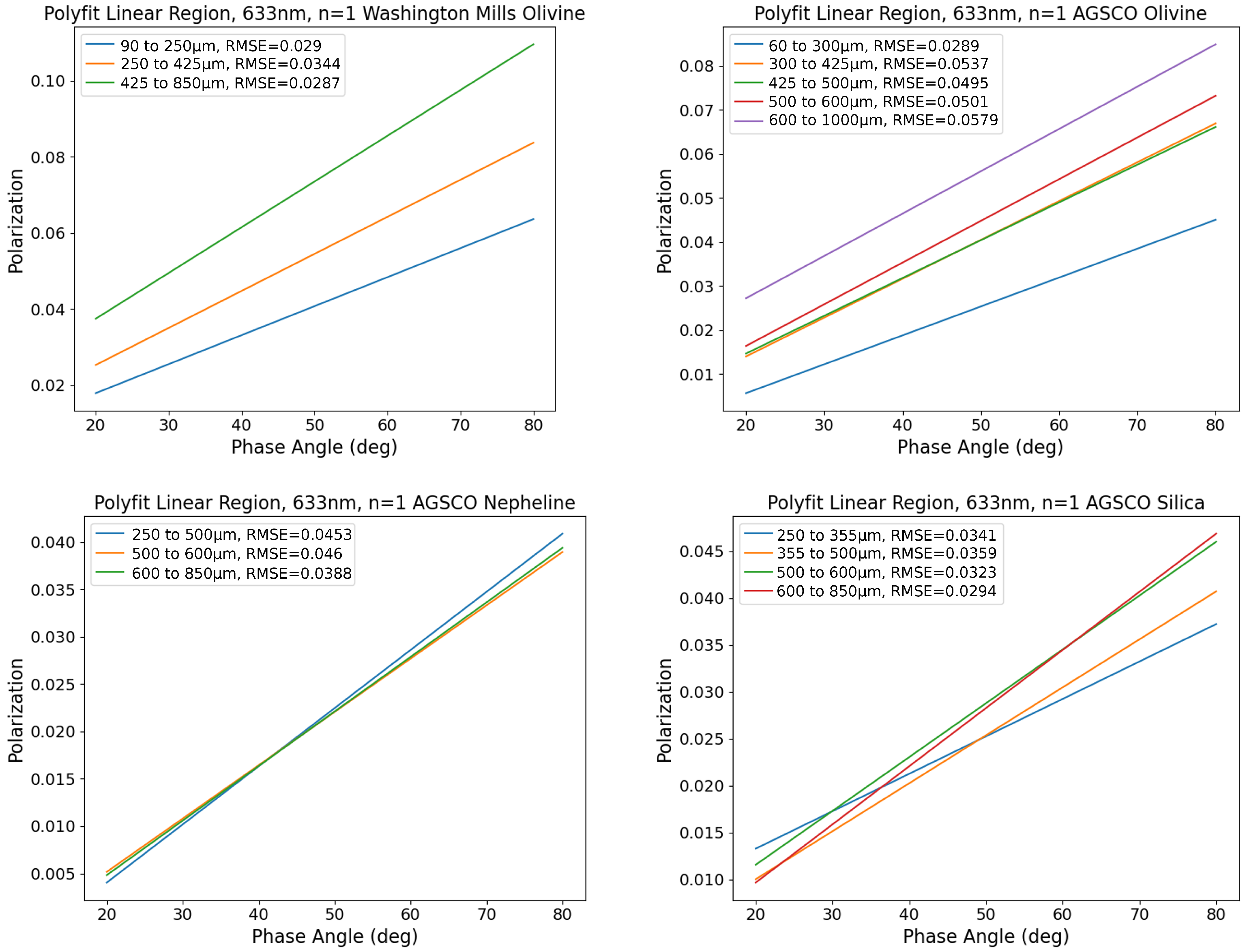
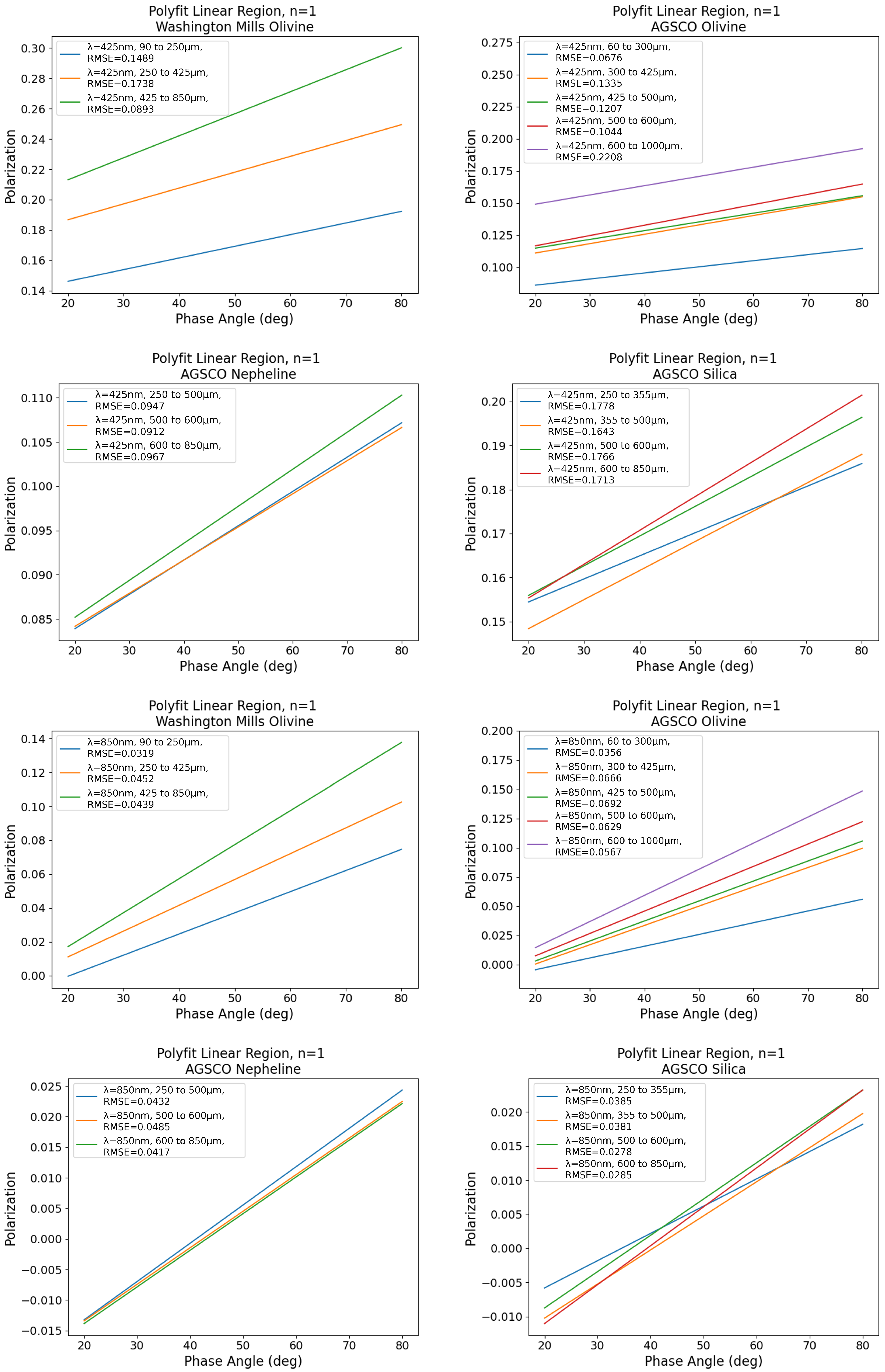
In addition to the trends already discussed, our measurements indicated a region of the polarization curve which was linear between phase angles of 20 and 80 deg for all of the samples considered. A linear fit at a wavelength of 633 nm for each sample appears in Figure 8, and for 425 and 850 nm in Figure 9, demonstrating the consistency of this trend across the wavelength range. Figure 8 shows these fits to be as accurate as the fifth order fits to the full-range data in Figure 6, and additional analysis not shown in this paper proved that the RMSE is not significantly changed between a linear fit and the fifth order curve fit within the 20–80 deg region, suggesting that this region is basically linear.
Figure 9 demonstrates that the RMSE of linear fits of data is still sufficient at 850 nm. For some of the samples, there is an increase in RMSE at 425 nm compared to the other two wavelengths shown, possibly because the 425 nm wavelength is too close to the lower end of the spectral range where SNR is lower. Nevertheless, a linear region was still observed at even those wavelengths at the extreme end of the spectral range (i.e., the RMSE even at 425 nm was not significantly worse for a linear vs. 5th order curve fit).
We analyzed the impact of grain size, wavelength, and material type on the slope of the linear region. The results are shown for each respective material type in Table 1. The Table shows that, to some degree, this slope varies with all three of the aforementioned properties. The one material which has a different trend, compared to the others, is the nepheline sample. As we discuss later, this material appears to be more strongly surface scattering than the other materials, which may have led to some of the apparent differences. We analyze these differences further below.
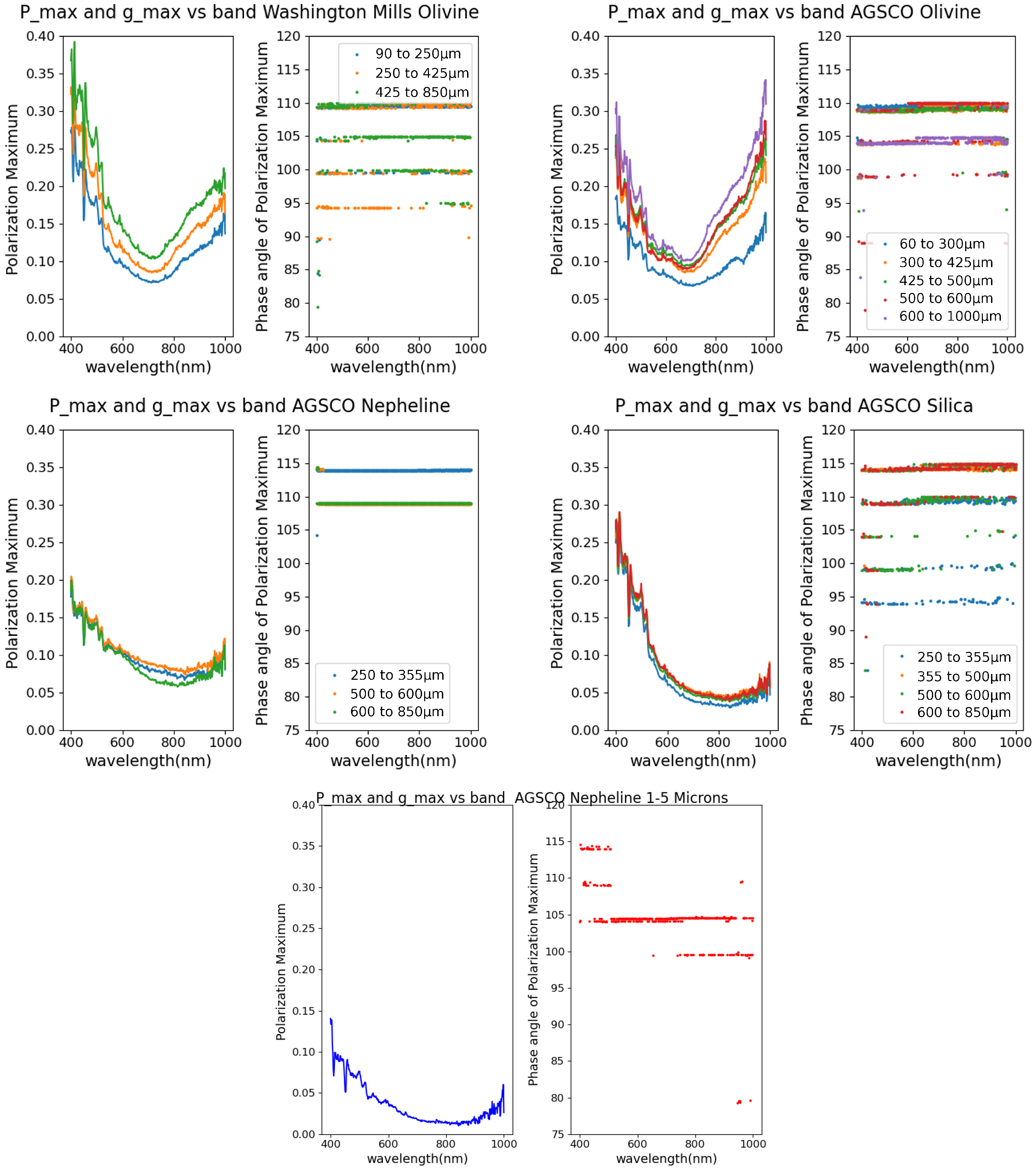
At each wavelength, we extracted a single maximum value for the average polarization along with the corresponding phase angle at each wavelength. The results appear in Figure 10. For the silica and nepheline samples, the lowest value of the polarization maximum occurs near 810 nm. Physically this wavelength corresponds to a local minimum of water absorption [30]. Although all samples were dried in an oven prior to measurement, hygroscopic absorption could still play a role, and this feature near 810 nm may indicate that hygroscopic moisture might be present in the sample data. However, this lowest value of the polarization maximum is in a broad minimum in the silica and nepheline plots, and we also observe that the lowest value of the polarization maximum for the olivine samples is closer to 700 nm, which also casts doubt on the presence of hygroscopic moisture.
In Figure 10, we see that the phase angle of the maximum falls generally within the 100–120 range predicted by theory, excluding the noise in some of the samples. For the typical indices of refraction of the materials used in this study, the Fresnel equations predict a polarization maximum in this range. We also observe that the phase angle of the linear polarization ratio maximum of these samples is only very weakly correlated with wavelength in some of the materials measured; instead, the phase angle of the maximum appears to be at certain discrete levels. The phase angle of the maximum has some weak correlation with grain size, but the degree to which this is true varies with the material.
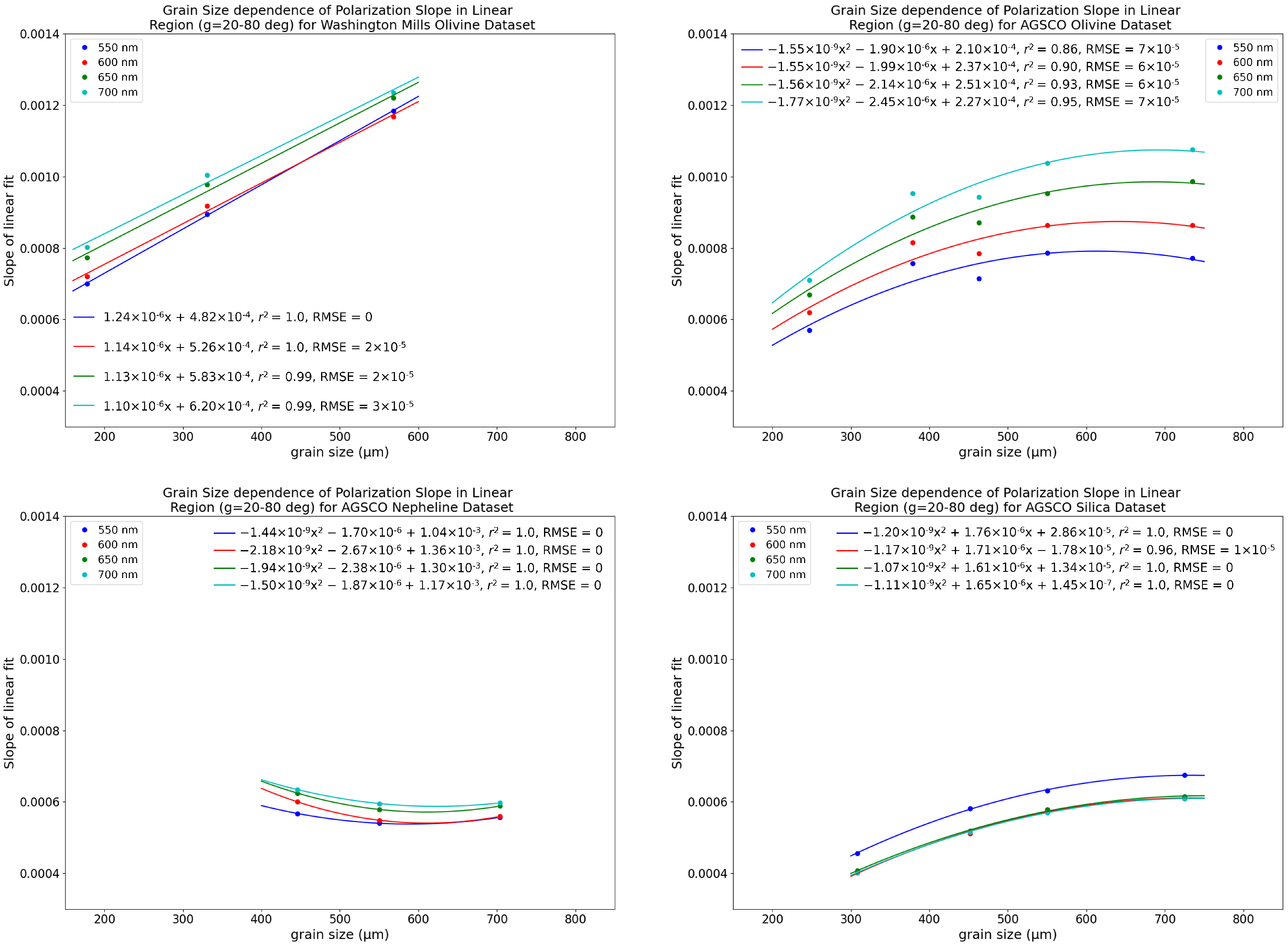
For each sample, we also analyzed the impact of the average grain size on the slope of the linear region of the polarization curve for each sample. The results appear in Figure 11. To illustrate the trends, we calculated slopes of the linear region of the polarization curves for four representative wavelengths at even intervals in the middle of the spectral range of the hyperspectral imaging system. Figure 11 shows the slope of the linear region of the sample data for the average grain size of each sifted sample for each material. Plots appear in this Figure for each of the four example wavelengths in the spectral range of the hyperspectral imaging system. Comparing linear and quadratic models, we found that quadratic fits had the lowest RMSE and best values for all samples, with the exception of the Washington Mills olivine for which a linear model was sufficient. In all cases, the goodness of fit ranged between 0.85 and 1.0. However, one notable distinction is the difference in the concavity of the AGSCO nepheline quadratic fit compared to the quadratic fits obtained for the AGSCO olivine and AGSCO silica samples. Material properties or potentially even particle shape may play a role in this. Since nepheline is highly reflective over a broad range of wavelengths with grains that visually exhibit glint and sparkle, there is likely greater surface scattering and less volume scattering and absorption in this material compared to the others used in our study. Also, the impact of grain size on the slope of the linear region appears to be much stronger for olivine, though the order of the relationship was inconsistent between the two olivine samples.
To elaborate, as noted in Figure 1, surface scatter will tend to increase polarization while light that has been transmitted through particles and emerges from the particle will tend to be negatively polarized. In particular, the amount of negatively polarized light emerging from particles will depend on the particle diameter because the mean ray path, or average transit length through a particle, should be directly proportional to particle diameter. The theoretical basis of this argument is an equivalent slab model for particle absorption and transmission discussed by Hapke [7]. In his model, the mean ray path is proportional to the average particle diameter D:
where represents the real part of the index of refraction of the material relative to the surrounding medium (in this case air). Thus, the contribution of negatively polarized light that has been transmitted should be expected to decrease as particles grow larger and extinction increases with the longer average path within the particle. This leads to an increasing polarization maximum as particles increase in size, which is the effect that we observe in Figure 6. The increased peak translates also to a steeper slope in the approximately linear region of the polarization curves between 20–80, and thus the observed correlation and increase in the slope in this region as grain size increases; we observe this trend for all but the nepheline sample, which had significantly smaller particle sizes, and for which as noted earlier, the particles are likely dominated by surface scattering rather than volume scattering.
Returning to the question of why no negative branch of polarization was observed in the geometric optics regime samples, it seems likely that the absence of a negative branch may also be related to a similar mechanism. In backscattered light, especially close to the opposition direction with phase angles less than where the negative branch would be observed if present, light that has been reflected from the surface will be positively polarized, while contributions from light that refract into the particle and then are scattered backward within the volume or from somewhere in the interior surface eventually emerging from the particle, would be negatively polarized. However, in larger particles, this latter contribution from light scattering from the particle volume or interior particle surface and eventually emerging from the particle in a direction toward a sensor positioned at smaller phase angles (<20) will diminish with longer mean ray paths and therefore greater extinction. Thus, larger particles will have greater polarization and may not have a negative polarization branch at all, which is what we observed in our samples. In the case of the sample with smaller 1–5 m nepheline particles, that are in the resonance regime, this contribution may be as small as it is because the material has such strong surface scattering, which is positively polarized, leading to the observed very small scale of the negative branch of linear polarization observed below .
The particulate samples in our analysis were illuminated with a directional source in a controlled laboratory setting. Although this illumination geometry simulates direct sunlight, skylight also contributes to the illumination in outdoor field conditions. Skylight is highly polarized due to Rayleigh scattering, and the polarization of the sky is dependent on the local Sun angles, the distribution of aerosol scatterers, and other atmospheric parameters. For bluer wavelengths, we estimated diffuse illumination in past field experiments by measuring the radiance from a shaded Spectralon panel and found that this radiance is approximately 30% compared to that from an unshaded Spectralon panel. For longer wavelengths past 450 nm, this value drops to 3–5%; therefore, we could expect samples illuminated in outdoor environments to be more similar in longer wavelengths to our present laboratory analysis. The effect of skylight illumination, which is also polarized, on the polarimetry of the scene is a complex problem.
6. Conclusions
Our results demonstrate a wavelength-dependent relationship between polarization and grain size. However, the grain size relationship appears largely material-dependent. Thus, direct measurement or estimation of the parameters of single scattering albedo, material purity, and index of refraction could expand the usefulness of these results. A rigorous model for the observed relationship is still to be developed; however, we have provided a physical motivation for understanding the results obtained thus far. For most of the materials measured, the slope of the polarization curve increases in the region where the polarization curve is approximately linear between phase angles of 20–80. We argued that this can be directly linked to the increasing size of the mean ray path which governs the amount of negatively polarized light that can escape from particle volumes. Past theoretical work by Hapke [7] based on an equivalent slab model of particle absorption and transmission indicates a linear dependence of the mean ray path on typical particle diameter. When typical particle size increases, therefore, we can expect the amount of negatively polarized light available from transmission through particles should decrease, therefore raising the polarization maximum and increasing the slope in the linear region of the polarization curve as average particle size increases. We observed this behavior in all but one material, the nepheline sample, which differed from the rest because scattering from this material was likely dominated by surface scattering, and this behavior likely also led to the much-reduced scale of its negative branch of polarization. For all of the materials, fits between the slope of the polarization data in the linear region between and and the average grain size obeyed either a linear or quadratic relationship with values between 0.855 and 1.00. While we described a plausible mechanism for understanding why these relationships exist, a comprehensive model of the connection between polarization and its correlation with grain size and other geophysical parameters remains a longer-term objective since it has important implications for remote sensing applications. Future studies could explore additional geophysical parameters other than grain size, how this type of data might differ if organic sediments were included, and the impact of skylight or different types of light sources.
Author Contributions
Conceptualization, R.M.G. and C.M.B.; methodology, R.M.G. and C.M.B.; software, R.M.G., C.S.L. and C.H.L.; hardware integration, C.S.L.; validation, R.M.G. and C.M.B.; formal analysis, R.M.G. and C.M.B.; investigation, R.M.G. and C.M.B.; resources, C.M.B.; data curation, R.M.G., C.H.L. and C.S.L.; writing—original draft preparation, R.M.G. and C.M.B.; writing—review and editing, R.M.G., C.M.B. and C.H.L.; visualization, R.M.G. and C.M.B.; supervision, C.M.B.; project administration, C.M.B. All authors have read and agreed to the published version of the manuscript.
Funding
This research received no external funding.
Data Availability Statement
The laboratory data and Python code used to implement these roughness correction models can be found at https://www.doi.org/10.35009/cfccis-8w70 (accessed on 10 July 2023).
Conflicts of Interest
The authors declare no conflict of interest.
Abbreviations
The following abbreviations are used in this manuscript:
| Polarization Opposition Effect | POE |
| Zeroth Order Logarithmic Distribution | ZOLD |
| Coherent Backscatter Opposition Effect | CBOE |
| Broad Negative Polarization | BNP |
| Direct Current | DC |
| NIR | Near Infrared |
| nanometers | nm |
| BRDF | Bidirectional Reflectance Distribution Function |
| Region of Interest | ROI |
| Digital Number | DN |
| Signal-to-Noise Ratio | SNR |
| Root Mean Squared Error | RMSE |
| Coefficient of Determintation |
References
- Martin, J.A.; Gross, K.C. Estimating index of refraction from polarimetric hyperspectral imaging measurements. Opt. Express 2016, 24, 17928–17940. [Google Scholar] [CrossRef] [PubMed]
- Gilerson, A.; Carrizo, C.; Ibrahim, A.; Foster, R.; Harmel, T.; El-Habashi, A.; Lee, Z.; Yu, X.; Ladner, S.; Ondrusek, M. Hyperspectral polarimetric imaging of the water surface and retrieval of water optical parameters from multi-angular polarimetric data. Appl. Opt. 2020, 59, C8–C20. [Google Scholar] [CrossRef]
- Hannadige, N.K.; Zhai, P.W.; Gao, M.; Franz, B.A.; Hu, Y.; Knobelspiesse, K.; Werdell, P.J.; Ibrahim, A.; Cairns, B.; Hasekamp, O.P. Atmospheric correction over the ocean for hyperspectral radiometers using multi-angle polarimetric retrievals. Opt. Express 2021, 29, 4504–4522. [Google Scholar] [CrossRef] [PubMed]
- Sun, Z.; Zhao, Y. The effects of grain size on bidirectional polarized reflectance factor measurements of snow. J. Quant. Spectrosc. Radiat. Transf. 2011, 112, 2372–2383. [Google Scholar] [CrossRef]
- Sun, Z.; Wu, D.; Lv, Y. Optical Properties of Snow Surfaces: Multiangular Photometric and Polarimetric Hyperspectral Measurements. IEEE Trans. Geosci. Remote Sens. 2021, 60, 4301516. [Google Scholar] [CrossRef]
- Sun, Z.; Zhang, J.; Tong, Z.; Zhao, Y. Particle size effects on the reflectance and negative polarization of light backscattered from natural surface particulate medium: Soil and sand. J. Quant. Spectrosc. Radiat. Transf. 2014, 133, 1–12. [Google Scholar] [CrossRef]
- Hapke, B. Theory of Reflectance and Emittance Spectroscopy; Cambridge University Press: Cambridge, UK, 2012. [Google Scholar]
- Shkuratov, Y.G.; Muinonen, K.; Bowell, E.; Lumme, K.; Peltoniemi, J.; Kreslavsky, M.; Stankevich, D.; Tishkovetz, V.; Opanasenko, N.; Melkumova, L.Y. A critical review of theoretical models of negatively polarized light scattered by atmosphereless solar system bodies. Earth Moon Planets 1994, 65, 201–246. [Google Scholar] [CrossRef]
- Shkuratov, Y.; Opanasenko, N.; Opanasenko, A.; Zubko, E.; Bondarenko, S.; Kaydash, V.; Videen, G.; Velikodsky, Y.; Korokhin, V. Polarimetric mapping of the Moon at a phase angle near the polarization minimum. Icarus 2008, 198, 1–6. [Google Scholar] [CrossRef]
- Fresnel, A. Oeuvres Complètes d’Augustin Fresnel; Imprimerie Impériale: Paris, France, 1868. [Google Scholar]
- Lyot, B. Recherches sur la Polarisation de la Lumière des Planètes et de Quelques Substances Terrestres; Observatoire de Paris: Paris, France, 1929. [Google Scholar]
- Kerker, M. The Scattering of Light and Other Electromagnetic Radiation: Physical Chemistry: A Series of Monographs; Academic Press: Cambridge, MA, USA, 2013; Volume 16. [Google Scholar]
- Hapke, B. Bidirectional reflectance spectroscopy: 5. The coherent backscatter opposition effect and anisotropic scattering. Icarus 2002, 157, 523–534. [Google Scholar] [CrossRef] [Green Version]
- Chandrasekhar, S. Radiative Transfer; Dover Publications: New York, NY, USA, 1960. [Google Scholar]
- Hapke, B. Bidirectional reflectance spectroscopy. 3. Correction for macroscopic roughness. Icarus 1984, 59, 41–59. [Google Scholar] [CrossRef] [Green Version]
- Shiltz, D.J.; Bachmann, C.M. An alternative to Hapke’s macroscopic roughness correction. Icarus 2022, 390, 115240. [Google Scholar] [CrossRef]
- Draine, B.T.; Flatau, P.J. Discrete-dipole approximation for scattering calculations. Josa A 1994, 11, 1491–1499. [Google Scholar] [CrossRef] [Green Version]
- Zubko, E.; Videen, G.; Shkuratov, Y. Retrieval of dust-particle refractive index using the phenomenon of negative polarization. J. Quant. Spectrosc. Radiat. Transf. 2015, 151, 38–42. [Google Scholar] [CrossRef]
- Zubko, E.; Muinonen, K.; Shkuratov, Y.; Videen, G. Negative polarization of agglomerate particles with various densities. In AAPP Atti della Accademia Peloritana dei Pericolanti-Classe di Scienze Fisiche, Matematiche e Naturali; Accademia Peloritana dei Pericolanti: Messina, Italy, 2011; Volume 89. [Google Scholar]
- Espenscheid, W.; Kerker, M.; Matijević, E. Logarithmic Distribution Functions for Colloidal Particles1a. J. Phys. Chem. 1964, 68, 3093–3097. [Google Scholar] [CrossRef]
- Kerker, M.; Daby, E.; Cohen, G.; Kratohvil, J.; Matijevic, E. Particle size distribution in La Mer sulfur sols. J. Phys. Chem. 1963, 67, 2105–2111. [Google Scholar] [CrossRef]
- Coyne, G.; Gehrels, T.; Serkowski, K. Wavelength dependence of polarization. XXVI. The wavelength of maximum polarization as a characteristic parameter of interstellar grains. Astron. J. 1974, 79, 581–589. [Google Scholar] [CrossRef]
- Davis Jr, L.; Greenstein, J.L. The polarization of starlight by aligned dust grains. Astrophys. J. 1951, 114, 206. [Google Scholar] [CrossRef]
- Gehrels, T. Wavelength dependence of polarization. XXVII. Interstellar polarization from 0.22 to 2.2 μm. Astron. J. 1974, 79, 590–593. [Google Scholar] [CrossRef]
- Bachmann, C.M.; Eon, R.S.; Lapszynski, C.S.; Badura, G.P.; Vodacek, A.; Hoffman, M.J.; McKeown, D.; Kremens, R.L.; Richardson, M.; Bauch, T.; et al. A Low-Rate Video Approach to Hyperspectral Imaging of Dynamic Scenes. J. Imaging 2019, 5, 6. [Google Scholar] [CrossRef] [Green Version]
- Edmund Optics 50 mm Ultra-Broadband Wire Grid Linear Polarizer. Available online: https://www.edmundoptics.com/p/50mm-ultra-broadband-wire-grid-linear-polarizer/3701/ (accessed on 29 July 2021).
- Standa 8SMC5-USB—Stepper & DC Motor Controller. Available online: http://www.standa.lt/products/catalog/motorised_positioners?item=525 (accessed on 29 July 2021).
- Standa 8MR190-2—Motorized Rotation Stage. Available online: http://www.standa.lt/products/catalog/motorised_positioners?item=244 (accessed on 29 July 2021).
- De Boer, J.F.; Milner, T.E. Review of polarization sensitive optical coherence tomography and Stokes vector determination. J. Biomed. Opt. 2002, 7, 359–371. [Google Scholar] [CrossRef]
- Curcio, J.A.; Petty, C.C. The near infrared absorption spectrum of liquid water. JOSA 1951, 41, 302–304. [Google Scholar] [CrossRef]
Figure 1.
Scattering influences on the observed polarization in granular media. In close-packed media, principle contributions stem from: (top) surface scattering, (upper middle) volume scattering within particles, (lower middle) multiple scattering between particles. (Bottom) Diffraction effects can generally be ignored in the far field.

Figure 2.
Photos of prepared samples of 250–425 m olivine from Washington Mills (top left), and from AGSCO 500–600 m olivine (top right), 500–600 m nepheline (middle left), 500–600 m silica (middle, right), and 1–5 m nepheline (bottom).
Figure 2.
Photos of prepared samples of 250–425 m olivine from Washington Mills (top left), and from AGSCO 500–600 m olivine (top right), 500–600 m nepheline (middle left), 500–600 m silica (middle, right), and 1–5 m nepheline (bottom).

Figure 3.
Photos of prepared samples of AGSCO 63–300 m olivine (left) and 600–1000 m olivine (right).
Figure 3.
Photos of prepared samples of AGSCO 63–300 m olivine (left) and 600–1000 m olivine (right).

Figure 4.
(Left) Experimental Setup from point of view of the hyperspectral imaging system, (middle) the hyperspectral imaging system with the polarizer and rotation stage attached, (right) side view of the experimental configuration.
Figure 4.
(Left) Experimental Setup from point of view of the hyperspectral imaging system, (middle) the hyperspectral imaging system with the polarizer and rotation stage attached, (right) side view of the experimental configuration.

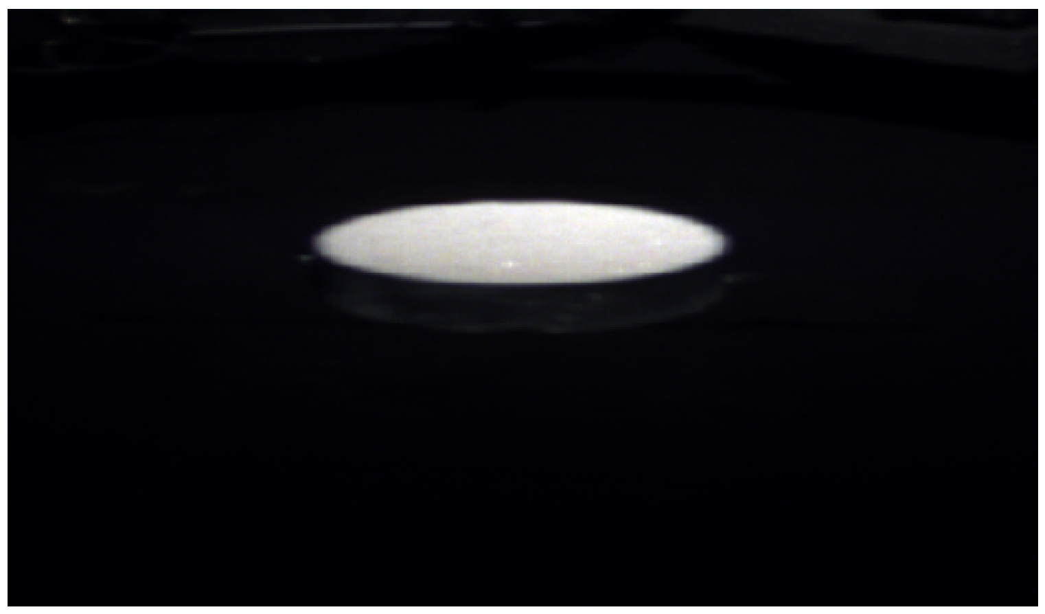
Figure 5.
Example hyperspectral Raw DN output image for a 500–600 m Nepheline sample with polarizer zenith angle of 0 deg and illumination zenith angle of 50 deg. Displayed RGB bands selected from the hyperspectral imagery are, respectively, band 156 (650.99 nm), band 94 (550.231 nm), and band 33 (451.097 nm).

Figure 6.
Average linear polarization of each hyperspectral image sample line for grain size subsets: (top left) Washington Mills olivine; (top right) AGSCO olivine; (middle left) AGSCO nepheline; (middle right) AGSCO silica; (bottom left) AGSCO resonance regime-sized nepheline on the same scale as other samples; (bottom right) AGSCO resonance-regime nepheline on a scale matched to the dynamic range of the data.

Figure 7.
Fifth order polynomial fits to averaged linear polarization vs. phase angle with RMSE for binned samples of various grain sizes: (top left) Washington Mills olivine grain sizes between 90–250 m, 250–425 m, and 425–850 m; (top right) AGSCO olivine between 60–300 m, 300–425 m, 425–500 m, 500–600 m, 600–1000 m; (middle left) AGSCO nepheline between 250–500 m, 500–600 m, and 600–850 m; (middle right) AGSCO silica between 250–355 m, 355–500 m, 500–600 m, and 600–850 m; and AGSCO nepheline from 1–5 m (bottom).

Figure 8.
Linear fits and associated RMSE of the polarization ratio at = 633 nm for phase angles between 20–80 for various grain sizes of (top left) Washington Mills olivine, (top right) AGSCO olivine, (bottom left) AGSCO nepheline, and (bottom right) AGSCO Silica.
Figure 8.
Linear fits and associated RMSE of the polarization ratio at = 633 nm for phase angles between 20–80 for various grain sizes of (top left) Washington Mills olivine, (top right) AGSCO olivine, (bottom left) AGSCO nepheline, and (bottom right) AGSCO Silica.

Figure 9.
Linear fits and associated RMSE of the polarization curves for phase angles between 20–80 for various grain sizes for (rows 1 and 2) = 425 nm and (rows 3 and 4) = 850 nm. (left, rows 1 and 3) Washington Mills olivine, (right, rows 1 and 3) AGSCO olivine, (left, rows 2 and 4) AGSCO nepheline, and (right, rows 2 and 4) AGSCO Silica.

Figure 10.
Wavelength Dependence of Polarization Maximum and Corresponding Phase Angle After Averaging Sample Lines for (top left) Washington Mills Olivine, (top right) AGSCO Olivine, (middle left) AGSCO Nepheline, (middle right) AGSCO Silica, and (bottom) AGSCO Nepheline.
Figure 10.
Wavelength Dependence of Polarization Maximum and Corresponding Phase Angle After Averaging Sample Lines for (top left) Washington Mills Olivine, (top right) AGSCO Olivine, (middle left) AGSCO Nepheline, (middle right) AGSCO Silica, and (bottom) AGSCO Nepheline.

Figure 11.
Correlation between grain size and slope of linear fit to the polarization data for phase angles between 20 and 80 for example wavelengths for (top left) Washington Mills olivine, (top right) AGSCO olivine, (bottom left) AGSCO nepheline, and (bottom right) AGSCO silica.
Figure 11.
Correlation between grain size and slope of linear fit to the polarization data for phase angles between 20 and 80 for example wavelengths for (top left) Washington Mills olivine, (top right) AGSCO olivine, (bottom left) AGSCO nepheline, and (bottom right) AGSCO silica.


Table 1.
Slope of Polarization for Each Sample in the Linear Region at Various Wavelengths.
| Material | Grain Size (m) | 425 nm | 633 nm | 850 nm |
|---|---|---|---|---|
| Olivine (WM) | 90–250 | 0.000768 | 0.000762 | 0.001251 |
| Olivine (WM) | 250–425 | 0.001044 | 0.000973 | 0.001525 |
| Olivine (WM) | 425–850 | 0.001450 | 0.001202 | 0.002009 |
| Olovone (AGSCO) | 60–300 | 0.000475 | 0.000657 | 0.001005 |
| Olovone (AGSCO) | 300–425 | 0.000729 | 0.000882 | 0.001652 |
| Olovone (AGSCO) | 425–500 | 0.000679 | 0.000858 | 0.001710 |
| Olovone (AGSCO) | 500–600 | 0.000801 | 0.000947 | 0.001913 |
| Olovone (AGSCO) | 600–1000 | 0.000720 | 0.000961 | 0.002235 |
| Silica | 250–355 | 0.000524 | 0.000399 | 0.000399 |
| Silica | 355–500 | 0.000660 | 0.000511 | 0.000499 |
| Silica | 500–600 | 0.000674 | 0.000574 | 0.000532 |
| Silica | 600–850 | 0.000768 | 0.000620 | 0.000570 |
| Nepheline | 250–500 | 0.000388 | 0.000614 | 0.000627 |
| Nepheline | 500–600 | 0.000374 | 0.000563 | 0.000598 |
| Nepheline | 600–850 | 0.000418 | 0.000576 | 0.000600 |
Disclaimer/Publisher’s Note: The statements, opinions and data contained in all publications are solely those of the individual author(s) and contributor(s) and not of MDPI and/or the editor(s). MDPI and/or the editor(s) disclaim responsibility for any injury to people or property resulting from any ideas, methods, instructions or products referred to in the content. |
© 2023 by the authors. Licensee MDPI, Basel, Switzerland. This article is an open access article distributed under the terms and conditions of the Creative Commons Attribution (CC BY) license (https://creativecommons.org/licenses/by/4.0/).
Share and Cite
MDPI and ACS Style
Golding, R.M.; Lapszynski, C.S.; Bachmann, C.M.; Lee, C.H. The Effect of Grain Size on Hyperspectral Polarization Data of Particulate Material. Remote Sens. 2023, 15, 3668. https://doi.org/10.3390/rs15143668
AMA Style
Golding RM, Lapszynski CS, Bachmann CM, Lee CH. The Effect of Grain Size on Hyperspectral Polarization Data of Particulate Material. Remote Sensing. 2023; 15(14):3668. https://doi.org/10.3390/rs15143668
Chicago/Turabian StyleGolding, Rachel M., Christopher S. Lapszynski, Charles M. Bachmann, and Chris H. Lee. 2023. "The Effect of Grain Size on Hyperspectral Polarization Data of Particulate Material" Remote Sensing 15, no. 14: 3668. https://doi.org/10.3390/rs15143668
Note that from the first issue of 2016, this journal uses article numbers instead of page numbers. See further details here.