

The Radar Signal Processor of the First Romanian Space Surveillance Radar


1
Faculty of Electronics, Telecommunications and Information Technology, Politehnica University of Bucharest, 060042 Bucharest, Romania
2
RARTEL S.A., 011041 Bucharest, Romania
*
Author to whom correspondence should be addressed.
Remote Sens. 2023, 15(14), 3630; https://doi.org/10.3390/rs15143630
Submission received: 27 June 2023
/
Revised: 11 July 2023
/
Accepted: 17 July 2023
/
Published: 21 July 2023
(This article belongs to the Special Issue Radar for Space Observation: Systems, Methods and Applications)
Abstract
:This paper describes the work for the radar signal processor, the core of the Cheia space surveillance radar. It presents the basic operation, the requirements and the achieved processing performance together with a description of optimizations both in terms of signal-to-noise ratio and in terms of software processing. The Cheia Radar is financed by the European Space Agency and will be used for the tracking of low Earth orbit objects and for refining the international catalogs of space objects.
1. Introduction
Founded according to a decision in 2014 by the European Parliament and Council [1], the Space Surveillance and Tracking (SST) Consortium is currently composed of seven Member States of the European Union (EU), including Romania. As defined in [1], the SST system is a network of ground-based and space-based sensors capable of surveying and tracking space objects, together with processing capabilities focusing on providing information and services on space objects that orbit around our planet.
In order to extend and improve Romanian contribution to the EU SST system, studies have been undertaken by the Romanian company Rartel, funded by the European Space Agency (ESA), for the evaluation of the existing infrastructure that could be used for this scope. The purpose of a new Romanian SST Radar sensor is to detect and track objects and space debris in the low Earth orbit (LEO), in order to improve the orbital information of such objects and contribute to a European database for space debris.
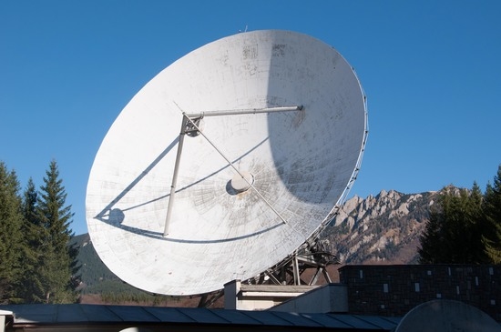
It was decided that a promising option is to retrofit the two existing C-band 32 m dish antennas, built and originally commissioned in 1976 and 1979, available in the National Space Communication Center in Cheia [2], situated 120 km north of Bucharest. A subsequent project [3] has expanded the study into assessing the status of the antennas, considered at a system level, and the main changes and improvements which should be implemented to design and build a ground-based SST radar, by using a quasi-monostatic configuration, where one antenna is transmitting and the other is receiving.
This paper describes the processes of design, implementation, and testing of the software and hardware blocks that make up the signal processor (SP) of the Cheia SST Radar. Section 1 presents similar signal processing systems from other radars. Section 2 contains the description of the Cheia Radar system and the purpose of its signal processor. Section 3 shows the results of the signal processor benchmarking. The paper ends with the Conclusions.
State of the Art
Modern radar systems are complex signal processing systems, built of subsystems and functional components which interact with each other via well-defined and often standardized interfaces. The signal processor is one of the most important components, as it is responsible for generating the output information used to detect targets. The signal processors of several space radars are detailed in the following paragraphs.
The Italian Bistatic Radar for LEO Tracking (BIRALET) uses a radio frequency (RF) transmitter located close to Calgari, Sardinia, with a fully steerable 7 m diameter parabolic antenna and up to 10 kW of output power [4,5]. The receiver is located 20 km away, close to San Basilio, Sardinia. This bistatic P-band (420 MHz) radar receives the target-scattered signal with a 64 m parabolic antenna and feeds it to an RF receiver block, which is intended for increasing the signal-to-noise ratio, changing the polarization from linear to circular, noise calibration, and selecting a 20 MHz bandwidth of the received signal with a bandpass filter. The next subsystem of the BIRALET radar is the new back-end that is capable of measuring also the slant range of the target, together with the Doppler shift. The new back-end uses a commercial field-programmable-gate-array (FPGA) software-defined-radio (SDR) ETTUS/NI USRP 2954R board. A second one is installed also in the transmitter subsystem, with the purpose of generating the digitally modulated signal to be transmitted. Both are synchronized with Global Positioning System (GPS) timing signals.
The received signal outputted by the RF receiver passes through an antenna focus selector and a power combiner, and then is fed to the USRP, where it is conditioned, down-converted to a frequency of 10 MHz, and digitized using 14 bits. The resulting in-phase and quadrature data are stored and processed on a workstation. This is using the ETUUS drivers, a LabView radar processing application, and a graphical user interface (GUI). The processing program generates the slant range and Doppler shift measurements of the detected target. A matched filter is used for correlating the well-known transmitted signal, with the unknown received signal, in order to detect the presence of the transmitted signal in the unknown signal. The matched filter is an optimal linear filter for maximizing the SNR in the presence of additive stochastic noise [4]. The transmitted waveform is a mixed signal composed of a frequency-modulated continuous wave (FMCW) signal (chirp), plus a CW tone, with an overall bandwidth of 5 MHz. The pulse repetition interval and pulse repetition frequency of the chirp assure the detection of targets at distances up to 3000 km. Because of the mixed transmitted signal, the system acts as a pulsed radar and also as a CW radar. The GUI contains the control panel, the status display, the measurements extractor, a spectrogram, and plots for range and Doppler for the received signal.
Another European sensor is ATLAS, a tracking radar system for space object detection situated in Portugal, operating in the C-band (5.56 GHz). It is a monostatic pulse radar with a maximum transmission power of 5 kW for tracking debris objects in LEO. The receiver stage is completely coherent, with completely digital detection and processing, with a bandwidth of 50 MHz, and with the capability to detect Doppler speeds up to 10.79 km/s [6]. The receiver includes an analog block that has the role of amplifying the input signals to the necessary digital input levels of the analog-to-digital conversion ADC board. The receiver begins with a low-noise amplifier. Next, there is a mixer to convert the input signal down to a 400 MHz intermediate frequency. The down-converted signal then passes through a bandpass filter and a digital variable gain amplifier, which is commanded by the controller board.
At last, the in-phase/quadrature detector demodulates the input to the baseband and outputs the I and Q parts of the echo signal. The data acquisition contains the acquisition board and a single-board computer. The acquisition is commanded by the controller board and is in charge of converting the I/Q signal parts to the digital domain, by using two 16-bit ADCs at a maximum sample frequency of 100 MS/s. The I/Q signal in the digital domain is fed to the computer (an MIO 2360 from Advantech headquarted in Taipei, Taiwan), which performs the required digital signal processing [6]. Communication between the acquisition board and the single-board computer is conducted via universal serial bus USB 3.0 (100 MS/s). A Fast/Slow mode buffer is available, acting as an alternative between increased sample resolution and increased sample rate.
The Spanish Space Surveillance and Tracking Radar (S3TSR) is an L-band (1400 MHz) radar, that works in a close monostatic configuration. Its architecture is scalable and is using electronically scanning arrays as transmitter and receiver antennas. The receiver uses direct Radio frequency undersampling technology. Each reception module, which is connected to four antenna array elements, employs four RF blocks for low noise amplification, filtering, and equalizing the signal, as well as a divider and switches for inserting a test signal in the four channels from a common input. The test signal is necessary for synchronization and calibration uses. The four augmented RF signals are fed to ADCs and the digital samples are used by a high-performance FPGA for digital down-conversion and beamforming. The receiver (Rx) array connects with the Processing and Control system inside the Rx Building. It includes the subsystem for the generation of all signals (transmitter Tx, test, and reference oscillator) required by the Rx antenna and the up to three Tx antennas. It also contains power amplifiers for the reference oscillator and test signal used by the Rx antenna, as well as passive splitting networks for both signals [7].
Signal and data processing capacities are offered by commercial high-end computers. They are integrated into the Processing and Control system. The signal processor is working on a single computer fitted with a PCIe board with fiber optic communication and a high-end FPGA. This board connects with the Rx array controlling and receiving the beamforming channel samples from the Reception Modules. It is responsible for the final stage of beamforming, concerning the integration of samples from the different antenna array rings. Samples for all Rx antenna patterns are fed to the processing software running on host processors through PCIe interfaces. The results of the signal processor are target detections that are fed to the Data Processor (DP). Initially, a correlation operation is applied by the DP for generating a sum plot of all detections for the same object at the same moment, obtained from processing the different Rx beams of the group assigned to the same Tx signal. The DP is responsible for the object tracking process, which starts with the results of the correlation operation. The tracking involves the identification of the group of plots that are generated by the passing of a space object through the field of view and the elimination of the false alarm plots generated by noise. For this scope, a recursive Least Square Error minimization algorithm is used, with an improvement of the track state vector in each iteration. After a trace is obtained, the set of related plot data, consisting of measured positions and radar cross-section estimations, is organized and sent to the connected users. The DP performs also a continuous recording and data dissemination task. Users connected to the radar through local or remote connections can ask for raw plots and track data from the recorded period. The signal and data processing algorithms are implemented in standard C/C++ language and executed on real-time Linux [7].
Another European space debris radar system is the German Tracking and Imaging Radar (TIRA)-Effelsberg bistatic system. It contains a 34 m fully computer-controlled parabolic antenna with a Cassegrain reflector, installed in Wachtberg, Germany. It can operate both in L-band (1.33 GHz) as a narrow-band monopulse fully coherent tracking radar and Ku-band (16.7 GHz) as a high-range resolution imaging radar [8]. The L-band transmitter of TIRA can transmit high-frequency pulses, usually from 1 to 2 MW peak power, in Right-Handed Circular Polarization (RHCP), while the Ku-band transmitter has a peak power of 13 kW. Working as a monostatic radar, the TIRA can detect objects with a diameter of 2 cm at a range of 1000 km. Moreover, when connected with the Effelsberg radio telescope of the Max-Planck-Institute of Radio Astronomy (MPIfR), comprising a parabolic dish with a diameter of 100 m located in Bad Münstereifel (Germany), used as a receiver, the size of detectable objects reaches 0.9 cm in diameter. The TIRA antenna can be turned at a radial speed of 24° per second and is protected inside a radome [9].
GESTRA (German Experimental Space Surveillance and Tracking Radar) is a quasi-monostatic scientific radar. This L-Band phased array radar is designed to monitor the low Earth orbit. It supports the German Space Situational Awareness Center to generate a catalog of orbital data for objects at altitudes between 300 and 3000 km. It was developed at the Fraunhofer Institute for high-frequency physics and radar techniques, based in Wachtberg, Germany [10]. The radar uses different antennas and shelters for transmitting and receiving. They are set up at a distance of about 100 m. Both antenna apertures consist of 256 active cavity-backed stacked patch antennas in a circular arrangement, whereby the transmitting radiators are excited with linear polarization, and the receiver’s radiator elements are designed with double polarization. The corresponding transmitter modules at the rear of the transmitting antenna are water-cooled. The receiving antenna uses the principle of digital beamforming. In addition, the antenna array can be rotated in any direction using a mechanical steering system [11].
GRAVES (Grand réseau adapté à la veille spatiale) is a bistatic radar system operated by the French Air Force in the VHF band at 143 MHz for orbit determination of artificial earth satellites at an altitude up to 1000 km. It is a space surveillance system developed by the French Aerospace Research Establishment (ONERA). It is a full electronic scanning bistatic continuous wave (CW) sensor, operating in very high frequency (VHF), using Doppler detection and digital beam forming reception technique. It transmits in up to three envelopes, at different elevations, for maximizing the number of detected targets. The transmission is implemented using a phased array and the reception is by a technique of digital beam forming [12]. The reception array comprises 100 antennas distributed over a metallic disc forming a ground-level surface. Each antenna is linked to an individual receiver whose signals are then digitized. The addition, in phase, of all the signals issuing from the reception antennas results in the creation of a vertical reception beam equivalent to that which would be created by a single antenna of the same size as the disc carrying the antennas.
With the signals issuing from each antenna being digitized, it is possible to assign to the signal from each antenna a specific phase shift. The choice of an adapted phase set allows the creation of a beam oriented in any direction, not simply the vertical. This technique of digital beam forming allows, given a real-time calculator of sufficient power, simultaneous observation in all directions potentially illuminated by the transmission. The detection of the satellites is then made possible with a Doppler technique by applying a Fourier transform to the sum signal. The transmitter site is located at Broye-Aubigney-Montseugny, and the receiver site is 364 km south of it at Revest-du-Bion. The radar was put into operation in 2005.
The ABISS project (Antenna BIstatic for Space Surveillance) is a ground-based surveillance radar demonstrator for European Space Agency. This European Space Surveillance radar breadboard is a bistatic system that is located on two separate sites in the northern part of France around Paris. This radar operates in L-band for the detection of space objects over a steerable Field of Regard (FoR) defined as 30° in azimuth by 25° in elevation oriented preferably to the south. One of the advantages of such a system is its operation with a continuous wave (CW) signal, which is easier for spectral management as it is strictly limited to the carrier frequency. The demonstrator has been designed on the basis of simulations of performances, as a radar which should have a reference detection range at 500 km for a reference target of 0 dBm² as radar cross section (RCS) for a revisit time of 10 s, meaning that the beam of the radar should revisit the same azimuth and elevation position within 10 s. These are the reference values that have been used in the power budget computation for the design of the system. The principle of the detection for such radar is only based on Doppler measurement; there is no evaluation of the distance of the target.
The transmitting system (Tx) is constituted of one antenna array of surface area 1.5 m² with 49 radiating elements, and 49 CW solid state power amplifiers, controlled in both phase and gain, associated with each radiating element. All electronic equipment for transmitting and control is in a shelter. The antenna array is set up under a radome on the roof oriented to the south. The positioner which hosts the antenna array can be steered through +/−90° in azimuth around a central position oriented in the south direction, and 0° to 90° in elevation. The receiving site (Rx) is within the ONERA center in Palaiseau. The antenna panel, with a surface area of 10.5 m² and 64 receiving antennas, is installed on the roof of an office building. The antenna array can be steered through +/−90° in azimuth around a central position oriented in the south direction, and it can be inclined from 0° to 90° in elevation. The receiving system is constituted of 64 analog front-end stages in one cabinet, four digital receivers with sixteen channels, and a cluster of ten computer servers to process the data.
The Field of Regard is completely covered with an average gain greater than 22 dB. The signal processing implemented in the radar consists of Doppler/acceleration measurements (i.e., speed estimation), detection, and monopulse compression for precise direction finding. As the Field of Regard is covered by 10 positions of the transmitting beam in 10 s, one second of signal is analyzed at each position. Consequently, the coherent integration time is 1 s. Thus, detections of objects that pass through the Field of Regard are characterized by Doppler traces versus time. The passage of one space object is signaled by a series of closely spaced radar plots. Each extracted plot contains all measurement parameters, namely azimuth, elevation, Doppler (speed), radial acceleration, and time of detection. Tracking of a previously detected target is realized with consecutive plots using the Track-While-Scan (TWS) method, which combines both search and track functions [13].
CASTR (Chilbolton Advanced Satellite Tracking Radar) is an S-band radar mounted on the 25 m steerable antenna at the Chilbolton Observatory in southern England. The dish is a fully steerable elevation over azimuth mount and is capable of tracking most satellites in LEO. A pulse repetition frequency (PRF) of 71.428 Hz, corresponding to a pulse repetition interval (PRI) of 14.0 ms and a maximum unambiguous range of 2100 km, was chosen so as to achieve alias-free range measurements for targets in low Earth orbit (LEO). Under these conditions, although the peak power is some 700 kW, the average transmitted power is only 25 W. The system’s polarizer was configured to transmit pulses of fixed, horizontal polarization, while the radar’s receivers simultaneously recorded both co-polar (horizontal, H) and cross-polar (vertical, V) target returns [14].
2. Materials and Methods
2.1. Radar System Description and Purpose of Radar Signal Processor (SP)
The Cheia Radar set-up has been finalized and has begun functional tests at the end of 2022. The ultimate set-up of the space radar installation is shown in Figure 1, containing: a transmitter (Tx), receivers (Rx), monitoring and control (M&C) server, and other subsystems.
The master oscillator (MO), the signal generator and the power amplifier (PA) are subsystems of the Tx. The transmitted signal and trigger pulses are generated by the low-noise signal generator, which is controlled by the M&C server and uses a reference signal from the MO. The generated signals are increased to the necessary level by the linear PA and then fed to the Tx antenna. A limited fraction of the transmitted signal is withdrawn in order to be employed as a local oscillator signal in the receiver [15].
The input signals are received by the Rx antenna, filtered, frequency translated/demodulated, and amplified into the Rx subsystem, to the level required for the best functioning of the analog-to-digital converter (ADC), that belongs to the signal processor (SP) [16].
The RF receiver (Rx) and the signal processor (SP) are the components of the Cheia radar’s receiver. The SP transfers the input signal into the frequency domain, time stamps, and analyzes it, using a constant false alarm rate method. The output is the space object’s range, relative speed and signal-to-noise ratio (SNR), which is used to evaluate the target’s radar cross-section. These output data are transferred to the M&C server. The M&C server is a computational system that controls the radar’s functioning through software process-based commands, implemented through the M&C software [17]. The hardware specifications and the functional parameters of the radar can be found in [18].
The purpose of the SP is to acquire analog data from the receiver, transform it into digital data, process it, detect space objects and describe their trajectory (distance to the object in time, speed of the object in time). A full system schematic is drawn in Figure 1 below where one can see top-level data exchange between the components of the radar.
The radar’s signal processor is a 4U Xeon server fitted with high-speed high-resolution ADC cards used in acquiring analog signals from the receiver and also fitted with a high-performance GPU used to accelerate digital data processing. The SP runs a Linux-based OS and on top of it a full suite of drivers topped with the FSM (finite state machine) of the SP, the top-most level software running on it.
2.2. The Hardware of the Signal Processor (SP)
In Table 1 below, one may see the main hardware components of the signal processor. The SP is a 4U server, with redundant power supply units and enough PCI-e slots to fit all components.
2.3. The Software of the Signal Processor (SP)
The SP runs a Linux-based OS on which a kill-safe multithreaded application runs (SPapp). The application handles the GPU using OpenCL API, the ADCs, the general-purpose IO board which also provides time tags (Ts) for timestamping the received signals, the TCP server which allows SP to be controlled remotely, the WDT, which restarts the SPapp if it becomes non-responsive and last, but not least, a service to reliably move acquired data towards the storage server.
In Figure 2, one may see the layered hardware (gray), and low-mid-high level software (up to down).
2.4. The Performance Requirements for the Signal Processor
The SP should assure real-time data processing of incoming data. Analog data are sampled at 100 MSa/s using 4 channels (two ADCs) of 16-bit; this results in a data rate of 100 M × 4 × 16 = 6.4 Gbps
As seen in Table 2 below, multiple scales for distances between 400 and 4000 km were used (and accordingly multiple settings for RF modulation and digital processing); this is due to the following reasons:
- It allows to keep a constant, relatively small RF bandwidth (2 MHz) which allows the receiver chain to keep noise under control (the noise is a product of bandwidth with spectral density). Constant bandwidth allows simpler receiver design, and one would prefer to modify the parameters of the receiving pipeline, in software (digital domain) in the SP, as opposed to temper with the analog part in the receiver. The complex receiver means complex tuning across different frequencies (we use frequency modulation).
- The power scattered by the target (the echo signal) decreases with a power of 4 of distance, so the further away the target is, the much worse would be for the SNR. This requires a much better noise cancellation algorithm, which requires a larger FFT, which requires a longer signal in time (continuous emission over larger distances requires a longer time-duration of the signal due to longer round-trip time).
There is only one performance requirement, and it is for the processing of an acquired wave, depending on the processing time of this required acquisition, as can be seen in Table 2:

Table 2.
Radar scales for different ranges.
| Scale Number | Description (Range) | Range (km) | Trigger Period (ms) | Acquired Wave Size (Samples) | Maximum Processing Time (ms) |
|---|---|---|---|---|---|
| 1 | Close | <400 | 40 | 256 k | 40 |
| 2 | Mid-close | <900 | 100 | 512 k | 100 |
| 3 | Mid-far | <1800 | 250 | 1 M | 186 |
| 4 | Far | <3900 | 500 | 2 M | 290 |
2.5. The FSM of the Main Signal Processor
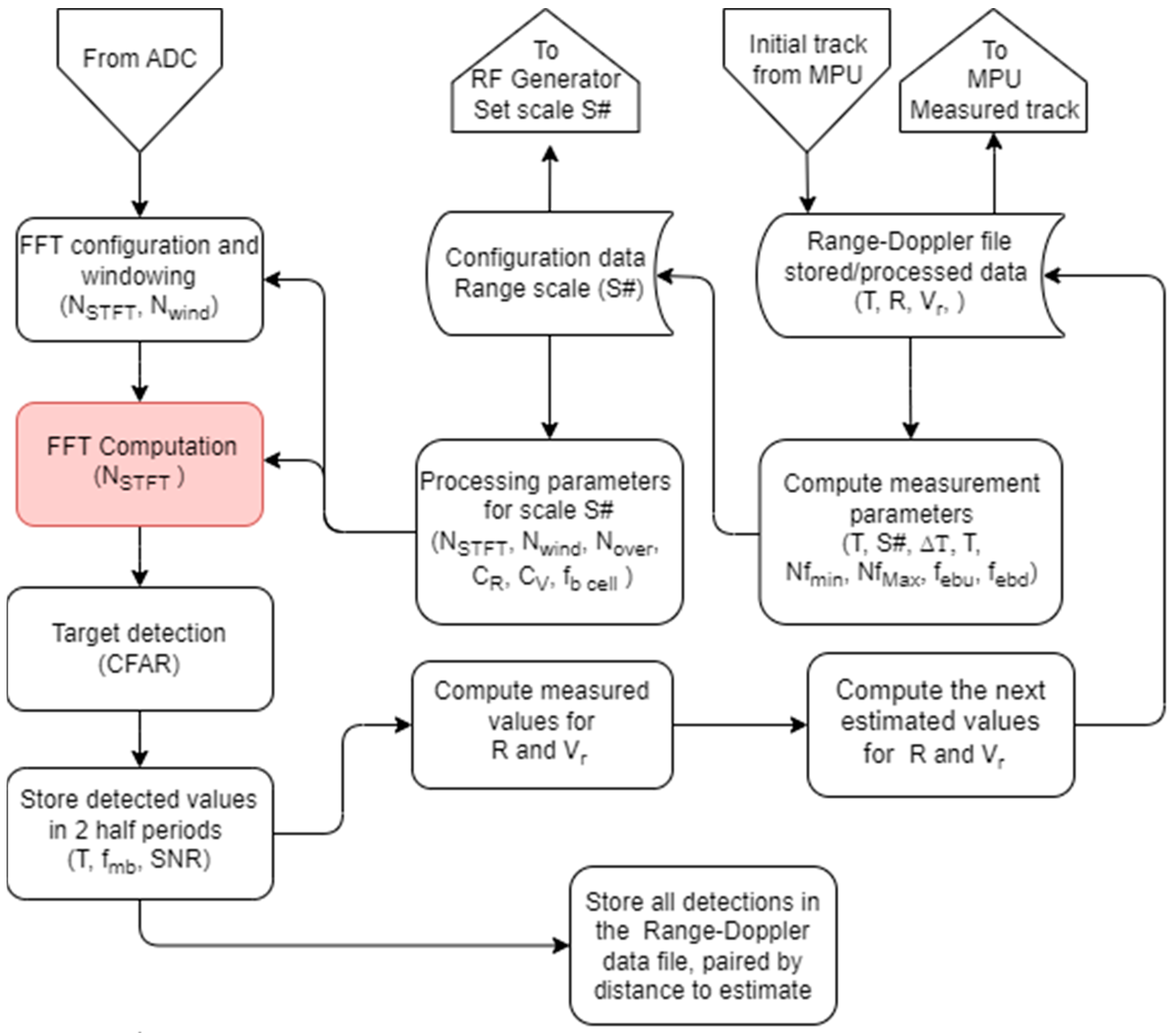
The signal processor acquires data from the receiver, processes it, and logs data and results. In addition to this functionality, it also allows for fine-tuning of its 40+ parameters. Its finite state machine diagram is visible in Figure 3.
2.6. The Modifiable Parameters of the Signal Processor
The behavior of the signal processor may be altered by changing the values of several parameters. A list of such parameters is presented in Table 3.
2.7. Other Considerations Regarding the System Reliability and Performance
A few techniques were used to improve the quality of the signal processor:
- Creating and using a simulator to play back the data without the need for a real space target;
- Using references instead of memory pointers;
- Using the software Watchdog Timer;
- Intercepting all OS signals sent to the application, to graciously close used resources in case of system errors/crashes;
- Auto-restart the app with the last auto-saved settings and commands received from the M&C system;
- All data processing operations were tested against Octave implementation to check for precision loss;
- All computation was performed in double precision (fp64).
2.8. Software Inside the Signal Processor
2.8.1. Software Class Diagram
The software for the SP (illustrated in the diagram from Figure 4) is split into various components:
- Components that assure communication with the outside systems (range setter, M&C thread, Message Center, Message);
- Components that assure communication between SP’s components (SWave, ConcurrentQueue);
- Components that assure data processing (CFAR, ABfilter, FFT, Windowing);
- Components that assure data acquisition (Data Generator, Config Sink);
- Components that enable data output (File Move Thread, File Copy Thread, BB*file);
- Components that enable testing;
- Components that assure reliable behavior in case of errors (WatchDog Thread, CPUusage Thread);
- Top-level component of MSP (Main Signal Processor which uses all the other components).
Regarding the data flow, the SP was fitted with an inheritance class hierarchy so that data may come and go from either hardware or software (simulator) source/sink.
2.8.2. Digital Processing Operations
The intensive digital processing operations performed by the SP are:
- DEC (decimation using a custom factor 5);
- FFT (1D complex-to-complex conversion of time-domain to frequency-domain data);
- ABS (absolute value of complex numbers);
- CFAR (applying a constant false alarm rate detection algorithm);
- ABF (alpha-beta filter, for predictive range and radial speed).
DEC (Decimation)
Two versions of decimation with factor F were tested:
- Decimation by sampling: output sample is one of the F consecutive samples;
- Decimation by averaging: output sample is the average of F consecutive samples.
The DEC computation since it was in O(N), was more efficient to be performed in parallel in the CPU using OpenMP.
FFT (Fast Fourier Transform)
The FFT is a faster way (as opposed to DFT) of creating a frequency representation of a periodic signal. Initially discovered by Gauss around the same period of time as Fourier discovered the Fourier transform (1800s), it was rediscovered in the 1960s in the context of Soviet Union-US meetings for differentiating underground nuclear tests from the earthquakes, with the higher purpose of the worldwide partial nuclear test ban. In 1963, it effectively reduced the time needed to process an incoming seismograph data stream of an analyzed event, from 3 years to 30 min (that is the difference between O(NlogN) DFT’s complexity of O(N2)). FFT takes advantage of similarities found in the sinewaves that have the frequencies multiple of the fundamental frequency, which allowed for far fewer multiplications than in DFT. In both cases, FFT and DFT, the more samples the time-signal contains, the more frequency bins we obtain; this is why we thought of using a larger FFT transform to obtain a better determination of frequency components in the radar’s received signal (it effectively reduces noise in that bin and allows for weaker signals to be detected with a frequency-based CFAR algorithm)
We used an OpenCL implementation of O (5*N*log(N)) similar to the Cooley–Tuckey version. In addition, an extra layer of cache was developed (the first run takes more, subsequent ones take less time); in this software cache, we saved the plans (mainly the fiddle factors) and GPU memory allocation buffers and just-in-time compiled programs, for common sizes, so a warm-up phase is executed at application start-up to improved performance on subsequent runs.
ABS (Absolute Value)
The ABS is a straightforward absolute value computation of complex numbers. This is also an O(N) complexity so unless other advantages are drawn running in the GPU, it will be run in the CPU. Since the log is applied to extract SNR, at some point, the sqrt may be skipped (let us note that operation, as absm) by using a factor of 2 afterward (log ab = b log a).
Assuming , a complex number, the , and therefore the .
CFAR (Constant False-Alarm Rate Algorithm)
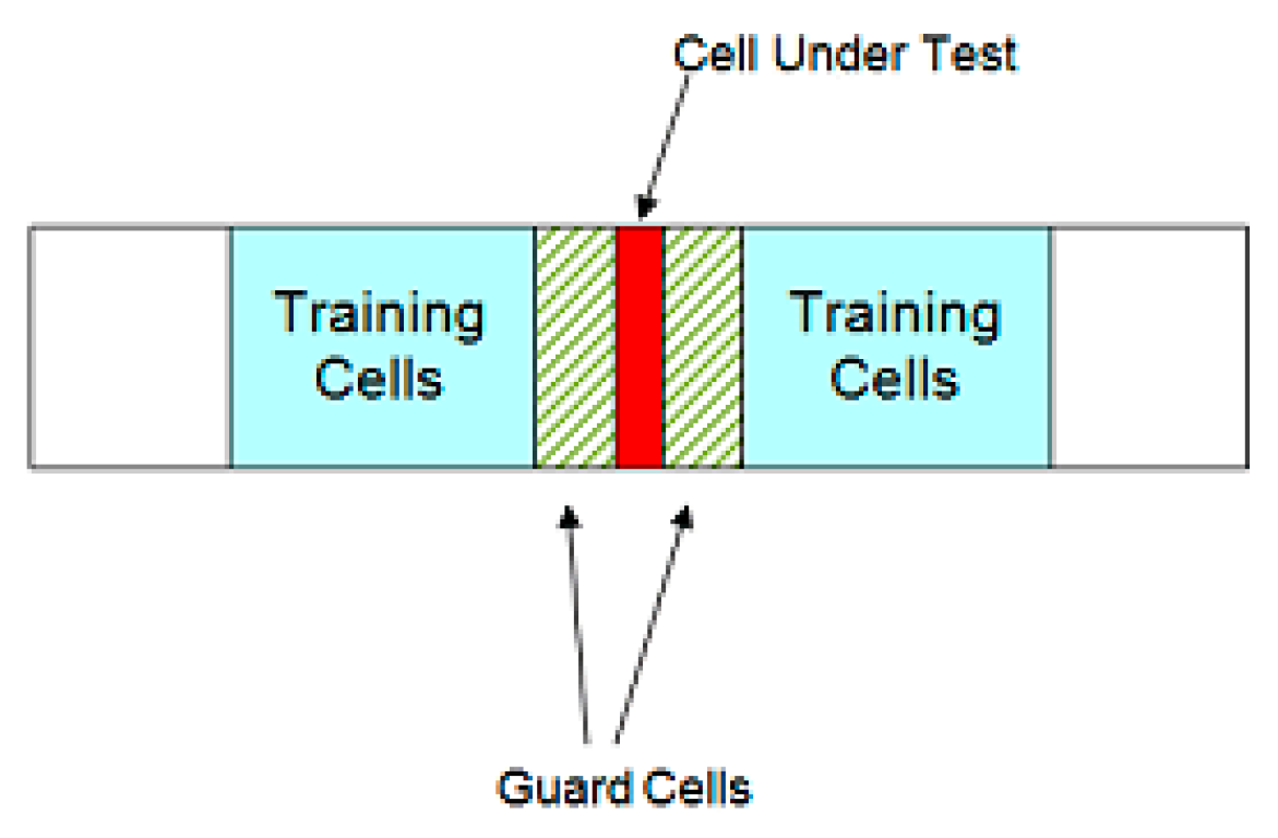
The CFAR algorithm uses a moving window to detect peaks in a wave. It can be used in both time-domain and frequency-domain, to detect local peaks. Local peaks are selected using an average of left training cells and right training cells on one side and the other of the peak-candidate value (cell under test). To avoid false peak detections near an actual peak, usually one uses “guard” samples between the candidate value and the left/right samples, as depicted in Figure 5 and Figure 6.
An avg of left-side training cells is computed AVGL = sum (left_samples)/num_left_samples.
An avg of right-side training cells is computed AVGR = sum (right_samples)/num_left_samples.
There are three versions of threshold calculation, usually used to compute the threshold, depending on how much weight the two halves (left and right) have:
- CA-CFAR (Cell Averaging), Threshold = (AVGL + AVGR)/2;
- GO-CFAR (Greatest Of), Threshold = max(AVGL, AVGR);
- LO-CFAR (Least Of), Threshold = min(AVGL, AVGR).
ABF (Alpha-Beta filter)
The alpha-beta filter was fitted with multiple simulated trajectories to see its behavior when trying to predict the next range or radial speed. An example of the trajectory that was tested may be found in Section 3.1.2 below.
2.9. Graphical User Interface of Signal Processor (SP gui)
While the SP may be used without a graphical user interface (gui), during test phases (where various hardware or satellites to be tracked may be unavailable) one needs to be able to simulate the SP’s activity. For this purpose, a simulator module was developed (which is based on real acquisitions made previously). The graphical interface can connect itself either to the real SP or to the simulated SP and provides an insight into the data acquisition and processing (configuration, status, and data) for either a real-time run (“real-time mode”) or a previous run (“analysis mode”). In addition, the gui allows issuing commands as if they were coming from the M&C system, to allow SP’s testing even when M&C was in development or upgrade.
In real-time mode, all runtime parameters, configuration, and limited data of the SP are monitored while the acquisition is performed.
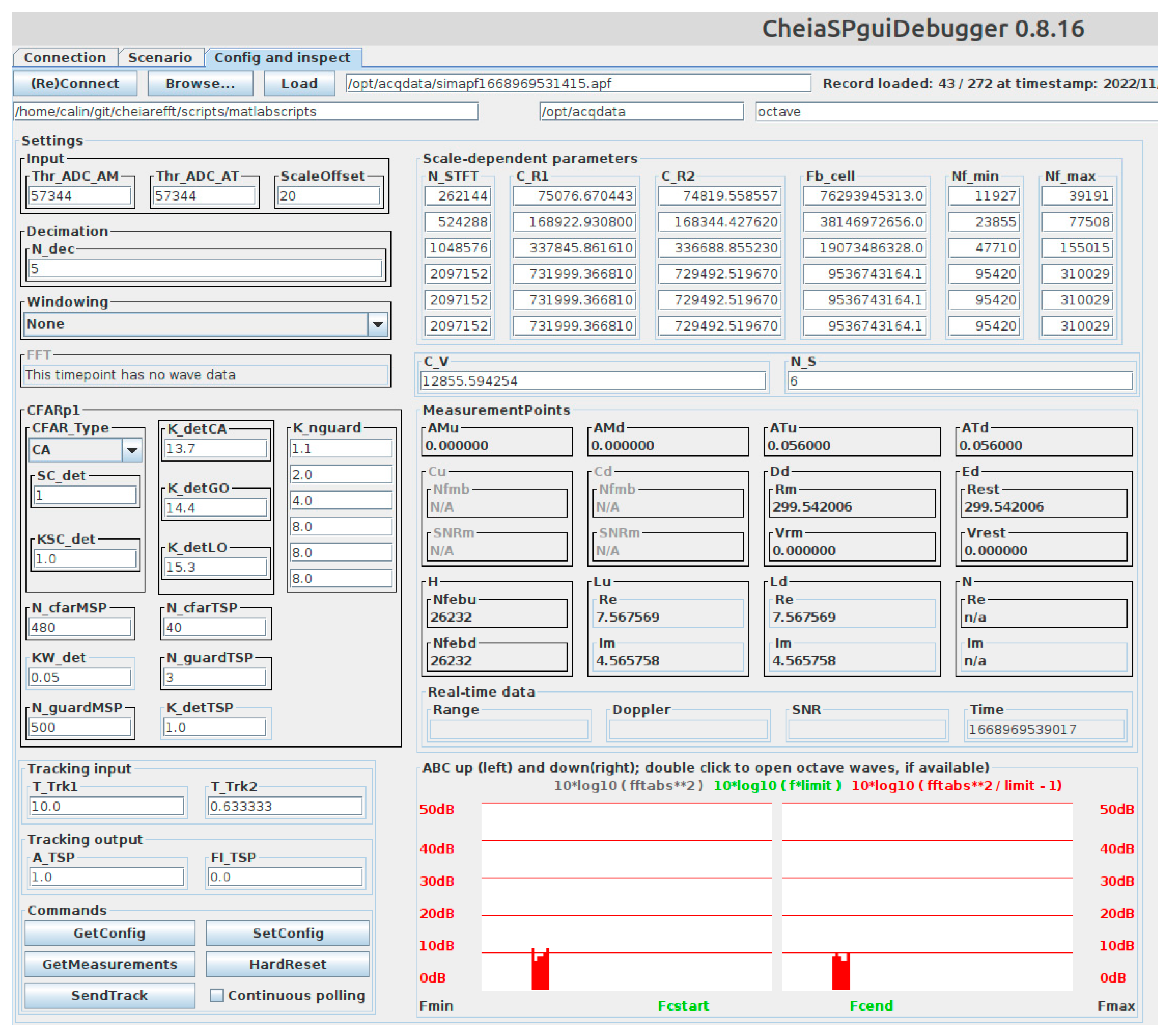
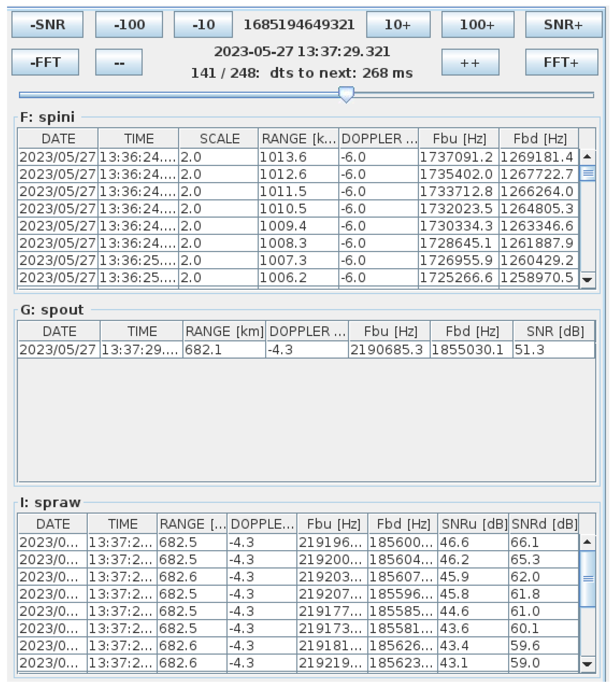
In analysis mode, the previously captured data (and acquisition settings), may be visually inspected and played back frame by frame to see if the SP works as expected. If the captured data need to be detailed, an Octave script will be invoked from the gui, to parse the large debugging data. Figure 7 shows a caption from the SP gui application, while in real-time mode with real-time data disabled, Figure 8 shows the SP gui application in analysis mode, and Figure 9 shows the Octave script’s figure display for an acquisition that produced valid data.
3. Results of the Signal Processor Benchmarking
The results of SP processing may be split in two categories:
- quality of computation
- performance of computation
The performance was evaluated on a Xeon W-3223 CPU @ 3.50 GHz (8C/16T) with 3 × 32 GB of DDR4 and an Nvidia GPU Tesla V100s-32 GB with CUDA 11.0 and Driver Version: 450.80.02 on Linux 5.4.0-89.
3.1. Measuring the Quality of Digital Processing
3.1.1. Measuring the Quality of the FFT
We tested our CPU and GPU-accelerated version against the Octave implementation, then we calculated the sum of squared differences for various FFT sizes. The results are summarized in Table 4.
3.1.2. Measuring the Quality of the ABF
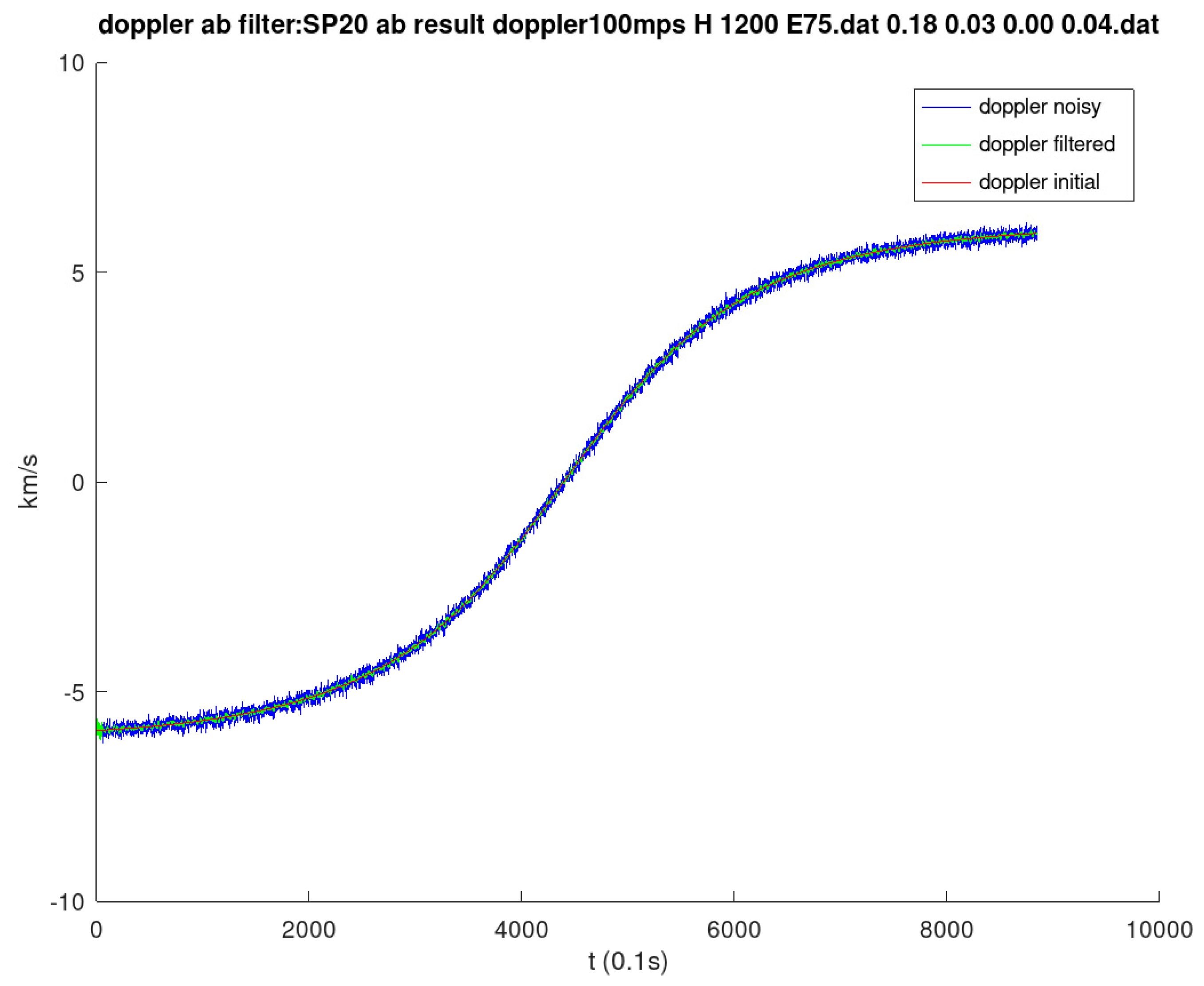
We first generated simulated range and Doppler tracks (22 scenarios, generated by experts in space trajectories), added noise then filtered them to check how well the alpha-beta filter works. Then we swept all values from 0.01 to 0.99 step 0.01 for both alpha and beta (in total 10,000 combinations) for all range or Doppler scenarios. The best (least RMS between filtered and initial values) was selected out of them and transformed into drawings to allow visual checks. Such a scenario is depicted in Figure 10, Figure 11, Figure 12 and Figure 13 below, where alpha is set to 0.26 and beta to 0.03. We plotted for each case, the filtered–initial and the noisy–initial so we can compare them visually. Figure 10 and Figure 11 are for range, Figure 12 and Figure 13 for radial speed (but with alpha of 0.18 and beta of 0.03).
3.1.3. Checking the Quality of CFAR Algorithms
We generated scenarios with sinewaves of 1 MHz and 2.9 MHz (expected minimum and maximum values) and we swept various ranges of guard cells, averaging window size, and CFAR factor. An example of such a scenario is in Figure 14 below. The algorithms were thus validated.
3.2. Measuring the Performance of Digital Processing
The main performance-intensive operations for the longest data acquisition are listed in Table 5 below. The operation of WIN_FFT_ABS_CFAR does all these ops in a chained manner (without transfers to/from GPU memory while between the ops). The difference between chained operations and non-chained operations is quite large. For example, the WIN_FFT_ABS_CFAR if chained, can be performed in 16 ms whereas when WIN + FFT + ABS + CFAR are performed independently, one will only finish the operations in 61 ms; the advantage of having the operations independently is the ability to save intermediate results for later investigations. This was mitigated in the end, by creating a buffer in the GPU memory where only one such intermediate result may be saved, per each WIN_FFT_ABS_CFAR operation (usually it was used for the absolute value output).
3.3. Measuring the Network Performance
Multiple software commands are available for using the signal processor (SP). The SP has two hardware network interfaces:
- A NIC with 1 Gbps is used for command and control (an SP server listens on a TCP port);
- A NIC with 10 Gbps is used for large data transfer/long-term storage (over Samba/CIFS protocol).
3.3.1. Measuring the Network Performance (Commands)
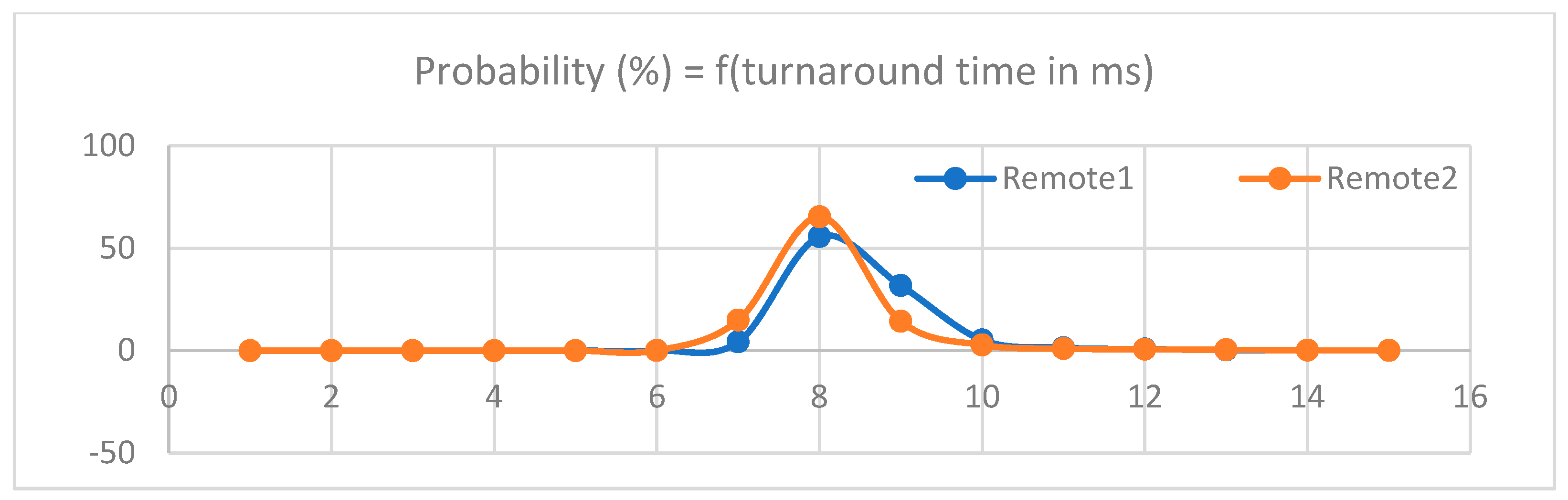
To test network latency, we chose the get_status command, which returns a JSON-based string over a TCP connection with data about the state of the SP. Usually, the command contains 20 bytes whereas the answer usually contains 166 Bytes. We benchmarked the command in the local scenario (client and server are on the same machine, the signal processor) and remote scenarios (the server is on the signal processor machine and the client is around 111 km afar). The turnaround time is measured from the moment the client sends the command until the client receives the answer from the SP’s server. The results are listed in Table 6. The spread (histogram) of the turnaround time is plotted in Figure 15 below. It shows that 8 ms is the most probable turnaround time.
3.3.2. Measuring the Network Performance (Large Data)
As previously stated, the 10 Gbps network interface card is used to transfer large data from the SP to the storage server, for future analysis. The SP functions as follows:
- SP is powered-up and its main software starts;
- SP runs self-tests (speed and accuracy tests) to ensure correct operation;
- SP warms-up (builds a data cache with most common operations and compiles all the OpenCL programs to be run on GPU, to save time when executing a real-life measurement);
- The SP receives a command from the Monitor & Control (M&C) system, where the expected track during expected timestamps (beginning (T), ending and a few timestamps in the middle) are given;
- The SP arms itself, interpolates the track (with position and time data) at 100 ms;
- At about T-4 s a short system check is performed to make sure SP module work as expected; in case of problems various misbehaving subsystems are restarted;
- At about T-1 s, data acquisition starts (using a parallel software thread), but data are dropped until T time occurs;
- Data are acquired every 100 ms and are pushed into data queues. A separate software thread starts processing it. The SP switches from debug mode (acquiring and storing large data wave from ADC output, decimated output, FFT output, and CFAR output) to fast mode (only one debug wave is saved, usually the FFT output) dynamically depending on the time budget;
- When the acquisition end occurs, SP stops data acquisition and starts transferring output and debug data into the storage server; simultaneously the M&C system polls it to check the status and retrieve the results.
The data generated for debugging purposes (or later analysis) may be quite large, so the faster 10 Gbps link was used to transfer it to the storage server. In Table 7, we present the results of such measurements of data transfer (the data contained about 6 GB of waves: DEC output, ABS output, CFAR output, CFAR threshold, and CFAR output; all waves were 8 MB long and were acquired at a rate of 2× per every 100 ms, therefore would amount for about 8 s of processed data).
The results are somewhat expectable since the data storage is using SSD storage memory for source and large HDDs in RAID5 configuration, as destination.
3.4. Performance Impact of Hardware and Digital Processing
The ABISS radar uses two phased array antennas and low transmitted power but is intended only for re-entry (altitude < 200 km) and objects of size higher than 2 m.
The Cheia Radar is designed for LEO tracking (200–2000 km altitude), having a potential detection capability of 5 cm at 1000 km. The Cheia Radar makes use of 2 decommissioned Cassegrain antennas, previously used for satellite communication, and exhibits detection capabilities similar to TIRA but, due to a special signal processing needs to transmit only a fraction of TIRA’s transmitting power.
Although the Main Signal Processor is not the only contributor to these results, together with a good choice of frequency generator and a custom implementation of the analog receiver, they enable the radar to perform side by side with the BIRALET system, as seen in Table 8.
4. Discussion and Conclusions
In radars, there is always a tradeoff between the transmitted power and the minimum RCS of the detectable target, for a given range or between the transmitted power and the maximum range, for a given RCS of the target.
The limit is always determined by the target’s signal-to-noise ratio (SNR) at the input of the target’s extractor. The article shows that this limit can be drastically reduced by signal processing. For example, assuming a Swerling 5 radar case model, to obtain a detection probability of 0.9 and a false alarm probability of 10−6, an SNR of 13.2 dB is required at the input of the target detector. The noise power is proportional to the receiver bandwidth, which is in the ranges of MHz to tens of MHz, for a regular time processing radar. A frequency processing radar, using a 1 M sample FFT would then generate a bank of 1 million filters with a bandwidth of Hz to tens of Hz each. In each of those filters, the noise power will be 60 dB less, due to the 60 dB reduction of the bandwidth, while the signal power will be contained by a single or a reduced number of filters. If the total power of the received signal is contained within one filter bandwidth, the SNR at the input of a target detector analyzing the output of each filter is reduced by 60 dB, thus requiring an SNR of −47 dB (60 dB less) at the output of the receiver. Some additional digital processing losses of 2 dB should be also considered.
Reducing the required SNR at the output of the receiver translates in significantly greater sensitivity and/or reduced transmitted power.
Reduced transmitted power translates into smaller costs of operation, reduced power requirements, and consequently a reduced ecological fingerprint.
This reduction comes with the cost of increased complexity of the signal processing as well as with some restrictions that have to be well understood. For the space radars, operating at very large ranges, this kind of processing is particularly suitable.
The advances in signal processing-related devices, especially high dynamic range ADCs and high-speed GPUs or FPGAs will make this kind of processing more and more common once its advantages are understood and mastered.
Future research directions include further reducing the required SNR by increasing the dynamic range of the ADC and designing new types of probing signals and processing algorithms to overcome the received signal length limitations.
The improvements in increasing the dynamic range of the ADC need to be studied and tested as soon as ADCs having more than 16 bits will be available in the video domain.
The design of new types of probing signals and processing algorithms have to be studied for implementation in shorter-range radars that are limited by the short time length of the received signal and by the reduced GPU and FPGA processing speed.
In conclusion, this paper presents in detail, the design, implementation, and testing of the software and hardware elements that compose the signal processor used by the Cheia Space radar for the acquisition and tracking of the targets. The first part of this work contains a review of the state of the art, with similar signal processing systems from other radars. Next, the architecture of the signal processor is explained, together with its state diagram and parameters. Also, a comparison is shown between the outputs of the signal processor and the results obtained with benchmark processing algorithms.
The novel contributions of the presented architecture come from the uncommonly large FFT length (up to 4096 k points) that is employed, allowing the tracking of targets with low RCS, in the context of Tx power lower than what other space radars are emitting [18]. The usage of frequency processing, using large-sized FFTs, allows a significant reduction of transmission power requirements and consequently a reduced ecological fingerprint in radars, to a degree similar to the implementation of the chirp pulse instead of the unmodulated pulse. The strong points of the Cheia receiver are also illustrated by the comparison with the BIRALET bistatic radar, which shows the higher optimization and sensitivity of the Romanian design, due mostly to the superior signal processor.
As of the first quarter of 2023, the Cheia Radar is completely implemented on-site and is undergoing calibration, functional testing, and validation procedures according to EUSST requirements.
Author Contributions
Conceptualization, C.B. and L.I.; data curation, C.B. and L.I.; formal analysis, L.I. and C.B.; investigation, L.I., A.R.-C. and C.B.; methodology, L.I. and A.R.-C.; project administration, L.I. and A.R.-C.; software, C.B. and L.I.; supervision, L.I. and A.R.-C.; validation, L.I.; visualization, L.I. and C.B.; writing—original draft, C.B. and A.R.-C.; writing—review and editing, C.B., A.R.-C. and L.I. All authors have read and agreed to the published version of the manuscript.
Funding
The research and development activities described in this paper were carried out within a series of three contracts financed by the European Space Agency (ESA) and awarded to a consortium led by RARTEL S.A., Bucharest, Romania: SSA for Romania, Contract No. 4000108671/13/D/MRP; SSA P3-SST-IV-CHEIA PHASE 1; SSA P3-SST-V-CHEIA PHASE 2.
Data Availability Statement
The data presented in this study are available on request from the corresponding author. The data are not publicly available due to the clauses of the previously-mentioned contracts.
Acknowledgments
We would like to thank RARTEL’s, Silicon Acuity SRL’s, and AdHoc Telecom Solution’s employees for their hard work in making the project, and therefore, this paper, possible. In addition, we would like to thank the Politehnica University of Bucharest for supporting us by funding various taxes for conferences and journals, therefore making our scientific journey, possible.
Conflicts of Interest
The authors declare no conflict of interest. The funders had no role in the writing of the manuscript or in the decision to publish the results.
References
- EUSST Consortium. ESA Safeguarding European Space Infrastructure. Available online: https://www.eusst.eu/about-us/ (accessed on 2 July 2022).
- Societatea Naţională de Radiocomunicaţii S.A. (RADIOCOM), Centrul de Comunicaţii Prin Satelit CHEIA. Available online: https://www.radiocom.ro/Materiale/Cheia/Centrul%20de%20Comunicatii%20prin%20Satelit%20CHEIA.pdf (accessed on 2 February 2023).
- Ionescu, I.; Scagnoli, R.; Istriteanu, D.; Turcu, V. Cheia Antennas Retrofit to a Space Tracking Radar. In Proceedings of the European Space Agency 1st NEO and Debris Detection Conference NEOSST1, Darmstadt, Germany, 22–24 January 2019; Available online: https://conference.sdo.esoc.esa.int/proceedings/neosst1/paper/415/NEOSST1-paper415.pdf (accessed on 20 February 2023).
- Schirru, L.; Pisanu, T.; Podda, A. The Ad Hoc Back-End of the BIRALET Radar to Measure Slant-Range and Doppler Shift of Resident Space Objects. Electronics 2021, 10, 577. [Google Scholar] [CrossRef]
- Muntoni, G.; Schirru, L.; Montisci, G.; Pisanu, T.; Valente, G.; Ortu, P.; Concu, R.; Melis, A.; Urru, E.; Saba, A.; et al. A Space Debris-Dedicated Channel for the P-Band Receiver of the Sardinia Radio Telescope: A Detailed Description and Characterization. IEEE Antennas Propag. Mag. 2020, 62, 45–57. [Google Scholar] [CrossRef]
- Pandeirada, J.; Bergano, M.; Neves, J.; Marques, P.; Barbosa, D.; Coelho, B.; Ribeiro, V. Development of the First Portuguese Radar Tracking Sensor for Space Debris. Signals 2021, 2, 122–137. [Google Scholar] [CrossRef]
- Casado Gómez, R.; Martínez-Villa Salmerón, J.; Besso, P.; Alessandrini, M.; Pinna, G.; Prada, M. Initial operations of the breakthrough Spanish Space Surveillance and Tracking Radar (S3TSR) in the European context. In Proceedings of the 1st NEO and Debris Detection Conference, Darmstadt, Germany, 22–24 January 2019; Available online: https://conference.sdo.esoc.esa.int/proceedings/neosst1/pap`er/479 (accessed on 20 February 2023).
- Muntoni, G.; Montisci, G.; Pisanu, T.; Andronico, P.; Valente, G. Crowded Space: A Review on Radar Measurements for Space Debris Monitoring and Tracking. Appl. Sci. 2021, 11, 1364. [Google Scholar] [CrossRef]
- Space Observation Radar TIRA [Online]. Available online: https://www.fhr.fraunhofer.de/en/the-institute/technical-equipment/Space-observation-radar-TIRA.html (accessed on 27 May 2023).
- GESTRA Space Radar Passes Its First Test, [Online]. Available online: https://www.dlr.de/en/latest/news/2019/04/20191129_latest-radar-technology (accessed on 27 May 2023).
- GESTRA [Online]. Available online: https://www.radartutorial.eu/19.kartei/02.surv/karte075.en.html (accessed on 27 May 2023).
- Michal, T.; Eglizeaud, J.P.; Bouchard, J. GRAVES: The new French System for Space Surveillance. In Proceedings of the Fourth European Conference on Space Debris, Darmstadt, Germany, 18–20 April 2005. [Google Scholar]
- Saillant, S.; Flécheux, M.; Mourot, Y. Detection of ExoMars launcher during its passage over Europe with Space Surveillance radar breadboard. Adv. Sci. Technol. Eng. Syst. J. 2018, 3, 99–105. [Google Scholar] [CrossRef]
- Ladd, D.; Reeves, R.; Rumi, E.; Trethewey, M.; Fortescue, M.; Appleby, G.; Wilkinson, M.; Sherwood, R.; Ash, A.; Cooper, C.; et al. Technical Description of a Novel Sensor Network Architecture and Results of Radar and Optical Sensors contributing to a UK Cueing Experiment. In Proceedings of the Advanced Maui Optical and Space Surveillance (AMOS) Technologies Conference, Maui, HI, USA, 19–22 September 2017. [Google Scholar]
- Tatomirescu, A.; Rusu-Casandra, A. C-Band FMCW RADAR Receiver Architecture for Space Debris Observation. In Proceedings of the 2022 14th International Conference on Communications (COMM), Bucharest, Romania, 16–18 June 2022; pp. 1–5. [Google Scholar] [CrossRef]
- Bira, C.; Rusu-Casandra, A. Dataset of Spatial Objects Acquired Using Romania’s First Ground-Based Space Tracking Radar. In Proceedings of the 14th International Conference on Communications COMM 2022, Bucharest, Romania, 16–18 June 2022. [Google Scholar] [CrossRef]
- Tramandan, I.; Rusu-Casandra, A. A Real-Time Monitoring and Command System for the Cheia Space Surveillance and Tracking Radar. In Proceedings of the 2022 International Symposium on Electronics and Telecommunications (ISETC), Timisoara, Romania, 10–11 November 2022; pp. 1–5. [Google Scholar] [CrossRef]
- Ionescu, L.; Rusu-Casandra, A.; Bira, C.; Tatomirescu, A.; Tramandan, I.; Scagnoli, R.; Istriteanu, D.; Popa, A.E. Development of the Romanian Radar Sensor for Space Surveillance and Tracking Activities. Sensors 2022, 22, 3546. [Google Scholar] [CrossRef] [PubMed]
- MathWorks Help Center, Constant False Alarm Rate (CFAR) Detection [Online]. Available online: https://nl.mathworks.com/help/phased/ug/constant-false-alarm-rate-cfar-detection.html (accessed on 20 February 2023).
- Constant False Alarm Rate (CFAR) [Online]. Available online: https://www.wikiwand.com/en/Constant_false_alarm_rate (accessed on 20 February 2023).
- USRP-2954 Specifications [Online]. Available online: https://www.ni.com/docs/en-US/bundle/usrp-2954-specs/page/specs.html (accessed on 27 May 2023).
Figure 1.
System schematic of the radar. In the center—the signal processor (blue rectangle). The antennas transmit the signal and receive the echo from the space object, the master oscillator provides a very reliable, very precise external clock for the SP’s ADCs, the monitoring and control (M&C) server offers the user interface and manages the system, and the storage server stores the acquired data. Red arrows denote analogue signals, green arrows denote digital signals.

Figure 2.
Signal processor inner schematic. Top is hardware and towards the bottom, software of increasing abstractness and complexity. The dark-grey components are hardware, the red components are low-latency threads, the blue components are GPU-enabled parallel processing components, the yellow components are the same parallel-processing components, but optimized for CPU. The dark green components are the middleware used to improve the performance of the GPU tasks, and the light green are the glue-logic or additional components without specific low-latency or high-performance requirements. The light-grey component is the finite state machine that commands and controls every other software subsystem in the Signal Processor.

Figure 3.
The FSM of the signal processor. Digital data flows inside from the ADCs, and they are processed by decimation and windowing, FFT, absolute value, and CFAR. The FFT processing is highlighted in red, as this has a very large size, quite unusual in a radar system.
Figure 3.
The FSM of the signal processor. Digital data flows inside from the ADCs, and they are processed by decimation and windowing, FFT, absolute value, and CFAR. The FFT processing is highlighted in red, as this has a very large size, quite unusual in a radar system.

Figure 4.
The class diagram for the SP software. MSP is assembled by composition using objects of all the classes above (denoted with blue arrows).
Figure 4.
The class diagram for the SP software. MSP is assembled by composition using objects of all the classes above (denoted with blue arrows).

Figure 5.
The CFAR moving window—choice of cells. Reprinted/adapted with permission from Ref. [19]. © 1994–2023 The MathWorks, Inc.
Figure 5.
The CFAR moving window—choice of cells. Reprinted/adapted with permission from Ref. [19]. © 1994–2023 The MathWorks, Inc.

Figure 6.
The CFAR moving window—choice of peak [20]. Usually, the threshold is multiplied with a factor, to obtain the actual threshold that will be utilized in peak detection. Credit: Nanoatzin License: CC BY-SA 3.0.
Figure 6.
The CFAR moving window—choice of peak [20]. Usually, the threshold is multiplied with a factor, to obtain the actual threshold that will be utilized in peak detection. Credit: Nanoatzin License: CC BY-SA 3.0.

Figure 7.
SP gui application when in real-time mode. The top-left part of the GUI is populated with configuration data; the bottom and middle part contains real-time data (during acquisition); “**”expresses pow function of 2 (squared).
Figure 7.
SP gui application when in real-time mode. The top-left part of the GUI is populated with configuration data; the bottom and middle part contains real-time data (during acquisition); “**”expresses pow function of 2 (squared).

Figure 8.
Extract of SP gui application while in analysis mode, with test data. The tables summarize the produced data (input track, raw data, filtered data, data seen and parsed by the CFAR engine, etc.). The top part contains a navigation menu, used to go through the records of the previously acquired data: the navigation may be made 1-by-1, 10-by-10, 100-by-100, or from/to the next/previous frame that contains a full FFT output wave or SNR data over a predetermined value.

Figure 9.
Octave script output. The SP GUI was running in analysis mode, and the user requested a detailed view of the monitored frequency spectrum. The top part contains the 0–4 MHz monitored spectrum: with blue, it is the output of the FFT as computed by SP, with gray is the output of the FFT computed by Octave, based on the raw data from the SP, and with green is the threshold of the CFAR algorithm. The bottom part contains the same 0–4 MHz spectrum but only with the peaks that exceeded the CFAR threshold.

Figure 10.
Example with a scenario for the alpha–beta filtering. The range (distance to the object, in km) decreases until it is as close as possible to the radar, then it goes further away.
Figure 10.
Example with a scenario for the alpha–beta filtering. The range (distance to the object, in km) decreases until it is as close as possible to the radar, then it goes further away.

Figure 11.
Example with a scenario for the alpha–beta filtering. The differences in filtered–initial values (green) are compared to the differences noisy–initial values, in time. The result is as expected since the green wave has a smaller spread than the blue one.
Figure 11.
Example with a scenario for the alpha–beta filtering. The differences in filtered–initial values (green) are compared to the differences noisy–initial values, in time. The result is as expected since the green wave has a smaller spread than the blue one.

Figure 12.
Example with a scenario for the alpha–beta filtering of radial speed. The Doppler (radial speed in fact) shows that the object approaches the radar up until some point in time, and then it goes further away.
Figure 12.
Example with a scenario for the alpha–beta filtering of radial speed. The Doppler (radial speed in fact) shows that the object approaches the radar up until some point in time, and then it goes further away.

Figure 13.
Example with a scenario for the alpha–beta filtering of radial speed. The differences in filtered–initial values (green) are compared to the differences noisy–initial values, in time. The result is as expected since the green wave has a smaller spread than the blue one.
Figure 13.
Example with a scenario for the alpha–beta filtering of radial speed. The differences in filtered–initial values (green) are compared to the differences noisy–initial values, in time. The result is as expected since the green wave has a smaller spread than the blue one.

Figure 14.
Example with a CA-CFAR scenario with 3 guard cells, 20 left-cells, 20 right-cells, and a factor of 4.7; the input of CFAR is plotted with blue; the cell averaging is plotted with green and the output is plotted with red. The actual threshold is computed by multiplying the cell averaging with a factor.

Figure 15.
Spread of network turnaround time (in ms) when measured on 10 k command loops, when using the get_status command. Remote1 and Remote2 clients, receive the answer in around 8 ms in 55% and 65% cases, respectively.
Figure 15.
Spread of network turnaround time (in ms) when measured on 10 k command loops, when using the get_status command. Remote1 and Remote2 clients, receive the answer in around 8 ms in 55% and 65% cases, respectively.

Table 1.
Components and characteristics of the signal processor.
| Component Type | Model | Purpose |
|---|---|---|
| CPU | Intel(R) Xeon(R) W-3223 8C/16T @ 3.50 GHz | Runs the OS. Moves data to/from GPU, builds logs, assures command and control |
| GPU | Tesla V100S-32 GB/5 k cores | SIMD accelerator: parallel processing for digital wave data |
| ADCs | AlazarTech ATS9462, 2 × 16-bit data @ 180 MSa/s | Acquires analog data from the receiver and converts it to digital data |
| NIC | 10 Gbps | Interface used to transfer acquired data to storage server |
| NIC | 1 Gbps | Interface used to receive command and control from M&C system |
| SSDs | 1TB PCI-x4 NVMe, Samsung SM981/PM891/PM983 | Short-term data storage before transfer to storage server |
| RAM | 3 × 32 GB DDR4 2933 MT/s | Working memory |
Table 3.
Working parameters of the signal processor (selection).
| Param Index | Param Name | Param Type | Param Description |
|---|---|---|---|
| 1 | Thr_ADC_AM | Int32 | (1) ADC level—threshold value for MSP |
| 3 | N_Thresh_AM | Int32 | Percent of detections over threshold @ 10 k |
| 5 | N_dec | Int32 | Decimation factor |
| 6 | N_S | Int32 | Number of range scales (4, 5 or 6) |
| 7 | N_STFT | Int32array | Size for Fourier transforms |
| 8 | W_Type | Int32 | Windowing type |
| 9 | N_cfarSP | Int32 | CFAR Number of samples used for avg |
| 10 | N_guardSP | Int32 | CFAR Number of guard samples |
| 11 | K_detCA | Int32 | CA-CFAR Detection factor |
| 12 | K_detGO | Int32 | GO-CFAR Detection factor |
| 13 | K_detLO | Int32 | LO-CFAR Detection factor |
| 14 | CFAR_Type | Text | CFAR algorithm type (CA, GO, LO) |
| 15 | KW_det | Fp64 | Detection window coefficient for the beat frequencies |
| 16 | SFW_det | Fp64 | Scale factor for computing the CFAR windows on all scales |
| 17 | SC_det | Int32 | MSP detections selection criteria |
| 18 | KSC_det | Fp64 | MSP multiple detection selection coefficient |
| 19 | S_Max | Int32array | Maximum range for all scales |
| 20 | T_trig | Int32array | Trigger period (UP-DOWN-UP) for all scales |
| 21 | Nf_min | Int32array | Min freq bin cell to be processed in all scales |
| 22 | Nf_max | Int32array | Max freq bin cell to be processed in all scales |
| 23 | C_R1 | Int32array | Range computation factor 1 for fbu in all scales |
| 24 | C_R2 | Int32array | Range computation factor 2 for fbu in all scales |
| 25 | C_V | Int32array | Doppler computation factor in all scales |
| 26 | Fb_cell | Int32array | STFT frequency cell on all scales |
| 27 | R_alpha | Fp64 | Range ABG filter coefficient—alpha |
| 28 | R_beta | Fp64 | Range ABG filter coefficient—beta |
| 29 | R_gamma | Fp64 | Range ABG filter coefficient—gamma |
| 30 | V_alpha | Fp64 | Doppler ABG filter coefficient—alpha |
| 31 | V_beta | Fp64 | Doppler ABG filter coefficient—beta |
| 32 | V_gamma | Fp64 | Doppler ABG filter coefficient—gamma |
Table 4.
FFT computation error CPU or GPU implementation when compared with baseline Octave implementation for a rectangular periodic signal. CPU-only OpenCL driver crashed when testing with sizes larger than 512 k (hence, n/a).
Table 4.
FFT computation error CPU or GPU implementation when compared with baseline Octave implementation for a rectangular periodic signal. CPU-only OpenCL driver crashed when testing with sizes larger than 512 k (hence, n/a).
| FFT Size | CPU rms Error | GPU rms Error | Allowed Error |
|---|---|---|---|
| 512 | 2.99 × 10⁻¹⁵ | 3.01 × 10⁻¹⁵ | 1 × 10⁻⁹ |
| 128 k | 8.48 × 10⁻¹⁴ | 8.27 × 10⁻¹⁴ | 1 × 10⁻⁹ |
| 256 k | 9.47 × 10⁻¹⁴ | 1.00 × 10⁻¹³ | 1 × 10⁻⁹ |
| 512 k | 1.28 × 10⁻¹³ | 1.28 × 10⁻¹³ | 1 × 10⁻⁹ |
| 1024 k | n/a | 1.93 × 10⁻¹³ | 1 × 10⁻⁹ |
| 2048 k | n/a | 2.91 × 10⁻¹³ | 1 × 10⁻⁹ |
| 4096 k | n/a | 4.18 × 10⁻⁹ | 1 × 10⁻⁹ |
Table 5.
Performance results for intensive data processing tasks for the largest scale (4), using 10 M elements before decimation and 2M FFT bins. GPUa timings are measured with warm-up. GPU timings are measured without warm-up. Green values are the best values, data copy, and decimation will therefore always be run on the CPU.
| Operations (ops) | GPUa (ms) | GPU (ms) | CPU (ms) |
|---|---|---|---|
| DEC 1 | 60 | 198 | 16 |
| COPY | 15 | 105 | 1 |
| FFT | 15 | 126 | 5 |
| ABS | 15 | 116 | 5 |
| CFAR | 16 | n/a | 13 |
| WIN | 15 | 119 | 28 |
| FFT_ABS | 16 | 174 | 40 |
| FFT_ABS_CFAR | 17 | 134 | 25 |
| WIN_FFT_ABS_CFAR | 16 | 133 | 30 |
1 Decimation has 5 times more data, as it defaults to decimation by 5, using average. COPY is the operation of moving data from CPU-RAM to CPU-RAM; FFT performs Fast Fourier Transform using O(5*N*logN) Cooley-Tuckey variant. ABS computes absolute value of complex numbers. FFTABS does the FFT and then ABS without moving data to/from GPU between those operations. CFAR is the operation of a constant false alarm rate, and WINDOW applies a time-window to the data. GPUa version has warm-up performed, as opposed to the GPU version.
Table 6.
Network latency using the get_status command.
| Characteristic Name | Local | Remote1 1 | Remote2 2 | Units |
|---|---|---|---|---|
| Turnaround time (min) | 0 | 6 | 6 | milliseconds |
| Turnaround time (avg) | 0.22 | 8.52 | 8.70 | milliseconds |
| Turnaround time (max) | 5 | 32 | 234 | milliseconds |
1 Client’s location is somewhat central to Bucharest and the Internet provider is Telekom; the client is about 111 km afar from the Cheia SP’s server. 2 Client’s location is somewhat more peripheric in Bucharest and the Internet provider is Digi Communications; the client is about 112 km afar from Cheia SP’s server.
Table 7.
Data rate measurement for large data transfers (via 10 Gbe network interface).
| Characteristic Name | CHEIA | Units |
|---|---|---|
| Data rate (min) | 392 | MB/s |
| Data rate (avg) | 450 | MB/s |
| Data rate (max) | 525 | MB/s |
| Characteristic Name | BIRALET | Cheia | Units |
|---|---|---|---|
| Frequency stability | 5 × 10⁻⁹ * | 3 × 10⁻¹² | Hz |
| Phase noise | ?? | −130 | dBc/Hz |
| Receiver noise coef. | 5–7 * | 1.74 | dB |
| Rx ADC resolution | 14 * | 16 | bits |
| Max receiver gain | 37.5 * | 63 | dB |
| Receiver bandwidth | 5 ^ | 2 1 | MHz |
1 Instantaneous receiver bandwidth is further decreased to 10 Hz for far-away targets using a large FFT, which is highly unusual in radars. The large FFT of N size assures full bandwidth coverage with a number of N receivers used simultaneously, where the band of each receiver is dictated by the duration of the processed signal. ?? depicts undeclared/unavailable data. * These data are extracted from [21] Copyright © 2023 National Instruments Corp. ^ These data are extracted from [4].
Disclaimer/Publisher’s Note: The statements, opinions and data contained in all publications are solely those of the individual author(s) and contributor(s) and not of MDPI and/or the editor(s). MDPI and/or the editor(s) disclaim responsibility for any injury to people or property resulting from any ideas, methods, instructions or products referred to in the content. |
© 2023 by the authors. Licensee MDPI, Basel, Switzerland. This article is an open access article distributed under the terms and conditions of the Creative Commons Attribution (CC BY) license (https://creativecommons.org/licenses/by/4.0/).
Share and Cite
MDPI and ACS Style
Bîră, C.; Ionescu, L.; Rusu-Casandra, A. The Radar Signal Processor of the First Romanian Space Surveillance Radar. Remote Sens. 2023, 15, 3630. https://doi.org/10.3390/rs15143630
AMA Style
Bîră C, Ionescu L, Rusu-Casandra A. The Radar Signal Processor of the First Romanian Space Surveillance Radar. Remote Sensing. 2023; 15(14):3630. https://doi.org/10.3390/rs15143630
Chicago/Turabian StyleBîră, Călin, Liviu Ionescu, and Alexandru Rusu-Casandra. 2023. "The Radar Signal Processor of the First Romanian Space Surveillance Radar" Remote Sensing 15, no. 14: 3630. https://doi.org/10.3390/rs15143630
Note that from the first issue of 2016, this journal uses article numbers instead of page numbers. See further details here.