

From CAD Models to Soft Point Cloud Labels: An Automatic Annotation Pipeline for Cheaply Supervised 3D Semantic Segmentation

Abstract
:1. Introduction
2. Related Work
2.1. Model-Based Segmentation
2.2. Cheap Point Cloud Labeling
2.3. CAD Models and 3D Shape Priors for Dataset Generation
2.4. Soft Labeling for Segmentation
3. Automatic Labeling Method
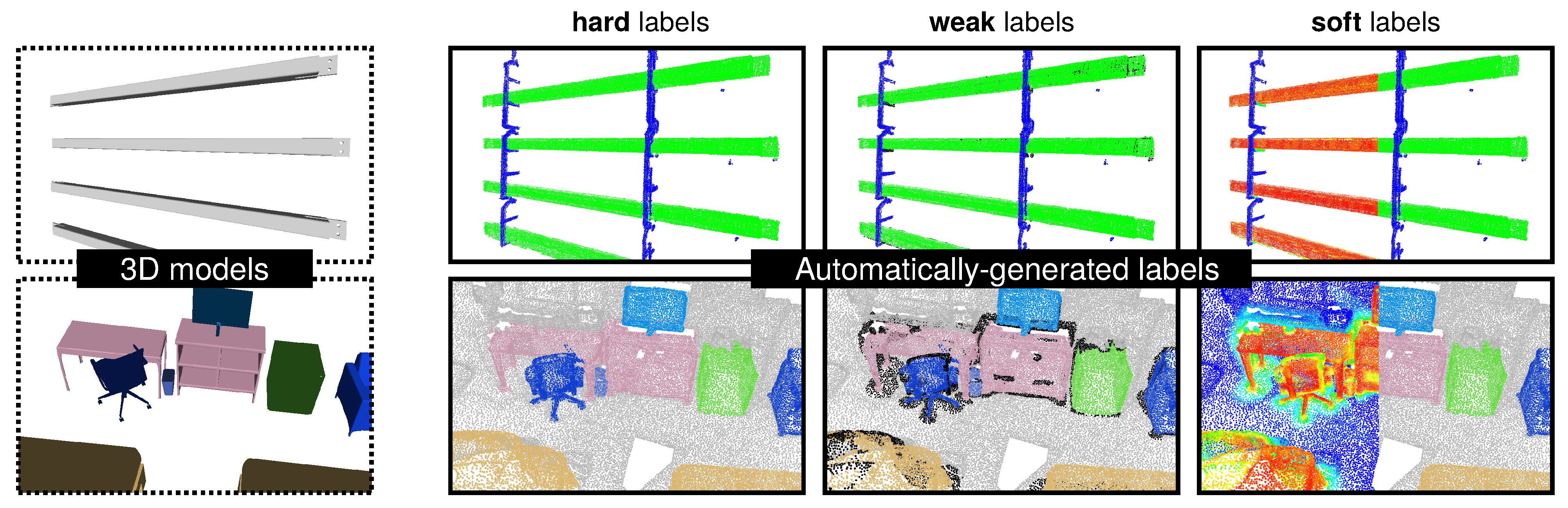
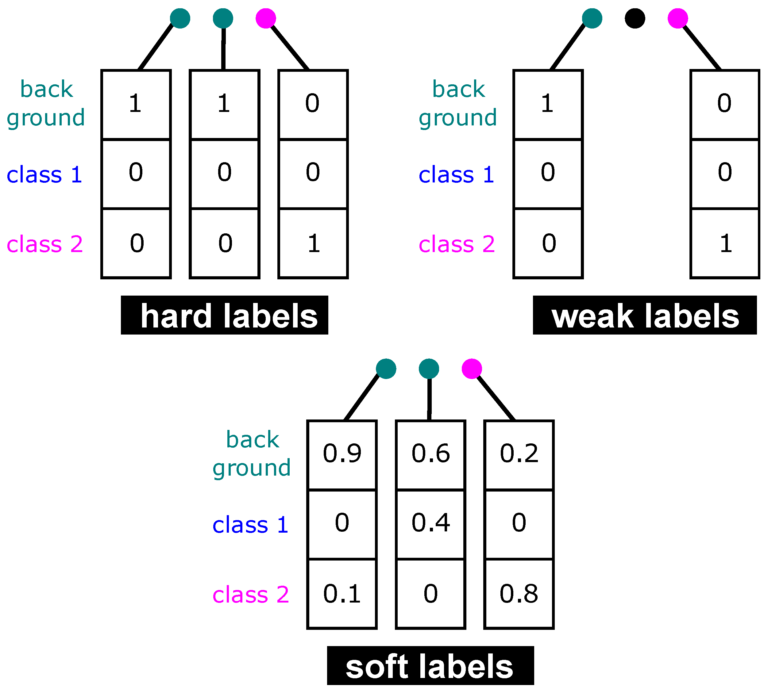
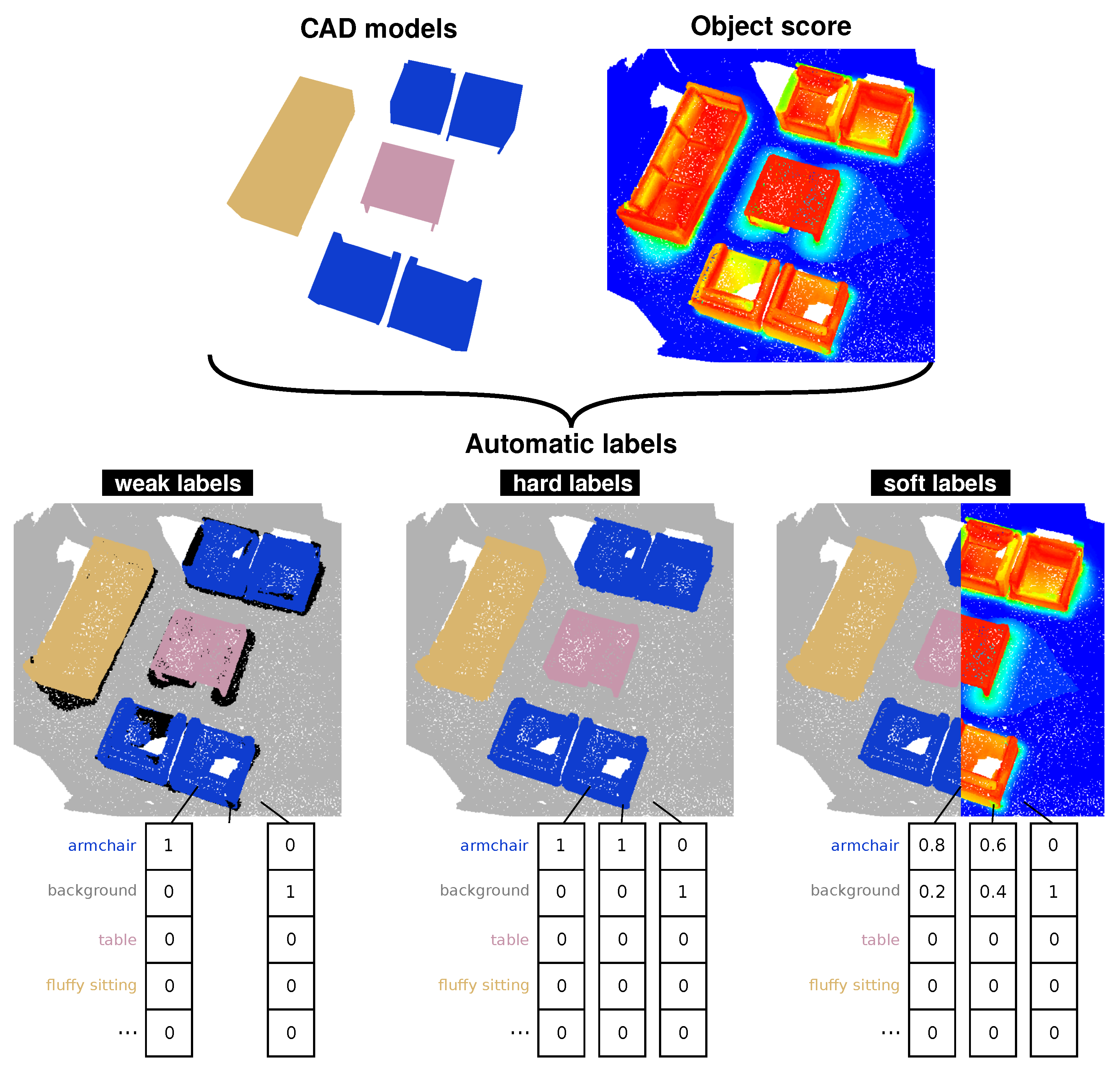
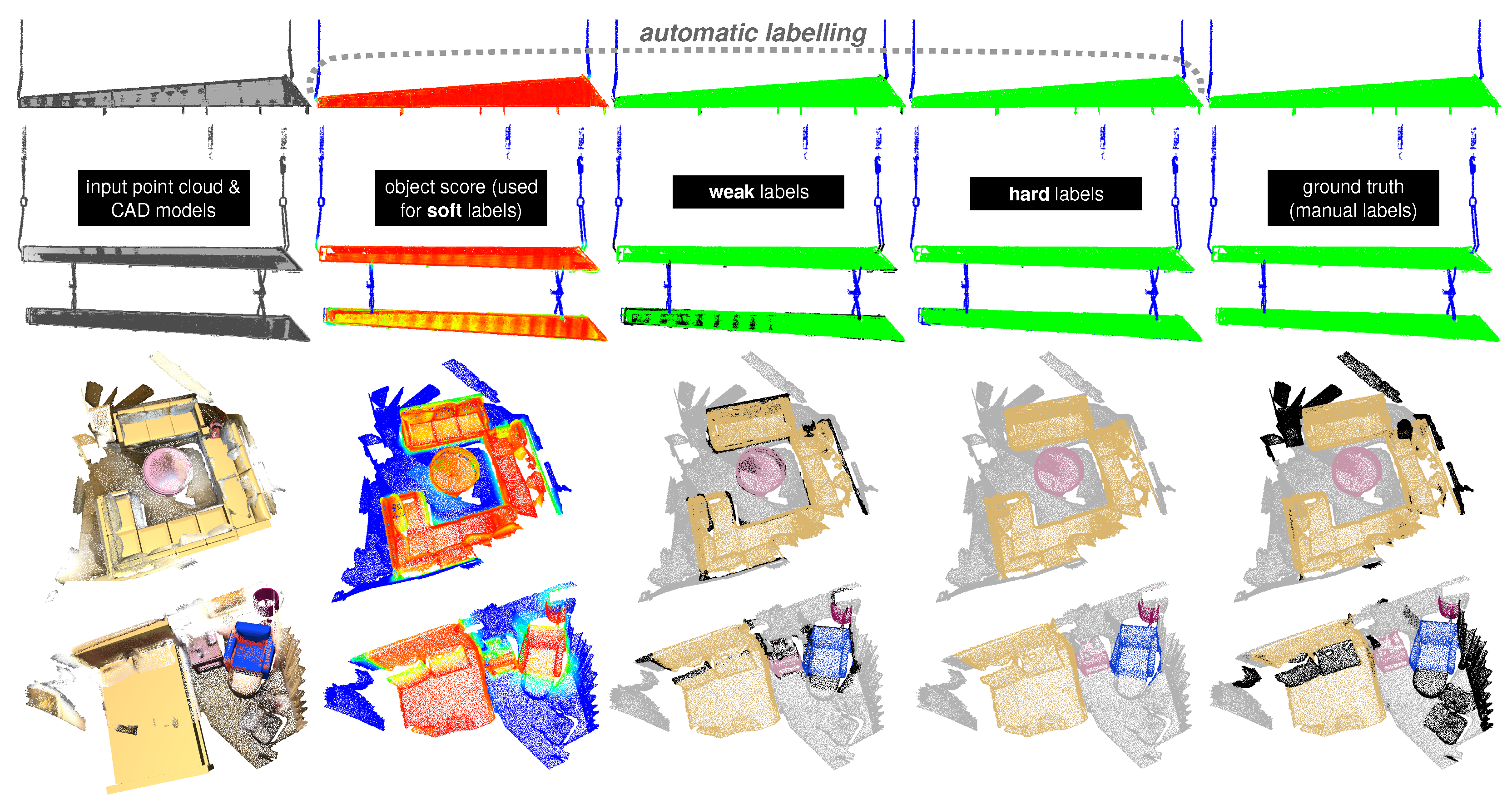
- auto-hard labels: every point is assigned a one-hot label (probability of 1 for the target class, 0 for the other classes)—this is the typical way that labels are defined for semantic segmentation. This annotation scheme does not take into account any uncertainty in the labeling process; during training, the model is equally penalized for wrong predictions in ambiguous regions (where labels are likely to be incorrect) as in easy-to-label regions.
- auto-weak labels: similar to the hard scheme, but points that are ambiguous are left unlabeled (visualized in black throughout the paper). During training, these points are not considered in the loss computation; the model is “free” to predict anything for these unlabeled points without being penalized for it.
- auto-soft labels: the target class and background probability are based on the object score. During training, the model is penalized more for misclassifying easy-to-label points than for misclassifying ambiguous points.
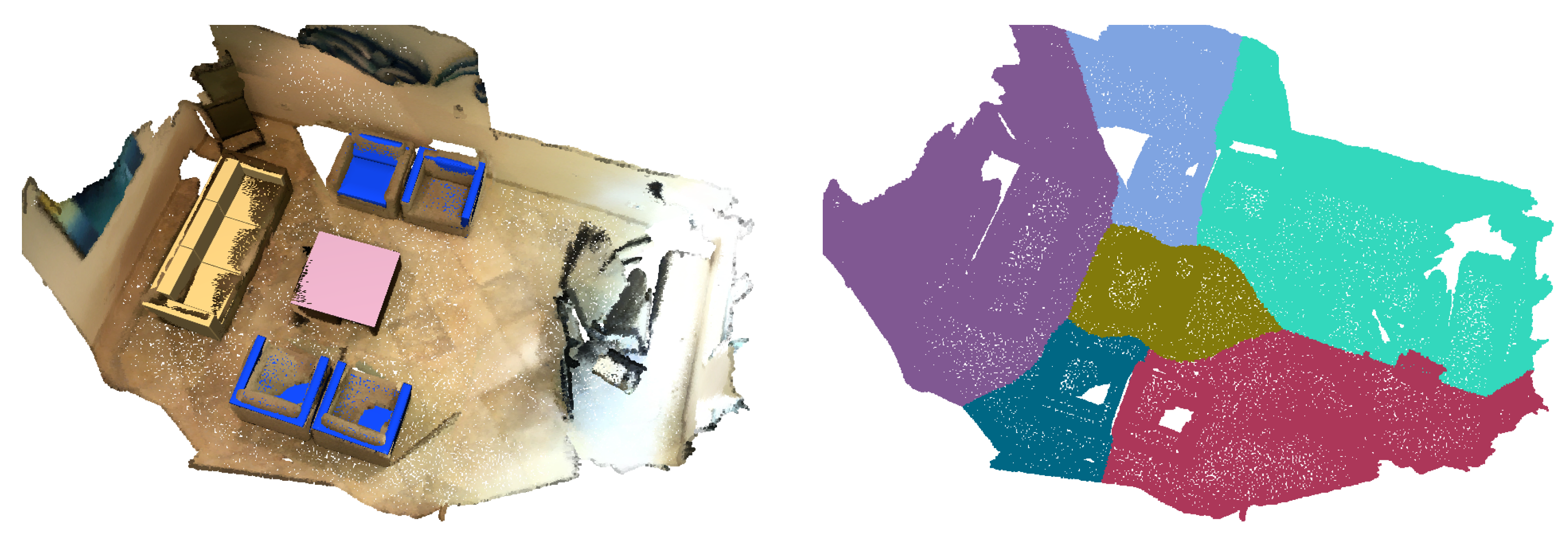
3.1. Divide and Conquer
| Algorithm 1 Point cloud splitting algorithm |
Input: Set of scan points , sequence of M 3D models |
Output:
A section assignment label for each point |
for each point do |
for to M do |
shortest L2 distance between Q and ▹ computed via raycasting |
end for |
end for |
3.2. Zooming in on a Section
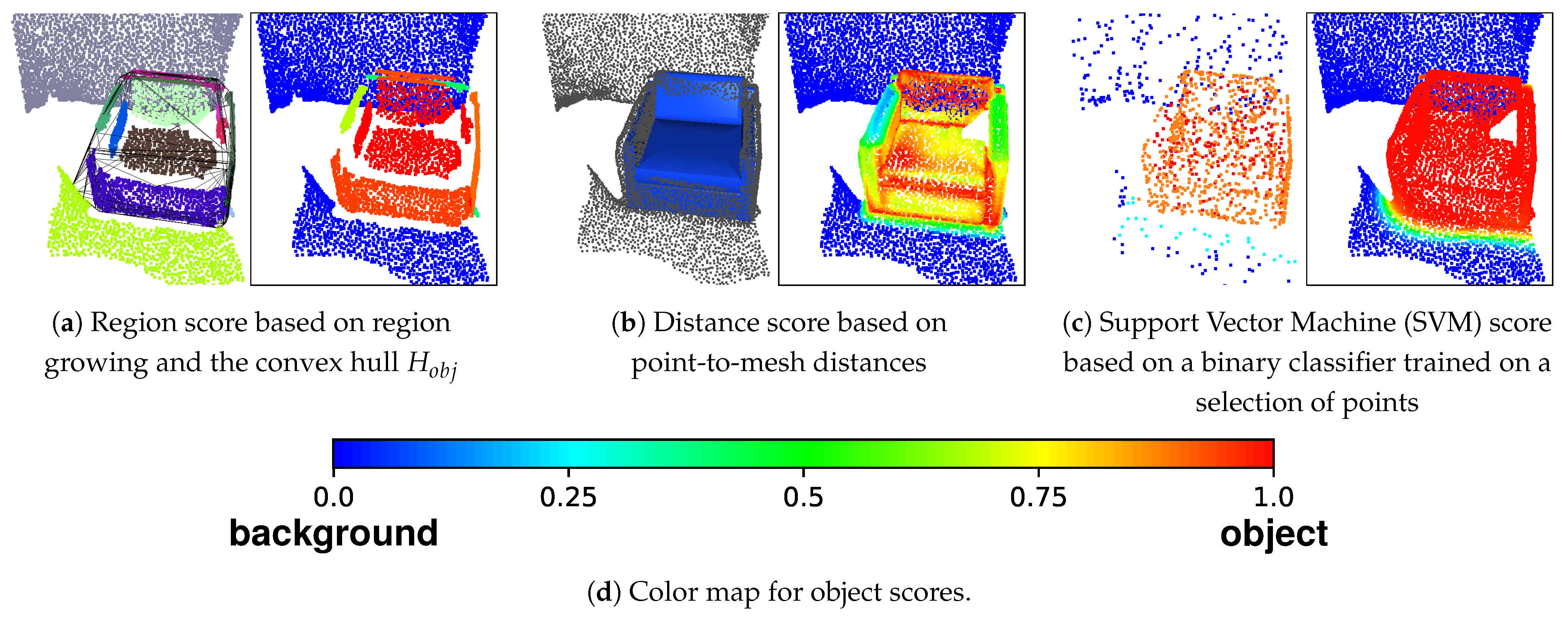
3.2.1. Region Score ()
3.2.2. Distance Score ()
3.2.3. SVM Score
3.3. From Scores to Labels
4. Data
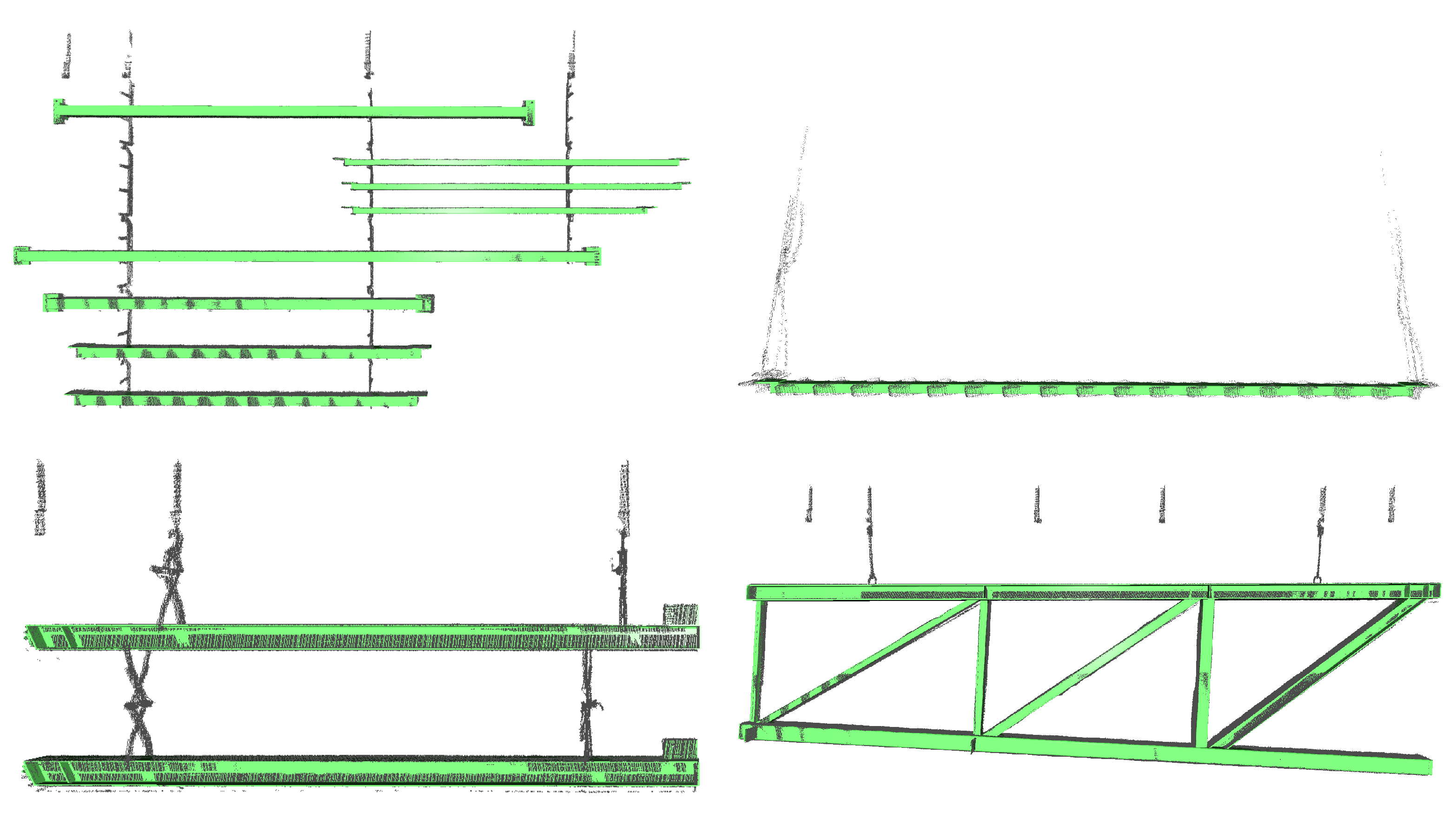
4.1. Beams&Hooks
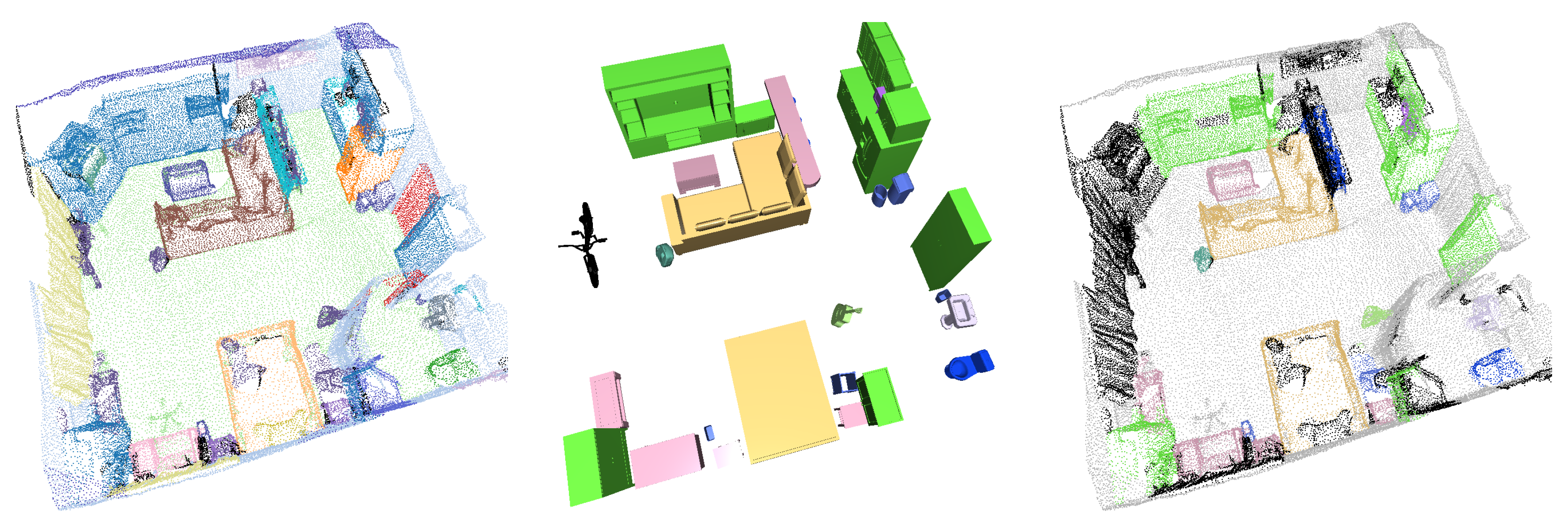
4.2. Scan2CAD
5. Experiments
5.1. Evaluation Procedure
- overall accuracy (OA)—the proportion of correctly classified points (note that this metric can obfuscate poor performance in minority classes)
- mean accuracy (mACC)—class-wise accuracy, averaged across all classes
- mean intersection over union (mIoU)—class-wise IoU, averaged across all classes
- macro-F1—class-wise F1 score, averaged across all classes
5.2. Experiment 1: Automatic vs. Manual Labels
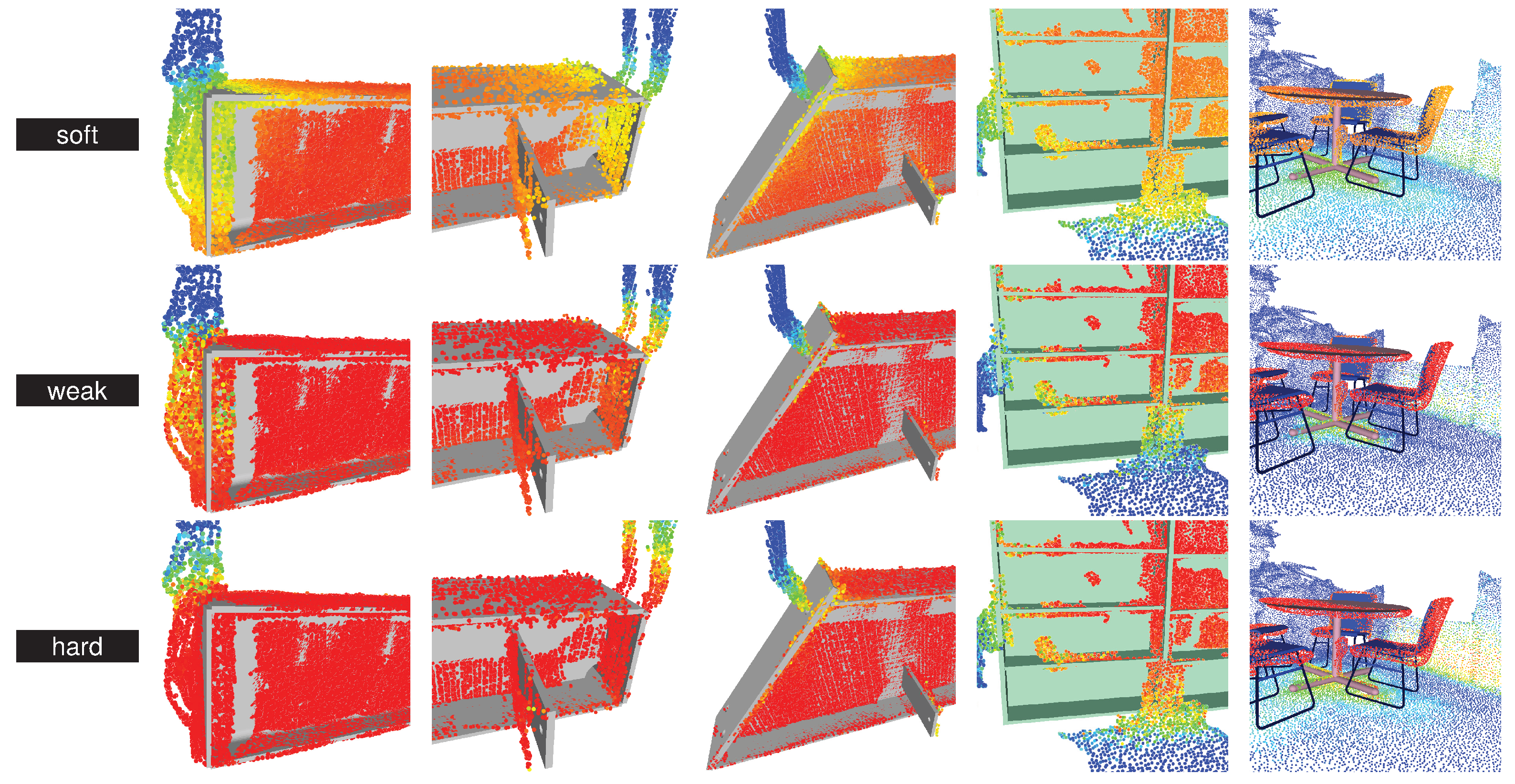
5.2.1. Qualitative Results
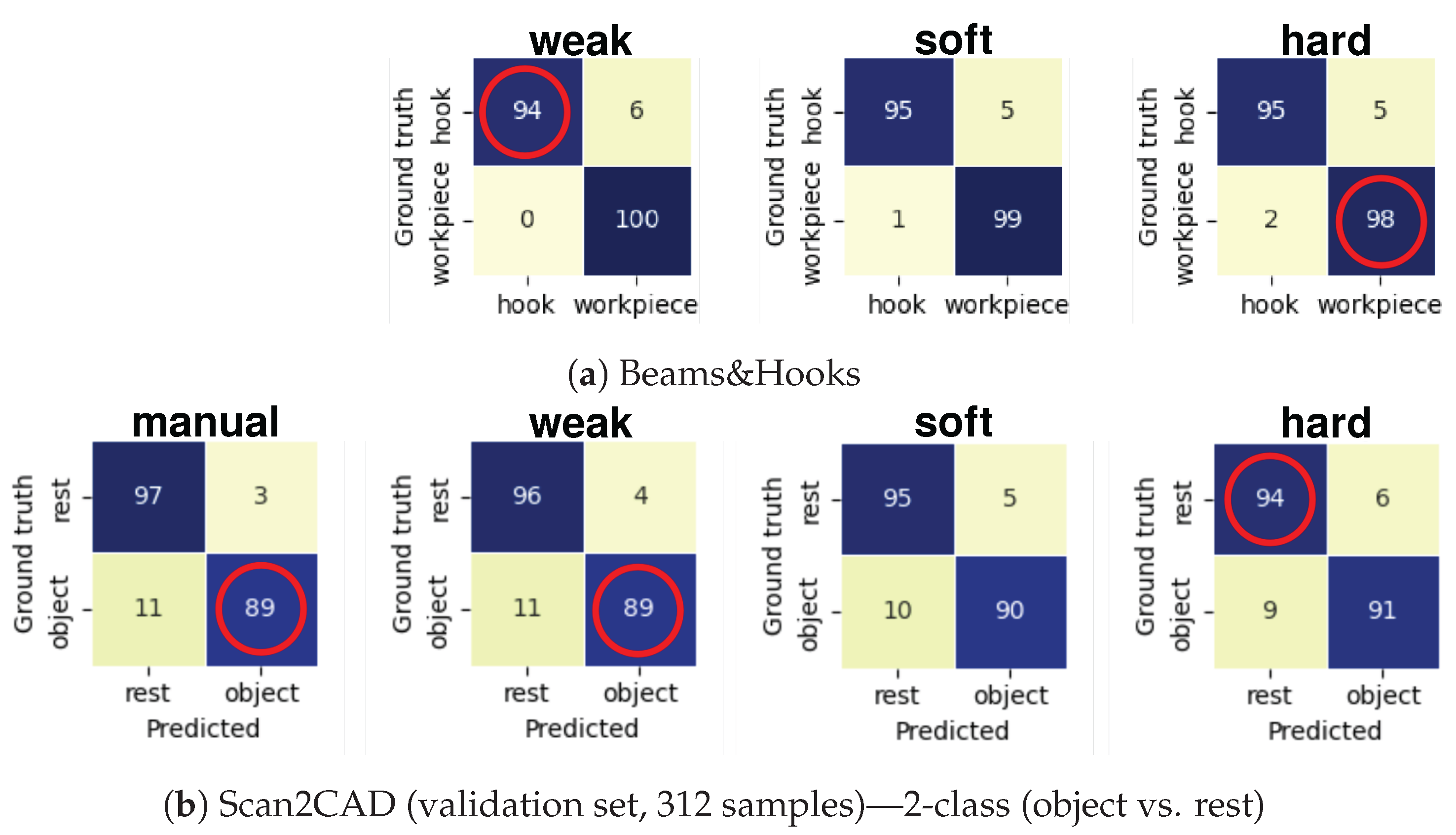
5.2.2. Quantitative Results
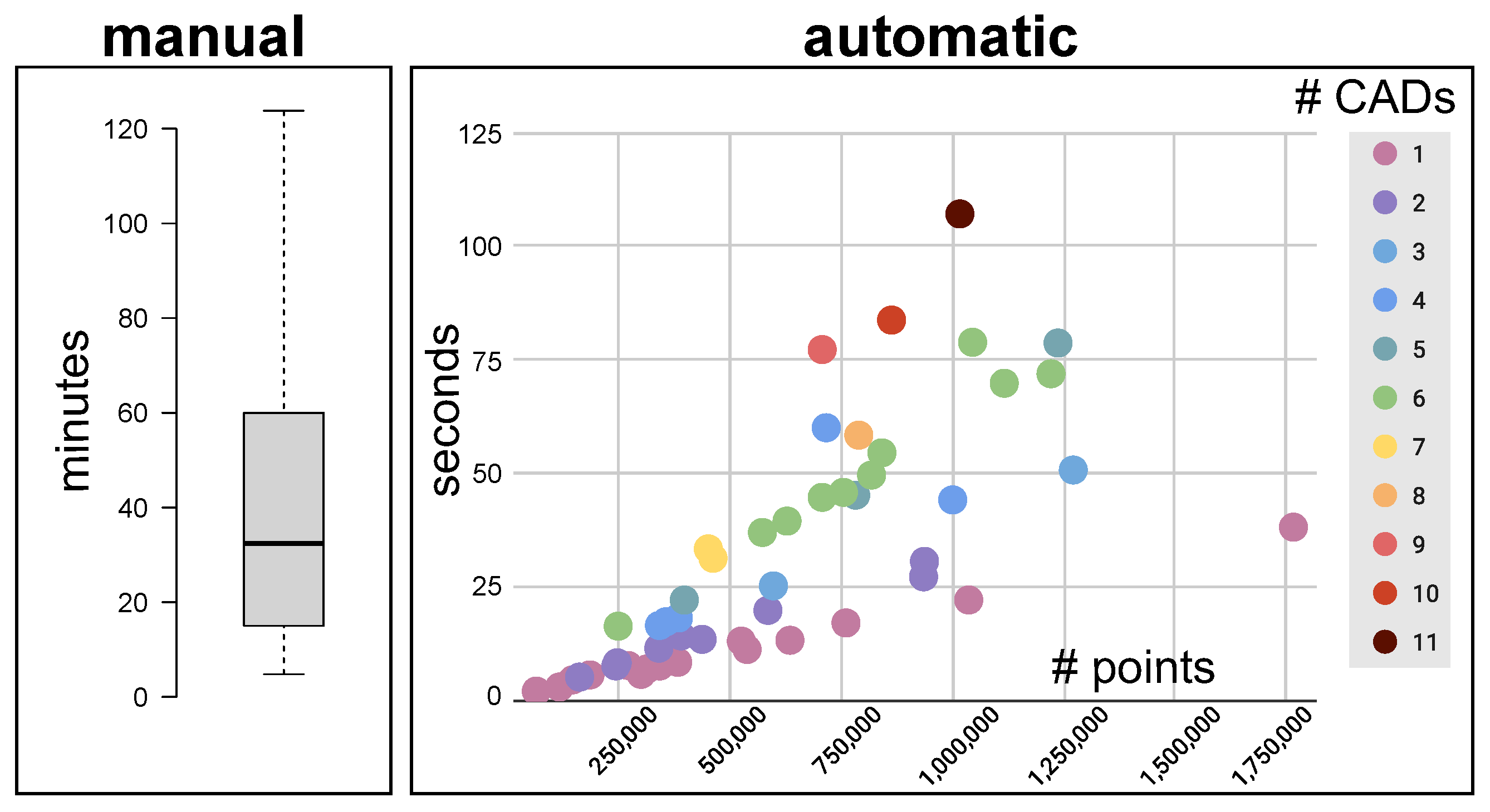
5.2.3. Annotation Time
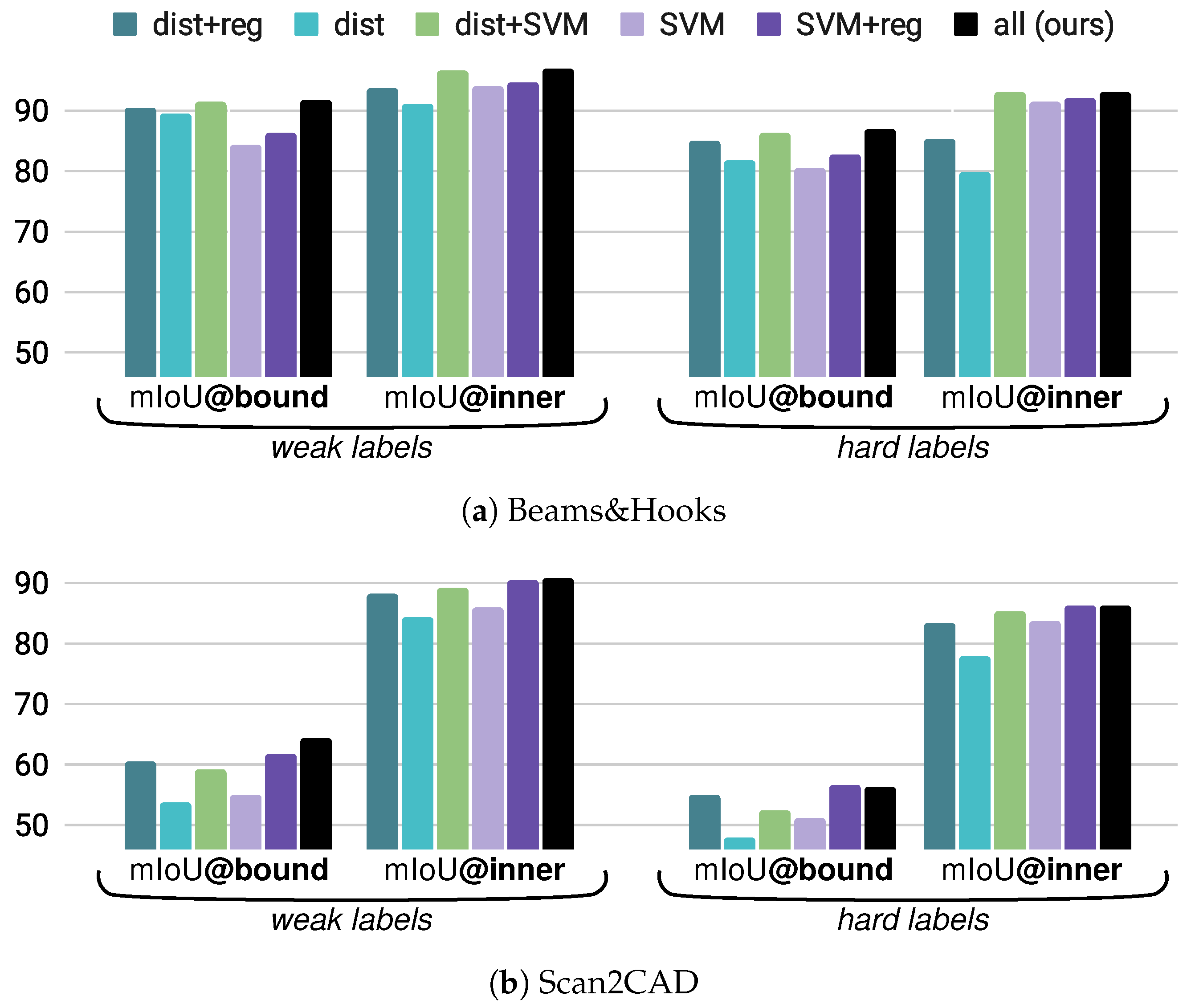
5.2.4. Ablation Study of Labeling Scores
5.3. Experiment 2: Training a Segmentation Model
5.3.1. Architecture and Hyper-Parameters
5.3.2. Dataset Splits
5.3.3. Data Pre-Processing
5.3.4. Results
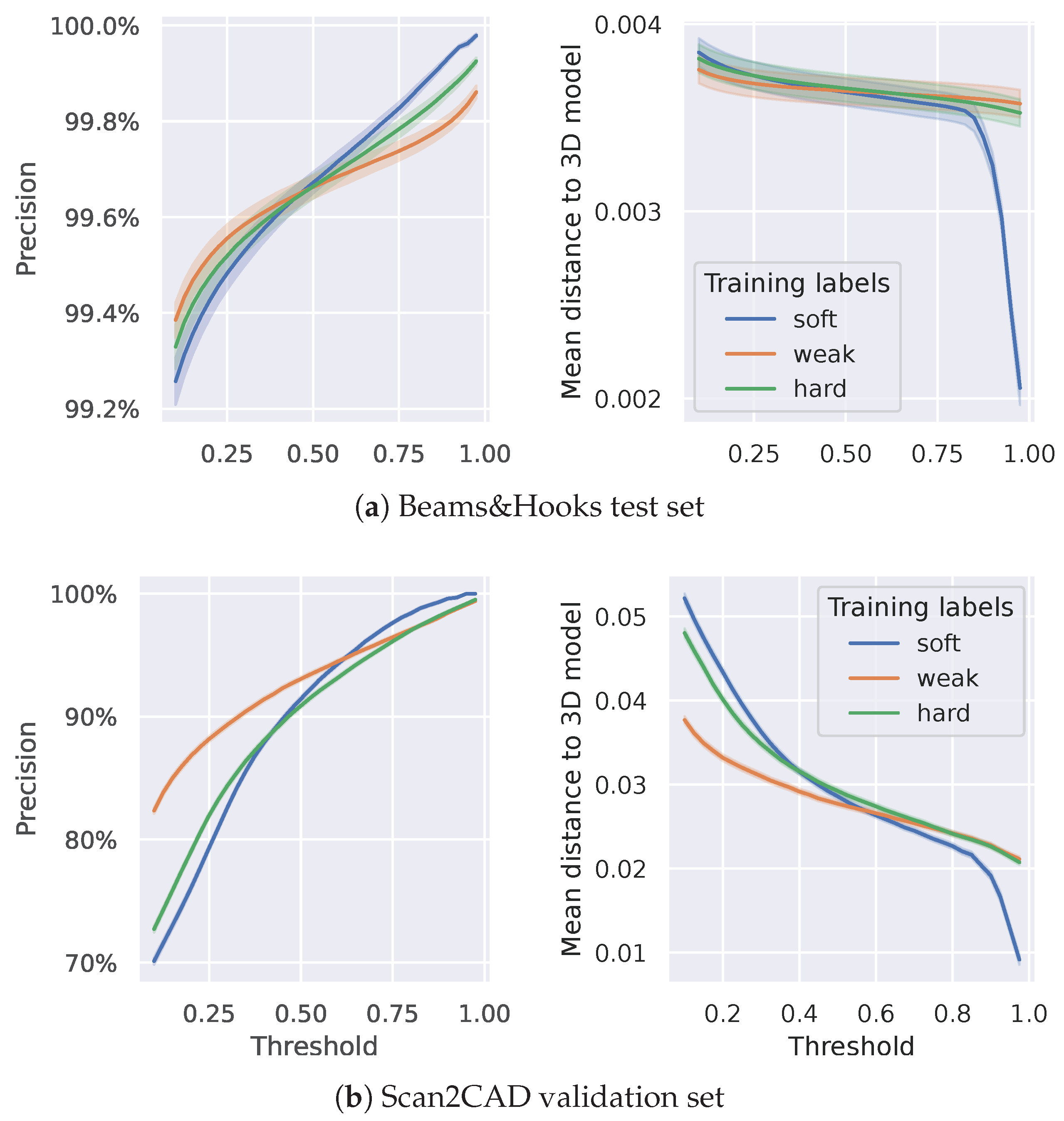
5.3.5. A Closer Look at Soft Predictions
6. Discussion
7. Conclusions
Author Contributions
Funding
Data Availability Statement
Conflicts of Interest
Abbreviations
| BIM | Building Information Modeling |
| CAD | Computer Aided Design |
| DoF | Degree of Freedom |
| IoU | Intersection over Union |
| LiDAR | Light Detection And Ranging |
| OA | Overall Accuracy |
| SVM | Support Vector Machine |
References
- Li, Y.; Ma, L.; Zhong, Z.; Liu, F.; Chapman, M.A.; Cao, D.; Li, J. Deep Learning for LiDAR Point Clouds in Autonomous Driving: A Review. IEEE Trans. Neural Netw. Learn. Syst. 2021, 32, 3412–3432. [Google Scholar] [CrossRef] [PubMed]
- Han, L.; Zheng, T.; Zhu, Y.; Xu, L.; Fang, L. Live Semantic 3D Perception for Immersive Augmented Reality. IEEE Trans. Vis. Comput. Graph. 2020, 26, 2012–2022. [Google Scholar] [CrossRef] [PubMed]
- Xie, Y.; Tian, J.; Zhu, X.X. Linking Points With Labels in 3D: A Review of Point Cloud Semantic Segmentation. IEEE Geosci. Remote Sens. Mag. 2020, 8, 38–59. [Google Scholar] [CrossRef] [Green Version]
- Yang, X.; Xia, D.; Kin, T.; Igarashi, T. IntrA: 3D Intracranial Aneurysm Dataset for Deep Learning. In Proceedings of the IEEE/CVF Conference on Computer Vision and Pattern Recognition (CVPR), Seattle, WA, USA, 13–19 June 2020. [Google Scholar]
- Wang, Q.; Kim, M.K. Applications of 3D point cloud data in the construction industry: A fifteen-year review from 2004 to 2018. Adv. Eng. Inform. 2019, 39, 306–319. [Google Scholar] [CrossRef]
- Guo, Y.; Wang, H.; Hu, Q.; Liu, H.; Liu, L.; Bennamoun, M. Deep Learning for 3D Point Clouds: A Survey. IEEE Trans. Pattern Anal. Mach. Intell. 2021, 43, 4338–4364. [Google Scholar] [CrossRef]
- Toropov, E.; Moura, J. CADillac; Carnegie Mellon University: Pittsburgh, PA, USA, 2019. [Google Scholar] [CrossRef]
- Chen, L.; Sun, J.; Xie, Y.; Zhang, S.; Shuai, Q.; Jiang, Q.; Zhang, G.; Bao, H.; Zhou, X. Shape Prior Guided Instance Disparity Estimation for 3D Object Detection. IEEE Trans. Pattern Anal. Mach. Intell. 2022, 44, 5529–5540. [Google Scholar] [CrossRef]
- Chen, L.C.; Fidler, S.; Yuille, A.L.; Urtasun, R. Beat the MTurkers: Automatic Image Labeling from Weak 3D Supervision. In Proceedings of the IEEE Conference on Computer Vision and Pattern Recognition (CVPR), Columbus, OH, USA, 23–28 June 2014. [Google Scholar]
- Chang, A.X.; Funkhouser, T.; Guibas, L.; Hanrahan, P.; Huang, Q.; Li, Z.; Savarese, S.; Savva, M.; Song, S.; Su, H.; et al. ShapeNet: An Information-Rich 3D Model Repository. Technical Report. arXiv 2015, arXiv:1512.03012. [Google Scholar]
- Xiang, Y.; Kim, W.; Chen, W.; Ji, J.; Choy, C.; Su, H.; Mottaghi, R.; Guibas, L.; Savarese, S. ObjectNet3D: A Large Scale Database for 3D Object Recognition. In Proceedings of the ECCV 2016: Computer Vision—ECCV 2016, Amsterdam, The Netherlands, 11–14 October 2016. [Google Scholar]
- Sun, X.; Wu, J.; Zhang, X.; Zhang, Z.; Zhang, C.; Xue, T.; Tenenbaum, J.B.; Freeman, W.T. Pix3D: Dataset and Methods for Single-Image 3D Shape Modeling. In Proceedings of the IEEE Conference on Computer Vision and Pattern Recognition (CVPR), Salt Lake City, UT, USA, 18–23 June 2018. [Google Scholar]
- Avetisyan, A.; Dahnert, M.; Dai, A.; Savva, M.; Chang, A.X.; Nießner, M. Scan2CAD: Learning CAD Model Alignment in RGB-D Scans. In Proceedings of the 2019 IEEE/CVF Conference on Computer Vision and Pattern Recognition (CVPR), Long Beach, CA, USA, 15–20 June 2019; pp. 2609–2618. [Google Scholar] [CrossRef] [Green Version]
- Dai, A.; Chang, A.X.; Savva, M.; Halber, M.; Funkhouser, T.; Nießner, M. ScanNet: Richly-Annotated 3D Reconstructions of Indoor Scenes. In Proceedings of the 2017 IEEE Conference on Computer Vision and Pattern Recognition (CVPR), Honolulu, HI, USA, 21–26 July 2017; pp. 2432–2443. [Google Scholar] [CrossRef] [Green Version]
- Song, D.; Li, T.B.; Li, W.H.; Nie, W.Z.; Liu, W.; Liu, A.A. Universal Cross-Domain 3D Model Retrieval. IEEE Trans. Multimed. 2021, 23, 2721–2731. [Google Scholar] [CrossRef]
- Arvanitis, G.; Zacharaki, E.I.; Váŝa, L.; Moustakas, K. Broad-to-Narrow Registration and Identification of 3D Objects in Partially Scanned and Cluttered Point Clouds. IEEE Trans. Multimed. 2022, 24, 2230–2245. [Google Scholar] [CrossRef]
- Khalid, M.U.; Hager, J.M.; Kraus, W.; Huber, M.F.; Toussaint, M. Deep Workpiece Region Segmentation for Bin Picking. In Proceedings of the IEEE 15th International Conference on Automation Science and Engineering (CASE), Vancouver, BC, Canada, 22–26 August 2019; pp. 1138–1144. [Google Scholar] [CrossRef] [Green Version]
- Bloembergen, D.; Eijgenstein, C. Automatic labeling of urban point clouds using data fusion. In Proceedings of the 10th International Workshop on Urban Computing at ACM SIGSPATIAL 2021, Beijing, China, 11 November 2021. [Google Scholar]
- Aksoy, E.E.; Baci, S.; Cavdar, S. SalsaNet: Fast Road and Vehicle Segmentation in LiDAR Point Clouds for Autonomous Driving. In Proceedings of the IEEE Intelligent Vehicles Symposium (IV), Las Vegas, NV, USA, 19 October–13 November 2020; pp. 926–932. [Google Scholar] [CrossRef]
- Wang, B.; Wu, V.; Wu, B.; Keutzer, K. LATTE: Accelerating LiDAR Point Cloud Annotation via Sensor Fusion, One-Click Annotation, and Tracking. In Proceedings of the 2019 IEEE Intelligent Transportation Systems Conference (ITSC), Auckland, New Zealand, 27–30 October 2019; pp. 265–272. [Google Scholar] [CrossRef] [Green Version]
- Nguyen, A.; Le, B. 3D point cloud segmentation: A survey. In Proceedings of the 2013 6th IEEE Conference on Robotics, Automation and Mechatronics (RAM), Manila, Philippines, 12–15 November 2013; pp. 225–230. [Google Scholar] [CrossRef]
- Xia, S.; Chen, D.; Wang, R.; Li, J.; Zhang, X. Geometric Primitives in LiDAR Point Clouds: A Review. IEEE J. Sel. Top. Appl. Earth Obs. Remote Sens. 2020, 13, 685–707. [Google Scholar] [CrossRef]
- Su, F.; Zhu, H.; Li, L.; Zhou, G.; Rong, W.; Zuo, X.; Li, W.; Wu, X.; Wang, W.; Yang, F.; et al. Indoor interior segmentation with curved surfaces via global energy optimization. Autom. Constr. 2021, 131, 103886. [Google Scholar] [CrossRef]
- Zhao, B.; Hua, X.; Yu, K.; Xuan, W.; Chen, X.; Tao, W. Indoor Point Cloud Segmentation Using Iterative Gaussian Mapping and Improved Model Fitting. IEEE Trans. Geosci. Remote Sens. 2020, 58, 7890–7907. [Google Scholar] [CrossRef]
- Xu, Y.; Tuttas, S.; Hoegner, L.; Stilla, U. Geometric Primitive Extraction From Point Clouds of Construction Sites Using VGS. IEEE Geosci. Remote Sens. Lett. 2017, 14, 424–428. [Google Scholar] [CrossRef]
- O’Mahony, N.; Campbell, S.; Carvalho, A.; Krpalkova, L.; Riordan, D.; Walsh, J. Point Cloud Annotation Methods for 3D Deep Learning. In Proceedings of the 13th International Conference on Sensing Technology (ICST), Sydney, NSW, Australia, 2–4 December 2019; pp. 1–6. [Google Scholar] [CrossRef]
- Xu, K.; Yao, Y.; Murasaki, K.; Ando, S.; Sagata, A. Semantic Segmentation of Sparsely Annotated 3D Point Clouds by Pseudo-labeling. In Proceedings of the International Conference on 3D Vision (3DV), Quebec City, QC, Canada, 16–19 September 2019; pp. 463–471. [Google Scholar] [CrossRef]
- Luo, H.; Zheng, Q.; Wang, C.; Guo, W. Boundary-Aware and Semiautomatic Segmentation of 3-D Object in Point Clouds. IEEE Geosci. Remote Sens. Lett. 2021, 18, 910–914. [Google Scholar] [CrossRef]
- Xu, X.; Lee, G.H. Weakly Supervised Semantic Point Cloud Segmentation: Towards 10× Fewer Labels. In Proceedings of the 2020 IEEE/CVF Conference on Computer Vision and Pattern Recognition (CVPR), Seattle, WA, USA, 13–19 June 2020; pp. 13703–13712. [Google Scholar] [CrossRef]
- Unal, O.; Dai, D.; Van Gool, L. Scribble-supervised lidar semantic segmentation. In Proceedings of the IEEE/CVF Conference on Computer Vision and Pattern Recognition (CVPR), New Orleans, LA, USA, 18–24 June 2022; pp. 2697–2707. [Google Scholar]
- Nivaggioli, A.; Hullo, J.F.; Thibault, G. Using 3D models to generate labels for panoptic segmentation of industrial scenes. ISPRS Ann. Photogramm. Remote Sens. Spat. Inf. Sci. 2019, IV-2/W5, 61–68. [Google Scholar] [CrossRef] [Green Version]
- Faltermeier, F.L.; Krapf, S.; Willenborg, B.; Kolbe, T.H. Improving Semantic Segmentation of Roof Segments Using Large-Scale Datasets Derived from 3D City Models and High-Resolution Aerial Imagery. Remote Sens. 2023, 15, 1931. [Google Scholar] [CrossRef]
- Yao, Z.; Nagel, C.; Kunde, F.; Hudra, G.; Willkomm, P.; Donaubauer, A.; Adolphi, T.; Kolbe, T.H. 3DCityDB - a 3D geodatabase solution for the management, analysis, and visualization of semantic 3D city models based on CityGML. Open Geospat. Data Softw. Stand. 2018, 3, 5. [Google Scholar] [CrossRef] [Green Version]
- Lai, K.; Bo, L.; Fox, D. Unsupervised feature learning for 3D scene labeling. In Proceedings of the 2014 IEEE International Conference on Robotics and Automation (ICRA), Hong Kong, China, 31 May–7 June 2014; pp. 3050–3057. [Google Scholar] [CrossRef]
- Colligan, A.R.; Robinson, T.T.; Nolan, D.C.; Hua, Y. Point Cloud Dataset Creation for Machine Learning on CAD Models. Comput.-Aided Des. Appl. 2021, 18, 760–771. [Google Scholar] [CrossRef]
- Wang, F.; Zhuang, Y.; Gu, H.; Hu, H. Automatic Generation of Synthetic LiDAR Point Clouds for 3-D Data. IEEE Trans. Instrum. Meas. Anal. 2019, 68, 2671–2673. [Google Scholar] [CrossRef] [Green Version]
- Ma, J.W.; Czerniawski, T.; Leite, F. Semantic segmentation of point clouds of building interiors with deep learning: Augmenting training datasets with synthetic BIM-based point clouds. Autom. Constr. 2020, 113, 103144. [Google Scholar] [CrossRef]
- De Geyter, S.; Bassier, M.; Vergauwen, M. Automated Training Data Creation for Semantic Segmentation of 3D Point Clouds. Int. Arch. Photogramm. Remote Sens. Spat. Inf. Sci. 2022, XLVI-5/W1-2022, 59–67. [Google Scholar] [CrossRef]
- Gao, B.; Xing, C.; Xie, C.; Wu, J.; Geng, X. Deep Label Distribution Learning With Label Ambiguity. IEEE Trans. Image Process. 2017, 26, 2825–2838. [Google Scholar] [CrossRef] [PubMed] [Green Version]
- Szegedy, C.; Vanhoucke, V.; Ioffe, S.; Shlens, J.; Wojna, Z. Rethinking the Inception Architecture for Computer Vision. In Proceedings of the 2016 IEEE Conference on Computer Vision and Pattern Recognition (CVPR), Las Vegas, NV, USA, 27–30 June 2016; pp. 2818–2826. [Google Scholar] [CrossRef] [Green Version]
- Zhang, C.; Jiang, P.; Hou, Q.; Wei, Y.; Han, Q.; Li, Z.; Cheng, M. Delving Deep into Label Smoothing. IEEE Trans. Image Process. 2021, 30, 5984–5996. [Google Scholar] [CrossRef] [PubMed]
- Díaz, R.; Marathe, A. Soft Labels for Ordinal Regression. In Proceedings of the 2019 IEEE/CVF Conference on Computer Vision and Pattern Recognition (CVPR), Long Beach, CA, USA, 15–20 June 2019; pp. 4733–4742. [Google Scholar] [CrossRef]
- Bertinetto, L.; Mueller, R.; Tertikas, K.; Samangooei, S.; Lord, N.A. Making Better Mistakes: Leveraging Class Hierarchies With Deep Networks. In Proceedings of the 2020 IEEE/CVF Conference on Computer Vision and Pattern Recognition (CVPR), Seattle, WA, USA, 13–19 June 2020; pp. 12503–12512. [Google Scholar] [CrossRef]
- Humblot-Renaux, G.; Marchegiani, L.; Moeslund, T.B.; Gade, R. Navigation-Oriented Scene Understanding for Robotic Autonomy: Learning to Segment Driveability in Egocentric Images. IEEE Robot. Autom. Lett. 2022, 7, 2913–2920. [Google Scholar] [CrossRef]
- Gros, C.; Lemay, A.; Cohen-Adad, J. SoftSeg: Advantages of soft versus binary training for image segmentation. Med. Image Anal. 2021, 71, 102038. [Google Scholar] [CrossRef]
- Lüddecke, T.; Wörgötter, F. Fine-grained action plausibility rating. Robot. Auton. Syst. 2020, 129, 103511. [Google Scholar] [CrossRef]
- Qian, G.; Li, Y.; Peng, H.; Mai, J.; Hammoud, H.; Elhoseiny, M.; Ghanem, B. PointNeXt: Revisiting PointNet++ with Improved Training and Scaling Strategies. Adv. Neural Inf. Process. Syst. 2022, 35, 23192–23204. [Google Scholar]
- Rabbani, T.; van den Heuvel, F.; Vosselman, G. Segmentation of point clouds using smoothness constraints. In Proceedings of the ISPRS Commission V Symposium ’Image Engineering and Vision Metrology’, Dresden, Germany, 25–27 September 2006; Volume 35, pp. 248–253. [Google Scholar]
- Cortes, C.; Vapnik, V. Support-Vector Networks. Mach. Learn. 1995, 20, 273–297. [Google Scholar] [CrossRef]
- Chang, C.C.; Lin, C.J. LIBSVM: A Library for Support Vector Machines. ACM Trans. Intell. Syst. Technol. 2011, 2, 27. [Google Scholar] [CrossRef]
- Bi, Z.M.; Lang, S.Y.T. A Framework for CAD- and Sensor-Based Robotic Coating Automation. IEEE Trans. Ind. Inform. 2007, 3, 84–91. [Google Scholar] [CrossRef]
- Ge, J.; Li, J.; Peng, Y.; Lu, H.; Li, S.; Zhang, H.; Xiao, C.; Wang, Y. Online 3-D Modeling of Complex Workpieces for the Robotic Spray Painting With Low-Cost RGB-D Cameras. IEEE Trans. Instrum. Meas. 2021, 70, 5011013. [Google Scholar] [CrossRef]
- Tang, L.; Zhan, Y.; Chen, Z.; Yu, B.; Tao, D. Contrastive Boundary Learning for Point Cloud Segmentation. In Proceedings of the IEEE/CVF Conference on Computer Vision and Pattern Recognition (CVPR), New Orleans, LA, USA, 18–24 June 2022; pp. 8489–8499. [Google Scholar]
- Qi, C.R.; Yi, L.; Su, H.; Guibas, L.J. PointNet++: Deep Hierarchical Feature Learning on Point Sets in a Metric Space. In Proceedings of the NIPS’17, Long Beach, CA, USA, 4–9 December 2017; pp. 5105–5114. [Google Scholar]
- Charles, R.Q.; Su, H.; Kaichun, M.; Guibas, L.J. PointNet: Deep Learning on Point Sets for 3D Classification and Segmentation. In Proceedings of the 2017 IEEE Conference on Computer Vision and Pattern Recognition (CVPR), Honolulu, HI, USA, 24–26 July 2017; pp. 77–85. [Google Scholar] [CrossRef] [Green Version]
- Kingma, D.P.; Ba, J. Adam: A Method for Stochastic Optimization. arxiv 2014, arXiv:1412.6980. [Google Scholar]
- Sørensen, T.; Mark, N.; Møgelmose, A. A RANSAC Based CAD Mesh Reconstruction Method Using Point Clustering for Mesh Connectivity. In Proceedings of the International Conference on Machine Vision and Applications, Aichi, Japan, 25–27 July 2021; 4th ed; pp. 61–65. [Google Scholar] [CrossRef]
- Wei, J.; Hu, L.; Wang, C.; Kneip, L. Accurate Instance-Level CAD Model Retrieval in a Large-Scale Database. In Proceedings of the 2022 IEEE/RSJ International Conference on Intelligent Robots and Systems (IROS), Kyoto, Japan, 23–27 October 2022; pp. 9879–9885. [Google Scholar] [CrossRef]
- Zhao, T.; Feng, Q.; Jadhav, S.; Atanasov, N. CORSAIR: Convolutional Object Retrieval and Symmetry-AIded Registration. In Proceedings of the 2021 IEEE/RSJ International Conference on Intelligent Robots and Systems (IROS), Prague, Czech Republic, 27 September–1 October 2021; pp. 47–54. [Google Scholar] [CrossRef]
- Uy, M.A.; Kim, V.G.; Sung, M.; Aigerman, N.; Chaudhuri, S.; Guibas, L.J. Joint Learning of 3D Shape Retrieval and Deformation. In Proceedings of the IEEE/CVF Conference on Computer Vision and Pattern Recognition (CVPR), Nashville, TN, USA, 20–25 June 2021; pp. 11713–11722. [Google Scholar]
- Piewak, F.; Pinggera, P.; Schäfer, M.; Peter, D.; Schwarz, B.; Schneider, N.; Enzweiler, M.; Pfeiffer, D.; Zöllner, M. Boosting LiDAR-Based Semantic Labeling by Cross-modal Training Data Generation. In Proceedings of the Computer Vision—ECCV 2018 Workshops, Munich, Germany, 8–14 September 2018; pp. 497–513. [Google Scholar]


| Class | Points | w |
|---|---|---|
| object | 10 | |
| 5 | ||
| background | 1 | |
| 10 |
| Dataset | #Classes | #Scans | Avg. #Points per Scan | Unique CADs | Avg. #CADs per Scan |
|---|---|---|---|---|---|
| Beams&Hooks | 2 | 775 | 798,315 | 149 | 5.2 |
| Scan2CAD | 13 | 1506 | 147,941 | 3049 | 9.4 |
| (a) Beams&Hooks (test set, 50 samples) | |||||||
| labels | % labeled | OA | mACC | macro-F1 | mIoU | ||
| overall | @bound. | @inner | |||||
| auto-hard | 100 | 99.07 | 97.81 | 96.21 | 93.30 | 86.80 | 93.16 |
| auto-weak | 95.02 | 99.52 | 98.97 | 98.37 | 96.95 | 91.88 | 96.81 |
| (b) Scan2CAD (validation set, 312 samples) | |||||||
| labels | % labeled | OA | mACC | macro-F1 | mIoU | ||
| overall | @bound. | @inner | |||||
| auto-hard | 100 | 93.15 | 88.92 | 88.28 | 80.81 | 56.42 | 86.13 |
| auto-weak | 89.42 | 96.00 | 91.75 | 91.91 | 86.95 | 64.43 | 90.81 |
| (a) Beams&Hooks (test set, 50 samples) | ||||||
|---|---|---|---|---|---|---|
| training labels | OA | mACC | macro-F1 | mIoU | ||
| overall | @bound. | @inner | ||||
| auto-hard | 97.37 | 95.51 | 94.78 | 91.36 | 75.74 | 93.66 |
| auto-weak | 99.27 | 96.35 | 96.97 | 94.26 | 76.64 | 97.86 |
| auto-soft | 99.13 | 96.67 | 96.58 | 93.68 | 78.64 | 96.63 |
| (b) Scan2CAD (validation set, 312 samples)—13-class | ||||||
| training labels | OA | mACC | macro-F1 | mIoU | ||
| overall | @bound. | @inner | ||||
| manual | 87.40 | 47.63 | 47.97 | 41.56 | 25.57 | 45.44 |
| auto-hard | 86.06 | 46.85 | 46.59 | 40.44 | 25.99 | 44.12 |
| auto-weak | 86.78 | 48.97 | 49.53 | 42.07 | 26.08 | 45.67 |
| auto-soft | 86.47 | 48.58 | 49.43 | 42.40 | 25.78 | 46.41 |
Disclaimer/Publisher’s Note: The statements, opinions and data contained in all publications are solely those of the individual author(s) and contributor(s) and not of MDPI and/or the editor(s). MDPI and/or the editor(s) disclaim responsibility for any injury to people or property resulting from any ideas, methods, instructions or products referred to in the content. |
© 2023 by the authors. Licensee MDPI, Basel, Switzerland. This article is an open access article distributed under the terms and conditions of the Creative Commons Attribution (CC BY) license (https://creativecommons.org/licenses/by/4.0/).
Share and Cite
Humblot-Renaux, G.; Jensen, S.B.; Møgelmose, A. From CAD Models to Soft Point Cloud Labels: An Automatic Annotation Pipeline for Cheaply Supervised 3D Semantic Segmentation. Remote Sens. 2023, 15, 3578. https://doi.org/10.3390/rs15143578
Humblot-Renaux G, Jensen SB, Møgelmose A. From CAD Models to Soft Point Cloud Labels: An Automatic Annotation Pipeline for Cheaply Supervised 3D Semantic Segmentation. Remote Sensing. 2023; 15(14):3578. https://doi.org/10.3390/rs15143578
Chicago/Turabian StyleHumblot-Renaux, Galadrielle, Simon Buus Jensen, and Andreas Møgelmose. 2023. "From CAD Models to Soft Point Cloud Labels: An Automatic Annotation Pipeline for Cheaply Supervised 3D Semantic Segmentation" Remote Sensing 15, no. 14: 3578. https://doi.org/10.3390/rs15143578