A Novel Technique for High-Precision Ionospheric VTEC Estimation and Prediction at the Equatorial Ionization Anomaly Region: A Case Study over Haikou Station

Abstract

This paper introduces a novel technique that uses observation data from GNSS to estimate the ionospheric vertical total electron content (VTEC) using the Kriging–Kalman method. The technique provides a method to validate the accuracy of the Ionospheric VTEC analysis within the Equatorial Ionization anomaly region. The technique developed uses GNSS VTEC alongside solar parameters, such as solar radio flux (F10.7 cm), Disturbance Storm Time (Dst) and other data, and Long Short Term Memory (LSTM) Networks to predict the occurrence time of the ionospheric equatorial anomaly and ionospheric VTEC changes. The LSTM method was applied to GNSS data from Haikou Station. A comparison of this technique with the neural network (NN) model and International Reference Ionosphere model shows that the LSTM outperforms all of them at VTEC estimation and prediction. The results, which are based on the root mean square error (RMSE) between GNSS VTEC and GIM VTEC outside the equatorial anomaly region, was 1.42 TECU, and the results of GNSS VTEC and VTEC from Beidou geostationary orbit satellite, which lies inside the equatorial ionization anomaly region, was 1.92 TECU. The method developed can be used in VTEC prediction and estimation in real time space operations.

1. Introduction

The ionosphere is closely associated with human life. Natural disasters (e.g., typhoons and earthquakes) and human activities (e.g., nuclear explosions and rocket launches) can affect the ionosphere [1,2]. Many low-orbit spacecrafts operate in the ionosphere. High-tech systems based on short-wave and satellite-ground radio links (such as short-wave communications and satellite positioning) are affected by the ionosphere [3,4]. For the ultra high frequency band, the distance error caused by the ionosphere in the equatorial anomaly region is hundreds of meters or more. Ionospheric error delays have a significant impact on the performance of radar, measurement and control, navigation, communication, and other equipment. Ionospheric TEC is an important parameter for measuring its spatiotemporal variation. Accurate monitoring and forecasting of the TEC are of great significance.

Owing to the large spatial scale of the ionosphere and the many factors affecting its internal changes, various complex physical and chemical processes occur in the ionosphere [5,6]. At the middle and low latitudes, the presence of equatorial ionization anomaly region greatly impacts the local physical electrodynamics, making it so difficult to accurately develop a model for the region [7,8,9]. Several efforts in modeling the ionospheric dynamics have been achieved over the last decades of research, such as The Thermosphere–Ionosphere–Mesosphere Electrodynamics General Circulation Model (TIME-GCM) [10], The Coupled Thermosphere Ionosphere Model (CTIM) [11], and The Global Ionosphere Thermosphere Model (GITM) [12]. These physical models are less limited by data sources; however, the inversion accuracy depends on the accuracy of the given initial conditions and external driving parameters. With the increase in the number of ionospheric observation data, many scholars have established empirical ionospheric models—such as NeQuick, Klobuchar and IRI [13,14,15] based on a large amount of observational data. These empirical models have medium- and long-term prediction capabilities; however, models built based on statistical methods lead to poor estimation and prediction accuracies.

High-precision ionospheric TEC estimation requires an accurate calculation of the system hardware delay (i.e., differential code bias or DCB) of the receiver and satellite. Currently, the main solution methods are the grid condition constraint, polynomial model, spherical harmonic function methods [16,17,18], as well as the Kalman method [19,20]. In low-latitude regions, particularly in the equatorial anomaly region, ionospheric TEC results obtained using the above system hardware delay solution method cannot accurately reflect the real changes in the ionospheric TEC in the region, which adversely affect the accuracy in the performance of ionospheric TEC prediction models [21,22]. Therefore, it is necessary to further study high-precision estimation methods of ionospheric TEC to improve the accuracy of ionospheric TEC calculations in the equatorial anomaly region.

With the gradual increase in ionospheric observation means and data, the use of artificial intelligence methods to model complex processes in the ionosphere and carry out ionospheric TEC prediction has become the current research focus. In the literature [23,24,25,26,27], ionospheric TEC single-point or regional prediction was realized using a neural network model. Because ionospheric TECs are essentially a time-series data, with the continuous development and improvement of deep learning models, an increasing number of scholars have tried to improve the accuracy of ionospheric TEC single point or regional prediction using models such as the convolutional neural network and LSTM [28,29,30,31,32] and have achieved good results. In this work, we focus on using the LSTM method and observations from Haikou Station to develop a novel approach to enable VTEC estimation and prediction within the Equatorial Ionization anomaly region.

The paper is divided into five sections, beginning with a brief description of the importance of ionospheric VTEC research and the current methods for estimating and predicting ionospheric VTEC. Section 2 provides an improved ionospheric VTEC estimation method and explains the ionospheric VTEC prediction method. A new method for evaluating the accuracy of ionospheric VTEC has been proposed and the prediction accuracy of different ionospheric VTEC prediction models has been analyzed in Section 3. Section 4 provides a discussion on the results of ionospheric VTEC estimation and prediction experiments. The conclusions are given in Section 5. The results of this study can be applied to the high-precision refraction error correction of the equatorial anomaly area radar to improve the early warning ability of radar for severe changes in ionospheric TEC in the equatorial anomaly area.

2. Materials and Methods

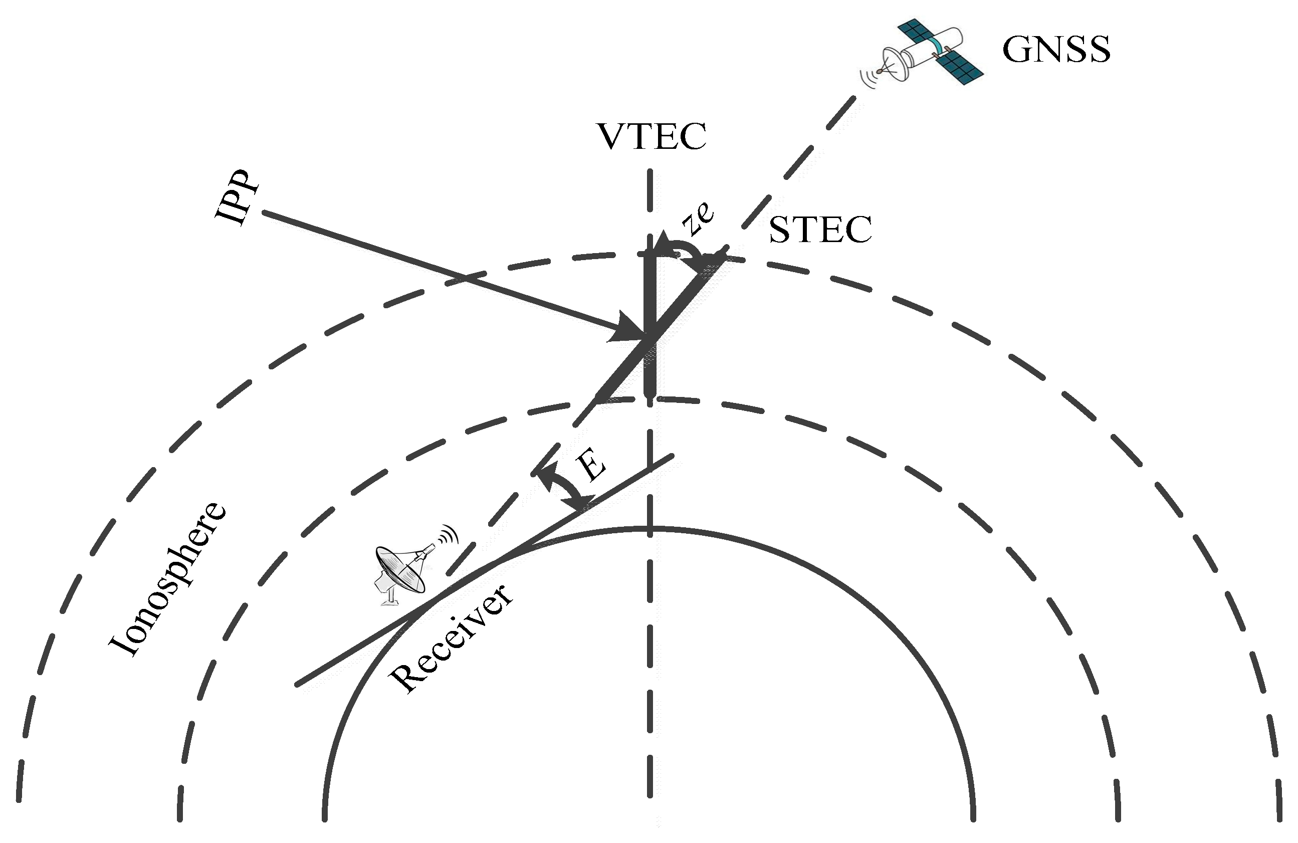
2.1. Ionospheric VTEC Estimation Method

The ionosphere is a dispersive medium and the time delay caused by radio waves of different frequencies passing through it varies. Using the different delays of the ionosphere to the different frequency signals passing through it, the GNSS signal dual-frequency coherence method was used to realize the ionospheric TEC inversion on the signal propagation path. The implementation process is illustrated in Figure 1.

The influence of the ionosphere on GNSS signals can be approximated using the following formulas:

$$n_p\approx 1-\frac{40.28}{f^2}Ne$$

(1)

$$n_g=n_p+f\frac{\partial n_p}{\partial f}\approx 1+\frac{40.28}{f^2}Ne$$

(2)

where $n_p$ and $n_g$ are the phase refractive index and group refractive index of the GNSS signal in the ionosphere, respectively; $f$(Hz) is the GNSS signal frequency; and $N_e$($el/m^2$) is the ionospheric electron density.

When a GNSS signal propagates in the ionosphere, the ionospheric delays $I_P$ and $I_L$ corresponding to the pseudorange and phases are as follows:

$$I_P={{\displaystyle \int }}_{{\rho }_{P,I}}{n}_{g}d\rho -{\rho }_{P,I}=\frac{40.28}{f^2}{{\displaystyle \int }}_{{\rho }_{,I}}Ned\rho$$

(3)

$$I_L={{\displaystyle \int }}_{{\rho }_{L,I}}{n}_{p}d\rho -{\rho }_{L,I}=-\frac{40.28}{f^2}{{\displaystyle \int }}_{{\rho }_{,I}}Ned\rho$$

(4)

where ${\rho }_{P,I}$ and ${\rho }_{L,I}$ are the signal propagation distances of the pseudorange and phase in the ionosphere, respectively, and ${{\displaystyle \int }}_{{\rho }_I}Ned\rho$ is the total electron density of the signal propagation path in the ionosphere.

The pseudorange and carrier phase observation equations of the receiver for the two frequencies of the ith GNSS satellite are as follows:

$$p_1^i={\rho }^i+I^i{f}_1^2/\left(f_1^2-f_2^2\right)+b_1^i$$

(5)

$$p_2^i={\rho }^i+I^i{f}_2^2/\left(f_1^2-f_2^2\right)+b_2^i$$

(6)

$$l_1^i={\rho }^i-I^i{f}_1^2/\left(f_1^2-f_2^2\right)+{\lambda }_1{q}_1^i$$

(7)

$$l_2^i={\rho }^i-I^i{f}_2^2/\left(f_1^2-f_2^2\right)+{\lambda }_2{q}_2^i$$

(8)

where $p_k^i\left(k=1,2\right)$ and $l_k^i\left(k=1,2\right)$ are the pseudorange and carrier phase observations of two frequencies, respectively; ${\rho }^i$ is the sum of the geometric distance from receiver to satellite; $b_k^i\left(k=1,2\right)$ is the sum of the system hardware delay of the receiver and satellite between two frequencies—also known as the inter-frequency bias; ${\lambda }_k{q}_k^i\left(k=1,2\right)$ is the sum of phase ambiguity of two frequencies, receiver hardware phase delay, and satellite hardware phase delay; and $I^i=40.28\cdot \frac{\left(f_1^2-f_2^2\right)}{f_1^2{f}_2^2}\cdot STE{C}^i$ is the ionospheric delay on the path from the receiver to the satellite.

The ionospheric slant total electron content (STEC) can be expressed as

$$STE{C}^i=\frac{f_1^2{f}_2^2}{40.28\left(f_1^2-f_2^2\right)}\left(p_2^i-p_1^i-b^i\right)$$

(9)

where $b^i=b_2^i-b_1^i$ is the bias of the system hardware delay sum at two frequencies, which is the DCB.

The ionosphere is assumed to have a single-layer thin shell structure, so the STEC can be converted into the $VTE{C}_{IPP}$ value at the ionospheric pierce point (IPP) using the slant factor (SF):

$$SF=\raisebox{1ex}{$STEC$}\!\left/ \!\raisebox{-1ex}{$VTEC$}\right.$$

(10)

$$SF=\raisebox{1ex}{$1$}\!\left/ \!\raisebox{-1ex}{$\cos (ze)$}\right.=\raisebox{1ex}{$1$}\!\left/ \!\raisebox{-1ex}{$\sqrt{1-{\left(\frac{R_e\cos \left(e\right)}{R_e+h}\right)}^2}$}\right.$$

(11)

where $ze$ is the zenith angle; $R_e$ is the Earth’s radius; $h=450\mathrm{km}$ is the height of the ionosphere centroid; and $e$ is the elevation of the GNSS satellite. Figure 2 shows the structure of an ionospheric single-layer thin shell.

The Kalman method is used to estimate the system hardware delay of the receiver and satellite, as follows.

State equation:

$$X_k={\Phi }_k{X}_{k-1}+W_k$$

(12)

Measurement equation:

$$Z_k=H_k{X}_{k-1}+V_k$$

(13)

where $W_k$ and $V_k$ are zero-mean Gaussian white noise sequences; the former is system noise, and the latter is measurement noise. Assuming that the observed measurement is m, the state and measurement equations can be written in the form of a matrix multiplication as follows:

$$X_k={\left[\begin{array}{ccc}{N}_{VTEC}\left(k\right)& b_j\left(k\right)& \begin{array}{ccc}{c}_j\left(k\right)& b_r\left(k\right)& \begin{array}{ccc}{b}_{s1}\left(k\right)& b_{s2}\left(k\right)& \begin{array}{cc}\cdots & b_{sm}\left(k\right)\end{array}\end{array}\end{array}\end{array}\right]}^{\mathrm{T}}$$

(14)

$$Z_k={\left[\begin{array}{ccc}{N}_{STE{C}_j^1}\left(k\right)& N_{STE{C}_j^2}\left(k\right)& \begin{array}{cc}\cdots & N_{STE{C}_j^m}\left(k\right)\end{array}\end{array}\right]}^{\mathrm{T}}$$

(15)

where $N_{VTEC}\left(k\right)$ is the VTEC of the receiver at k time; $b_j\left(k\right)$ and $c_j\left(k\right)$ are the gradients of the ionospheric pierce point in the longitude and latitude directions at k time; $b_r\left(k\right)$ is the hardware delay of the receiver system at k time; $b_{si}\left(k\right)$ is the hardware delay of the ith GNSS satellite system at k time; and $N_{STE{C}_j^i}\left(k\right)$ is the link STEC between the receiver and ith GNSS satellite at k time.

$$H_k=\left[\begin{array}{cccccccc}S\left(e_j^1\right)& S\left(e_j^1\right)\mathrm{d}{\theta }_j^1& S\left(e_j^1\right)\mathrm{d}{\varphi }_j^1& 1& 1& 0& \dots & 0\\ S\left(e_j^2\right)& S\left(e_j^2\right)\mathrm{d}{\theta }_j^2& S\left(e_j^2\right)\mathrm{d}{\varphi }_j^2& 1& 0& 1& \dots & 0\\ ⋮& ⋮& ⋮& ⋮& ⋮& ⋮& ⋮& ⋮\\ S\left(e_j^m\right)& S\left(e_j^m\right)\mathrm{d}{\theta }_j^m& S\left(e_j^m\right)\mathrm{d}{\varphi }_j^m& 1& 0& 0& \dots & 1\end{array}\right]$$

(16)

$${\Phi }_k=\left[\begin{array}{ccccccc}1& {\theta }_j\left(k\right)-{\theta }_j\left(k-1\right)& {\varphi }_j\left(k\right)-{\varphi }_j\left(k-1\right)& 0& 0& \dots & 0\\ 0& 1& 0& 0& 0& \dots & 0\\ 0& 0& 1& 0& 0& ⋮& ⋮\\ ⋮& ⋮& ⋮& ⋮& ⋮& \dots & 0\\ 0& 0& 0& 0& 0& 0& 1\end{array}\right]$$

(17)

where $S\left(e_j^i\right)=\sec (\arcsin (\frac{R_e}{R_e+h}\cos (e_j^i)))$, $\mathrm{d}{\theta }_j^i={\theta }_j^i-{\theta }_j$, $\mathrm{d}{\varphi }_j^i={\varphi }_j^i-{\varphi }_j$, $e_j^i$ is the elevation between the receiver and the ith GNSS satellite; ${\theta }_j^i$ and ${\varphi }_j^i$ are the longitude and latitude of the ionospheric pierce point in the solar–terrestrial coordinate system; ${\theta }_j$ and ${\varphi }_j$ are the longitude and latitude of the receiver in the solar–terrestrial coordinate system.

In the process of estimating DCB using the Kalman method, it is assumed that $VTE{C}_{IPP}$ satisfies linear changes along longitude and latitude. Influenced by the equatorial anomaly, the spatiotemporal variation of the ionosphere in the low-latitude region is extremely intense and complex, and VTEC at different ionospheric pierce points no longer satisfies the linear relationship between longitude and latitude [21,22]; therefore, $N_{VTEC}\left(k\right)$ in Equation (14) can no longer be used as the calculated receiver VTEC value. Based on the $N_{STE{C}_j^i}$, $b_r$, and $b_{si}$ values estimated using the Kalman method, this study used the Kriging interpolation method to obtain the receiver VTEC value:

$$VTEC={{\displaystyle \sum }}_{i=1}^m{\lambda }_i(N_{STE{C}_j^i}-b_r-b_{si})\cos (z{e}_j^i)$$

(18)

where $m$ is the total number of GNSS satellites in sight at a certain time; $z{e}_j^i$ is the zenith angle in Equation (11); j is the GNSS receiver; ${\lambda }_i$ is the weight factor of the ith GNSS satellite using the Kriging method:

$$\left[\begin{array}{llll}{\gamma }_{11}& \cdots & {\gamma }_{m1}& 1\\ ⋮& \ddots & ⋮& 1\\ {\gamma }_{m1}& \cdots & {\gamma }_{mm}& 1\\ 1& \cdots & 1& 0\end{array}\right]\left[\begin{array}{c}{\lambda }_1\\ {\lambda }_2\\ \begin{array}{c}⋮\\ \begin{array}{c}{\lambda }_m\\ \mu \end{array}\end{array}\end{array}\right]=\left[\begin{array}{c}{\gamma }_{10}\\ {\gamma }_{20}\\ \begin{array}{c}⋮\\ \begin{array}{c}{\gamma }_{m0}\\ 1\end{array}\end{array}\end{array}\right]$$

(19)

where $\gamma$ is the semi-variogram, and $\mu$ is the Lagrange multiplier. The literature [33,34,35] gives the detailed calculation method of $\gamma$ and $\mu$.

2.2. Ionospheric VTEC Prediction Method

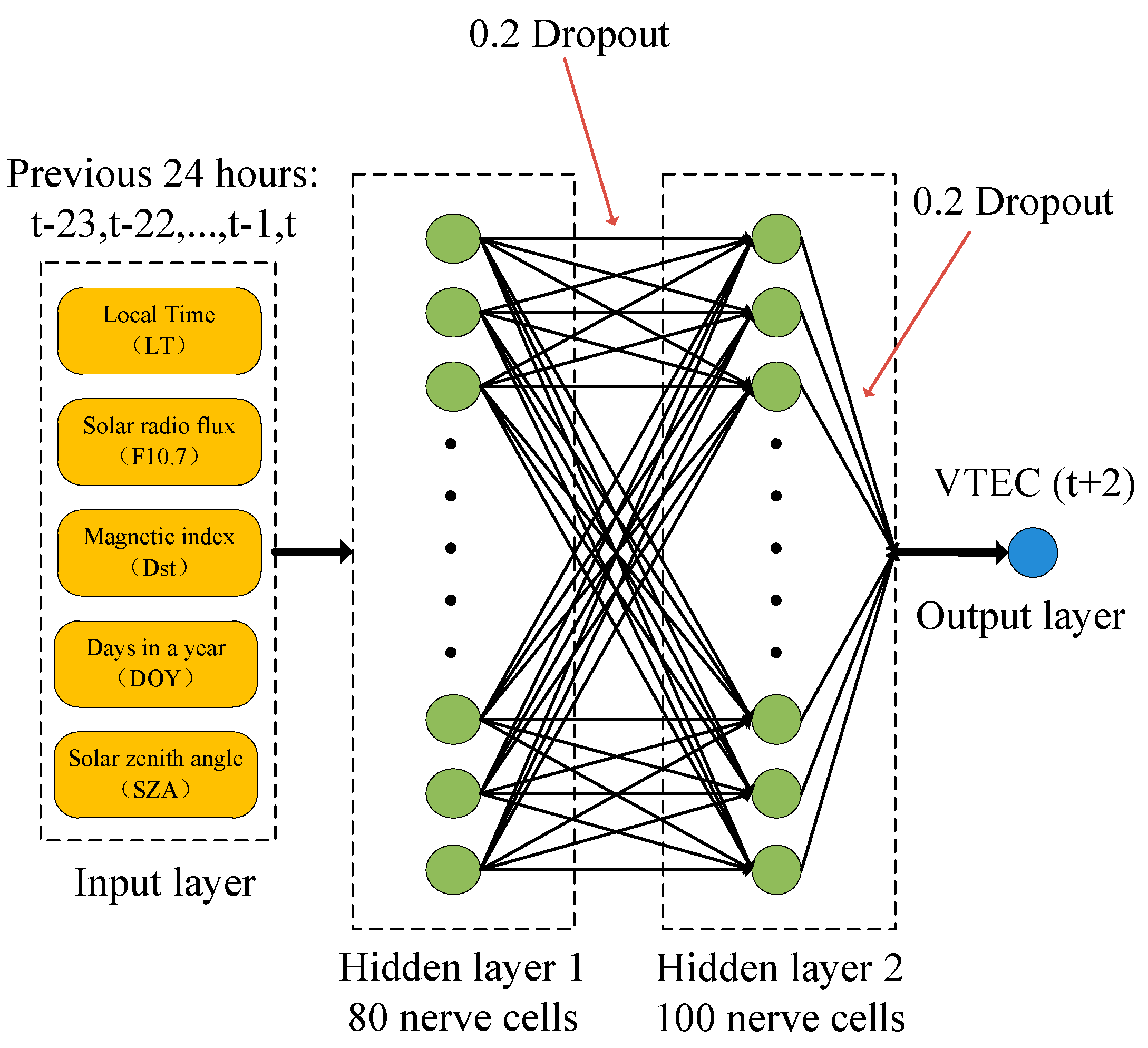
2.2.1. NN Model

The NN model input layer parameters were the local time (LT), F10.7, Dst, day of year (Doy), and solar zenith angle (SZA). There were 2 hidden layers in total, of which the number of neurons in the first hidden layer was 80, and the number of neurons in the second hidden layer was 100. Both layers used a 0.2 Dropout to suppress overfitting. The output layer was fully connected, and the density was set to 1 to predict the VTEC value. The network structure of the NN model is illustrated in Figure 3.

2.2.2. LSTM Model

To objectively compare the prediction of the ionospheric VTEC results of the NN model, the LSTM model input layer parameters, output layer parameters, number of hidden layers, and number of neurons in each hidden layer were made consistent with the NN model network structure. The hidden layer neurons were changed to LSTM neurons, and the structure of the LSTM model is shown in Figure 4.

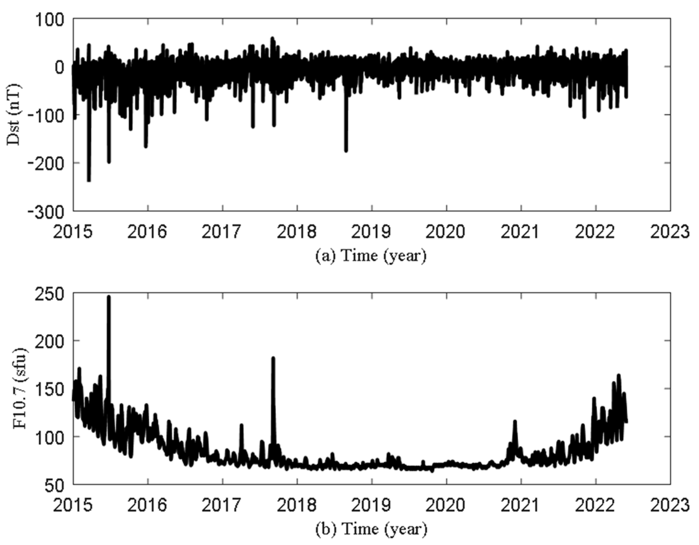
2.2.3. Database

Using the GNSS VTEC of the Haikou Station from January 2015 to May 2022, Figure 5 shows the hourly variation in the GNSS VTEC of Haikou Station in the 24th solar activity cycle decline stage and the 25th solar activity cycle rise stage. The hourly GNSS VTEC from 2015 to 2020 was used for training, the hourly GNSS VTEC from 2021 for validation, and the hourly GNSS VTEC from January to May 2022 for testing.

Dst (nT) and F10.7 (sfu) were provided by NASA (https://omniweb.gsfc.nasa.gov/) (accessed on 10 February 2023). It can be seen from Figure 6 that the geomagnetic disturbance in the falling phase of the 24th solar activity cycle is severe, and the geomagnetic disturbance in the rising phase of the 25th solar activity cycle is weak. F10.7 is consistent with the changing trend of the ionospheric VTEC at Haikou Station in Figure 5.

2.3. Accuracy Evaluation

To evaluate the results, the accuracy was calculated using RMSE, mean absolute error (MAE), and the correlation coefficient (R). Among them, RMSE and MAE represented the performance, while R represented the correlation between the observed values and the reference values.

$$\mathrm{RMSE}=\sqrt{\frac{1}{n}{\displaystyle \sum }_{i=1}^n{\left({\overline{y}}_i-y_i\right)}^2}$$

(20)

$$\mathrm{MAE}=\frac{1}{n}{\displaystyle \sum }_{i=1}^n\left|{\overline{y}}_i-y_i\right|$$

(21)

$$\mathrm{R}=\frac{\mathrm{cov}\left({\overline{y}}_i,y_i\right)}{{\sigma }_{{\overline{y}}_i}{\sigma }_{y_i}}$$

(22)

where $n$ is the total number of data samples; ${\overline{y}}_i$ and $y_i$ are the observed and reference values in the ionospheric VTEC estimation experiment; ${\overline{y}}_i$ and $y_i$ are the predicted and observed values in the ionospheric VTEC prediction experiment.

3. Results

3.1. Ionospheric VTEC Estimation Experiment

3.1.1. Site Observation Test in Non-Equatorial Anomaly Area

The Qingdao Station was selected to evaluate the accuracy of the proposed Kriging–Kalman method for estimating the GNSS VTEC (VTEC calculated using GNSS observing data) in a non-equatorial anomaly area. The internal coincidence accuracy (in

Table 1. Internal coincidence accuracy statistics of the proposed method to estimate the GNSS VTEC.

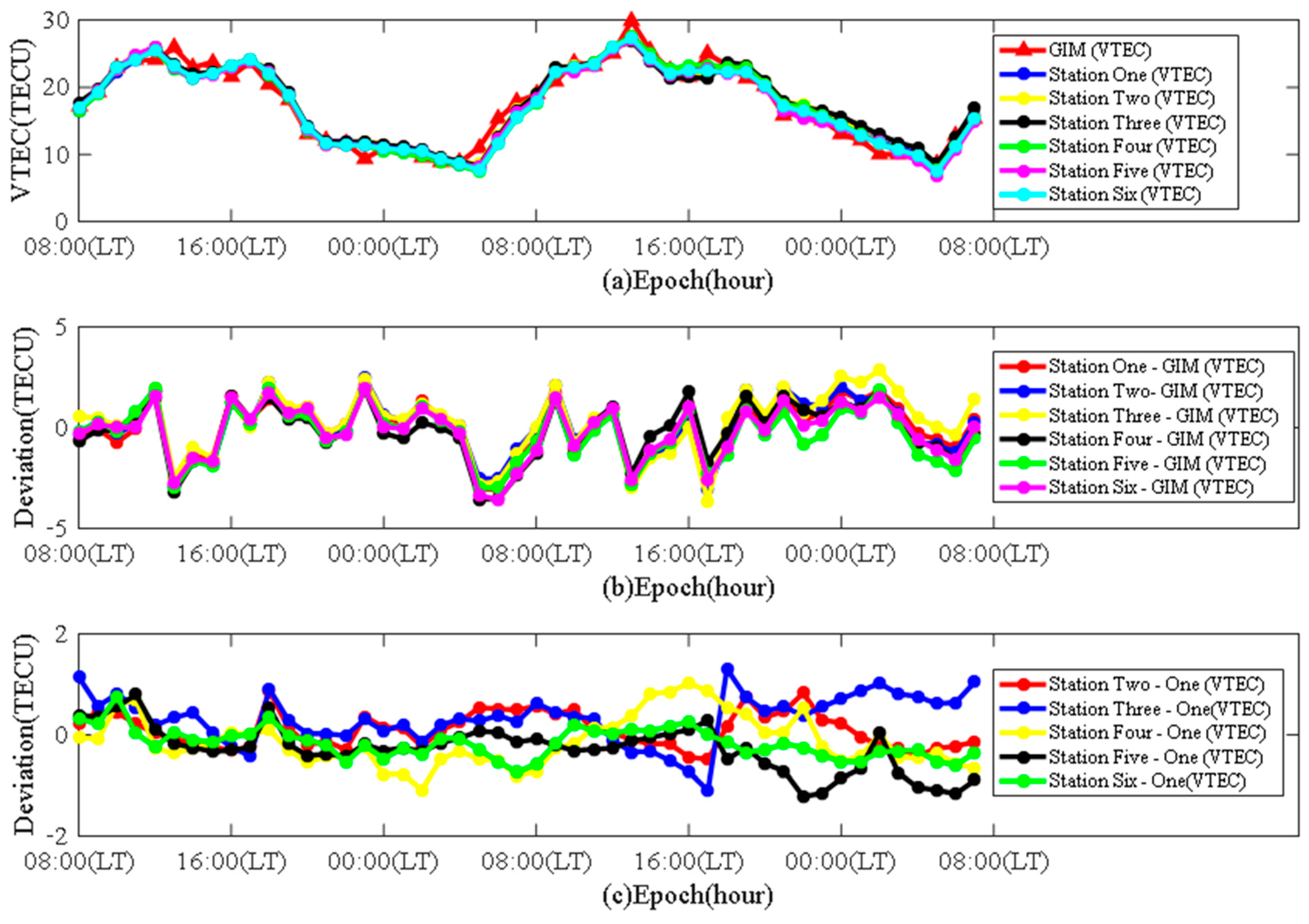
Station Numbers	RMSE (TECU)	MAE (TECU)	R
Two–One	0.3641	0.3015	0.9981
Three–One	0.5903	0.4917	0.9964
Four–One	0.5116	0.4248	0.9980
Five–One	0.5284	0.4079	0.9974
Six–One	0.3347	0.2681	0.9991
Statistics	0.4658	0.3788	0.9978

) of the proposed method for estimating the GNSS VTEC was verified using the same method with six GNSS observing equipment at the same site in Figure 7. The external coincidence accuracy (in

Table 2. External coincidence accuracy statistics of the proposed method to estimate the GNSS VTEC.

Station Number	RMSE (TECU)	MAE (TECU)	R
One	1.3577	1.0966	0.9731
Two	1.4211	1.1495	0.9705
Three	1.5612	1.2429	0.9659
Four	1.4021	1.1016	0.9721
Five	1.3803	1.1040	0.9733
Six	1.3731	1.0605	0.9728
Statistics	1.4159	1.1259	0.9713

) of the proposed method for estimating GNSS VTEC was then verified by comparison with the GIM VTEC results. Due to the different sampling rates of GNSS VTEC and GIM VTEC, the sampling rate of GNSS VTEC is 30 s and GIM VTEC is 1 h. GNSS VTEC was resampled at a sampling rate of 1 h (see Figure 8).

In the area of Qingdao Station, which is not affected by the equatorial anomaly, the GIM VTEC and GNSS VTEC obtained by the independent solution of the six GNSS observation at the same site exhibited a good consistency. The deviation between the GNSS VTEC and GIM VTEC was not affected by the daily variation peak of the ionospheric VTEC and did not change significantly during different times of the day. Deviation of the GNSS VTEC between different devices was less than the deviation between the GNSS VTEC and GIM VTEC. During the test, the maximum deviation of the GNSS VTEC between different devices within 1 day shall not exceed 1.31 TECU, and the consistency of the GNSS VTEC between different devices at all times was better than the GIM VTEC. These preliminary results showed that the Kriging–Kalman method can be used to estimate a high-precision GNSS VTEC in areas not affected by the equatorial anomaly.

3.1.2. Observation Experiment in Equatorial Anomaly Area

Haikou Station (110.34°E, 20.00°N), which is located in the equatorial anomaly area, was selected as the test site to verify the accuracy of the proposed Kriging–Kalman method for estimating the ionospheric VTEC in the equatorial anomaly region (see Figure 9). By comparison with the results of the GIM VTEC, it was noted that the results provided by the GIM VTEC during the equatorial anomaly period have a large deviation; therefore, this study proposed the additional method for verifying the accuracy of the ionospheric VTEC during the equatorial anomaly period.

In order to prove that Haikou Station is within the equatorial anomaly area, Figure 10a–c shows the background ionospheric VTEC of Haikou and Qingdao with different local times during the occurrence of the equatorial anomaly. The GIM VTEC used GNSS observation data provided by global GNSS observation stations to obtain a spherical harmonic function model. To describe the daily variation trend of the ionospheric VTEC, the typical method is to estimate a group of spherical harmonic coefficients every 2 h during a single day. In this study, considering the continuity of the ionospheric VTEC variation between adjacent days, the GIM VTEC of the middle day was calculated using 3-day observation data [36,37]. Figure 10d shows the change results of the GIM VTEC with latitudes at the times of 08, 12, 14, 16, 18, and 22 (LT) along the longitude line of 110.34°E.

It could be seen from Figure 10a–c that Haikou is in the equatorial anomaly area, while Qingdao is in the non-equatorial anomaly area. It could be seen from Figure 10d that the deviation between the GIM VTEC and GNSS VTEC at Haikou Station is relatively large during the period from 12 (LT) to 17 (LT), and the results showed good agreement in other periods. From the change of the GIM VTEC along the longitude line of 110.34°E with the latitude at different times, it can be seen that the occurrence time of equatorial anomaly in the northern hemisphere coincides with the period of large deviation between the GIM VTEC and GNSS VTEC.

To further explain the large deviation of the GIM VTEC in the equatorial anomaly, the third Geostationary Earth Orbit (GEO3) satellite of Beidou Navigation Satellite System (BDS), which is closest to Haikou Station, was selected for verification (the coordinates of the sub-satellite point were 18.54°N and 110.37°E). The shared position of the GEO satellite and GNSS receiver was relatively static, resulting in the high accuracy of the GEO satellite phase TEC data; meanwhile, the GEO satellite phase TEC data were consistent with the true value deviation constant (DCB) in the short term. Considering that the GIM VTEC and GNSS VTEC coincided well in the 02 (LT) to 06 (LT) period, the GIM VTEC of that period were used to calibrate the deviation of the BDS GEO3 VTEC and obtain high-precision ionospheric VTEC results over Haikou Station.

As shown in Figure 11, Haikou Station was affected by the equatorial anomaly, resulting in a maximum deviation of 10 TECU between the GIM VTEC and GNSS VTEC. The analysis revealed that this deviation was caused by the weakening of the expression ability of the spherical harmonic function model adopted by the GIM in the equatorial anomaly region. The accuracy of the proposed Kriging–Kalman method for estimating the ionospheric VTEC in the equatorial anomaly area was verified using the TEC projection of the GEO satellite phase closest to Haikou Station and the calibration method of the GIM VTEC in the non-equatorial anomaly influence period. It can be seen from

Table 3. Precision Statistical Results of the GNSS VTEC, GIM VTEC and BDS GEO3 VTEC at Haikou Station.

Deviation	RMSE (TECU)	MAE (TECU)	R
GNSS (VTEC)-GIM (VTEC)	3.7713	2.7388	0.9870
GNSS (VTEC)-BDS GEO3 (VTEC)	1.9204	1.5553	0.9942

that the estimated ionospheric VTEC RMSE result of the proposed method in the equatorial anomaly area was 1.9204 TECU, the MAE result was 1.5553 TEC, and the R result was 0.9942, which was equivalent to the estimated ionospheric VTEC result of Qingdao Station in the non-equatorial anomaly area.

3.2. Ionospheric VTEC Prediction Experiment

The LSTM and NN models were used to train the database data. The optimizer selected was Adam, and the loss function selected was the mean squared error, batch size = 128, and epoch = 50. The prediction accuracy of the VTEC in the equatorial anomaly region with different prediction times in the LSTM and NN models from January to May 2022 was analyzed and compared with the prediction results of the IRI2016. The specific results are shown in Figure 12, Figure 13, Figure 14 and Figure 15 and

Table 4. Forecast accuracy of the LSTM model VTEC and NN model VTEC.

Forecast Duration (h)	LSTM Model			NN Model
	RMSE (TECU)	MAE (TECU)	R	RMSE (TECU)	MAE (TECU)	R
1	2.4636	1.7886	0.9948	6.8740	4.8839	0.9940
2	4.5672	3.3162	0.9862	7.8217	5.5972	0.9859
4	5.5284	4.0286	0.9737	8.7482	6.1541	0.9738
>8	6.2093	4.4957	0.9666	9.4552	6.5320	0.9648

.

Figure 12 and Figure 13 show the distributions of the ionospheric VTEC prediction errors of the LSTM and NN models for different prediction durations. As shown in Figure 12, the mean value of the ionospheric VTEC prediction error of the LSTM model for different prediction durations was approximately 0, indicating that the results of the LSTM model for predicting the ionospheric VTEC were unbiased estimates. As shown in Figure 13, the mean value of the ionospheric VTEC prediction error of the NN model was less than 0 for different prediction durations, indicating that the results of the ionospheric VTEC prediction by the NN model were biased estimates. Figure 14 and Figure 15 showed the correlation between the LSTM and NN model ionospheric VTEC predicted values and the observed values for different forecast durations. The correlation between the LSTM model and the NN model ionospheric VTEC predicted value and the observed value for different forecast durations was very high, which was consistent with the R results listed in Table 4, and the correlation gradually decreased with increasing forecast duration.

Table 4 presented the statistical results of the ionospheric VTEC prediction accuracies of the LSTM and NN models for different prediction durations. The ionospheric VTEC prediction accuracy of the LSTM model for the different prediction durations was higher than that of the NN model. Even when the forecast duration of the LSTM model exceeded 8 h, the prediction accuracy of the ionospheric VTEC was still better than that of the NN model by 1 h. The prediction accuracy of the one hour LSTM model ionospheric VTEC was significantly better than that of the other prediction durations. The improvement rate of the ionospheric VTEC prediction accuracy increased with a reduction in the prediction duration; in particular, the prediction accuracy of the one hour ionospheric VTEC was 46.06% higher than the two hour prediction duration. The IRI2016 was used to predict the ionospheric VTEC RMSE result of Haikou Station, which was 15.3502 TECU, MAE was 11.7394 TECU, and R was 0.9095, the values of which were lower than those of the LSTM and NN models in the prediction accuracy of the ionospheric VTEC.

The periods from 21–23 February and 9–11 April 2022, where the equatorial anomaly was relatively significant, were selected for further analysis. Figure 16 shows a comparison of the LSTM, NN, and IRI2016 ionospheric VTEC prediction and observation results.

According to the analysis of the occurrence time of the ionospheric equatorial anomaly predicted by the different models, the peak of the daily variation of the ionospheric VTEC differed in different months, and the peak of the daily variation of the ionospheric VTEC in April 2022 was later than that in February 2022. Compared to IRI2016, the LSTM and NN models accurately predicted the occurrence time of the ionospheric equatorial anomaly. This was consistent with the conclusion of the LSTM model R and NN model R in Table 4, and was superior to IRI2016 R. This indicateed that the LSTM and NN models can accurately predict the occurrence time of an equatorial anomaly.

4. Discussion

While many studies have investigated methods for estimating [16,17,18,19,20] and forecasting the ionospheric VTEC [23,24,25,26,27,28,29,30,31,32] based on GNSS observing data, very little work has been done on using Long term GNSS observation data from an equatorial ionization anomaly region for high precision estimation and prediction of the ionospheric VTEC. Two experiments were carried out in this study.

Experiment 1 evaluated the accuracy of the Kriging–Kalman method for estimating the ionospheric VTEC, which was achieved by improving the Kalman method, a high-precision method for estimating the ionospheric TEC in the equatorial anomaly area. The Kriging–Kalman method was thus proposed. In addition, a method was proposed for verifying the accuracy of the ionospheric VTEC during the occurrence of an equatorial anomaly. The accuracy of the Kriging–Kalman method for estimating the ionospheric VTEC was verified using observational data from the Qingdao and Haikou stations. It can be seen from Table 2 and Table 3 that using the Kriging–Kalman method to estimate the ionospheric VTEC at Qingdao and Haikou stations can obtain almost the same accuracy.

Experiment 2 analyzed and compared the accuracy of the ionospheric VTEC prediction by different models during the equatorial anomaly period at Haikou Station, using the long-term GNSS VTEC of Haikou Station through training of the NN and LSTM, and compared the accuracy of the IRI, NN, and LSTM models for the equatorial anomaly period and ionospheric TEC prediction. From the analysis of the ionospheric VTEC prediction accuracy, the LSTM model was found to be more accurate than the other two models, especially the 1 h prediction results. The LSTM model prediction results were consistent with the GNSS VTEC at all time periods in the day, indicating that the LSTM model can predict the ionospheric VTEC changes with high accuracy during the equatorial anomaly. For the NN model, the ionospheric VTEC prediction results were smaller than the observation results at the time of the equatorial anomaly, which was consistent with the mean value of the ionospheric VTEC prediction error that was shown in Figure 13, which was less than 0.

5. Conclusions

This study introduced the proposed Kriging–Kalman method to estimate the ionospheric VTEC and verified the method’s observation accuracy of the GNSS VTEC in the non-equatorial anomaly region of Qingdao using multiple equipment and site observations. The external conformity accuracy with the GIM VTEC was RMSE = 1.42 TECU and R = 0.9713, and the internal conformity accuracy between instruments was RMSE = 0.4658 TECU and R = 0.9978. A method for evaluating the accuracy of the GNSS VTEC in equatorial anomaly areas has been proposed. High-precision phase TEC observation data from the closest satellite to Haikou Station, BDS3, were selected to verify the accuracy of the proposed method for the GNSS VTEC versus BDS GEO3 VTEC in that region; the results were RMSE = 1.92 TECU and R = 0.9942. From the above, it can be seen that the Kriging–Kalman method can effectively estimate the ionospheric VTEC in the equatorial anomaly areas.

Based on the GNSS VTEC of Haikou Station, F10.7, Dst, and other data, the prediction accuracy of the VTEC in the ionosphere with different prediction times in the equatorial anomaly region of the LSTM and NN models was analyzed and compared with the prediction results of the IRI. The NN model could accurately predict the time of occurrence of an ionospheric VTEC equatorial anomaly. The LSTM model could accurately predict the occurrence time of the ionospheric VTEC equatorial anomaly and accurately reflect the ionospheric VTEC changes during the equatorial anomaly period. The prediction accuracy of the LSTM model for different prediction periods was better than that of the NN and IRI models.

References

- Jin, S.; Jin, R.; Li, D. GPS detection of ionospheric Rayleigh wave and its source following the 2012 Haida Gwaii earthquake. J. Geophys. Res. Space Phys. 2017, 122, 1360–1372. [Google Scholar] [CrossRef]
- Jin, S. Two-Mode Ionospheric Disturbances Following the 2005 Northern California Offshore Earthquake from GPS Measurements. J. Geophys. Res. Space Phys. 2018, 123, 8587–8598. [Google Scholar] [CrossRef]
- Goodman, J.M. Operational communication systems and relationships to the ionosphere and space weather. Adv. Space Res. 2005, 36, 2241–2252. [Google Scholar] [CrossRef]
- Ritchie, S.E.; Honary, F. Storm sudden commencement and its effect on high-latitude HF communication links. Space Weather 2009, 7, S06005. [Google Scholar] [CrossRef] [Green Version]
- Deng, Y.; Ridley, A.J. The Global Ionosphere-Thermosphere Model and the Nonhydrostatic Processes. Geophys. Monogr. Ser. 2014, 201, 85–100. [Google Scholar] [CrossRef]
- Chetia, B.; Barman, M.K.; Devi, M.; Barbara, A.K. Study of Physical and Dynamical Processes in the Ionosphere at Equatorial Anomaly Crest Region during Magnetic Storm for High and Low Solar Activity Period. In Geostatistical and Geospatial Approaches for the Characterization of Natural Resources in the Environment; Springer: Berlin/Heidelberg, Germany, 2016; pp. 861–866. [Google Scholar] [CrossRef]
- Kouris, S.S.; Xenos, T.D.; Polimeris, K.V.; Stergiou, D. TEC and foF2 variations: Preliminary results. Ann. Geophys. 2009, 47, 1325–1332. [Google Scholar] [CrossRef]
- Gowtam, V.S.; Ram, S.T. Ionospheric annual anomaly-New insights to the physical mechanisms. J. Geophys. Res. Space Phys. 2017, 122, 8816–8830. [Google Scholar] [CrossRef]
- Balan, N.; Liu, L.; Le, H. A brief review of equatorial ionization anomaly and ionospheric irregularities. Earth Planet. Phys. 2018, 2, 257–275. [Google Scholar] [CrossRef]
- Gan, Q.; Wang, W.; Yue, J.; Liu, H.; Chang, L.C.; Zhang, S.; Burns, A.; Du, J. Numerical simulation of the 6 day wave effects on the ionosphere: Dynamo modulation. J. Geophys. Res. Space Phys. 2016, 121, 10103–10116. [Google Scholar] [CrossRef]
- Ferdousi, B.; Raeder, J. Signal propagation time from the magnetotail to the ionosphere: OpenGGCM simulation. J. Geophys. Res. Space Phys. 2016, 121, 6549–6561. [Google Scholar] [CrossRef]
- Ridley, A.J.; Deng, Y.; Tóth, G. The global ionosphere–thermosphere model. J. Atmos. So-Lar-Terr. Phys. 2006, 68, 839–864. [Google Scholar] [CrossRef]
- Bilitza, D.; Altadill, D.; Truhlik, V.; Shubin, V.; Galkin, I.; Reinisch, B.; Huang, X. International Reference Ionosphere 2016: From ionospheric climate to real-time weather predictions. Space Weather 2017, 15, 418–429. [Google Scholar] [CrossRef]
- Wang, N.; Li, Z.; Yuan, Y.; Li, M.; Huo, X.; Yuan, C. Ionospheric correction using GPS Klobuchar coefficients with an empirical night-time delay model. Adv. Space Res. 2018, 63, 886–896. [Google Scholar] [CrossRef]
- Jiang, H.; Liu, J.; Wang, Z.; An, J.; Ou, J.; Liu, S.; Wang, N. Assessment of spatial and temporal TEC variations derived from ionospheric models over the polar regions. J. Geod. 2019, 93, 455–471. [Google Scholar] [CrossRef]
- Sardón, E.; Rius, A.; Zarraoa, N. Estimation of the transmitter and receiver differential biases and the ionospheric total electron content from Global Positioning System observations. Radio Sci. 1994, 29, 577–586. [Google Scholar] [CrossRef]
- Ma, G.; Gao, W.; Li, J.; Chen, Y.; Shen, H. Estimation of GPS instrumental biases from small scale network. Adv. Space Res. 2014, 54, 871–882. [Google Scholar] [CrossRef]
- Chen, L.; Yi, W.; Song, W.; Shi, C.; Lou, Y.; Cao, C. Evaluation of three ionospheric delay computation methods for ground-based GNSS receivers. GPS Solut. 2018, 22, 125. [Google Scholar] [CrossRef]
- Lu, W.; Ma, G.; Wang, X.; Wan, Q.; Li, J. Evaluation of ionospheric height assumption for single station GPS-TEC der-ivation. Adv. Space Res. 2017, 60, 286–294. [Google Scholar] [CrossRef]
- Cai, H.; Wang, Q. Resolving the Regional Ionospheric Grid Model by Applying Kalman Filter. China Satell. Navig. Conf. 2016, 390, 425–434. [Google Scholar] [CrossRef]
- Prasad, R.; Kumar, S.; Jayachandran, P. Receiver DCB estimation and GPS vTEC study at a low latitude station in the South Pacific. J. Atmos. Sol. -Terr. Phys. 2016, 149, 120–130. [Google Scholar] [CrossRef]
- Zhang, Q.; Zhao, Q.L. Evaluation and analysis of the global ionosphere maps from Wuhan University IGS Ionosphere Associate Analysis Center. Chin. J. Geophys. 2019, 62, 4493–4505. (In Chinese) [Google Scholar]
- Tulunay, E.; Senalp, E.T.; Radicella, S.M.; Tulunay, Y. Forecasting total electron content maps by neural network technique. Radio Sci. 2006, 41, RS4016. [Google Scholar] [CrossRef]
- Dabbakuti, J.K.; Ratnam, D.V. Performance evaluation of linear time-series ionospheric Total Electron Content model over low latitude Indian GPS stations. Adv. Space Res. 2017, 60, 1777–1786. [Google Scholar] [CrossRef]
- Li, W.; Zhao, D.; Shen, Y.; Zhang, K. Modeling Australian TEC Maps Using Long-Term Observations of Australian Regional GPS Network by Artificial Neural Network-Aided Spherical Cap Harmonic Analysis Approach. Remote Sens. 2020, 12, 3851. [Google Scholar] [CrossRef]
- Adolfs, M.; Hoque, M.M. A Neural Network-Based TEC Model Capable of Reproducing Nighttime Winter Anomaly. Remote Sens. 2021, 13, 4559. [Google Scholar] [CrossRef]
- Adolfs, M.; Hoque, M.M.; Shprits, Y.Y. Storm-Time Relative Total Electron Content Modelling Using Machine Learning Techniques. Remote Sens. 2022, 14, 6155. [Google Scholar] [CrossRef]
- Lin, X.; Wang, H.; Zhang, Q.; Yao, C.; Chen, C.; Cheng, L.; Li, Z. A Spatiotemporal Network Model for Global Ionospheric TEC Forecasting. Remote Sens. 2022, 14, 1717. [Google Scholar] [CrossRef]
- Tang, J.; Li, Y.; Ding, M.; Liu, H.; Yang, D.; Wu, X. An Ionospheric TEC Forecasting Model Based on a CNN-LSTM-Attention Mechanism Neural Network. Remote Sens. 2022, 14, 2433. [Google Scholar] [CrossRef]
- Kim, J.-H. Potential of Regional Ionosphere Prediction Using a Long Short-Term Memory Deep-Learning. Space Weather 2021, 19, e2021SW002741. [Google Scholar] [CrossRef]
- Ren, X.; Yang, P.; Liu, H.; Chen, J.; Liu, W. Deep Learning for Global Ionospheric TEC Forecasting: Different Approaches and Validation. Space Weather 2022, 20, e2021SW003011. [Google Scholar] [CrossRef]
- Ulukavak, M. Deep learning for ionospheric TEC forecasting at mid-latitude stations in Turkey. Acta Geophys. 2021, 69, 589–606. [Google Scholar] [CrossRef]
- Oliver, M.A.; Webster, R. Kriging: A method of interpolation for geographical information systems. Int. J. Geogr. Inf. Syst. 1990, 4, 313–332. [Google Scholar] [CrossRef]
- Cortesi, A.F.; Jannoun, G.; Congedo, P.M. Kriging-sparse Polynomial Dimensional Decomposition surrogate model with adaptive refinement. J. Comput. Phys. 2018, 380, 212–242. [Google Scholar] [CrossRef] [Green Version]
- Imran, M.; Stein, A.; Zurita-Milla, R. Using geographically weighted regression kriging for crop yield mapping in West Africa. Int. J. Geogr. Inf. Sci. 2014, 29, 234–257. [Google Scholar] [CrossRef]
- Liu, C.; Liu, C.; Feng, X.; Quan, W. Quality Evaluation of IGS GIMs Based on the Statistical Characteristics of VTEC/RMS Eigenvalues: A Macro Perspective. Radio Sci. 2018, 53, 790–803. [Google Scholar] [CrossRef]
- Jee, G.; Lee, H.-B.; Kim, Y.H.; Chung, J.-K.; Cho, J. Assessment of GPS global ionosphere maps (GIM) by comparison between CODE GIM and TOPEX/Jason TEC data: Ionospheric perspective. J. Geophys. Res. Space Phys. 2010, 115, A10319. [Google Scholar] [CrossRef] [Green Version]