
A Benchmark for Multi-Modal LiDAR SLAM with Ground Truth in GNSS-Denied Environments
by
 , , , , and
Ha Sier
1,2,† ,
,
Qingqing Li
2,†,
Xianjia Yu
2,*,
Jorge Peña Queralta
2,
Zhuo Zou
1,† and
Tomi Westerlund
2
1
School of Information Science and Technology, Fudan University, Shanghai 200433, China
2
Turku Intelligent Embedded and Robotic Systems Lab, Faculty of Technology, University of Turku, 20014 Turuku, Finland
*
Author to whom correspondence should be addressed.
†
These authors contributed equally to this work.
Remote Sens. 2023, 15(13), 3314; https://doi.org/10.3390/rs15133314
Submission received: 3 May 2023
/
Revised: 16 June 2023
/
Accepted: 21 June 2023
/
Published: 28 June 2023
Abstract
:LiDAR-based simultaneous localization and mapping (SLAM) approaches have obtained considerable success in autonomous robotic systems. This is in part owing to the high accuracy of robust SLAM algorithms and the emergence of new and lower-cost LiDAR products. This study benchmarks the current state-of-the-art LiDAR SLAM algorithms with a multi-modal LiDAR sensor setup, showcasing diverse scanning modalities (spinning and solid state) and sensing technologies, and LiDAR cameras, mounted on a mobile sensing and computing platform. We extend our previous multi-modal multi-LiDAR dataset with additional sequences and new sources of ground truth data. Specifically, we propose a new multi-modal multi-LiDAR SLAM-assisted and ICP-based sensor fusion method for generating ground truth maps. With these maps, we then match real-time point cloud data using a normal distributions transform (NDT) method to obtain the ground truth with a full six-degrees-of-freedom (DOF) pose estimation. These novel ground truth data leverage high-resolution spinning and solid-state LiDARs. We also include new open road sequences with GNSS-RTK data and additional indoor sequences with motion capture (MOCAP) ground truth, complementing the previous forest sequences with MOCAP data. We perform an analysis of the positioning accuracy achieved, comprising ten unique configurations generated by pairing five distinct LiDAR sensors with five SLAM algorithms, to critically compare and assess their respective performance characteristics. We also report the resource utilization in four different computational platforms and a total of five settings (Intel and Jetson ARM CPUs). Our experimental results show that the current state-of-the-art LiDAR SLAM algorithms perform very differently for different types of sensors. More results, code, and the dataset can be found at GitHub.
1. Introduction
LiDAR sensors have been adopted as the core perception sensor in many applications, from self-driving cars [1] to unmanned aerial vehicles [2], including forest surveying and industrial digital twins [3]. High-resolution spinning LiDARs enable a high degree of awareness of the surrounding environments. More dense 3D point clouds and maps are in increasing demand to support the next wave of ubiquitous autonomous systems as well as more detailed digital twins across industries. However, higher angular resolution comes at an increased cost in analog LiDARs, requiring a higher number of laser beams or a more compact electronics and optics solution. New solid-state and other digital LiDARs are paving the way to cheaper and more widespread 3D LiDAR sensors capable of dense environment mapping [4,5,6,7].
So-called solid-state LiDARs overcome some of the challenges of spinning LiDARs in terms of cost and resolution but introduce some new limitations in terms of a relatively small field of view (FoV) [6,8]. Indeed, these LiDARs provide a greater sensing range at a significantly lower cost [9]. Other limitations that affect traditional approaches to LiDAR data processing include irregular scanning patterns or increased motion blur.
Despite their increasing popularity, few works have benchmarked the performance of both spinning LiDAR and solid-state LiDAR in diverse environments, which limits the development of more general-purpose LiDAR-based SLAM algorithms [9]. To bridge the gap in the literature, we present a benchmark that compares different modality LiDARs (spinning, solid state) in diverse environments, including offices, long corridors, halls, forests, and open roads. To allow for a more accurate and fair comparison, we introduce a new method for ground truth generation in larger indoor spaces (see Figure 1). This enhanced ground truth enables a significantly higher degree of quantitative benchmarking and comparison with respect to our previous work [9]. We hope for the extended dataset and ground truth labels, as well as more detailed data, to provide a performance reference for multi-modal LiDAR sensors in both structured and unstructured environments to both academia and industry.
In summary, this work evaluates state-of-the-art SLAM algorithms with a multi-modal multi-LiDAR platform as an extension of our previous work [9]. The main contributions of this work are as follows:
- 1.
- A ground truth trajectory generation method for environments where MOCAP or GNSS/RTK are unavailable. The method leverages the multi-modality of the data acquisition platform and high-resolution sensors;
- 2.
- A new dataset composed of data from five different LiDAR sensors, one LiDAR camera, and one stereo fisheye camera (see Figure 2) in various environments. Ground truth data are provided for all sequences;
- 3.
- The benchmarking of ten state-of-the-art filter-based and optimization-based SLAM methods on our proposed dataset in terms of the accuracy of odometry, memory, and computing resource consumption. The results indicate the limitations of the current SLAM algorithms and potential future research directions.
The structure of this paper is as follows. Section 2 surveys the recent progress in SLAM and existing LiDAR-based SLAM benchmarks. Section 3 provides an overview of the configuration of the proposed sensor system. Section 4 offers the detailed benchmark and ground truth generation methodology. Section 5 concludes the study and suggests future work.
2. Related Works
Owing to high accuracy, versatility, and resilience across environments, 3D LiDAR SLAM has been studied as a crucial component of robotic and autonomous systems [10]. In this section, we limit the scope to the well-known and well-tested 3D LiDAR SLAM methods. We also include an overview of the most recent 3D LiDAR SLAM benchmarks.
2.1. Three-Dimensional LiDAR SLAM
The primary types of 3D LiDAR SLAM algorithms today are LiDAR only [11] and loosely coupled [12] or tightly coupled [13] with IMU data. Tightly coupled approaches integrate the LiDAR and IMU data at an early stage, in opposition to SLAM methods that loosely fuse the LiDAR and IMU outputs toward the end of their respective processing pipelines.
In terms of LiDAR-only methods, an early work by Zhang et al. on LiDAR odometry and mapping (LOAM) introduced a method that can already achieve low drift and low-computational complexity in 2014 [14]. Since then, there have been multiple variations of LOAM that enhance its performance. By incorporating ground point segmentation and a loop closure module, LeGO-LOAM is more lightweight with the same accuracy but improved computational expense and lower long-term drift [15]. However, LiDAR-only approaches are mainly limited by high susceptibility to featureless landscapes [16,17]. By incorporating IMU data into the state estimation pipeline, SLAM systems naturally become more precise and flexible.
In LIOM [13], the authors proposed a novel tightly coupled approach with LiDAR-IMU fusion based on graph optimization which outperformed the state-of-the-art LiDAR-only and loosely coupled methods. Owing to the better performance of tightly coupled approaches, subsequent studies have focused on this direction. Another practical tightly coupled method is Fast-LIO [18], which provides computational efficiency and robustness by fusing the feature points with IMU data through an iterated extended Kalman filter. By extending FAST-LIO, FAST-LIO2 [19] integrated a dynamic structure ikd-tree to the system that allows for the incremental map update at every step, addressing computational scalability issues while inheriting the tightly coupled fusion framework from FAST-LIO.
The vast majority of these algorithms function well with spinning LiDARs. Nonetheless, new approaches are in demand because from new sensors such as solid-state Livox LiDARs, novel sensing modalities, smaller FoVs, and irregular samplings have emerged [9]. Multiple existing studies using enhanced SLAM algorithms are being researched to fit these new LiDAR characteristics. Loam livox [8] is a robust and real-time LOAM algorithm for these types of LiDARs. LiLi-OM [6] is another tightly coupled method that jointly minimizes the cost derived from LiDAR and IMU measurements for both solid-state LiDARs and conventional LiDARs.
2.2. SLAM Benchmarks
There are various multi-sensor datasets available online. We had a systematic comparison of the popular datasets in our former work [9]. Among these datasets, not all of them have an analytical benchmark of 3D LiDAR SLAM based on multi-modality LiDARs. The KITTI benchmark [22] is the most significant one with the capability of evaluating several tasks, including, for example, odometry, SLAM, object detection, and tracking.
3. Data Collection
Our data collection platform is shown in Figure 2, and the details of the sensors are listed in Table 1. The platform is mounted on a mobile-wheeled vehicle to adapt to varying environments. In most scenarios, the platform is manually pushed or teleoperated, except for the forest environment where the platform is handheld.
3.1. Data Collection Platform
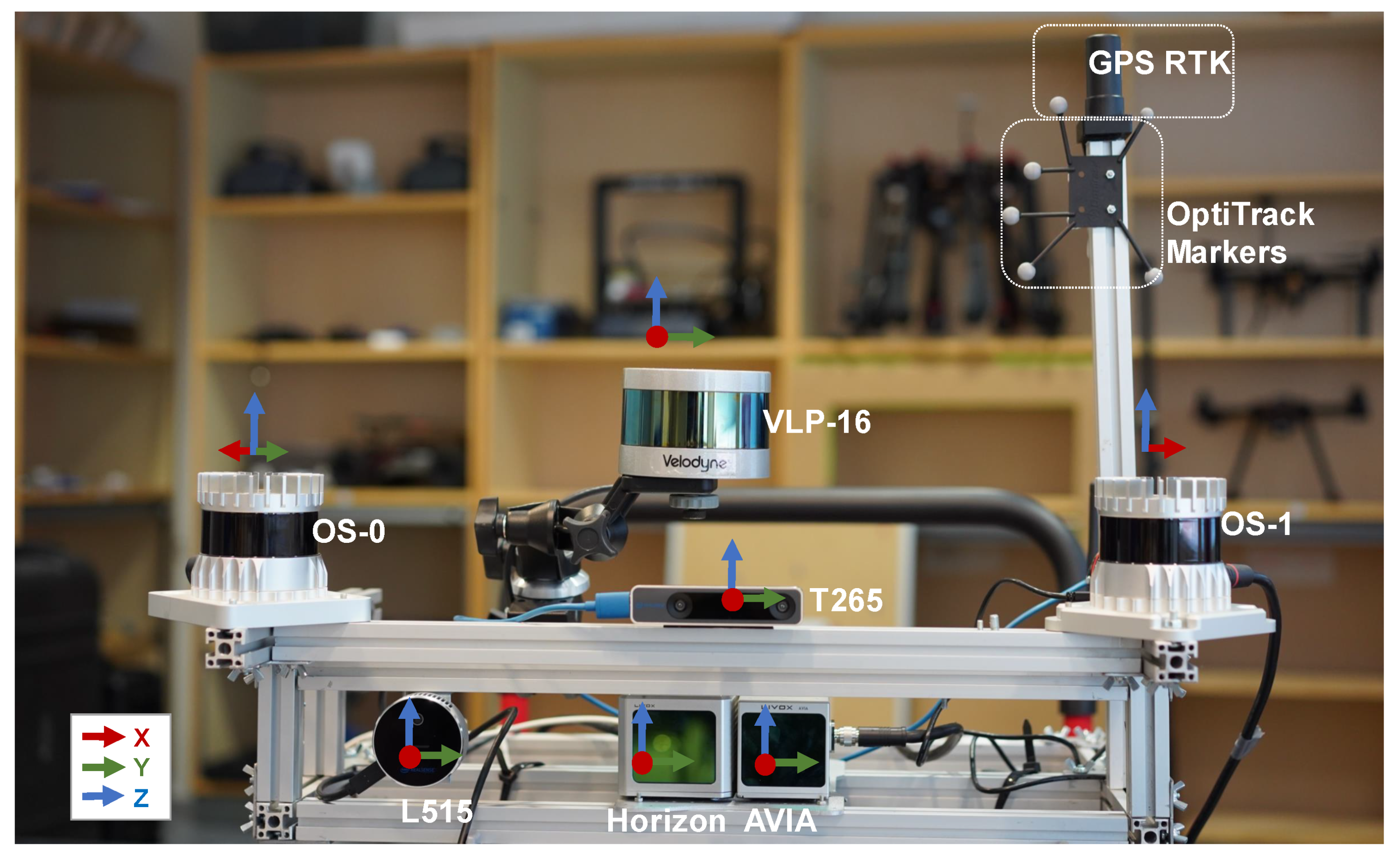
The data collection platform contains various LiDAR sensors, from traditional spinning LiDARs with different resolutions to novel solid-state LiDAR featured with non-repetition scanning patterns. A LiDAR camera and stereo fisheye camera are also included. There are three spinning LiDARs: a 16-channel Velodyne LiDAR (VLP-16), a 64-channel Ouster LiDAR (OS1), and a 128-channel Ouster LiDAR (OS0). The OS0 and OS1 sensors are mounted on the left and right sides, where the OS1 is turned 45 degrees clockwise, and the OS0 is turned 45 degrees anticlockwise. The Velodyne LiDAR is at the top-most position. Two solid-state LiDARs, Horizon and Avia, are installed in the center of the frame. The Optitrack marker set for the MOCAP-based and the antenna for the GNSS/RTK ground truth are both fixed on the top of the aluminum stick to maximize its visibility and detection range. All sensors are connected to a computer, featuring an Intel i7-10750h processor, 64 GB of DDR4 RAM memory, and 1 TB SSD storage, through a Gigabit Ethernet router. The data collection system, including sensor drivers and online calibration scripts, are running on ROS Melodic under Ubuntu 18.04 owing entirely to the wider variety of ROS-based LiDAR SLAM methods available for Melodic.
3.2. Calibration and Synchronization
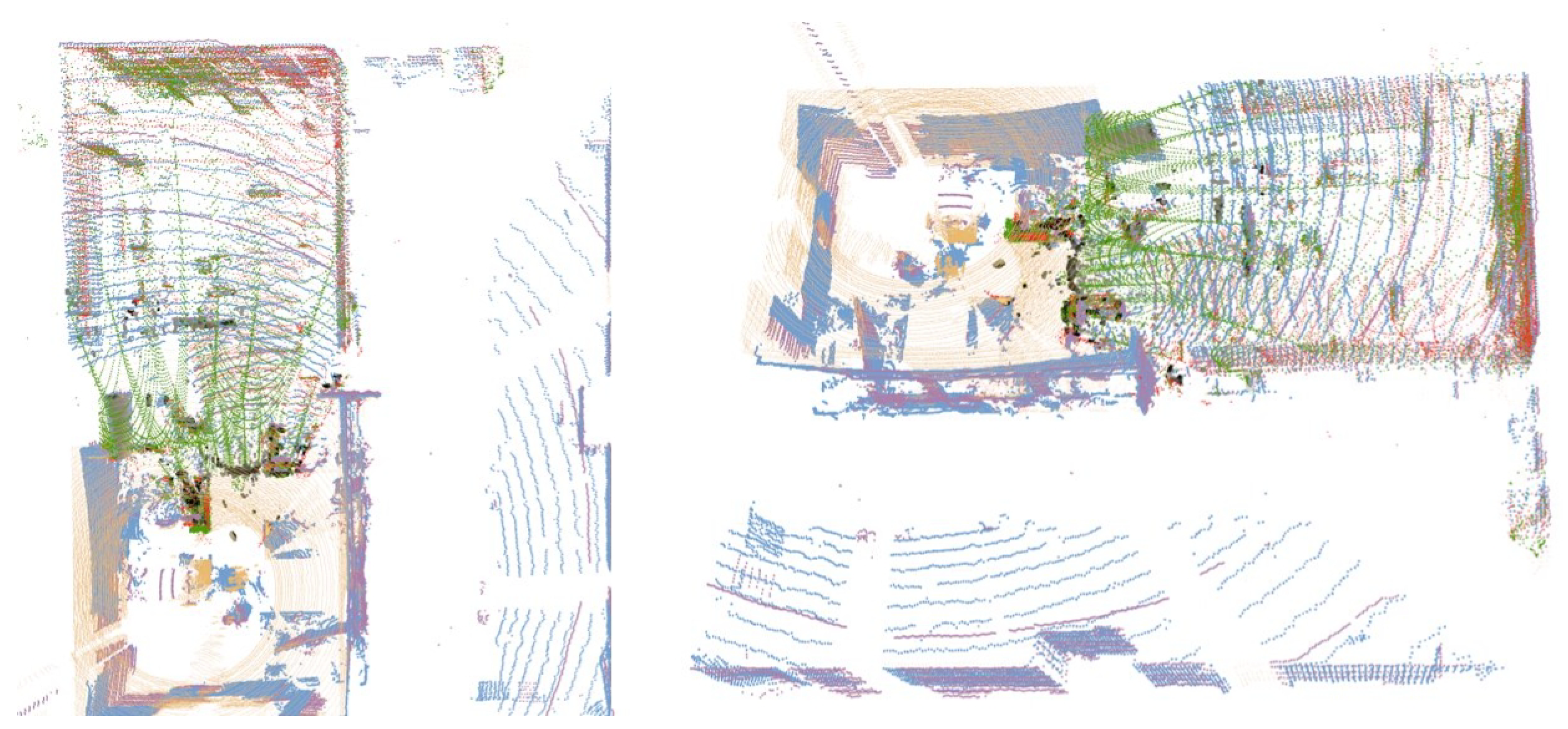
Efficient extrinsic parameters calibration is crucial to multi-sensor platforms, especially for handmade devices where the extrinsic parameters may change due to unstable connections or distortion of the material during transit. Similar to our previous work [9], we calculate the extrinsic parameter of sensors before each data collecting process. Figure 3 shows the calibration result of sample LiDAR data from one of the indoor data sequences.
Different to our previous work [9], where the timestamps of Ouster and Livox LiDARs are kept based on their own clock, we synchronize all LiDAR sensors in ethernet mode via the software-based precise timestamp protocol (PTP) [23]. We compare the orientation estimation between the sensor’s built IMUs and SLAM results with LiDARs and conclude that the latency of our system is below 5 ms.
3.3. SLAM-Assisted Ground Truth Map
To provide accurate ground truth for large-scale indoor and outdoor environments, where the MOCAP system is unavailable or the GNSS/RTK positioning result becomes unreliable due to the multi-path effect, we propose a SLAM-assisted solid-state LiDAR-based ground map generation framework.
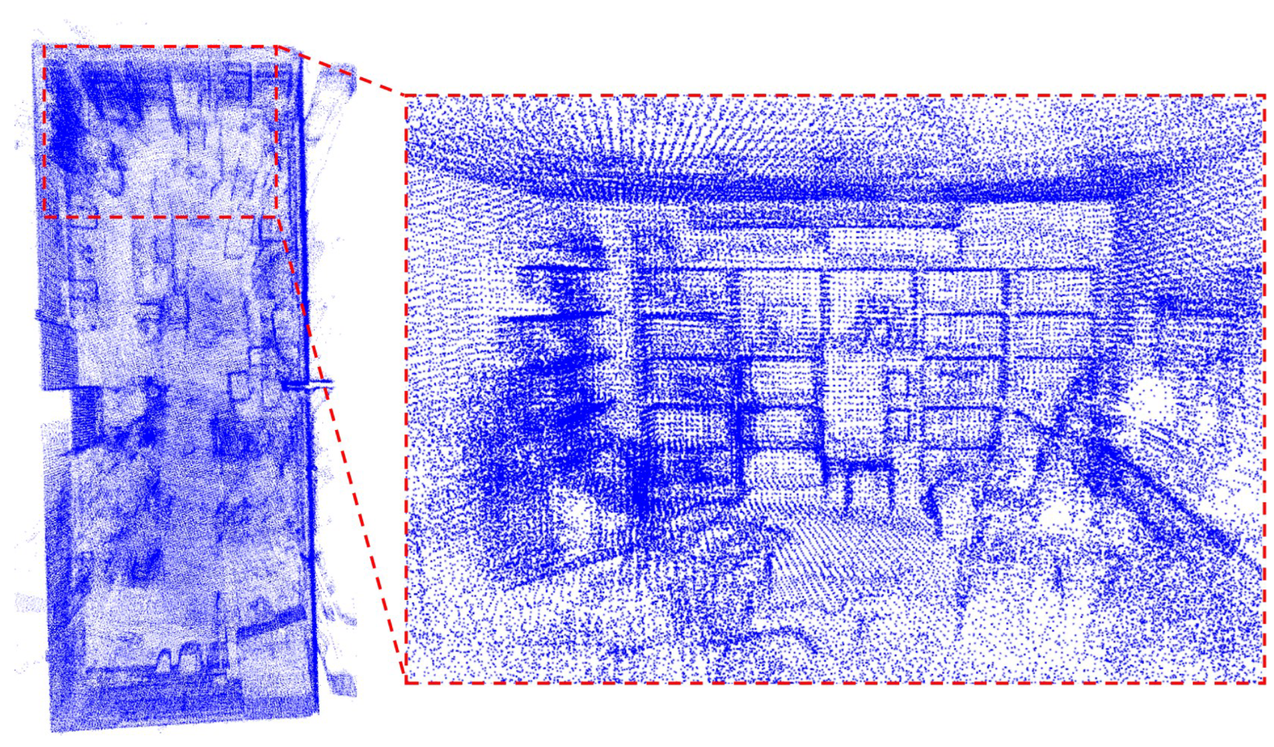
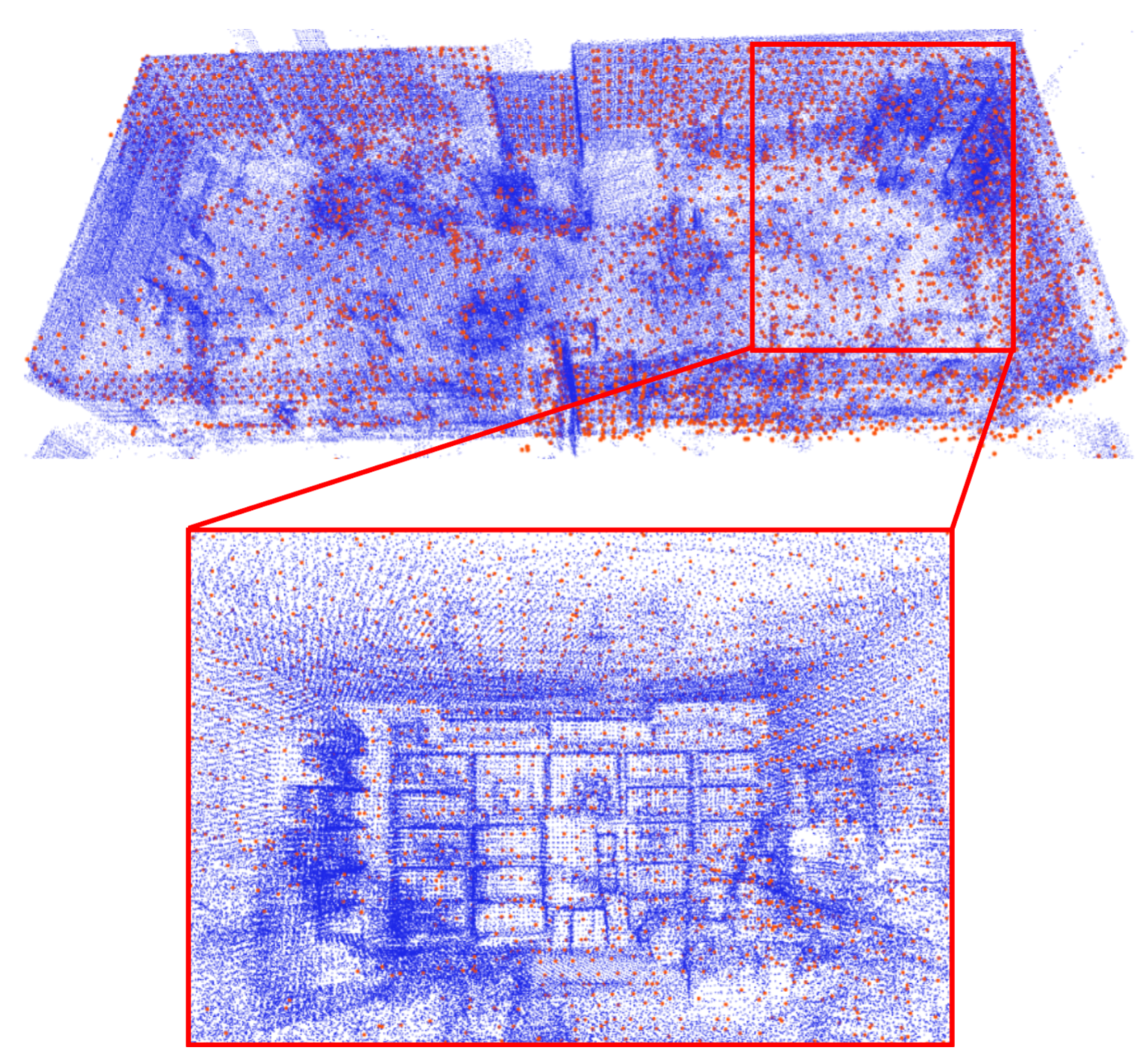
Inspired by the prior map generation methods in [24], where a survey-grade 3D imaging laser scanner Leica BLK360 is unitized to obtain static point clouds of the target environment, we employ a low-cost solid-state LiDAR Livox Avia and high-resolution spinning LiDAR to collect undistorted point clouds from environments. According to the Livox Avia datasheet, the range accuracy of the Avia sensor is 2 cm with a maximum detection range of 480 m. Due to the non-repetitive scanning pattern, the environment coverage of the point cloud within the FoV increases with time. Therefore, we integrate multiple frames when the platform is stationary to obtain more detailed undistorted environmental sampling. Each integrated point cloud contains more than 240,000 points. The Livox built-in IMU is used to detect the stationary state of the platform when the acceleration values are smaller than 0.01 along all axes. After gathering multiple undistorted point cloud submaps from the target environment, the next step is to match and merge all submaps into a global map by ICP. As the ICP process requires a good initial guess, we employ a high-resolution spinning LiDAR OS0 with a 360-degree horizontal FoV to provide the raw position by performing real-time SLAM algorithms. This process is outlined in Algorithm 1. A dense and high-definition ground truth map can be obtained by denoising the map generated by the algorithm described above to remove noise. Figure 1 shows the ground truth map of the sequence indoor08 generated based on Algorithm 1.
Let be the point cloud produced by the spinning LiDAR, be the point cloud generated by solid-state LiDAR, and be the IMU data from built-in IMU. Our previous work has shown high-resolution spinning LiDAR has the most robust performance in diverse environments. Therefore, LeGo-LOAM [15] is performed with a high-resolution spinning LiDAR (OS0-128) and outputs the estimated pose for each submap.
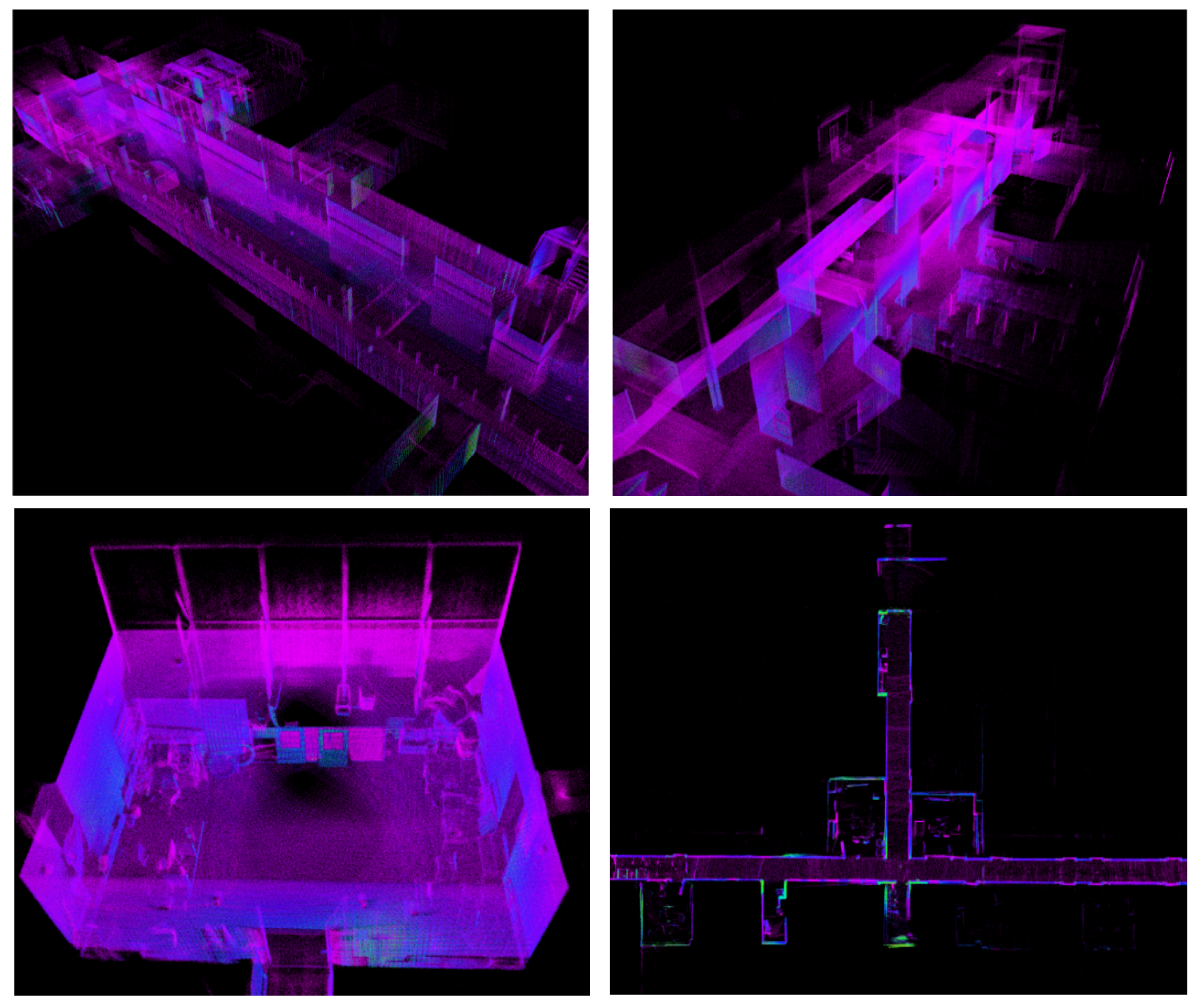
The cached data store the submaps and the related poses. Let be the point cloud and related pose in . The submap will be first transformed to map coordinate as based on the estimated pose ; then, generalized iterative closest point (GICP) methods are employed on to minimize the Euclidean distance between the closest points against point cloud iteratively; will be transformed by the transformation matrix generated from GICP process, and then merged to the map . The result map is treated as the ground truth map. Figure 4 provides a visual display of several ground truth maps, which have been acquired through the aforementioned procedural steps.
| Algorithm 1:SLAM-assisted ICP-based prior map generation for ground truth data |
 |
After the ground truth map is generated, we employ the normal NDT method in [25] to match the real-time point cloud data from the spinning LiDAR against the HR map as Figure 5 shows to obtain the platform position in the ground truth map. The matching result from the NDT localizer is treated as the ground truth.
4. SLAM Benchmark
In this study, we evaluated popular 3D LiDAR SLAM algorithms in multiple data sequences of various scenarios, including indoor, outdoor, and forest environments. The indoor data were collected from the office, corridor, and halls of ICT-City, Turku, and Finland. The forest data were gathered at a forest in (60°2814.3N, 22°1954.8E), Turku, Finland. Conversely, the road dataset was assembled from data collected at an open-air skating park, also situated in Turku, Finland. Further specifications pertaining to the dataset are comprehensively elaborated in Table 2.
4.1. Ground Truth Evaluation
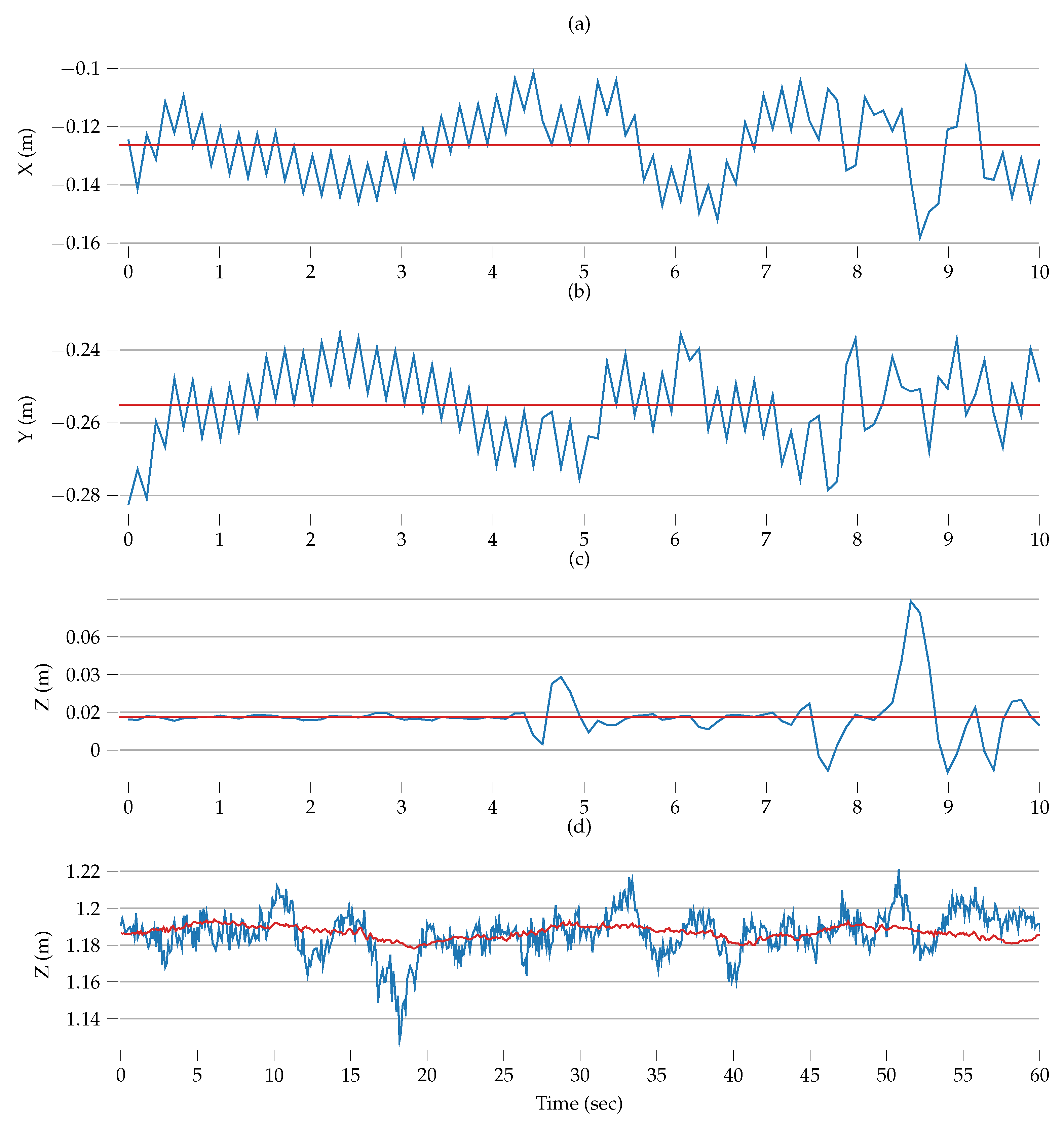
The evaluation of the accuracy of the proposed ground truth prior map method was challenging for some scenes in the dataset, as both the GNSS and MOCAP systems are not available in indoor environments, such as long corridors. To evaluate the generated ground truth, we adhered to the methodological approach delineated in the referenced study [24]. Figure 6a–c show the standard deviations of the ground truth generated by the proposed method during the first 10 seconds when the device was stationary from sequence Indoors09. The standard deviations along the X, Y, and Z axes are 2.2 cm, 4.1 cm, and 2.5 cm, respectively, or about 4.8 cm overall. However, evaluating the localization performance when the device was in motion was more difficult. To better understand the order of magnitude of the accuracy, we compared the NDT-based ground truth Z values with the MOCAP-based ground truth Z values in the sequence Indoor06 environment. The results in Figure 6d show that the maximum difference does not exceed 5 cm.
4.2. LiDAR Odometry Benchmarking
Different types of SLAM algorithms were selected and tested in our experiment. LiDAR-only algorithms LeGo-LOAM (LEGO) (https://github.com/RobustFieldAutonomyLab/LeGO-LOAM, accessed on 27 June 2023) and Livox-Mapping (LVXM) (https://github.com/Livox-SDK/livox_mapping, accessed on 27 June 2023) were applied on data from the VLP-16 and Horizon separately. Tightly coupled iterated extended Kalman filter-based methods, FAST-LIO (FLIO) (https://github.com/hku-mars/FAST_LIO, accessed on 27 June 2023) [18], were applied on both spinning LiDAR and solid-state LiDAR with built-in IMUs. A tightly coupled LiDAR inertial SLAM system based on sliding window optimization, LiLi-OM (https://github.com/KIT-ISAS/lili-om, accessed on 27 June 2023) [6], was tested with OS1 and Horizon. Furthermore, a tightly coupled method featuring sliding window optimization developed for Horizon LiDAR, LIO-LIVOX (LIOL) (https://github.com/Livox-SDK/LIO-Livox, accessed on 27 June 2023), was also tested on Horizon LiDAR data. When IMU was required, we used Avia’s IMU for Velodyne LiDAR results.
We provide a quantitative analysis of the odometry error based on the ground truth in Table 3. To compare the trajectories in the same coordinate, we treated the coordinate of OS0 as a reference coordinate and transformed all the trajectories generated by the selected SLAM methods to the reference coordinate. The absolute pose error (APE) [26] was employed as the core evaluation metric. We calculated the error of each trajectory with the open-source EVO toolset (https://github.com/MichaelGrupp/evo.git, accessed on 27 June 2023).
From the result, we can conclude that FAST_LIO with high-resolution spinning LiDAR OS0 and OS1 had the most robust performance that can complete all the trajectories on different sequences with promising accuracy. Especially for sequence Indoor09 showcasing a long corridor, all the other methods failed, and Fast_LIO with high-resolution LiDAR survived.
Solid-state LiDAR-based SLAM systems such as LIOL_Hori performed as well or even better in outdoor environments than rotating LiDARs with appropriate algorithms but performed significantly more poorly in indoor environments. For the open road sequences Road03, all the SLAM methods performed well, and the trajectories were completed without major disruptions. For the indoor sequence Indoor06, the Avia-based and Horizon-based FLIO were able to reconstruct the sensor trajectory, but significant drift accumulated. In all these sequences, all the methods applied to spinning LiDARs performed satisfactorily. This result can be expected as they have a full view of the environment, which has a clear geometry. For the sequence Indoor10 showcasing a long corridor, almost all the methods could reconstruct the complete trajectory again. The best performance came from OS0-FLIO and OS1-FLIO with correct alignment between the first and last positions. We hypothesize that this occurred because OS0 has more channels than OS1, leading to lower accumulated cumulative angular drift.
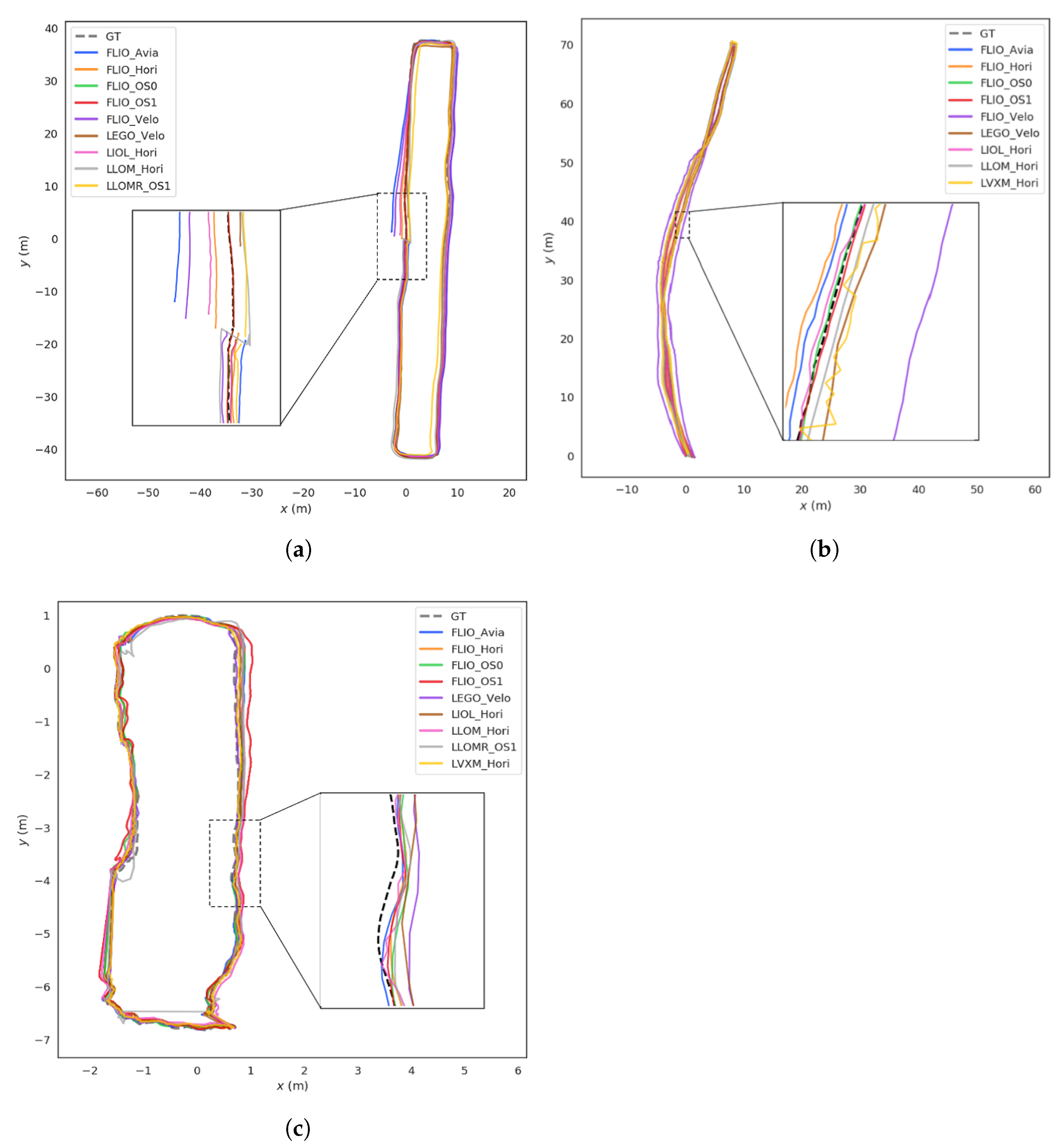
In addition to the quantitative trajectory analysis, we visualize trajectories generated by selected methods in three representative environments in Figure 7. Within this illustration, Figure 7a signifies the trajectory within an indoor setting, Figure 7b depicts the trajectory within an open road environment, and Figure 7c demonstrates the trajectory within a forest environment. Full reconstructed paths are available in the dataset repository.
4.3. Runtime Evaluation
We conducted this experiment on four different platforms. The first platform (1) was a Lenovo Legion Y7000P with 16 GB RAM, a 6-core Intel i5-9300H (2.40 GHz), and an Nvidia GTX 1660Ti (1536 CUDA cores, 6 GB VRAM). The second (2) platform was the Jetson Xavier AGX, a popular computing platform for mobile robots, which has an 8-core ARMv8.2 64-bit CPU (2.25 GHz), 16 GB RAM, and 512-core Volta GPU. From its 7 power modes, we chose MAX and 30 W (6-core only) modes. The third (3) platform was the Nvidia Xavier NX which is a common embedded computing platform with a 6-core ARM v8.2 64-bit CPU, 8 GB RAM, and 384-core Volta GPU with 48 Tensor cores. We chose the 15 W power mode (all 6 cores) for the NX. The fourth (4) platform was the UP Xtreme board featuring an 8-core Intel i7-8665UE (1.70 GHz) and 16 GB RAM.
These platforms all run ROS Melodic on Ubuntu 18.04. The CPU and memory utilization was measured with a ROS resource monitor tool (https://github.com/alspitz/cpu_monitor, accessed on 27 June 2023). Additionally, for minimizing the difference in the operating environment, we unified the dependencies used in each SLAM system into the same version, and each hyperparameter in the SLAM system was configured with the default values. The results are shown in Table 4.
The memory utilization of each selected SLAM approach among the two processor architectures platforms was roughly equivalent. However, the CPU utilization of the same SLAM algorithm running on Intel processors was generally higher than the other algorithms, and also the highest publishing frequency was obtained. LeGO_LOAM had the lowest CPU utilization, but its accuracy was toward the low end (see Table 4) and had a very low pose publishing frequency. Fast-LIO performed well, especially on embedded computing platforms, with good accuracy, low resource utilization, and high pose publishing frequency. In contrast, LIO_LIVOX had the highest CPU utilization due to the computational complexity of the frame-to-model registration method applied to estimate the pose.
A final takeaway is in the generalization of the studied methods. Many state-of-the-art methods are only applicable to a single LiDAR modality. In addition, those that have higher flexibility (e.g., FLIO) still lack the ability to support a point cloud resulting from the fusion of both types of LiDARs.
4.4. Mapping Quality Evaluation
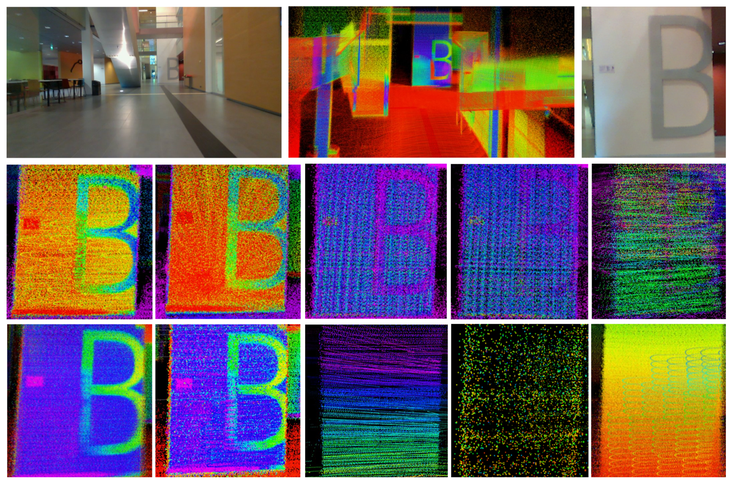
We qualitatively compare the mapping result generated from different LiDARs in indoor environments as shown in Figure 8.
From Figure 8, we can observe that the LIOL method applied to solid-state LiDAR presents the most detailed and clear map. It is worth noting that these maps have been generated with the default configuration of the methods and without changing parameters, such as the map update frequency. This result matches the quantitative results obtained with the same sensors and algorithms in the forest environment.
As shown in Figure 8, the Horizon-based LIOL has the best mapping ability, but if the environment (such as sequences indoors 06–09) is complex, LIOL will fail to map due to drift. In addition, OS0- and OS1-based FLIO also have good mapping ability, thanks to the wide FoV and excellent resolution of OS0 and OS1. Compared to OS0 and OS1, Velodyne has poorer mapping ability due to its larger resolution, and it has almost failed to reconstruct the letter B sign in Figure 8. LVMX, LLOM, and LLOMR focus on calculating the mobile platform’s pose estimation rather than point cloud mapping ability, so the point cloud maps they reconstructed are relatively poor.
5. Conclusions
In this paper, we provide LiDAR datasets covering the characteristics of various environments (indoor, outdoor, forest) and systematically evaluate five open-source SLAM algorithms in terms of LiDAR odometry and power consumption. The experiments have covered nine sequences across four computing platforms. Including the Nvidia Jetson Xavier platform provides further references for the application of various SLAM algorithms on computationally resource-constrained devices, such as drones. Overall, we found that in both indoor and outdoor environments, the spinning LiDAR-based FLIO exhibited good performance with low power consumption, which we believe is due to the ability of the spinning LiDAR to obtain a full view of the environment. However, in the forest environment, the LIOL algorithm based on solid-state LiDAR has the best accuracy and mapping quality performance, although it has the highest power consumption due to sliding window optimization.
Finally, we aim to further extend our dataset to provide more refined and difficult sequences and open source them in the future. In this paper, our benchmark tests only focus on SLAM algorithms based on spinning LiDAR and solid-state LiDAR. In the future, we will add benchmark tests based on cameras and even SLAM algorithms based on multiple sensor fusions.
Author Contributions
Conceptualization: Q.L. and J.P.Q.; methodology, H.S., Q.L. and J.P.Q.; software H.S. and Q.L.; data collection: H.S.; data processing and analysis: H.S.; writing: H.S., Q.L., J.P.Q., X.Y. and T.W.; visualization: H.S., Q.L., and X.Y.; supervision: J.P.Q., Z.Z. and T.W. All authors have read and agreed to the published version of the manuscript.
Funding
This research work is supported by the Academy of Finland’s AeroPolis project (Grant No. 348480).
Data Availability Statement
The data that support the work are available at the https://github.com/TIERS/tiers-lidars-dataset-enhanced (accessed on 27 June 2023).
Conflicts of Interest
The authors declare no conflict of interest.
References
- Li, Q.; Queralta, J.P.; Gia, T.N.; Zou, Z.; Westerlund, T. Multi-sensor fusion for navigation and mapping in autonomous vehicles: Accurate localization in urban environments. Unmanned Syst. 2020, 8, 229–237. [Google Scholar] [CrossRef]
- Varney, N.; Asari, V.K.; Graehling, Q. DALES: A large-scale aerial LiDAR data set for semantic segmentation. In Proceedings of the IEEE/CVF Conference on Computer Vision and Pattern Recognition Workshops, Seattle, WA, USA, 13–19 June 2020; pp. 186–187. [Google Scholar]
- Yang, J.; Kang, Z.; Cheng, S.; Yang, Z.; Akwensi, P.H. An individual tree segmentation method based on watershed algorithm and three-dimensional spatial distribution analysis from airborne LiDAR point clouds. IEEE J. Sel. Top. Appl. Earth Obs. Remote. Sens. 2020, 13, 1055–1067. [Google Scholar] [CrossRef]
- Van Nam, D.; Gon-Woo, K. Solid-state LiDAR based-SLAM: A concise review and application. In Proceedings of the 2021 IEEE International Conference on Big Data and Smart Computing (BigComp), Jeju Island, Republic of Korea, 17–20 January 2021; IEEE: Piscataway, NJ, USA, 2021; pp. 302–305. [Google Scholar]
- Qingqing, L.; Xianjia, Y.; Queralta, J.P.; Westerlund, T. Adaptive lidar scan frame integration: Tracking known mavs in 3d point clouds. In Proceedings of the 2021 20th International Conference on Advanced Robotics (ICAR), Ljubljana, Slovenia, 6–10 December 2021; IEEE: Piscataway, NJ, USA, 2021; pp. 1079–1086. [Google Scholar]
- Li, K.; Li, M.; Hanebeck, U.D. Towards high-performance solid-state-lidar-inertial odometry and mapping. IEEE Robot. Autom. Lett. 2021, 6, 5167–5174. [Google Scholar] [CrossRef]
- Queralta, J.P.; Qingqing, L.; Schiano, F.; Westerlund, T. VIO-UWB-based collaborative localization and dense scene reconstruction within heterogeneous multi-robot systems. In Proceedings of the 2022 International Conference on Advanced Robotics and Mechatronics (ICARM), IEEE, Guilin, Guangxi, China, 3–5 July 2022; pp. 87–94. [Google Scholar]
- Lin, J.; Zhang, F. Loam livox: A fast, robust, high-precision LiDAR odometry and mapping package for LiDARs of small FoV. In Proceedings of the 2020 IEEE International Conference on Robotics and Automation (ICRA), Paris, France, 31 May–31 August 2020; pp. 3126–3131. [Google Scholar]
- Li, Q.; Yu, X.; Queralta, J.P.; Westerlund, T. Multi-Modal Lidar Dataset for Benchmarking General-Purpose Localization and Mapping Algorithms. In Proceedings of the 2022 IEEE/RSJ International Conference on Intelligent Robots and Systems (IROS), Kyoto, Japan, 23–27 October 2022; pp. 3837–3844. [Google Scholar]
- Cadena, C.; Carlone, L.; Carrillo, H.; Latif, Y.; Scaramuzza, D.; Neira, J.; Reid, I.; Leonard, J.J. Past, present, and future of simultaneous localization and mapping: Toward the robust-perception age. IEEE Trans. Robot. 2016, 32, 1309–1332. [Google Scholar] [CrossRef] [Green Version]
- Rozenberszki, D.; Majdik, A.L. LOL: Lidar-only odometry and localization in 3D point cloud maps. In Proceedings of the 2020 IEEE International Conference on Robotics and Automation (ICRA), Paris, France, 31 May–31 August 2020; pp. 4379–4385. [Google Scholar]
- Zhen, W.; Zeng, S.; Soberer, S. Robust localization and localizability estimation with a rotating laser scanner. In Proceedings of the 2017 IEEE International Conference on Robotics and Automation (ICRA), Singapore, 29 May–3 June 2017; pp. 6240–6245. [Google Scholar]
- Ye, H.; Chen, Y.; Liu, M. Tightly coupled 3d lidar inertial odometry and mapping. In Proceedings of the 2019 International Conference on Robotics and Automation (ICRA), Montreal, QC, Canada, 20–24 May 2019; pp. 3144–3150. [Google Scholar]
- Zhang, J.; Singh, S. LOAM: Lidar Odometry and Mapping in Real-time. Robot. Sci. Syst. 2014, 2, 1–9. [Google Scholar]
- Shan, T.; Englot, B. Lego-loam: Lightweight and ground-optimized lidar odometry and mapping on variable terrain. In Proceedings of the 2018 IEEE/RSJ International Conference on Intelligent Robots and Systems (IROS), Madrid, Spain, 1–5 October 2018; pp. 4758–4765. [Google Scholar]
- Li, Q.; Nevalainen, P.; Peña Queralta, J.; Heikkonen, J.; Westerlund, T. Localization in Unstructured Environments: Towards Autonomous Robots in Forests with Delaunay Triangulation. Remote Sens. 2020, 12, 1870. [Google Scholar] [CrossRef]
- Nevalainen, P.; Movahedi, P.; Queralta, J.P.; Westerlund, T.; Heikkonen, J. Long-Term Autonomy in Forest Environment Using Self-Corrective SLAM. In New Developments and Environmental Applications of Drones; Springer: Cham, Switzerland, 2022; pp. 83–107. [Google Scholar]
- Xu, W.; Zhang, F. Fast-lio: A fast, robust lidar-inertial odometry package by tightly-coupled iterated kalman filter. IEEE Robot. Autom. Lett. 2021, 6, 3317–3324. [Google Scholar] [CrossRef]
- Xu, W.; Cai, Y.; He, D.; Lin, J.; Zhang, F. Fast-lio2: Fast direct lidar-inertial odometry. IEEE Trans. Robot. 2022, 38, 2053–2073. [Google Scholar] [CrossRef]
- Lin, J.; Zhang, F. R3LIVE: A Robust, Real-time, RGB-colored, LiDAR-Inertial-Visual tightly-coupled state Estimation and mapping package. In Proceedings of the 2022 International Conference on Robotics and Automation (ICRA), Philadelphia, PA, USA, 23–27 May 2022; pp. 10672–10678. [Google Scholar]
- Nguyen, T.M.; Cao, M.; Yuan, S.; Lyu, Y.; Nguyen, T.H.; Xie, L. Viral-fusion: A visual-inertial-ranging-lidar sensor fusion approach. IEEE Trans. Robot. 2021, 38, 958–977. [Google Scholar] [CrossRef]
- Geiger, A.; Lenz, P.; Stiller, C.; Urtasun, R. Vision meets robotics: The kitti dataset. Int. J. Robot. Res. 2013, 32, 1231–1237. [Google Scholar] [CrossRef] [Green Version]
- Lixia, M.; Benigni, A.; Flammini, A.; Muscas, C.; Ponci, F.; Monti, A. A software-only PTP synchronization for power system state estimation with PMUs. IEEE Trans. Instrum. Meas. 2012, 61, 1476–1485. [Google Scholar] [CrossRef]
- Ramezani, M.; Wang, Y.; Camurri, M.; Wisth, D.; Mattamala, M.; Fallon, M. The newer college dataset: Handheld lidar, inertial and vision with ground truth. In Proceedings of the 2020 IEEE/RSJ International Conference on Intelligent Robots and Systems (IROS), Las Vegas, NV, USA, 24 October 2020–24 January 2021; pp. 4353–4360. [Google Scholar]
- Biber, P.; Straßer, W. The normal distributions transform: A new approach to laser scan matching. In Proceedings of the 2003 IEEE/RSJ International Conference on Intelligent Robots and Systems (IROS 2003) (Cat. No. 03CH37453), Las Vegas, NV, USA, 27–31 October 2003; Volume 3, pp. 2743–2748. [Google Scholar]
- Sturm, J.; Engelhard, N.; Endres, F.; Burgard, W.; Cremers, D. A benchmark for the evaluation of RGB-D SLAM systems. In Proceedings of the 2012 IEEE/RSJ International Conference on Intelligent Robots and Systems(IROS), Vilamoura-Algarve, Portugal, 7–12 October 2012; pp. 573–580. [Google Scholar]
Figure 1.
Ground truth map for one of the indoor sequences generated based on the proposed approach (SLAM-assisted ICP-based prior map). This enables benchmarking of LiDAR odometry and mapping algorithms in larger environments where a motion capture system or similar is not available, with significantly higher accuracy (<2 cm) than GNSS/RTK solutions.

Figure 2.
Front view of the multi-modal data acquisition system. Next to each sensor, we show the individual coordinate frames.
Figure 2.
Front view of the multi-modal data acquisition system. Next to each sensor, we show the individual coordinate frames.

Figure 3.
Top view of point cloud data generated for the calibration process with multiple LiDARs. The red and green point clouds represent data obtained from the Livox Horizon and Avia, respectively. The purple, yellow, blue, and black clouds are from the VLP-16, OS1, OS0, and L515 sensors, respectively.

Figure 4.
Samples of map data form different dataset sequences. From left to right and top to bottom, we display maps generated from sequences indoors09, indoors11, indoors06, and indoors10, respectively.
Figure 4.
Samples of map data form different dataset sequences. From left to right and top to bottom, we display maps generated from sequences indoors09, indoors11, indoors06, and indoors10, respectively.

Figure 5.
NDT localization with ground truth map. External view and internal view when the current laser scan (orange) is aligned with the ground truth map (blue).
Figure 5.
NDT localization with ground truth map. External view and internal view when the current laser scan (orange) is aligned with the ground truth map (blue).

Figure 6.
(a–c) Ground truth position values for the first 10 s of the dataset when the device was stationary. Red lines show the mean values over this period of time. (d) Comparison of NDT-based ground truth z-values (blue) to MOCAP-based z-values (red) over the course of 60 s of the dataset while the device was in motion.

Figure 7.
Demos of trajectories generated by multiple 3D LiDAR SLAM based on data from indoor, road, and wild environments. (a) Trajectory comparison of sequence Indoor10; (b) trajectory comparison of sequence Road03; (c) trajectory comparison of sequence Forest01.
Figure 7.
Demos of trajectories generated by multiple 3D LiDAR SLAM based on data from indoor, road, and wild environments. (a) Trajectory comparison of sequence Indoor10; (b) trajectory comparison of sequence Road03; (c) trajectory comparison of sequence Forest01.

Figure 8.
Qualitative comparison of the mapping quality. The first row from left to right shows RGB full-view image, full-view Horizon-based LIOL, and close-view RGB image. The second row from left to right shows OS0, OS1, Velodyne, Avia, and Horizon-based FLIO. The bottom row from left to right shows the Horizon-based LIOL, Horizon, OS1-based LLOM and LLOMR, Velodyne’s LeGo-LOAM maps, and Horizon-based LVXM, respectively.


Table 1.
Sensor specification for the presented dataset. Angular resolution is configurable in OS1-64 (varying the vertical FoV). Livox LiDARs have a non-repetitive scan pattern that delivers higher angular resolution with longer integration times. For LiDARs, range is based on manufacturer information, with values corresponding to 80% Lambertian reflectivity and 100 klx sunlight, except for the L515 LiDAR camera.
| Sensor | IMU | Type | Channels | FoV | Resolution | Range | Freq. | Points (pts/s) |
|---|---|---|---|---|---|---|---|---|
| VLP-16 | N/A | spinning | 16 | 360° × 30° | V: 2.0°, H: 0.4° | 100 m | 10 Hz | 300,000 |
| OS1-64 | ICM-20948 | spinning | 64 | 360° × 45° | V: 0.7°, H: 0.18° | 120 m | 10 Hz | 1,310,720 |
| OS0-128 | ICM-20948 | spinning | 128 | 360° × 90° | V: 0.7°, H: 0.18° | 50 m | 10 Hz | 2,621,440 |
| Horizon | BS-BMI088 | solid state | N/A | 81.7° × 25.1° | N/A | 260 m | 10 Hz | 240,000 |
| Avia | BS-BMI088 | solid state | N/A | 70.4° × 77.2° | N/A | 450 m | 10 Hz | 240,000 |
| L515 | BS-BMI085 | LiDAR camera | N/A | 70° × 43° (°) | N/A | 9 m | 30 Hz | - |
| T265 | BS-BMI055 | fisheye cameras | N/A | 163 ± 5° | N/A | N/A | 30 Hz | - |
Table 2.
List of data sequences in our extended dataset. The table includes the sequences introduced in our previous work [9], together with new sequences showcasing new ground truth data sources. The five LiDARs indicated (5x LiDARs) and cameras are listed in Table 1.
| Sequence | Description | Ground Truth | Sensor Setup | |
|---|---|---|---|---|
| Forest01-03 | Previous dataset [9] | MOCAP/SLAM |  | 5x LiDARs |
| Indoor01-05 | Previous dataset [9] | MOCAP/SLAM | L515 | |
| Road01-02 | Previous dataset [9] | SLAM | Optitrack | |
| Indoor06 | Lab space (easy) | MOCAP |  | |
| Indoor07 | Lab space (hard) | MOCAP | 5x LiDARs | |
| Indoor08 | Classroom space | SLAM+ICP | L515 | |
| Indoor09 | Corridor (short) | SLAM+ICP | T265 | |
| Indoor10 | Corridor (long) | SLAM+ICP | Optitrack | |
| Indoor11 | Hall (large) | SLAM+ICP | GNSS | |
| Road03 | Open road | GNSS RTK | ||
Table 3.
Absolute position error (APE) () in cm of the selected methods (N/A when odometry estimations diverge). Best results in bold.
Table 3.
Absolute position error (APE) () in cm of the selected methods (N/A when odometry estimations diverge). Best results in bold.
| Sequence | FLIO_OS0 | FLIO_OS1 | FLIO_Velo | FLIO_Avia | FLIO_Hori | LLOM_Hori | LLOMR_OS1 | LIOL_Hori | LVXM_Hori | LEGO_Velo |
|---|---|---|---|---|---|---|---|---|---|---|
| Indoor06 | 0.015/0.006 | 0.032/0.011 | N/A | 0.205/0.093 | 0.895/0.447 | N/A | 0.882/0.326 | N/A | N/A | 0.312/0.048 |
| Indoor07 | 0.022/0.007 | 0.025/0.013 | 0.072/0.031 | N/A | N/A | N/A | N/A | N/A | N/A | 0.301/0.081 |
| Indoor08 | 0.048/0.030 | 0.042/0.018 | 0.093/0.043 | N/A | N/A | N/A | N/A | N/A | N/A | 0.361/0.100 |
| Indoor09 | 0.188/0.099 | N/A | 0.472/0.220 | N/A | N/A | N/A | N/A | N/A | N/A | N/A |
| Indoor10 | 0.197/0.072 | 0.189/0.074 | 0.698/0.474 | 0.968/0.685 | 0.322/0.172 | 1.122/0.404 | 1.713/0.300 | 0.641/0.469 | N/A | 0.930/0.901 |
| Indoor11 | 0.584/0.080 | 0.105/0.041 | 0.911/0.565 | 0.196/0.098 | 0.854/0.916 | 0.1.097/0.0.45 | 1.509/0.379 | N/A | N/A | N/A |
| Road03 | 0.123/0.032 | 0.095/0.037 | 1.001/0.512 | 0.211/0.033 | 0.351/0.043 | 0.603/0.195 | N/A | 0.103/0.058 | 0.706/0.396 | 0.2464/0.063 |
| Forest01 | 0.138/0.054 | 0.146/0.087 | N/A | 0.142/0.074 | 0.125/0.062 | 0.116/0.053 | 0.218/0.110 | 0.054/0.033 | 0.083/0.041 | 0.064/0.032 |
| Forest02 | 0.127/0.065 | 0.121/0.069 | N/A | 0.211/0.077 | 0.348/0.077 | 0.612/0.198 | N/A | 0.125/0.073 | 0.727/0.414 | 0.275/0.077 |
Table 4.
Average run-time resource (CPU/RAM) utilization and performance (pose calculation speed) comparison of selected SLAM methods across multiple platforms. The data are played at 15 times the real speed for the pose publishing frequency. CPU utilization of 100% equals one full processor core.
Table 4.
Average run-time resource (CPU/RAM) utilization and performance (pose calculation speed) comparison of selected SLAM methods across multiple platforms. The data are played at 15 times the real speed for the pose publishing frequency. CPU utilization of 100% equals one full processor core.
| (CPU Utilization (%), RAM Utilization (MB), Pose Publication Rate (Hz)) | |||||
|---|---|---|---|---|---|
| Intel PC | AGX MAX | AGX 30 W | UP Xtreme | NX 15 W | |
| FLIO_OS0 | (79.4, 384.5, 74.0) | (40.9, 385.3, 13.6) | (55.1, 398.8, 13.2) | (90.9, 401.8, 47.3) | (53.7, 371.1, 14.3) |
| FLIO_OS1 | (73.7, 437.4, 67.5) | (54.5, 397.5, 21.2) | (73.9, 409.2, 15.4) | (125.9, 416.2, 58.0) | (73.3, 360.4, 14.2) |
| FLIO_Velo | (69.9, 385.2, 98.6) | (44.4, 369.7, 29.1) | (58.3, 367.6, 21.4) | (110.5, 380.5, 89.6) | (57, 331.5, 19.5) |
| FLIO_Avia | (65.0, 423.8, 98.3) | (40.8, 391.5, 32.3) | (47.4, 413.4, 24.5) | (113.2, 401.2, 90.7) | (51.2, 344.8, 21.9) |
| FLIO_Hori | (65.7, 423.8, 103.7) | (37.6, 408.4, 34.7) | (50.5, 387.9, 26.8) | (109.7, 422.8, 91.0) | (47.5, 370.7, 23.4) |
| LLOM_Hori | (126.2, 461.6, 14.5) | (128.5, 545.4, 9.1) | (168.5, 658.5, 1.5) | (130.1, 461.1, 12.8) | (N/A) |
| LLOMR_OS1 | (112.3, 281.5, 25.8) | (70.8, 282.3, 9.6) | (107.1, 272.2, 6.5) | (109.0, 253.5, 13.6) | (N/A) |
| LIOL_Hori | (186.1, 508.7, 19.1) | (247.2, 590.3, 9.6) | (188.1, 846.0, 4.1) | (298.2, 571.8, 14.0) | (239.0, 750.5, 4.54) |
| LVXM_Hori | (135.4, 713.7, 14.7) | (162.3, 619.0, 10.5) | (185.86, 555.81, 5.0) | (189.6, 610.4, 7.9) | (198.0, 456.7, 5.5) |
| LEGO_Velo | (28.7, 455.4, 9.8) | (42.4, 227.8, 7.0) | (62.8, 233.4, 3.5) | (39.7, 256.6, 9.1) | (36.9, 331.4, 3.7) |
Disclaimer/Publisher’s Note: The statements, opinions and data contained in all publications are solely those of the individual author(s) and contributor(s) and not of MDPI and/or the editor(s). MDPI and/or the editor(s) disclaim responsibility for any injury to people or property resulting from any ideas, methods, instructions or products referred to in the content. |
© 2023 by the authors. Licensee MDPI, Basel, Switzerland. This article is an open access article distributed under the terms and conditions of the Creative Commons Attribution (CC BY) license (https://creativecommons.org/licenses/by/4.0/).
Share and Cite
MDPI and ACS Style
Sier, H.; Li, Q.; Yu, X.; Peña Queralta, J.; Zou, Z.; Westerlund, T. A Benchmark for Multi-Modal LiDAR SLAM with Ground Truth in GNSS-Denied Environments. Remote Sens. 2023, 15, 3314. https://doi.org/10.3390/rs15133314
AMA Style
Sier H, Li Q, Yu X, Peña Queralta J, Zou Z, Westerlund T. A Benchmark for Multi-Modal LiDAR SLAM with Ground Truth in GNSS-Denied Environments. Remote Sensing. 2023; 15(13):3314. https://doi.org/10.3390/rs15133314
Chicago/Turabian StyleSier, Ha, Qingqing Li, Xianjia Yu, Jorge Peña Queralta, Zhuo Zou, and Tomi Westerlund. 2023. "A Benchmark for Multi-Modal LiDAR SLAM with Ground Truth in GNSS-Denied Environments" Remote Sensing 15, no. 13: 3314. https://doi.org/10.3390/rs15133314
Note that from the first issue of 2016, this journal uses article numbers instead of page numbers. See further details here.