
Uncertainty of CYGNSS-Derived Heat Flux Variations at Diurnal to Seasonal Time Scales over the Tropical Oceans


1
Key Laboratory of Marine Science and Numerical Modeling, First Institute of Oceanography, Ministry of Natural Resources, Qingdao 266061, China
2
Laboratory for Regional Oceanography and Numerical Modeling, Pilot National Laboratory for Marine Science and Technology, Qingdao 266237, China
3
Shandong Key Laboratory of Marine Science and Numerical Modeling, Qingdao 266061, China
*
Author to whom correspondence should be addressed.
Remote Sens. 2023, 15(12), 3161; https://doi.org/10.3390/rs15123161
Submission received: 25 April 2023
/
Revised: 13 June 2023
/
Accepted: 15 June 2023
/
Published: 17 June 2023
(This article belongs to the Special Issue Advanced Applications of Remote Sensing in Monitoring Marine Environment)
Abstract
:Air–sea heat flux is one of the most important factors that affects ocean circulation, weather, and climate. Satellite remote sensing could serve as an important supplement to the sparse in situ observations for heat flux estimations. In this study, we analyze the uncertainty of the turbulent heat fluxes derived from wind speed measured by the Cyclone Global Navigation Satellite System (CYGNSS) over the global tropical oceans at different time scales. In terms of spatial distribution, there is large uncertainty (approximately 50 to 85 W·m−2 in the RMSE) near the equator in the western Pacific Ocean, the Arabian Sea, the Bay of Bengal, and near the Gulf of Guinea. The turbulent heat fluxes are in agreement with the buoys in representing the intraseasonal and seasonal variability, but more specific regional validations are needed for revealing the synoptic and sub-synoptic phenomena and the diurnal cycle. The uncertainty of the CYGNSS wind speed contributes approximately 50–57% to the uncertainty of the estimation of turbulent heat fluxes at the frequency band with a typical period of 3–7 days. In addition, the input sea surface temperature, rather than the wind speed, results in differences in the estimation of the monthly mean turbulent heat fluxes in the tropical Atlantic Ocean based on the COARE 3.5 algorithm. In conclusion, although the CYGNSS-derived turbulent heat fluxes are basically in good agreement with the in situ observations, our analysis highlights the importance of considering the limitations of these datasets, particularly in high wind speed conditions and for higher-frequency variations, including at synoptic, sub-synoptic, and diurnal time scales.
1. Introduction
The air–sea heat flux is fundamentally important for understanding the interaction and energy exchange between the atmosphere and ocean. By definition, the air–sea heat flux consists of the solar shortwave and infrared longwave radiative fluxes and the surface latent and sensible heat fluxes [1,2,3]. The surface latent heat flux (LHF) represents the amount of heat extracted from the ocean during seawater evaporation, while the surface sensible heat flux (SHF) represents the amount of heat extracted from the ocean due to the temperature difference between the air and sea. The LHF and SHF are also referred to as turbulent heat fluxes because both of them are induced by turbulent mixing.
The LHF and SHF are typically estimated by a “bulk flux algorithm” based on the observed state variables of the ocean and atmosphere, i.e., the wind speed, relative humidity (RH), air temperature and density, sea level pressure (SLP), and sea surface temperature (SST) [4,5,6,7]. Of these state variables, they can be directly measured by in situ platforms, such as ships, flux towers, moored buoys, drifting buoys, wave gliders, and unmanned vessels, or retrieved by satellite sensors, such as microwave scatterometer and radiometer, doppler lidar, Synthetic Aperture Radar (SAR), Global Navigation Satellite System-Reflectometry (GNSS-R) sensors, altimeter, infrared radiometer, etc. [7].
However, turbulent heat fluxes obtained from in situ observations are limited in spatial and temporal coverage. In comparison, satellite-derived turbulent heat fluxes could provide more information to benefit broader coverage and real-time transmission of the data. However, their accuracy should be validated against in situ observations to ensure their reliability. Bentamy et al. [8] assessed the accuracy of the LHF and SHF derived from microwave radiometry, scatterometry, and infrared radiometry, suggesting that they matched well with those from moored buoys, as shown in scatter diagrams. Other LHF and SHF products based on satellite observations combined with numerical models (e.g., IFREMER, GSSTF, NCEP-NCAR, OAFLUX, HOAPS, J-OFURO2, J-OFURO3, MERRA, and GSFC) have also been validated in good agreement with in situ observations in scatter diagrams [8,9,10,11,12,13,14,15,16,17,18]. In terms of temporal and spatial variations, however, these products are less accurate under either high or low wind speed conditions. In addition, the limitations of remote sensing instruments, i.e., infrequent coverage and signals attenuated by precipitation and cloud, also result in deficiencies of LHF and SHF products [8,19,20]. Nevertheless, satellite remote sensing has an advantage in its operational application due to its high efficiency and low cost, and thus, importantly contributes to monitoring the variables of the atmosphere and ocean [21,22].
The Cyclone Global Navigation Satellite System (CYGNSS) satellite constellation, launched by NASA at the end of 2016, consists of eight microsatellites, each of which can receive four reflections simultaneously within one second, allowing for a total of thirty-two wind speed measurements per second globally, with a spatial resolution of 25 km on the specular point [23]. Therefore, the CYGNSS platform has the advantage of monitoring tropical cyclones by allowing for the unprecedented detection of the surface wind speed in the inner core of tropical cyclones, with refined spatial and temporal resolution. The wind speed products of the CYGNSS are continuously updated and developed, and have been used as important supplements to in situ observation data [24,25,26,27,28,29,30,31]. The CYGNSS provides improved estimations of the LHF and SHF over the tropical and subtropical oceans using its high temporal and spatial sampling of the sea surface wind speed [26,28]. Crespo et al. (2019) proposed an estimate of CYGNSS heat fluxes by employing the Coupled Ocean-Atmosphere Response Experiment (COARE) 3.5 algorithm based on the CYGNSS surface wind speed combined with the temperature and humidity from the MERRA-2 reanalysis data. They validated the CYGNSS heat fluxes by comparing them with buoy observations, showing overall consistency and root mean square errors (RMSEs) of around 40 W/m2 and 10 W/m2 for the LHF and SHF, respectively. Later, they released two versions of the CYGNSS heat flux products. CDR V1.0 and CDR V1.1 were evaluated, showing overall averaged RMSEs of 33.60 W/m2 and 6.77 W/m2 for the LHF and SHF, respectively, for CDR V1.1, slightly better than those for CDR V1.0 [28]. Previously, an assessment of CYGNSS heat fluxes also suggested that their uncertainties may be associated with the inputs from the MERRA-2 and different versions of wind speed products [26,28]. In summary, the existing studies have tended to assess the mean state of CYGNSS heat fluxes. The uncertainties of CYGNSS heat fluxes in representing the variations at different time scales, i.e., diurnal, sub-synoptic, synoptic, intraseasonal, and seasonal, however, have not been revealed. The contribution of input variables, i.e., the CYGNSS wind speed, as well as the MERRA-2 temperature and humidity, to the uncertainties of estimating heat fluxes at different time scales have not been quantitatively provided.
In this study, we try to reveal the uncertainties of CYGNSS heat fluxes at different time scales based on wavelet coherence analysis and to provide a quantitative estimation of contributions to the uncertainty based on the ensemble empirical mode decomposition (EEMD) method. The sensitivity of different input variables for the CYGNSS heat flux calculation and the uncertainties of CYGNSS heat fluxes in different ocean basins are also discussed.
2. Data and Methods
2.1. Turbulent Heat Flux Calculation
The COARE algorithm and bulk aerodynamic formulas are widely employed to calculate turbulent heat fluxes [3,7,32]. The conventional Monin–Obukhov similarity theory (MOST) was used to develop the COARE algorithm, which was based on the Liu–Katsaros–Businger methodology, and was later updated by Fairall et al. [33]. For wind speeds of 0–10 m/s and 10–20 m/s, COARE 3.0 achieves accuracies within 5% and 10%, respectively. The COARE algorithm exhibited the fewest problems, according to a study by Brunke et al. [34], which examined 12 bulk aerodynamic algorithms for computing turbulent heat fluxes. After four outfield experiments, COARE 3.5 enhanced the parameterization of the surface roughness and drag coefficients and offered greater accuracy for heat flux predictions at wind speeds up to 25 m/s [6]. Therefore, we employed the COARE 3.5 to calculate the LHF and SHF, based on the input variables of wind speed, air temperature and density, air specific humidity, and SST.
The bulk aerodynamic formulas for estimating LHF and SHF are as follows [4]:
where 𝜌𝑎 is the density of the atmosphere within the sea surface boundary layer; 𝑈, 𝑞𝑎, and 𝑇𝑎 are the wind speed, specific humidity, and air temperature at 10 m; 𝑞𝑠 is the air specific humidity at the sea surface and 𝑇𝑠 is the SST; 𝐿𝑣 is the latent heat of evaporation or condensation, 𝑐p is the specific heat at a constant pressure; and 𝐶DE and 𝐶DH are the latent and sensible heat exchange coefficients, which are parameterized in COARE 3.5 as a function of gust, surface roughness, and atmospheric stability [6].
LHF = 𝜌𝑎𝐿𝑣𝐶𝐷𝐸𝑈(𝑞𝑠 − 𝑞𝑎)
SHF = 𝜌𝑎𝑐𝑝𝐶𝐷𝐻𝑈(𝑇𝑠 − 𝑇𝑎)
2.2. CYGNSS Wind Product
The improved secondary Climate Data Record (CDR) v1.1 wind speed product of CYGNSS (as opposed to CDR v1.0) is principally used in this paper. The data utilized are accessible at the NASA website (https://podaac-tools.jpl.nasa.gov/drive/files/allData/cygnss, accessed on 30 September 2022) and cover the period from 1 August 2018 (the earliest data available in CDR v1.1) to 31 December 2021. The accuracy of the heat fluxes obtained in this work utilizing the COARE 3.5 algorithm, CYGNSS wind speeds, and other inputs from MERRA-2 was also verified using a corresponding CYGNSS CDR v1.1 heat flux product. On the aforementioned website, the heat flux product is also accessible. The CYGNSS wind speed data used in this study have been quality-controlled by filtering out the low-quality samples according to their sample flags.
2.3. MERRA-2 Reanalysis Data
NASA developed the Second Modern Retrospective Analysis for Research and Applications (MERRA-2) atmospheric reanalysis dataset using an improved Goddard Earth Observing System Model (GEOS-5) data assimilation system [35]. The 10-m eastward and northward wind, surface skin temperature and humidity, air temperature, humidity and density, and sea level pressure from the MERRA-2 reanalysis were employed for this research [36,37]. The specific data collections and variables used in this study are presented in Table 1. These data can be obtained from the website of the NASA Office of Global Modeling and Assimilation (https://gmao.gsfc.nasa.gov/reanalysis/MERRA-2/data_access/, accessed on 30 September 2022).
2.4. GTMBA Buoy Array Data
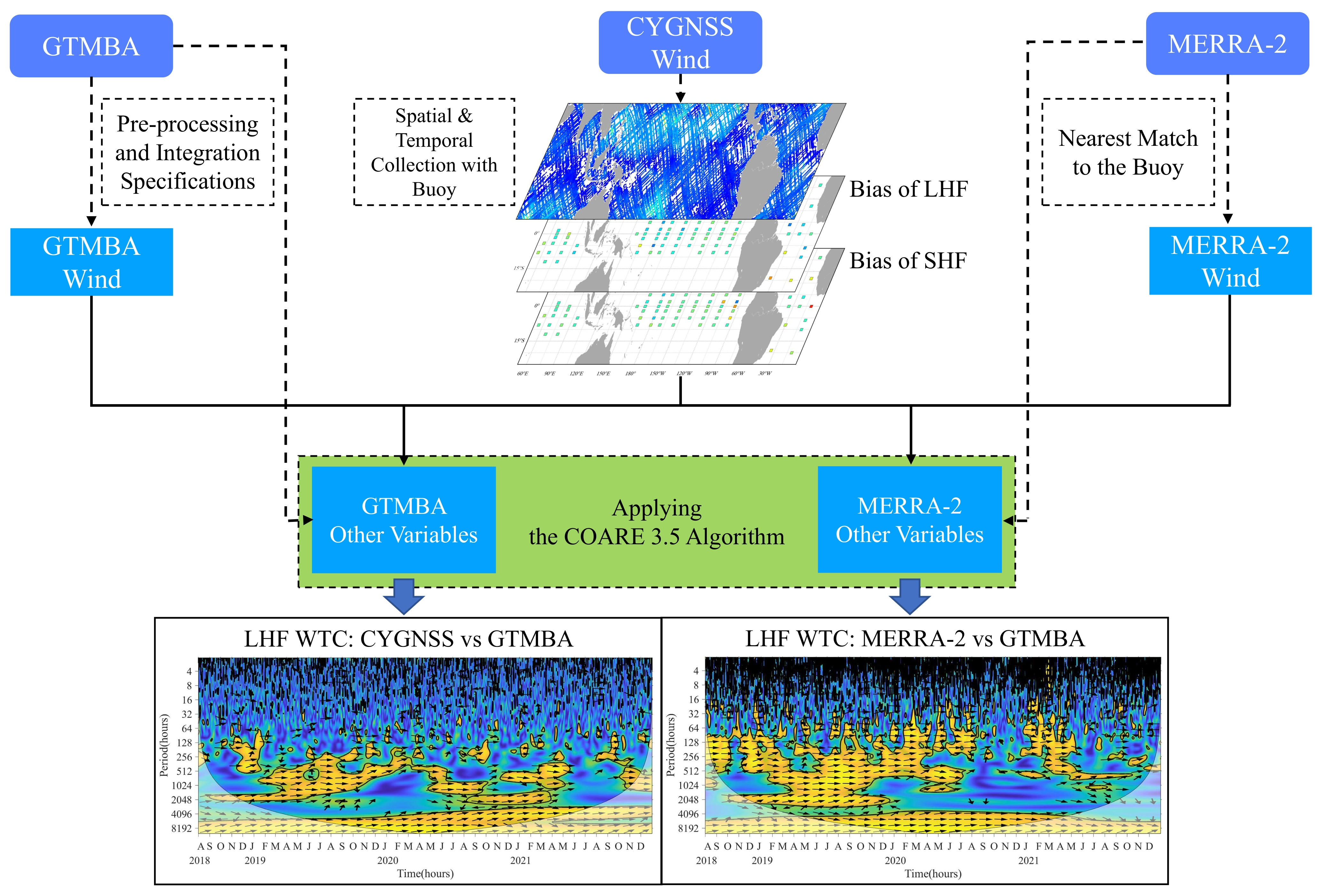
An international project called the Global Tropical Moored Buoy Array (GTMBA) aims to gather information for use in climate research and forecasting. Components of the global array include the Tropical Atmosphere Ocean/Triangle Trans-Ocean Buoy Network (TAO/TRITON) in the Pacific, the Prediction and Research Moored Array in the Tropical Atlantic (PIRATA), and the Research Moored Array for African–Asian–Australian Monsoon Analysis and Prediction (RAMA) in the Indian Ocean. For this study, we used all available related data from the GTMBA from 1 August 2018 to 31 December 2021, totaling 93 buoys.
Figure 1 displays the arrangement of the buoys that were used to collect data on the sea temperature, sea level pressure, wind speed at a 4 m height, and temperature and relative humidity at a 3 m altitude. In standard buoy measurements, the sea temperature is typically recorded at a depth ranging from 0.2 m to 1 m. In this study, we utilized these measurements as the sea surface temperature values, following the methodology employed in previous studies [6,33]. All data were preprocessed to an hourly resolution before being utilized for the formal analysis. Despite the fact that a large number of buoys had missing sea-level pressure measurements, our validation shows that adopting the MERRA-2 sea-level pressure hardly had an effect on the heat flux computation when the other input variables were held constant. Thus, the missing buoy sea-level pressure data were replaced with those of MERRA-2.
Equations (3) and (5) were used to obtain the saturation water vapor pressure (es) and air specific humidity at the sea surface (𝑞𝑠), and Equations (4) and (6) were used to translate the relative humidity (RH) into the air specific humidity at the buoy observation height (𝑞o).
where es is the saturation vapor pressure; e is the vapor pressure, and p is the SLP.
Equations (7)–(9) were used to obtain the 10 m wind speed (𝑈), 10 m air temperature (𝑇𝑎), and 10 m air specific humidity (𝑞a).
where Us is the velocity of the ocean surface current, set as 0; κ is the von Kármán constant, set as 0.4; To is the air temperature at the buoy observation height; zo, zoT, and zoq are the roughness length for the wind, air temperature, and humidity; φ and ϕ are the empirical functions describing the stability dependence of the shear profiles for the wind speed and temperature and humidity; L is the Monin–Obukhov length; and U*, T*, q* are the MOST scaling factors, determined iteratively by the COARE 3.5 bulk algorithm.
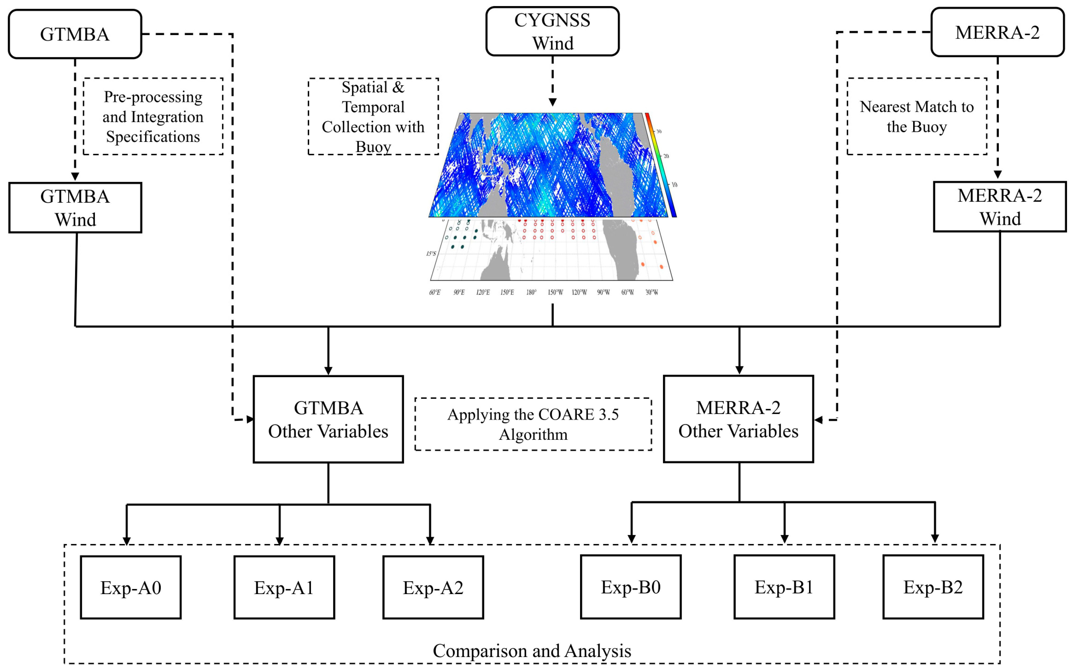
2.5. The Design of Sensitivity Experiments
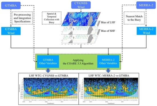
To evaluate the biases of the LHF and SHF associated with a 10 m wind speed (𝑈) versus the other input variables (i.e., 𝜌𝑎, 𝑞𝑠, 𝑞a, 𝑇𝑠, and 𝑇𝑎) derived from the CYGNSS and MERRA-2 reanalysis products, we designed two classes of sensitivity experiments with input variables from the CYGNSS, buoy, and MERRA-2 datasets for calculating the LHF and SHF using the COARE3.5 algorithm (Table 2). The biases of the outputted LHF and SHF between experiments A1 and A0 and between A2 and A0 are attributed to the difference in the 10 m wind speed of the CYGNSS and MERRA-2 products. The biases of the outputted LHF and SHF between experiments B0 and A0, B1 and A1, and B2 and A2 are attributed to the differences in the other input variables.
Figure 2 provides an illustration of the technical procedure. Prior to conducting the experiments, it was necessary to ensure consistent spatial and temporal alignment of each input variable, with the location of the buoys serving as a benchmark for matching with the other data sources. The CYGNSS observations were matched with the buoy stations with distance and time intervals of less than 50 km and 0.5 h, respectively. The MERRA-2 data were matched with the buoy station based on the nearest neighbor method. All variables were averaged into hourly time intervals. The statistical metrics and differences in the LHF and SHF derived from the sensitivity experiments at hourly, daily, and monthly time scales were then analyzed.
2.6. Major Evaluation Indicators
The statistical metrics of the root mean square error (RMSE), standard deviation (σ), mean bias (μ), and correlation coefficient (r) were employed to evaluate the biases of the LHF and SHF derived from different input variables and calculated as follows:
where x and y refer to the output variables of each group of experiments, and N is the sample number.
3. Results
3.1. Statistical Metrics of the Heat Fluxes Derived from Different Datasets
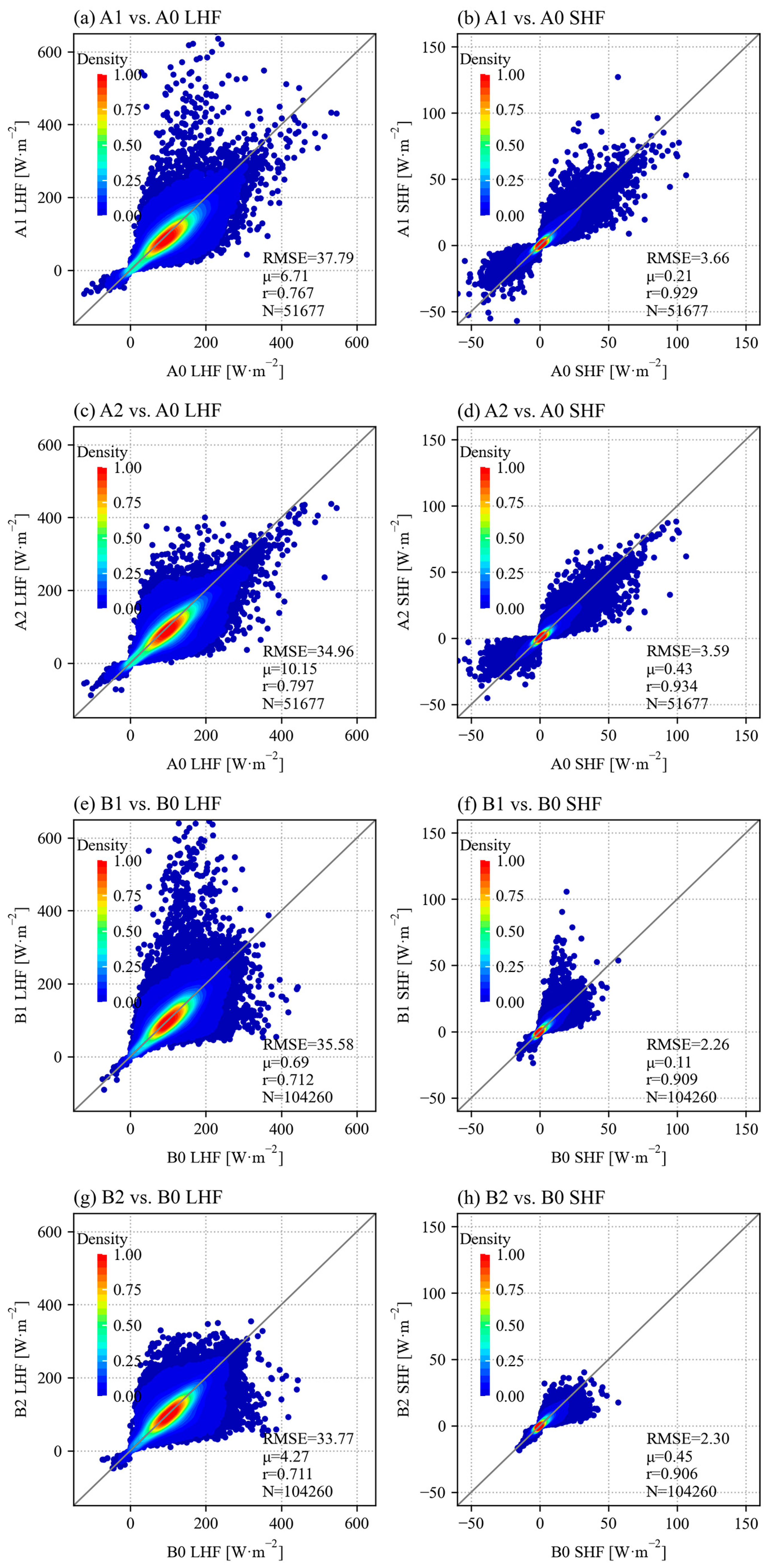
We compared the LHF and SHF estimates from A0 and from A1 and A2, and those from B0 and from B1 and B2. The corresponding statistical metrics are given in Figure 3. Each panel has the same time span from 1 August 2018 to 31 December 2021. It can be seen that the RMSEs of the A1- and A0-matched LHF and SHF were 37.79 W·m−2 and 3.66 W·m−2, respectively (Figure 3a,b). The RMSEs of the A2- and A0-matched LHF and SHF were 34.96 W·m−2 and 3.59 W·m−2, respectively (Figure 3c,d). We applied the same time–space matching criteria to both A1 and A2 with respect to A0, yielding an identical matched quantity of 51,677. This time–space selection was derived from the matching process between A1 and A0. The highest scatterplot density of the LHF occurred between 50 and 150 W·m−2, and that of the SHF occurred between −5 and 5 W·m−2. There were outliers in A1 when the LHF was larger than 400 W·m−2 (Figure 3a).
The RMSEs of the matched LHF and SHF for B1 and B0 were 35.58 W·m−2 and 2.26 W·m−2, respectively (Figure 3e,f), while the corresponding values for B2 and B0 were 33.77 W·m−2 and 2.3 W·m−2 (Figure 3g,h). As shown in Figure 3, the RMSEs of the LHF for B1 and B2 were reduced by only 5.8% and 3.4% compared to those of A1 and A2, respectively. However, the RMSEs of the SHF were reduced by 38% and 36%. Note that the sample number is the same for B1 and B2, based on the same explanation for A1 and A2. The outliers were still present in B1 when compared to A1, as displayed in Figure 3e. Additionally, the SHF values above 50 W·m−2 also exhibit outliers in Figure 3f.
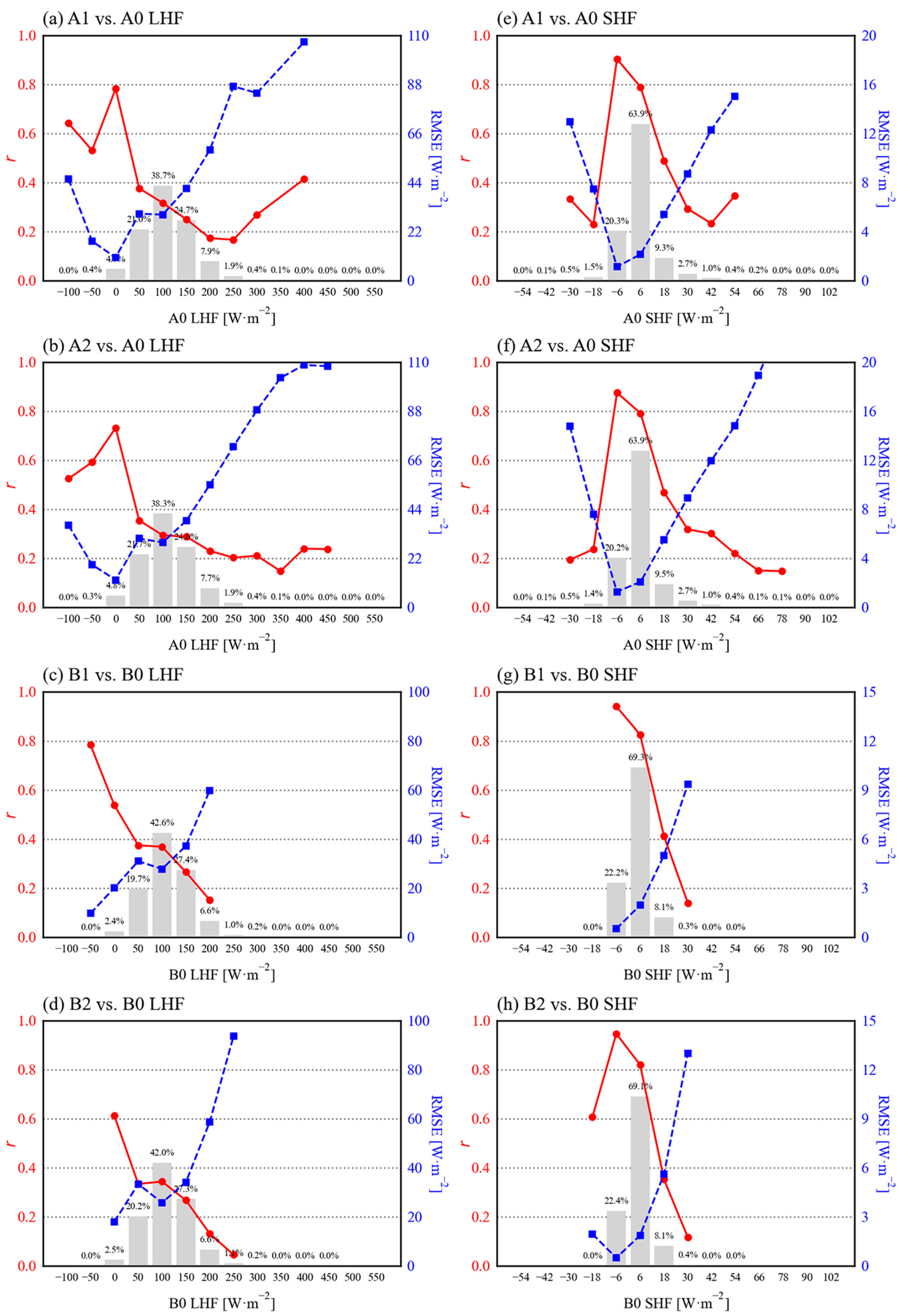
The LHFs derived from the different experiments generally fell in a range of approximately −25 to 300 W·m−2, and roughly 38~43% were within 75~125 W·m−2 (Figure 4a–d). The LHFs of A1 and A2 fit well with that of A0 at the range of −25 to 175 W·m−2, as evidenced by significant correlation coefficients greater than 0.28 and an RMSE smaller than 40 W·m−2 (25% of the mean value), respectively (Figure 4a,b). While the LHFs were greater than 225 W·m−2, they fit poorly with each other, with correlation coefficients smaller than 0.2 and an RMSE greater than 85 W·m−2 (35% of the mean value). The linear relationships of the LHFs for B1 and B2 with B0 were similar to those of A1 and A2 with A0, except that the LHFs of class B were generally smaller than 250 W·m−2 (Figure 4c,d). The SHFs derived from the different experiments generally fell in a range of approximately −24 to 36 W·m−2, and roughly 64~69% were within 0~12 W·m−2 (Figure 4e,f). The SHFs of A1 and A2 fit well with A0 with a range of −12 to 24 W·m−2, as evidenced by significant correlation coefficients greater than 0.48 and an RMSE smaller than 5.2 W·m−2 (25% of the mean value), respectively (Figure 4e,f). While the SHFs were smaller than −12 W·m−2 and greater than 24 W·m−2, they fit poorly with each other, with correlation coefficients smaller than 0.3 and an RMSE greater than 7.9 W·m−2 (30% of the mean value). The linear relationships for the SHFs of B1 and B2 with B0 were similar to those of A1 and A2 with A0, except that the SHFs of class B were generally smaller than 30 W·m−2 (Figure 4g,h).
3.2. Sensitivities of Different Input Wind Speed Datasets for the Heat Flux Calculation
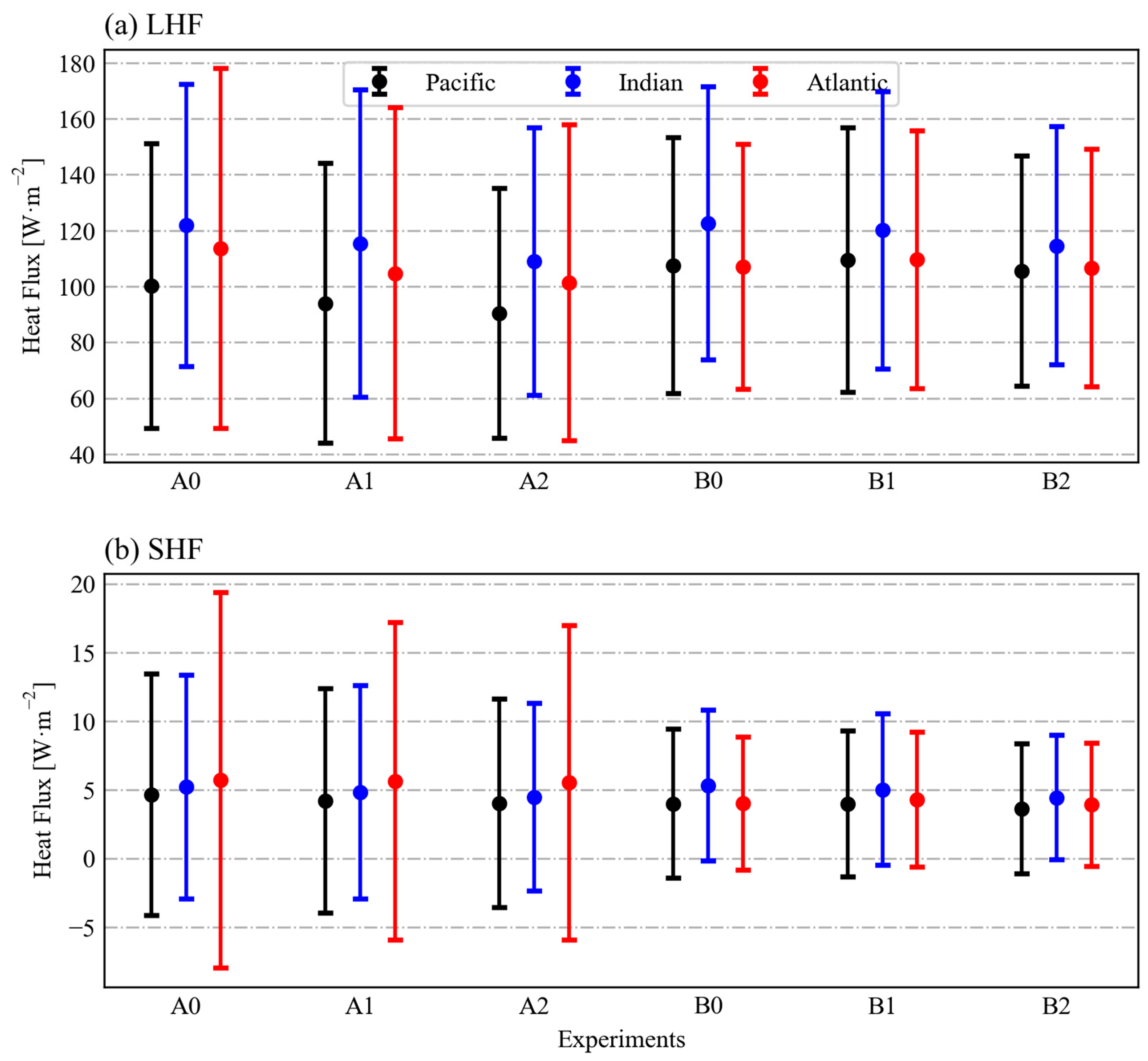
Figure 5 shows the area-averaged LHF and SHF over the period of 1 August 2018 to 31 December 2021 in the tropical Pacific, Indian, and Atlantic Oceans. There were significant differences in the LHF derived from different combinations of the input wind speed and state variables in the tropical oceans, with consistently higher estimates observed in the Indian Ocean. Among the experiments conducted in the Pacific Ocean, Indian Ocean, and Atlantic Ocean, experiment A2 had the smallest LHF, and experiments A0, B0, and B1 had the largest LHF. The experiments closest to A0 (buoy values) were B2, B0, and B1, respectively, in the same order for all three oceans. Based on the same other input variables from the buoys (A1 and A2), the LHFs estimated by the CYGNSS wind and MERRA-2 wind were lower than those of the buoy wind by about 6~9 W·m−2 and 10~13 W·m−2, respectively. The LHFs estimated by the other MERRA-2 inputs were greater than the LHFs estimated by the other buoy inputs for the Pacific, Indian, and Atlantic Oceans by around 15, 5, and 5 W·m−2, correspondingly, based on the identical wind input from CYGNSS (A1 and B1).
The SHFs lacked distinguishing characteristics, with only minor variations across the experiments and typically low heat flux levels. Based on the same other inputs from the buoys (A1 and A2), the SHFs estimated by the CYGNSS wind and MERRA-2 wind were lower than those of the buoy wind by about 0~2 W·m−2 and 1~3 W·m−2, respectively. It is noteworthy that in the estimation of the SHF for the Atlantic Ocean, the class B experiments commonly displayed lower values than the class A experiments.
3.3. Spatial Distribution of Mean Bias and RMSE in the Heat Fluxes
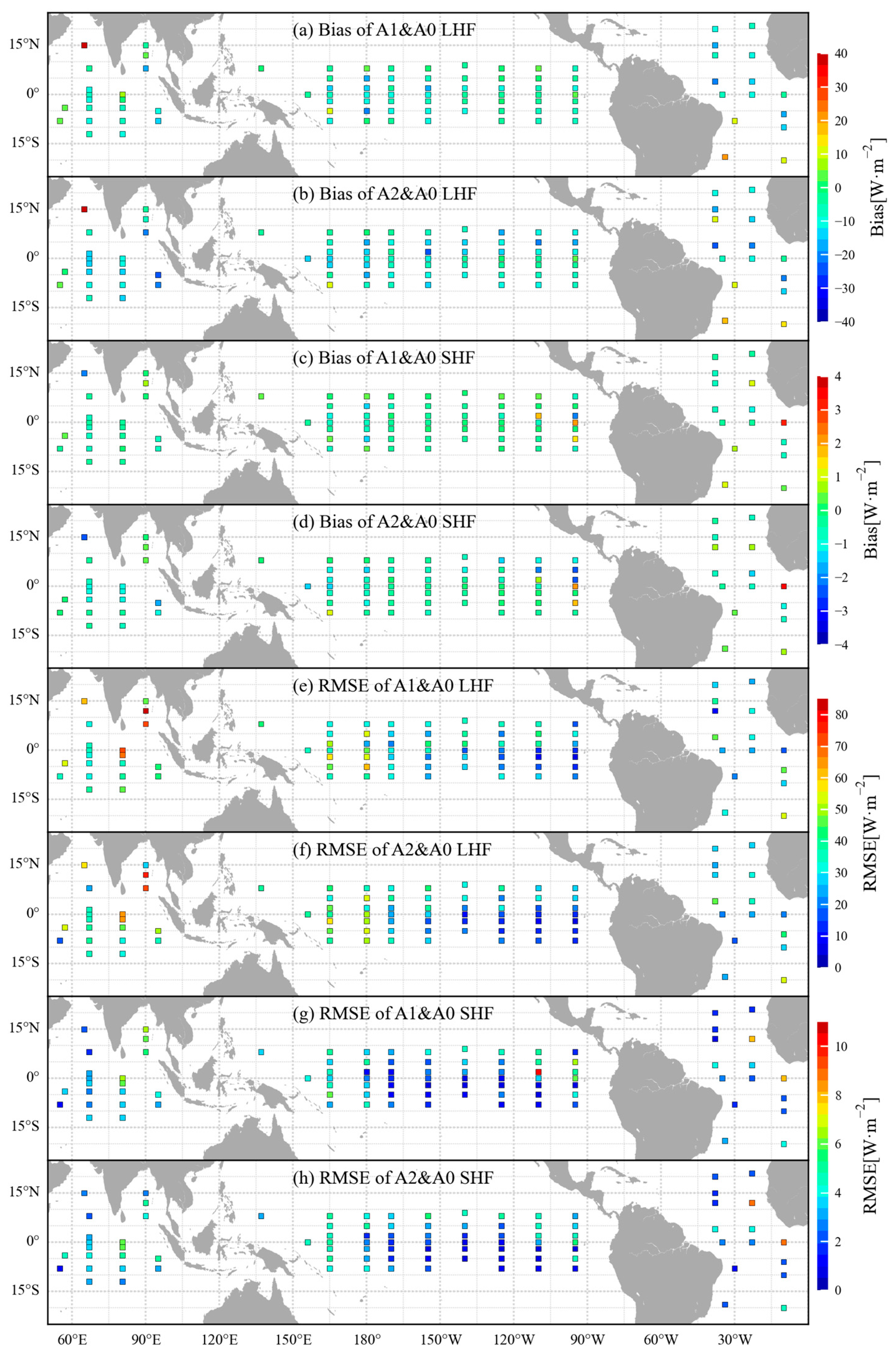
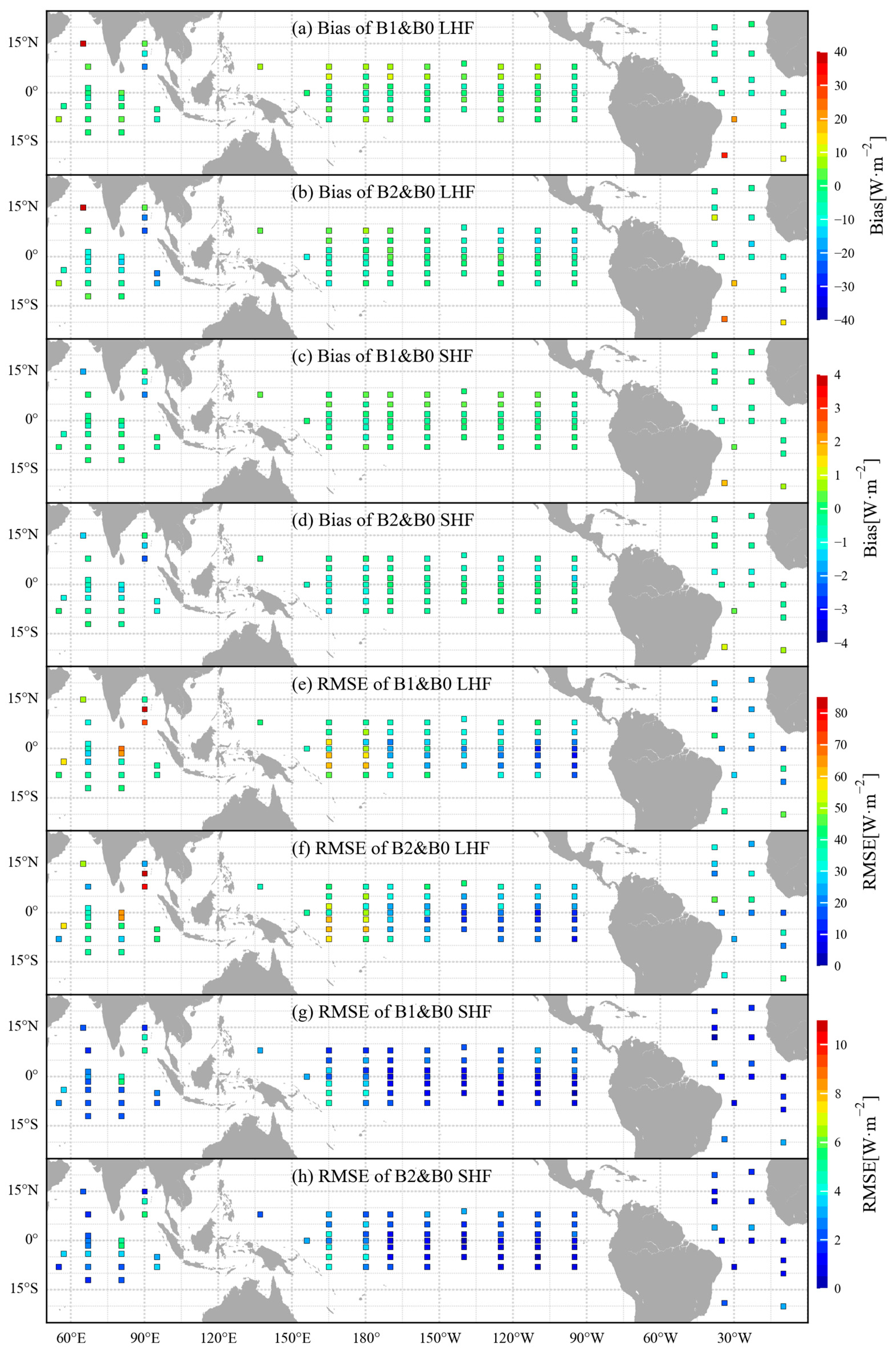
Figure 6 shows the spatial distribution of the biases and RMSEs of the LHF and SHF derived from experiments A1 and A2 with respect to A0 in the tropical oceans. The biases in the LHF were generally between −12 and 10 W·m−2, except for those in the Arabian Sea (65°E, 15°N) and the southwest Atlantic (34°W, 19°S), where the LHFs were overestimated by up to 40 and 28 W·m−2, respectively, and those in the southeastern tropical Indian Ocean (95°E, 5°S), the central equatorial Pacific Ocean (155°W, 0°N), and the off-equatorial north Atlantic Ocean (38°W, 4°N), where the LHFs were underestimated by approximately 20 W·m−2 (Figure 6a,b). The biases in the SHF were also larger in the Arabian Sea (65°E, 15°N), with underestimations of approximately −2 and −2.3 W·m−2 in experiments A1 and A2, respectively (Figure 6c,d). In addition, there were largely overestimated biases in the SHF in the equatorial eastern Pacific Ocean (95°W, 0°N) and the equatorial eastern Atlantic Ocean (10°W, 0°) (Figure 6c,d). In terms of the RMSE, those of the LHF were relatively large in the Indian Ocean, particularly in the Bay of Bengal, with a maximum value of approximately 85 W·m−2 at (90°E, 12°N) (Figure 6e). Large RMSEs were also observed in the Indo-Pacific warm pool near the equator, while the RMSEs were significantly smaller over the equatorial cold tongues of the Pacific and Atlantic Oceans (Figure 6e,f). The overall RMSEs of the SHF were small, with the largest RMSE occurring at the site (110°W, 2°N) in the eastern equator of the Pacific Ocean (Figure 6g), and two sites with large RMSEs existing on the eastern side of the tropical Atlantic Ocean (Figure 6g,h). The site (65°E, 15°N) with a large bias and RMSE in the Arabian Sea had only 11 matching sizes between A1 and A0, and 162 matching sizes between A2 and A0. With respect to the other sites, the matching size was relatively small, and the bias and RMSE of the site may have a lower reliable reference. The RMSEs of the LHF and SHF derived from the CYGNSS wind and MERRA-2 wind in the sites located in other areas (e.g., the Bay of Bengal, the Western Pacific Warm Pool, and the Gulf of Guinea) were greater than 50/4 W·m−2 and could reach a maximum value of 85/8.7 W·m−2, respectively.
In comparison to Figure 6, Figure A1 demonstrates a similar spatial distribution of bias and RMSE, including the distribution of larger biases and RMSEs. However, some differences exist, such as the absence of higher bias and RMSE values in the SHF of the Atlantic Ocean. Moreover, the maximum RMSE of the SHF at the eastern equatorial site (110°W, 2°N) in the Pacific Ocean, observed in Figure 6g, is absent from Figure A1g.
3.4. Wavelet Coherence Analysis of the Hourly Heat Fluxes
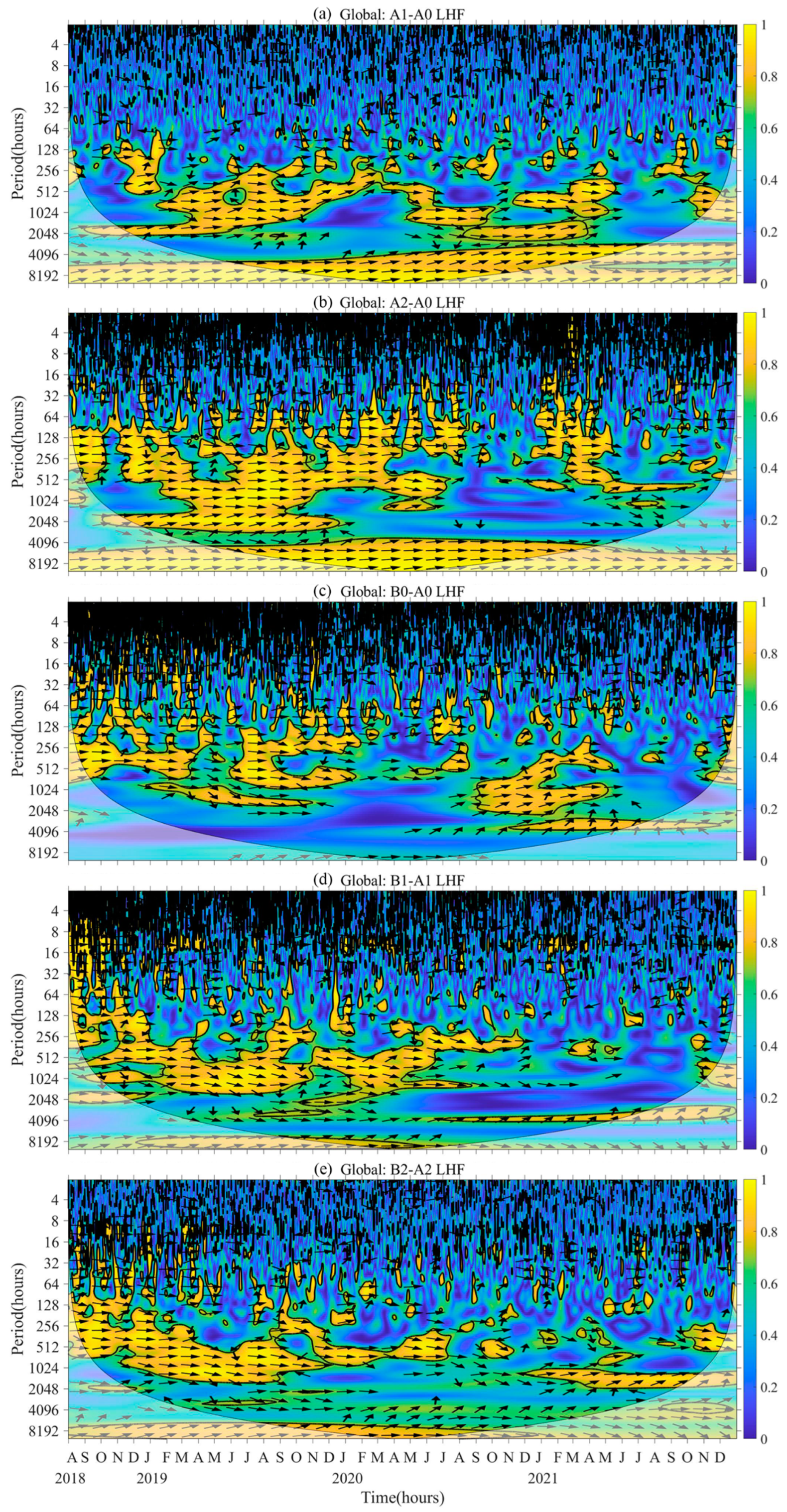
In this section, we analyze the consistency and dispersion of the LHFs and SHFs based on different wind speeds and other variables, i.e., the different outputs of the experiments in Table 2. Here, we employed wavelet coherence (WTC) to investigate the common spectral features of the LHFs and SHFs between these sequences (Figure 7). Wavelet coherence is a method used to find a localized correlation coefficient of two time series in a frequency space [38]. In the diagram, the rightward and leftward arrows indicate that the time series are in phase and out of phase, respectively, whereas the upward and downward arrows indicate the time series are in half-phase lag.
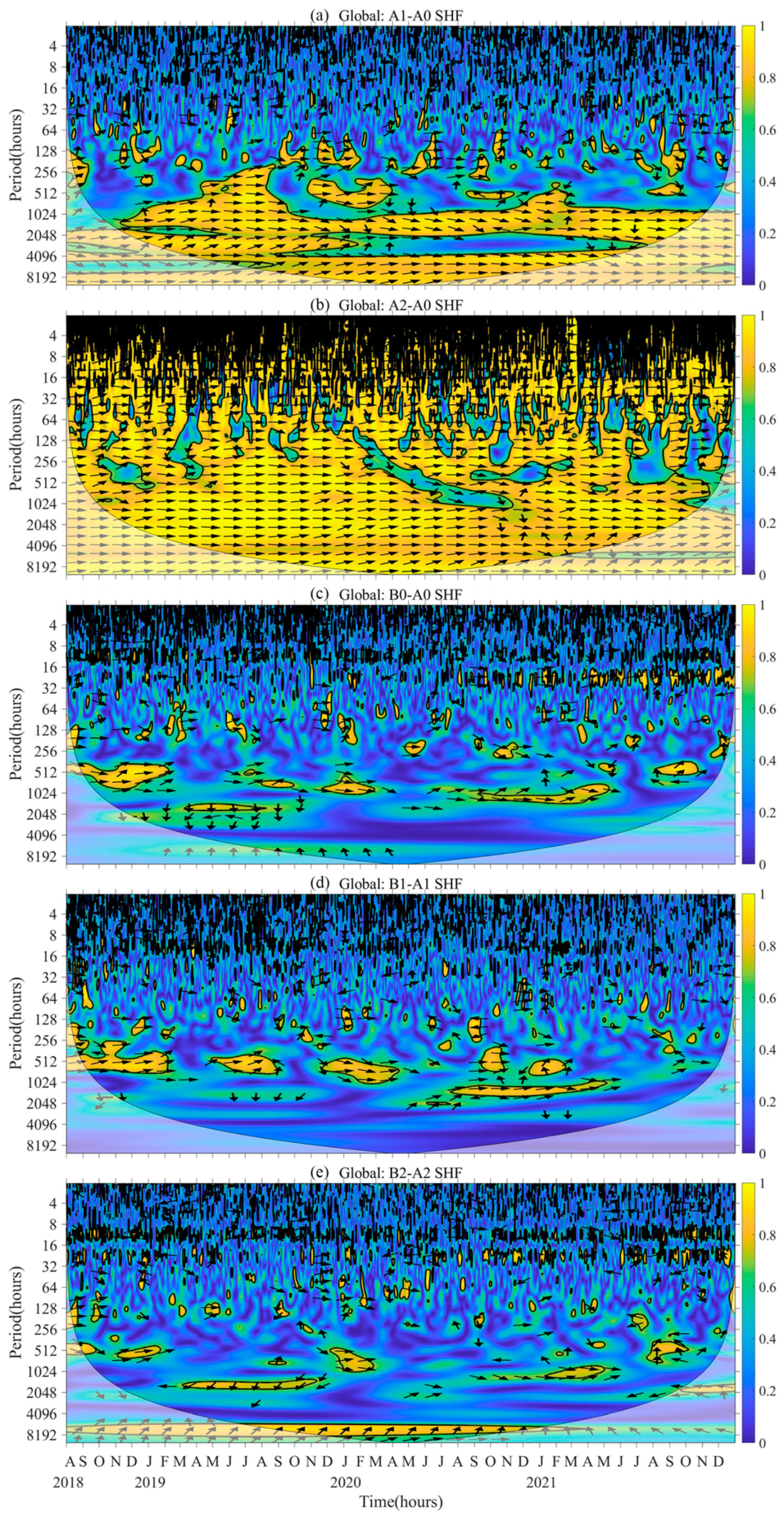
As shown in Figure 7, the LHFs derived from different input variables were generally simultaneous with each other at a low-frequency band with typical periods of approximately 5–90 days and greater than 6 months for experiments A1 and A2 with A0 (Figure 7a,b), and 10–90 days between experiment classes A and B (Figure 7c–e). On the contrary, the LHFs did not show significant coherence with each other at a high-frequency band with typical periods smaller than 5 days (including the diurnal cycle) throughout the observation period. These results suggest that the LHFs derived from the CYGNSS and MERRA-2 reanalysis are reliable for investigations and applications at the intraseasonal and seasonal time scales. However, for the synoptic, sub-synoptic, and diurnal time scales, the LHFs not only derived from the CYGNSS but also other input variables should be further validated before application. A similar WTC analysis was conducted for the SHFs (Figure 8). The results also suggest that the CYGNSS SHFs are reliable at the intraseasonal and seasonal time scales, but need further validation at the synoptic, sub-synoptic, and diurnal time scales.
3.5. Contributions of Wind Speed and Other Variables to Heat Fluxes Calculation
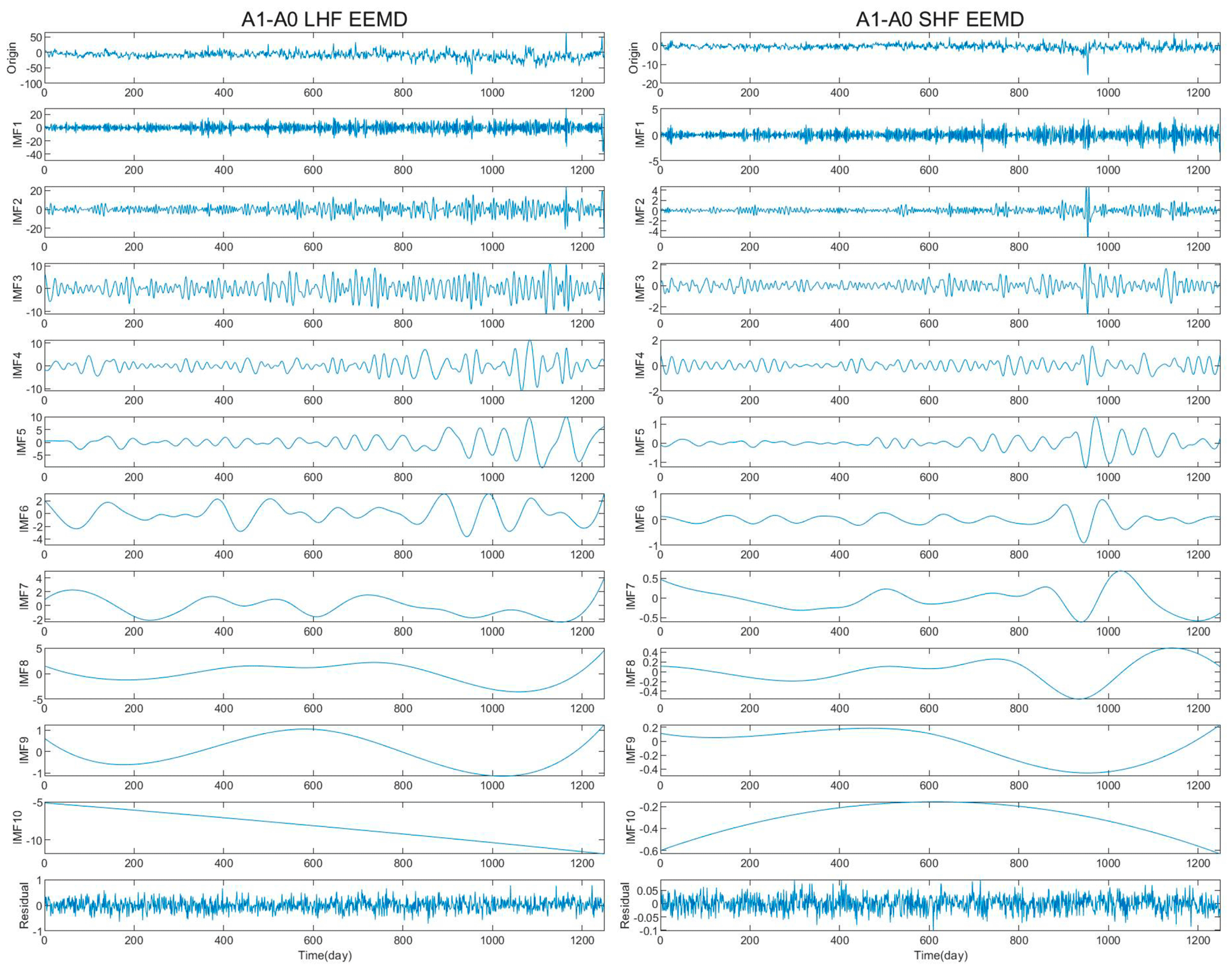
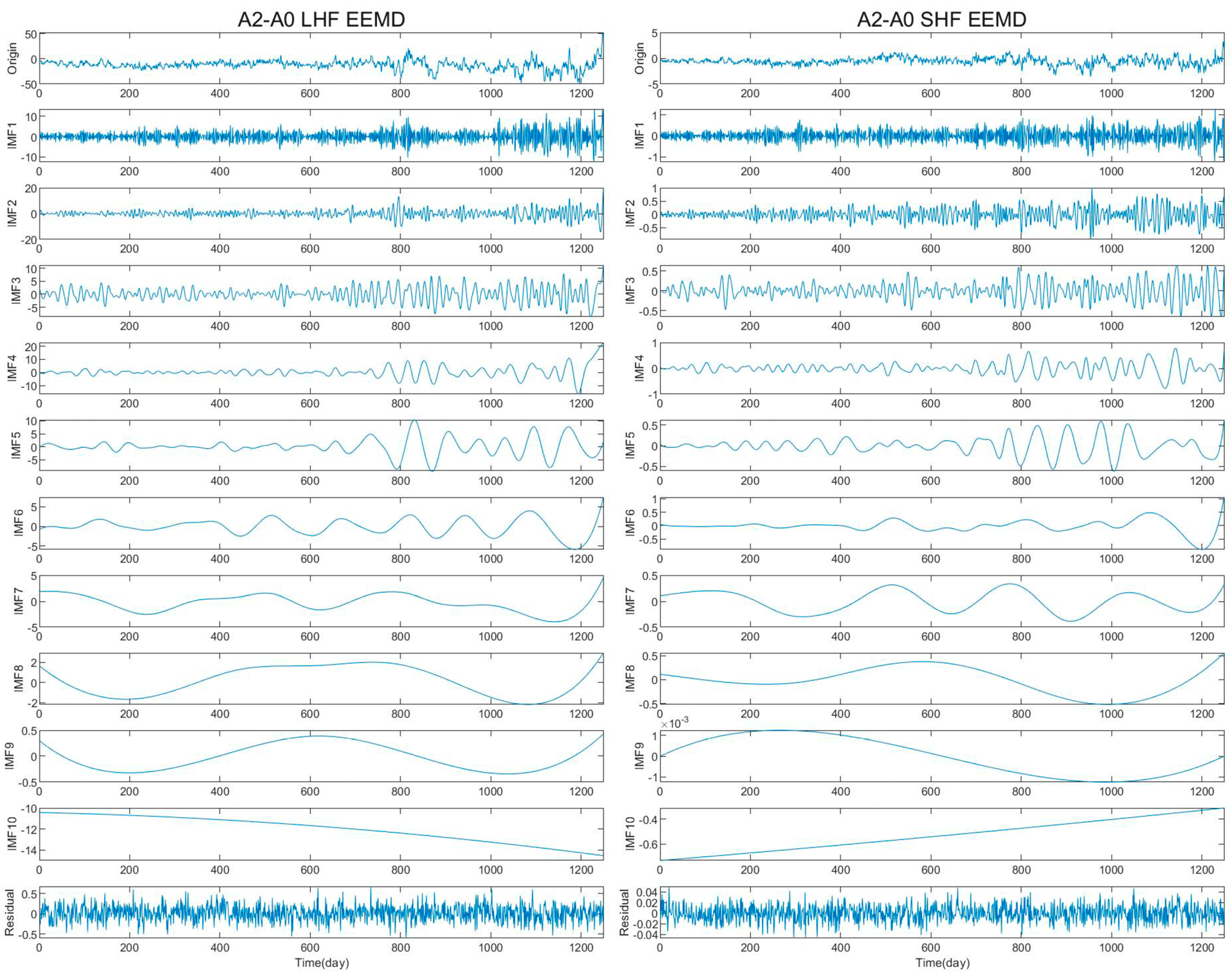
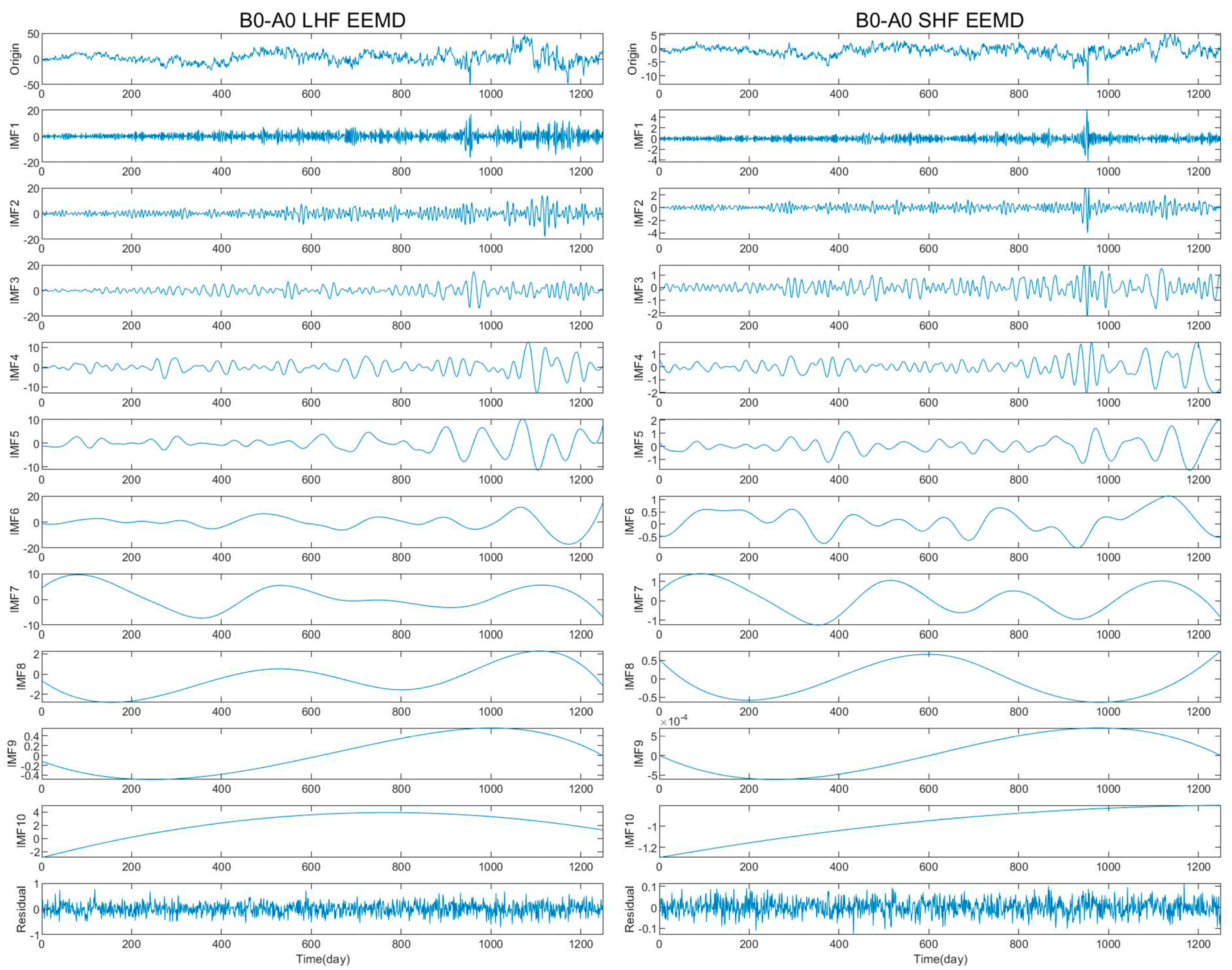
In this section, we evaluate the contributions of the wind speed and other input variables for the estimation of the LHF and SHF based on the COARE 3.5 algorithm at different time scales. First, the ensemble empirical mode decomposition (EEMD) was employed to decompose the time series into intrinsic mode functions (IMFs) with different typical periods [39]. Second, the IMFs of the biases between A1 and A0, A2 and A0, and B0 and A0 were analyzed to quantitatively evaluate the contributions of the wind speed and other input variables.
The EEMD analysis of the turbulent heat flux differences in the global tropical oceans between A1 and A0 are presented in Table 3 (a) and Figure A2. The table displays the average period and contribution to the original signal of each IMF. It can be seen that the periods of each mode for both the LHF and SHF are comparable, and the contributions of the CYGNSS wind speed to the turbulent heat flux differences were mainly in IMF1 and IMF2, which had periods of approximately 3 and 7 days, respectively.
Table 3 (b) and Figure A3 present the EEMD results for the turbulent heat flux difference between A2 and A0, indicating a more scattered contribution of the MERRA-2 wind speed to the difference. The contributions of the LHF difference were concentrated in IMF1 to IMF5, with periods of approximately 3, 8, 15, 40, and 71 days, respectively. Regarding the SHF differences, in addition to the IMF1 and IMF2, IMF8 also made a relatively greater contribution, with a period of about 625 days. These results suggest that different wind speed sets had varying effects on the LHF and SHF differences at various time scales. The variance contribution to the heat flux from the MERRA-2 wind speed was not as prominent as that of the CYGNSS wind speed in IMF1 and IMF2 (Table 3 (b)). This confirms that existing reanalysis products, including MERRA-2, underestimate the impact of the wind speed on the heat flux on time scales shorter than one week, as reported in [40].
3.6. Uncertainty of the Heat Fluxes in Different Ocean Basins
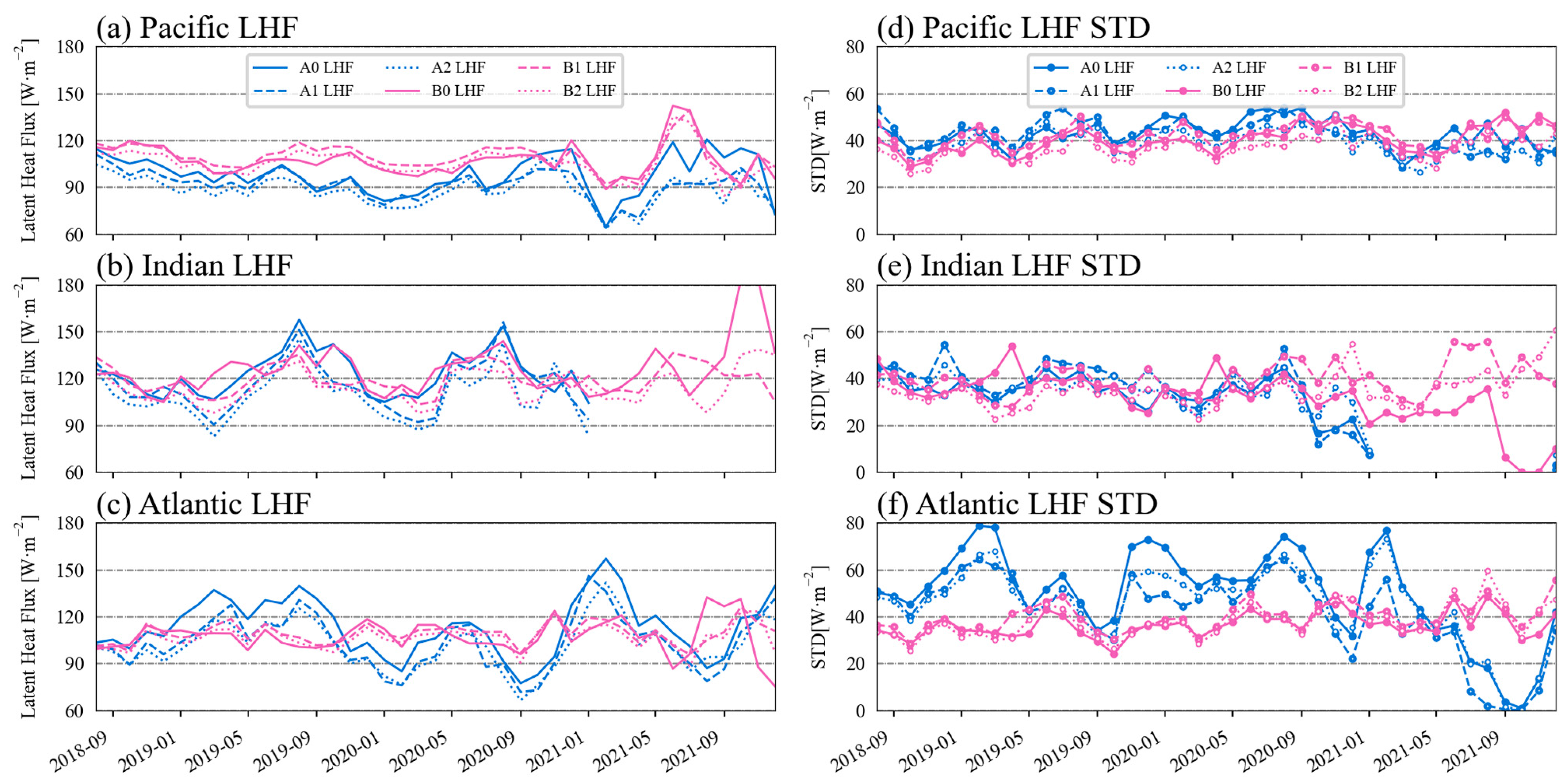
Figure 9 shows the monthly time series of the LHF derived from the experiments listed in Table 2 in the tropical oceans. It can be seen that the LHF of experiments A1 and A2 were generally underestimated compared to that of A0 (Figure 9). In the tropical Pacific Ocean, there was an overall overestimation for the class B experiments compared to the class A experiments, while in the Indian Ocean, there was no substantial overestimation or underestimation for the class B experiments. In the Atlantic Ocean, there was a lower degree of agreement between the variability of the class B and A experiments during the study period. Using A0 as the benchmark, the LHF variation in the Pacific Ocean did not show any obvious seasonal or annual variation characteristics. In contrast, in the Indian Ocean, there was a roughly annual cycle of the LHF variation, which gradually increased from January to August, reaching a yearly maximum in August, and then gradually decreased to a minimum near January. In a previous study [28], a maximum value was found in August each year using one buoy of RAMA and the CYGNSS LHF data. Here, the same finding was found using a total of 20 sites from RAMA in the Indian Ocean. Based on A0, the LHF in the Atlantic Ocean varied drastically, with fluctuation of up to 80 W·m−2 and a relatively weak annual cycle of variation, from near September of each year to a smaller value near September of the following year. Figure 9d–f shows the standard deviation of the LHF for each site in the corresponding month for the ocean. The large standard deviations of the LHF in the Atlantic Ocean for A0 until May 2021 indicate that the LHF in different spatial sites of the Atlantic Ocean varied considerably during that time period.
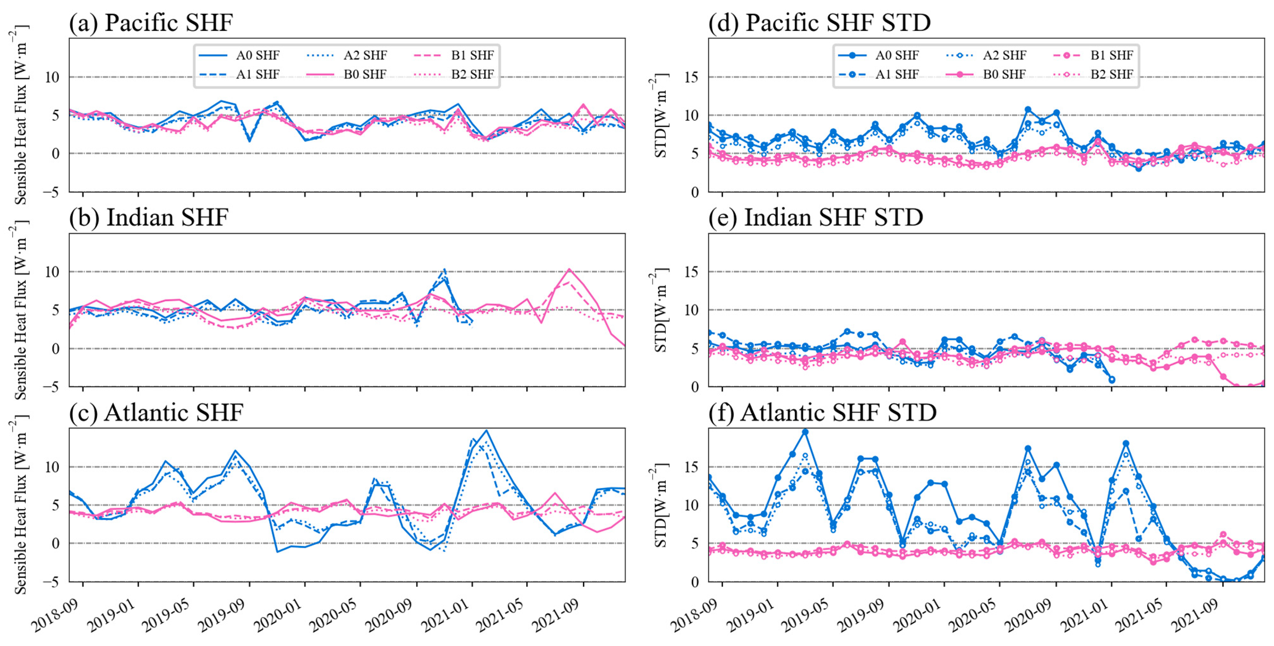
The monthly mean SHF derived from the different experiments generally showed similar variations in the tropical Pacific Ocean (Figure 10a). In the Indian Ocean, the SHF time series of class A and class B were not matched with each other, although they were in good agreement in class A and class B (Figure 10b). Nevertheless, the amplitudes of the SHF were within the same range of 0 to 10 W·m−2 in the Pacific and Indian Oceans. In comparison, the Atlantic SHFs derived from class A showed amplitudes up to 15 W·m−2, roughly three times those of class B. The spatial standard deviation of the SHF in the three oceans are given in Figure 10d–f, showing a flat variation for class B, but a fluctuated variation for class A, respectively. Therefore, in terms of capturing the spatial and temporal variations, it is better to employ other variables from buoy observations for the estimation of the LHF and SHF based on the COARE 3.5 algorithm, particularly in the tropical Atlantic Ocean.
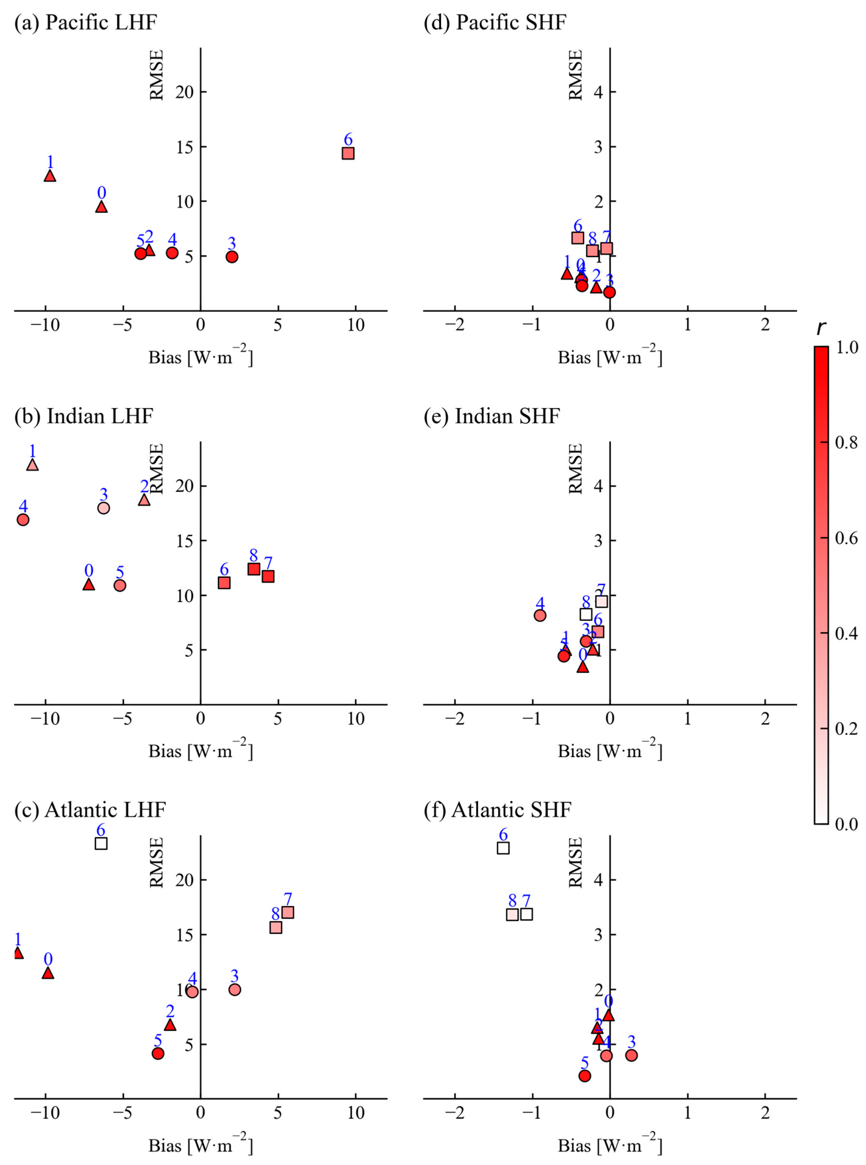
Figure 11 shows the statistical metrics (i.e., RMSE, μ, and r) between the LHF and SHF derived from the six experiments. In the tropical Pacific Ocean, the biases of each pair for the LHF within class A (i.e., between A1 and A0, A2 and A0, and A2 and A1) were from −10 to −4 W m−2, with RMSEs of 5 to 13 W m−2 and correlation coefficients greater than 0.79 (above the 95% significance level). The biases and RMSEs within class B were smaller than those of class A. The biases and RMSEs between class B and A, however, had values greater than 9.5 and 14.4 W m−2 (Figure 11a). These results suggest that the Pacific LHF derived from different input wind speeds with other input variables from buoy observations led to uncertainties smaller than that with the same input wind speeds but different other variables. In comparison, the Pacific LHF derived from different input wind speeds with other input variables from MERRA-2 shows the smallest biases and RMSEs. Similar results can be derived from Figure 11b–f. In the tropical Indian Ocean, the differences in wind speed, rather than other variables, contributed to larger biases and RMSEs for the estimation of the LHF (Figure 11b). In the tropical Atlantic Ocean, both the wind speed and other variables may have induced biases and RMSEs for the estimation of the LHF (Figure 11c). In terms of the SHFs, the biases were generally approximately 10% of the mean values in the tropical Pacific, Indian, and Atlantic Oceans (Figure 11d,f). However, the RMSEs between class B and class A were greater than 3.37 W m−2 with correlation coefficients below the 95% significance level, suggesting that the Atlantic SHF estimation was more sensitive to the input of other variables compared to the wind speed (Figure 11f).
4. Discussion and Conclusions
In Section 3.3, we present the spatial distribution of the biases and RMSEs of the LHF and SHF derived from the CYGNSS and MERRA-2 wind speeds, highlighting areas with relatively large uncertainty. In fact, there have been few studies dedicated to the regional uncertainty evaluation of the CYGNSS and MERRA-2 wind speeds during the study period. Our preliminary speculations are that (1) the large measuring error of the wind speed in these areas has contributed to the biases and RMSEs for deriving the LHF and SHF, and (2) the minor measuring error of the wind speed in these areas may have also contributed to the biases and RMSEs of the LHF and SHF in non-linear computation. Future work could study the uncertainty of the CYGNSS and MERRA-2 wind speeds in these regions and their specific effects on the derivation of turbulent heat fluxes.
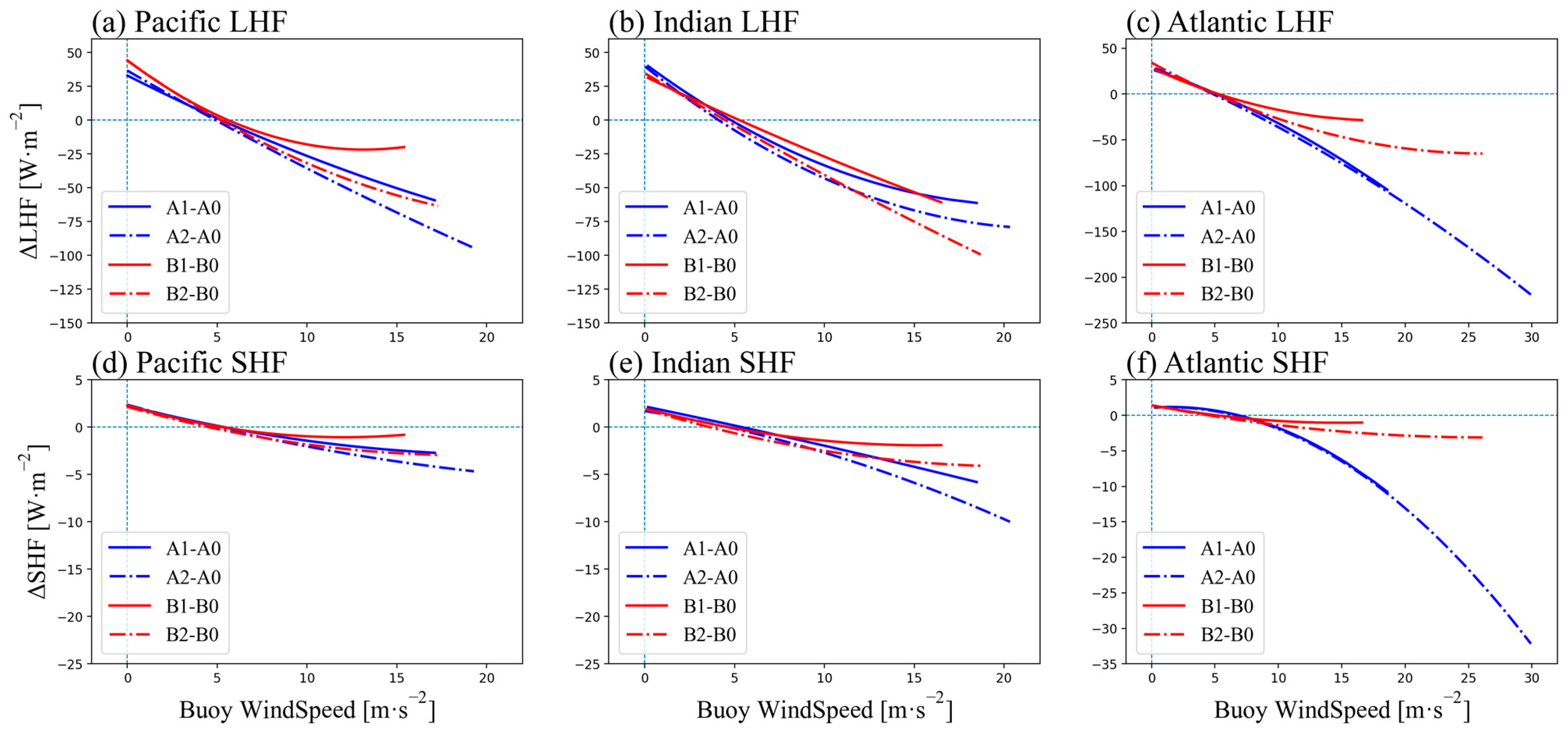
In the previous section, we briefly analyzed the performance of the LHF and SHF for the A0 to B2 experiments in three tropical oceans. Here, we specifically calculate the difference between the heat fluxes calculated by the CYGNSS wind speed and the MERRA-2 wind speed and the heat flux calculated by the buoy wind speed within the three tropical oceans, with respect to the buoy wind speed (Figure 12). Each line in the figure was fitted by matching sample points for the corresponding heat flux differences among the experiments. The results of the quadratic fit without background matching data are presented. All the fitting results show that the LHF and SHF calculated by the two wind speed sets had positive deviations compared to the buoy when the wind speed was less than about 5 m/s. The deviations turned negative when the wind speed exceeded this range, and the deviations increased gradually with the increase in the buoy wind speed. This indicates that the heat fluxes calculated by the CYGNSS and MERRA-2 wind speeds were biased less than the heat fluxes calculated by the buoy wind speed in the high wind speed conditions of the buoy. Previous studies using the CYGNSS wind speed have obtained similar conclusions [26,27]. This is related to the underestimation of the wind speed by CYGNSS in the high wind speed interval. The anomaly of CYGNSS wind retrieval at high wind speeds [29] is also reflected in the calculation of the heat flux. At higher wind speeds, the sensitivity of the ocean surface scattering cross-section to wind speed variations decreases, as does the influence of the hardware parameters. This leads to an increase in errors in the CYGNSS wind retrieval [41,42]. With a sufficient number of matched samples, this trend is more pronounced for A1–A0 and A2–A0 in the Atlantic Ocean, where the differences in the turbulent heat fluxes increased significantly with an increasing buoy wind speed. This indicates that the wind speed differences in the CYGNSS and MERRA-2 compared to those of buoy observations are most pronounced in the Atlantic Ocean. The heat flux differences calculated by B1 and B2 minus B0 were comparatively smaller compared to those calculated by A1 and A2 minus A0. The relatively small differences in the heat fluxes suggest that other state variables are likely to neutralize some of the heat flux differences due to wind speed.
In the Atlantic monthly time series, the class B experiments exhibited more prominent deviations from A0 in the estimation of the LHF and SHF (Figure 9 and Figure 10). Using A0 as a reference, extremes of both the Atlantic LHF and SHF were observed in March and August 2019 and February 2021. This consideration is from the viewpoint of the SST, which affects both the SHF and LHF. However, in the Indian Ocean, extremes appeared only in the LHF, while corresponding extremes did not appear in the SHF, indicating that the SST was not the main cause in the Indian Ocean. It is important to note that the SST is introduced in the calculation of the specific humidity, which is a vital variable in the estimation of the LHF. Although the variability of the SST in the tropical Atlantic has weakened since the turn of the century compared to the last two decades of the previous century, the tropical Atlantic still exhibits a large sea surface temperature anomaly (SSTA) in comparison to other global tropical oceans [43], and the LHF has a strong response to the SSTA [44]. Additionally, larger temperature differences lead to greater humidity differences between the air and sea [45]. Interestingly, the site (34°W, 19°S) with a large LHF deviation in Figure 6 corresponds exactly to the region in [45] where the LHF was the largest in the Atlantic Ocean, suggesting that the LHF derived from the CYGNSS and MERRA-2 wind speeds in this region is biased. It is plausible that the MERRA-2 data may not adequately capture sudden fluctuations in the air temperature, as observed in the case of NCEP reanalysis data. In that particular instance, a rapid decrease in the air temperature during a precipitation event resulted in a significant underestimation of the SHF [46]. The underestimation of the SHF in the Atlantic Ocean, as depicted in Figure 5, could also be attributed to the discrepancies in the sea surface temperature depths between the buoy measurements and the reanalysis data. In this study, both the sea temperature recorded by the buoy (typically at a depth ranging from approximately 0.2 m to 1 m) and the surface skin temperature provided by the reanalysis were utilized as the sea surface temperature indicators. Furthermore, differences in the SST may also be the reason for the significant differences in the LHF and SHF at sites in the Atlantic Ocean (Figure 9f and Figure 10f). Further investigation is necessary to determine the precise impact of the sea and air temperature on the aforementioned issues.
5. Summary
In this study, a set of heat fluxes were calculated based on different combinations of the surface wind, temperature, and humidity by employing the COARE3.5 algorithm. The consistency and differences among the heat fluxes were analyzed based on wavelet coherence analysis and the EEMD method. In addition to the existing studies that have focused on the averaged biases of the CYGNSS heat fluxes in comparison to buoy observations, the new findings of our investigation are as follows:
- (1)
- The turbulent heat fluxes derived from the CYGNSS and MERRA-2 wind speeds show overall consistency with those calculated from buoy wind speed, especially in the high-density matching regions. However, the CYGNSS wind speed had limitations in calculating heat fluxes at high wind speeds, particularly in latent heat flux estimation.
- (2)
- The heat fluxes calculated from the CYGNSS and MERRA-2 wind speeds had differences in the biases and RMSEs when compared to those calculated from buoy winds, mainly at sites located near the equator in the western Pacific Ocean, the Arabian Sea, and the Bay of Bengal, and near the Gulf of Guinea.
- (3)
- The LHF and SHF derived from the CYGNSS showed uncertainty at the synoptic, sub-synoptic and diurnal time scales, and thus, should be further validated before application.
- (4)
- The EEMD results show that the contribution of the CYGNSS wind speed to the LHF and SHF differences can reach a total of 50% and 57% at the high-frequency band, with typical periods of 3–7 days. The MERRA-2 specific humidity had the most significant contribution to the LHF difference in the periods of 192 and 500 days, while its temperature had the largest contribution (16%) to the difference in the SHF in the period of about 1 year.
- (5)
- The monthly LHF and SHF time series in the Pacific and Indian Oceans were generally consistent with each other. However, significant differences were found in the Atlantic Ocean, which may be attributed to the differences in the input SST, rather than the input wind speed.
Author Contributions
Conceptualization, T.X.; methodology, J.L.; software, J.L.; validation, Y.W., H.P., Z.W. and T.X.; formal analysis, J.L.; investigation, J.L.; resources, J.L.; data curation, J.L.; writing—original draft preparation, J.L.; writing—review and editing, Y.W., H.P., Z.W. and T.X.; visualization, J.L.; supervision, Y.W. and T.X.; project administration, Y.W.; funding acquisition, Y.W. and T.X. All authors have read and agreed to the published version of the manuscript.
Funding
This research was jointly funded by the Laoshan Laboratory (Contract No. LSKJ202202700) and the Global Change and Air–Sea Interaction II (Contract No. GASI-01-ATP-STwin). Zexun Wei is supported by the Taishan Scholar Program (No.tstp20221148).
Data Availability Statement
The CYGNSS wind speed data are available at: https://podaac-tools.jpl.nasa.gov/drive/files/allData/cygnss/, accessed on 30 September 2022. The MERRA-2 reanalysis data are available at: https://gmao.gsfc.nasa.gov/reanalysis/MERRA-2/data_access/, accessed on 30 September 2022. The GTMBA buoy data are available at: https://www.pmel.noaa.gov/tao/drupal/disdel/, accessed on 30 September 2022.
Conflicts of Interest
The authors declare no conflict of interest.
Appendix A
Figure A1.
Spatial distribution of biases and RMSEs of LHF and SHF between B1 and B0, and between B2 and B0. Note the color bar of each panel.
Figure A1.
Spatial distribution of biases and RMSEs of LHF and SHF between B1 and B0, and between B2 and B0. Note the color bar of each panel.

Figure A2.
A1-A0, differences of LHF and SHF original daily series and EEMD results.

Figure A3.
A2-A0, differences of LHF and SHF original daily series and EEMD results.

Figure A4.
B0-A0, differences of LHF and SHF original daily series and EEMD results.

References
- Zhang, G.J.; Mcphaden, M.J. The Relationship between Sea Surface Temperature and Latent Heat Flux in the Equatorial Pacific. J. Clim. 1995, 8, 589–605. [Google Scholar] [CrossRef]
- Ma, Z.; Fei, J.; Huang, X.; Cheng, X. Contributions of surface sensible heat fuxes to tropical cyclone. Part I: Evolution of tropical cyclone intensity and structure. J. Atmos. Sci. 2015, 72, 120–140. [Google Scholar] [CrossRef]
- Hsu, C.W.; DeMott, C.A.; Branson, M.D.; Reeves Eyre, J.; Zeng, X. Ocean surface flux algorithm effects on tropical Indo-Pacific intraseasonal precipitation. Geophys. Res. Lett. 2022, 49, e2021GL096968. [Google Scholar] [CrossRef] [PubMed]
- Liu, W.T.; Katsaros, K.B.; Businger, J.A. Bulk Parameterization of Air-Sea Exchanges of Heat and Water Vapor Including the Molecular Constraints at the Interface. J. Atmos. Sci. 1979, 36, 1722–1735. [Google Scholar] [CrossRef]
- Fairall, C.W.; Bradley, E.F.; Rogers, D.P.; Edson, J.B.; Young, G.S. Bulk parameterization of air-sea fluxes for Tropical Ocean-Global Atmosphere Coupled-Ocean Atmosphere Response Experiment. J. Geophys. Res. Ocean. 1996, 101, 3747–3764. [Google Scholar] [CrossRef] [Green Version]
- Edson, J.B.; Jampana, V.; Weller, R.A.; Bigorre, S.P.; Plueddemann, A.J.; Fairall, C.W.; Miller, S.D.; Mahrt, L.; Vickers, D.; Hersbach, H. On the exchange of momentum over the open ocean. J. Phys. Oceanogr. 2013, 43, 1589–1610. [Google Scholar] [CrossRef] [Green Version]
- Cronin, M.F.; Gentemann, C.L.; Edson, J.; Ueki, I.; Bourassa, M.; Brown, S.; Clayson, C.A.; Fairall, C.W.; Farrar, J.T.; Gille, S.T.; et al. Air-sea fluxes with a focus on heat and momentum. Front. Mar. Sci. 2019, 6, 430. [Google Scholar] [CrossRef] [Green Version]
- Bentamy, A.; Piolle, J.F.; Grouazel, A.; Danielson, R.; Gulev, S.; Paul, F.; Azelmat, H.; Mathieu, P.; von Schuckmann, K.; Sathyendranath, S.; et al. Review and assessment of latent and sensible heat flux accuracy over the global oceans. Remote Sens. Environ. 2017, 201, 196–218. [Google Scholar] [CrossRef] [Green Version]
- Tomita, H.; Kubota, M.; Cronin, M.F.; Iwasaki, S.; Konda, M.; Ichikawa, H. An assessment of surface heat fluxes from J-OFURO2 at the KEO and JKEO sites. J. Geophys. Res. Ocean. 2010, 115, C03018. [Google Scholar] [CrossRef] [Green Version]
- Tomita, H.; Hihara, T.; Kako, S.; Kubota, M.; Kutsuwada, K. An introduction to J-OFURO3, a third-generation Japanese ocean flux data set using remote-sensing observations. J. Oceanogr. 2019, 75, 171–194. [Google Scholar] [CrossRef] [Green Version]
- Roberts, J.B.; Robertson, F.R.; Clayson, C.A.; Bosilovich, M.G. Characterization of turbulent latent and sensible heat flux exchange between the atmosphere and ocean in MERRA. J. Clim. 2012, 25, 821–838. [Google Scholar] [CrossRef] [Green Version]
- Al Senafi, F.; Anis, A.; Menezes, V. Surface Heat Fluxes over the Northern Arabian Gulf and the Northern Red Sea: Evaluation of ECMWF-ERA5 and NASA-MERRA2 Reanalyses. Atmosphere 2019, 10, 504. [Google Scholar] [CrossRef] [Green Version]
- Decker, M.; Brunke, M.A.; Wang, Z.; Sakaguchi, K.; Zeng, X.; Bosilovich, M.G. Evaluation of the Reanalysis Products from GSFC, NCEP, and ECMWF Using Flux Tower Observations. J. Clim. 2012, 25, 1916–1944. [Google Scholar] [CrossRef]
- Josey, S.A.; Yu, L.; Gulev, S.; Jin, X.; Tilinina, N.; Barnier, B.; Brodeau, L. Unexpected impacts of the Tropical Pacific array on reanalysis surface meteorology and heat fluxes. Geophys. Res. Lett. 2014, 41, 6213–6220. [Google Scholar] [CrossRef] [Green Version]
- Valdivieso, M.; Haines, K.; Balmaseda, M.; Chang, Y.-S.; Drevillon, M.; Ferry, N.; Fujii, Y.; Koehl, A.; Storto, A.; Toyoda, T.; et al. An assessment of air–sea heat fluxes from ocean and coupled reanalyses. Clim. Dyn. 2017, 49, 983–1008. [Google Scholar] [CrossRef] [Green Version]
- Huang, B.; Liu, C.; Ren, G.; Zhang, H.; Zhang, L. The Role of Buoy and Argo Observations in Two SST Analyses in the Global and Tropical Pacific Oceans. J. Clim. 2019, 32, 2517–2535. [Google Scholar] [CrossRef]
- Tomita, H.; Kutsuwada, K.; Kubota, M.; Hihara, T. Advances in the estimation of global surface net heat flux based on satellite observation: J-OFURO3 V1.1. Front. Mar. Sci. 2021, 8, 612361. [Google Scholar] [CrossRef]
- Pokhrel, S.; Dutta, U.; Rahaman, H.; Chaudhari, H.; Hazra, A.; Saha, S.K.; Veeranjaneyulu, C. Evaluation of different heat flux products over the tropical Indian Ocean. Earth Space Sci. 2020, 7, e2019EA000988. [Google Scholar] [CrossRef] [Green Version]
- Carvalho, D.; Rocha, A.; Gómez-Gesteira, M.; Santos, C.S. Comparison of reanalyzed, analyzed, satellite-retrieved and NWP modelled winds with buoy data along the Iberian Peninsula coast. Remote Sens. Environ. 2014, 152, 480–492. [Google Scholar] [CrossRef]
- Tomita, H.; Hihara, T.; Kubota, M. Improved satellite estimation of near-surface humidity using vertical water vapor profile information. Geophys. Res. Lett. 2018, 45, 899–906. [Google Scholar] [CrossRef]
- Robertson, F.R.; Roberts, J.B.; Bosilovich, M.G.; Bentamy, A.; Clayson, C.A.; Fennig, K.; Schröder, M.; Tomita, H.; Compo, G.P.; Gutenstein, M.; et al. Uncertainties in Ocean Latent Heat Flux Variations over Recent Decades in Satellite-Based Estimates and Reduced Observation Reanalyses. J. Clim. 2020, 33, 8415–8437. [Google Scholar] [CrossRef]
- Tomita, H.; Kubota, M. An analysis of the accuracy of Japanese Ocean Flux data sets with Use of Remote sensing Observations (J-OFURO) satellite-derived latent heat flux using moored buoy data. J. Geophys. Res. Ocean. 2006, 111, C07007. [Google Scholar] [CrossRef] [Green Version]
- Ruf, C.S.; Atlas, R.; Chang, P.S.; Clarizia, M.P.; Garrison, J.L.; Gleason, S.; Katzberg, S.J.; Jelenak, Z.; Johnson, J.T.; Majumdar, S.J.; et al. New Ocean Winds Satellite Mission to Probe Hurricanes and Tropical Convection. Bull. Am. Meteorol. Soc. 2016, 97, 385–395. [Google Scholar] [CrossRef]
- Asharaf, S.; Waliser, D.E.; Posselt, D.J.; Ruf, C.S.; Zhang, C.; Putra, A.W. CYGNSS ocean surface wind validation in the tropics. J. Atmos. Ocean. Technol. 2021, 38, 711–724. [Google Scholar] [CrossRef]
- Yi, Y.; Johnson, J.T.; Wang, X. Diurnal Variations in Ocean Wind Speeds Measured by CYGNSS and Other Satellites. IEEE Geosci. Remote Sens. Lett. 2021, 19, 1–5. [Google Scholar] [CrossRef]
- Crespo, J.A.; Posselt, D.J.; Asharaf, S. CYGNSS Surface Heat Flux Product Development. Remote Sens. 2019, 11, 2294. [Google Scholar] [CrossRef] [Green Version]
- Lin, J.; Wang, Y.; Xu, T. CYGNSS Sea Surface Heat Flux Product Validation and Its Applicability. In Proceedings of the OCEANS 2022 Hampton Roads, Hampton Roads, VA, USA, 17–20 October 2022; IEEE: New York, NY, USA, 2022; pp. 1–6. [Google Scholar] [CrossRef]
- Li, X.; Yang, J.; Yan, Y.; Li, W. Exploring CYGNSS mission for surface heat flux estimates and analysis over tropical oceans. Front. Mar. Sci. 2022, 9, 1001491. [Google Scholar] [CrossRef]
- Li, X.; Yang, D.; Yang, J.; Han, G.; Zheng, G.; Li, W. Validation of NOAA CyGNSS Wind Speed Product with the CCMP Data. Remote Sens. 2021, 13, 1832. [Google Scholar] [CrossRef]
- Ricciardulli, L.; Mears, C.; Manaster, A.; Meissner, T. Assessment of CYGNSS Wind Speed Retrievals in Tropical Cyclones. Remote Sens. 2021, 13, 5110. [Google Scholar] [CrossRef]
- Hammond, M.L.; Foti, G.; Gommenginger, C.; Srokosz, M. An Assessment of CyGNSS v3.0 Level 1 Observables over the Ocean. Remote Sens. 2021, 13, 3500. [Google Scholar] [CrossRef]
- Brunke, M.A.; Zeng, X.; Anderson, S. Uncertainties in sea surface turbulent flux algorithms and data sets. J. Geophys. Res. Ocean. 2002, 107, 3141. [Google Scholar] [CrossRef] [Green Version]
- Fairall, C.W.; Bradley, E.F.; Hare, J.E.; Grachev, A.A.; Edson, J.B. Bulk parameterization of air-sea fluxes: Updates and verification for the COARE algorithm. J. Clim. 2003, 16, 571–591. [Google Scholar] [CrossRef]
- Brunke, M.A.; Fairall, C.W.; Zeng, X.; Eymard, L.; Curry, J.A. Which Bulk Aerodynamic Algorithms are Least Problematic in Computing Ocean Surface Turbulent Fluxes? J. Clim. 2003, 16, 619–635. [Google Scholar] [CrossRef]
- Rienecker, M.M.; Suarez, M.J.; Gelaro, R.; Todling, R.; Bacmeister, J.; Liu, E.; Bosilovich, M.G.; Schubert, S.D.; Takacs, L.; Kim, G.-K.; et al. MERRA: NASA’s Modern-Era Retrospective Analysis for Research and Applications. J. Clim. 2011, 24, 3624–3648. [Google Scholar] [CrossRef]
- Global Modeling and Assimilation Office (GMAO). MERRA-2 tavg1_2d_flx_Nx: 2d,1-Hourly, Time-Averaged, Single-Level, Assimilation, Surface Flux Diagnostics V5.12.4; Goddard Earth Sciences Data and Information Services Center (GES DISC): Greenbelt, MD, USA, 2015. [CrossRef]
- Global Modeling and Assimilation Office (GMAO). MERRA-2 tavg1_2d_slv_Nx: 2d,1-Hourly, Time-Averaged, Single-Level, Assimilation, Single-Level Diagnostics V5.12.4; Goddard Earth Sciences Data and Information Services Center (GES DISC): Greenbelt, MD, USA, 2015. [CrossRef]
- Grinsted, A.; Moore, J.C.; Jevrejeva, S. Application of the cross wavelet transform and wavelet coherence to geophysical time series. Nonlinear Proc. Geophys. 2004, 11, 561–566. [Google Scholar] [CrossRef]
- Wu, Z.; Huang, N.E. Ensemble empirical mode decomposition: A noise-assisted data analysis method. Adv. Adapt. Data Anal. 2009, 1, 1–41. [Google Scholar] [CrossRef]
- Yan, Y.; Song, X.; Wang, G.; Chen, C. Importance of high-frequency (≤30-day) wind variability to the annual climatology of the surface latent heat flux inferred from the global tropical moored buoy array. J. Geophys. Res. Ocean. 2022, 127, e2021JC018094. [Google Scholar] [CrossRef]
- Ruf, C.S.; Gleason, S.; McKague, D.S. Assessment of CYGNSS wind speed retrieval uncertainty. IEEE J-STARS 2018, 12, 87–97. [Google Scholar] [CrossRef]
- Clarizia, M.P.; Ruf, C.S. Statistical derivation of wind speeds from CYGNSS data. IEEE Trans. Geosci. Remote Sens. 2020, 58, 3955–3964. [Google Scholar] [CrossRef]
- Prigent, A.; Lübbecke, J.F.; Bayr, T.; Latif, M.; Wengel, C. Weakened SST variability in the tropical Atlantic Ocean since 2000. Clim. Dyn. 2020, 54, 2731–2744. [Google Scholar] [CrossRef]
- Ren, H.; Zuo, J.; Li, W. The Impact of Tropical Atlantic SST Variability on the Tropical Atmosphere during Boreal Summer. J. Clim. 2021, 34, 6705–6723. [Google Scholar] [CrossRef]
- Leyba, I.M.; Solman, S.A.; Saraceno, M. Trends in sea surface temperature and air–sea heat fluxes over the South Atlantic Ocean. Clim. Dyn. 2019, 53, 4141–4153. [Google Scholar] [CrossRef]
- Swain, D.; Rahman, S.H.; Ravichandran, M. Comparison of NCEP turbulent heat fluxes with in situ observations over the south-eastern Arabian Sea. Meteorol. Atmos. Phys. 2009, 104, 163–175. [Google Scholar] [CrossRef]
Figure 1.
Locations of buoys selected from the Global Tropical Moored Buoy Array. Dark green solid circles represent RAMA buoys with complete input variables, and dark green hollow circles represent RAMA buoys with only missing SLP data. The red solid and hollow circles are the corresponding TAO buoys, and the orange solid and hollow circles are the corresponding PIRATA buoys.

Figure 2.
Experimental design and flow chart.

Figure 3.
LHF and SHF matched scatter density plot of experiments A and B. (a–d) Comparisons of A1 and A2 with A0. (e–h) Comparisons of B1 and B2 with B0, respectively. RMSE: root mean square error, unit: W·m−2; µ: mean bias, unit: W·m−2; r: correlation coefficient; N: number of samples.
Figure 3.
LHF and SHF matched scatter density plot of experiments A and B. (a–d) Comparisons of A1 and A2 with A0. (e–h) Comparisons of B1 and B2 with B0, respectively. RMSE: root mean square error, unit: W·m−2; µ: mean bias, unit: W·m−2; r: correlation coefficient; N: number of samples.

Figure 4.
Correlation coefficient (red solid line) and RMSE (blue dashed line) distributions refer to different LHF or SHF ranges. Gray bars indicate the percentages of the sample numbers within the LHF or SHF ranges of the total sample numbers.
Figure 4.
Correlation coefficient (red solid line) and RMSE (blue dashed line) distributions refer to different LHF or SHF ranges. Gray bars indicate the percentages of the sample numbers within the LHF or SHF ranges of the total sample numbers.

Figure 5.
LHF and SHF derived from the experiments listed in Table 2 in the tropical Pacific, Indian, and Atlantic Oceans. Solid dots are the area-averaged values of the period from 1 August 2018 to 31 December 2021, and bars are the spatial standard deviations.
Figure 5.
LHF and SHF derived from the experiments listed in Table 2 in the tropical Pacific, Indian, and Atlantic Oceans. Solid dots are the area-averaged values of the period from 1 August 2018 to 31 December 2021, and bars are the spatial standard deviations.

Figure 6.
Spatial distribution of biases and RMSEs in LHF and SHF between A1 and A0, and between A2 and A0. Note the color bar of each panel.
Figure 6.
Spatial distribution of biases and RMSEs in LHF and SHF between A1 and A0, and between A2 and A0. Note the color bar of each panel.

Figure 7.
Wavelet coherence of LHF between (a) A1 and A0, (b) A2 and A0, (c) B0 and A0, (d) B1 and A1, and (e) B2 and A2. The horizontal axis is time and the vertical axis is period. The yellow shadings are above the 95% significance level. The rightward and leftward arrows indicate that the time series are in phase and out of phase, respectively, whereas the upward and downward arrows indicate that the time series are in half-phase lag.

Figure 8.
Same as Figure 7, but for the SHF.
Figure 8.
Same as Figure 7, but for the SHF.

Figure 9.
Monthly time series of the LHF derived from the experiments listed in Table 2 in the tropical (a) Pacific, (b) Indian, and (c) Atlantic Oceans, as well as the corresponding spatial standard deviation in the tropical (d) Pacific, (e) Indian, and (f) Atlantic Oceans.
Figure 9.
Monthly time series of the LHF derived from the experiments listed in Table 2 in the tropical (a) Pacific, (b) Indian, and (c) Atlantic Oceans, as well as the corresponding spatial standard deviation in the tropical (d) Pacific, (e) Indian, and (f) Atlantic Oceans.

Figure 10.
Same as Figure 9, but for the SHF.
Figure 10.
Same as Figure 9, but for the SHF.

Figure 11.
Statistical metrics of different pairs of the LHF and SHF derived from the experiments listed in Table 2 in the tropical Pacific, Indian, and Atlantic Oceans. Triangles, circles, and squares represent those within class A (marked as blue numerals 0, 1, and 2), within class B (marked as blue numerals 3, 4, and 5), and between A and B (marked as blue numerals 6, 7, and 8), respectively. The pairs are classified as: 0 (A1–A0), 1 (A2–A0), 2 (A2–A1), 3 (B1–B0), 4 (B2–B0), 5 (B2–B1), 6 (B0–A0), 7 (B1–A1), and 8 (B2–A2).

Figure 12.
Differences of LHF and SHF vary with buoy wind speed.


Table 1.
MERRA-2 data selection. The M2T1NXSLV only provided surface skin temperature, which was adopted as sea surface temperature following previous investigations [26,28].
| Data Collection | Variable | Spatial Res | Temporal Res | Spatial Coverage | Time Span |
|---|---|---|---|---|---|
| M2T1NXFLX | 𝜌𝑎, 𝑞𝑠 | 0.625° × 0.5° | 1 h from 00:30 UTC | 40°S~40°N | 1 August 2018~31 December 2021 |
| M2T1NXSLV | 𝑞a, SLP, 𝑇𝑠, 𝑇𝑎, 𝑈 |
Table 2.
Description of experiments and variables.
| Experiments | Output Variables | Input Variables | ||
|---|---|---|---|---|
| Description | Symbol | Wind Speed | Other Variables | |
| Buoy Original | A0 | LHFA0 SHFA0 | 𝑈Buoy | 𝑇𝑎 Buoy 𝑇𝑠 Buoy 𝑞a Buoy 𝑞𝑠 Buoy 𝜌𝑎 Buoy |
| CYGNSS Wind + Buoy Variable | A1 | LHFA1 SHFA1 | 𝑈CYGNSS | |
| MERRA-2 Wind + Buoy Variable | A2 | LHFA2 SHFA2 | 𝑈MERRA2 | |
| Buoy Wind + MERRA-2 Variable | B0 | LHFB0 SHFB0 | 𝑈Buoy | 𝑇𝑎 MERRA2 𝑇𝑠 MERRA2 𝑞a MERRA2 𝑞𝑠 MERRA2 ρa MERRA2 |
| CYGNSS Wind + MERRA-2 Variable | B1 | LHFB1 SHFB1 | 𝑈CYGNSS | |
| MERRA-2 Wind + MERRA-2 Variable | B2 | LHFB2 SHFB2 | 𝑈MERRA2 | |
Table 3.
Mean period (unit in days), variance (unit in W2·m−4), and contributions of the IMFs based on the differences in the LHF and SHF derived from different inputs of wind speed and other variables using the COARE 3.5 algorithm.
Table 3.
Mean period (unit in days), variance (unit in W2·m−4), and contributions of the IMFs based on the differences in the LHF and SHF derived from different inputs of wind speed and other variables using the COARE 3.5 algorithm.
| (a) A1–A0 Turbulent Heat Fluxes, EEMD | ||||||
| IMF | LHF | SHF | ||||
| Mean Period | IMFs Variance | Contribution | Mean Period | IMFs Variance | Contribution | |
| 1 | 2.9562 | 39.8189 | 31.48% | 2.9667 | 0.9454 | 40.69% |
| 2 | 6.9197 | 23.3616 | 18.47% | 6.3887 | 0.3762 | 16.19% |
| 3 | 13.2169 | 11.3026 | 8.93% | 14.3563 | 0.2314 | 9.96% |
| 4 | 27.4505 | 8.2958 | 6.56% | 26.0208 | 0.1382 | 5.95% |
| 5 | 65.7368 | 9.389 | 7.42% | 55.5111 | 0.1017 | 4.37% |
| 6 | 124.9 | 1.8314 | 1.45% | 113.5455 | 0.0469 | 2.02% |
| 7 | 416.3333 | 1.6232 | 1.28% | 356.8571 | 0.0816 | 3.51% |
| 8 | 624.5 | 3.4955 | 2.76% | 624.5 | 0.0581 | 0.25% |
| (b) A2–A0 Turbulent Heat Fluxes, EEMD | ||||||
| IMF | LHF | SHF | ||||
| Mean Period | IMFs Variance | Contribution | Mean Period | IMFs Variance | Contribution | |
| 1 | 3.2868 | 9.7569 | 10.22% | 3.1701 | 0.0987 | 17.85% |
| 2 | 7.8801 | 8.9691 | 9.4% | 7.0765 | 0.057 | 10.31% |
| 3 | 15.2317 | 6.7156 | 7.04% | 14.6941 | 0.0421 | 7.62% |
| 4 | 38.4308 | 17.6207 | 18.46% | 30.4634 | 0.0511 | 9.24% |
| 5 | 71.3714 | 9.2526 | 9.69% | 62.45 | 0.0446 | 8.06% |
| 6 | 146.9412 | 3.969 | 4.16% | 156.125 | 0.0531 | 0.96% |
| 7 | 416.3333 | 2.3369 | 2.45% | 312.25 | 0.0396 | 7.16% |
| 8 | 624.5 | 1.8754 | 1.96% | 624.5 | 0.0748 | 13.53% |
| (c) B0–A0 Turbulent Heat Fluxes, EEMD | ||||||
| IMF | LHF | SHF | ||||
| Mean Period | IMFs Variance | Contribution | Mean Period | IMFs Variance | Contribution | |
| 1 | 3.3086 | 11.4619 | 8.92% | 3.313 | 0.3726 | 10.85% |
| 2 | 7.7337 | 10.0341 | 7.81% | 7.6391 | 0.2825 | 8.23% |
| 3 | 16.8784 | 9.4895 | 7.39% | 15.5155 | 0.2504 | 7.29% |
| 4 | 35.1831 | 9.1559 | 7.13% | 35.1831 | 0.4092 | 11.92% |
| 5 | 75.697 | 11.0604 | 8.61% | 69.3889 | 0.3671 | 10.69% |
| 6 | 192.1538 | 29.6947 | 23.11% | 208.1667 | 0.2131 | 6.21% |
| 7 | 499.6 | 18.1702 | 14.14% | 356.8571 | 0.5524 | 16.09% |
| 8 | 624.5 | 1.2988 | 1.01% | 624.5 | 0.1915 | 5.58% |
Disclaimer/Publisher’s Note: The statements, opinions and data contained in all publications are solely those of the individual author(s) and contributor(s) and not of MDPI and/or the editor(s). MDPI and/or the editor(s) disclaim responsibility for any injury to people or property resulting from any ideas, methods, instructions or products referred to in the content. |
© 2023 by the authors. Licensee MDPI, Basel, Switzerland. This article is an open access article distributed under the terms and conditions of the Creative Commons Attribution (CC BY) license (https://creativecommons.org/licenses/by/4.0/).
Share and Cite
MDPI and ACS Style
Lin, J.; Wang, Y.; Pan, H.; Wei, Z.; Xu, T. Uncertainty of CYGNSS-Derived Heat Flux Variations at Diurnal to Seasonal Time Scales over the Tropical Oceans. Remote Sens. 2023, 15, 3161. https://doi.org/10.3390/rs15123161
AMA Style
Lin J, Wang Y, Pan H, Wei Z, Xu T. Uncertainty of CYGNSS-Derived Heat Flux Variations at Diurnal to Seasonal Time Scales over the Tropical Oceans. Remote Sensing. 2023; 15(12):3161. https://doi.org/10.3390/rs15123161
Chicago/Turabian StyleLin, Jinsong, Yanfeng Wang, Haidong Pan, Zexun Wei, and Tengfei Xu. 2023. "Uncertainty of CYGNSS-Derived Heat Flux Variations at Diurnal to Seasonal Time Scales over the Tropical Oceans" Remote Sensing 15, no. 12: 3161. https://doi.org/10.3390/rs15123161
Note that from the first issue of 2016, this journal uses article numbers instead of page numbers. See further details here.