

Robust LiDAR-Based Vehicle Detection for On-Road Autonomous Driving

1
School of Mechatronic Engineering and Automation, Shanghai Key Laboratory of Intelligent Manufacturing and Robotics, Shanghai University, Shanghai 200072, China
2
State Key Laboratory of Automotive Simulation and Control, Jilin University, Changchun 130025, China
3
College of Agricultural Unmanned System, China Agricultural University, Beijing 100193, China
4
College of Science, China Agricultural University, Beijing 100193, China
5
Shanghai Tenghao Vision Technology Limited Company, Shanghai 201107, China
*
Author to whom correspondence should be addressed.
Remote Sens. 2023, 15(12), 3160; https://doi.org/10.3390/rs15123160
Submission received: 29 May 2023
/
Revised: 12 June 2023
/
Accepted: 15 June 2023
/
Published: 17 June 2023
(This article belongs to the Special Issue Remote Sensing in Civil and Environmental Engineering)
Abstract
:The stable detection and tracking of high-speed vehicles on the road by using LiDAR can input accurate information for the decision-making module and improve the driving safety of smart cars. This paper proposed a novel LiDAR-based robust vehicle detection method including three parts: point cloud clustering, bounding box fitting and point cloud recognition. Firstly, aiming at the problem of clustering quality degradation caused by the uneven distribution of LiDAR point clouds and the difference in clustering radius between point cloud clusters in traditional DBSCAN (TDBSCAN) obstacle clustering algorithms, an improved DBSCAN algorithm based on distance-adaptive clustering radius (ADBSCAN) is designed, and a point cloud KD-Tree data structure is constructed to speed up the traversal of the algorithm; meanwhile, the OPTICS algorithm is introduced to enhance the performance of the proposed algorithm. Then, by adopting different fitting strategies for vehicle contour points in various states, the adaptability of the bounding box fitting algorithm is improved; Moreover, in view of the shortcomings of the poor robustness of the L-shape algorithm, the principal component analysis method (PCA) is introduced to obtain stable bounding box fitting results. Finally, considering the time-consuming and low-accuracy training of traditional machine learning algorithms, advanced PointNet in deep learning technique is built to send the point cloud within the bounding box of a high-confidence vehicle into PointNet to complete vehicle recognition. Experiments based on our autonomous driving perception platform and the KITTI dataset prove that the proposed method can stably complete vehicle target recognition and achieve a good balance between time-consuming and accuracy.
1. Introduction
1.1. Background
Driverless technology of intelligent vehicles has received extensive attention and research in recent years [1,2,3,4,5,6,7,8,9]. According to United Nations statistics, road accidents kill 1.3 million people and injure 50 million people worldwide every year; the emergence of autonomous driving technology can effectively avoid some accidents and improve road safety. Environmental perception technology is the first link of autonomous driving, and the use of LiDAR to stably detect high-speed vehicles on the road can input accurate information for the decision-making module and improve the driving safety of intelligent vehicles. Therefore, ensuring stable detection of vehicle targets plays a decisive role in the development of driverless technology.
The visual perception scheme obtains vehicle semantic information by collecting rich RGB information and infers vehicle location information. However, under special working conditions such as rain, snow, fog and night, the detection accuracy of the visual perception scheme will drop significantly or even fail; in contrast, LiDAR acquires point clouds by emitting laser light and receiving reflected signals. Processing point cloud data can directly obtain rich information such as the shape, position and orientation of the vehicle. In addition, the lidar can still work normally in bad weather or at night, effectively avoiding the algorithm failure of the camera caused by bad weather or insufficient light.
1.2. Related Research
At present, vehicle detection technology based on LiDAR is mainly divided into vehicle detection algorithms based on point cloud segmentation and vehicle detection algorithms based on point cloud classification [1]. The vehicle detection algorithm based on point cloud segmentation is supported by point cloud convolutional neural networks. By extracting features from the scattered and disordered point cloud of the input, it can segment the ground, pedestrians, or other obstacles in the out-point cloud while obtaining the vehicle target. The vehicle detection algorithm based on point cloud classification is called the traditional algorithm compared with neural networks which follows three processes: drivable area detection, point cloud clustering and point cloud classification.
Recently, some efforts of deep learning-based vehicle detection have been brought forward in this respect. Xia et al. [5] presented an automated driving system data acquisition and analytics platform through a deep-learning-based object detection algorithm using LiDAR information, a late fusion scheme to leverage cooperative perception from multi-connected automated vehicles is introduced. Liu et al. [6] proposed a novel YOLOv5-tassel algorithm with a bidirectional feature pyramid network to detect tassels, annotation is performed with guidance from center points derived from CenterNet to improve the selection of the bounding boxes for tassels. Monisha et al. [7] investigated an efficient relay node selection scheme for mission critical communication using machine learning, the temporary database learning and control (t-DLC) unit during an emergency is attached to minimize communication overhead in the medium. Kingston Roberts et al. [8] designed an improved optimal energy-aware data availability approach for secure clustering and routing in wireless sensor networks, it can increase the network lifetime by focusing on the selection of stable routing paths and cluster heads. So et al. [9] analyzed the probability of visibility limitation of autonomous vehicle detection performance according to various road geometry settings, and the reliable autonomous driving system will improve traffic safety based on the enhanced detection and recognition capability of autonomous vehicle sensors. YOLO3D [10] uses the average value of each category label box as the size of the 3D prior box and inputs the maximum height feature map and density feature map into the YOLOV2 network structure for classification tasks and regression, and this method is simple and efficient. Compared with the 2D classification task, only the height information z, the height dimension h and the prediction of the direction θ are added. Pixor [11] does not consider height and density features when constructing feature maps but only considers occupancy and reflectivity. By constructing feature maps under the top view, and then extracting features through 2D CNN. PointNet [12] is a deep learning framework for point cloud classification and segmentation proposed by Stanford University in 2017. Due to the irregular spatial relationship of the point cloud during classification or segmentation, the existing image classification and segmentation framework cannot be directly applied to the point cloud. PointNet uses the input method of the original point cloud and extracts the point cloud by designing 1024-dimensional features, and then it performs maximum pooling on each dimension of the features and utilizes two fully connected layers to complete point cloud classification or segmentation after obtaining global features. PointNet preserves the spatial characteristics of the point cloud to the greatest extent, and it can achieve good results in the final test. Considering that voxel-based methods can efficiently encode multi-scale feature representations and generate high-quality 3D proposal boxes, and raw point-based methods can also preserve more precise location information, Shi et al. [13] proposed a novel 3D object Detection framework PV-RCNN, the method first uses 3D Voxel CNN to divide the scene into (L, W and H) voxels, and then utilizes the SA operation proposed in PointNet++ to aggregate voxel features at different scales. Li et al. [14] proposed a fast and general-purpose two-stage 3D detector LiDAR R-CNN, this method uses a common voxelization method for detection and applies the original point cloud information to obtain a more accurate image after removing most of the background. For the bounding box, the number of point clouds in the classification stage is greatly reduced due to the deletion of background points. The second-stage network can perfectly avoid the shortcomings of point-based methods with large calculations while retaining the precise geometry of the target in the original point cloud.
Moreover, note that VoxelNet [15] voxelizes the original point cloud for random sampling, then uses the voxel feature encoding layer (Voxel Feature Encode) for feature extraction, and finally the region generation network RPN (Region Proposal) is exploited to complete the classification and segmentation. Based on VoxelNet, Yan [16] proposed a spatially sparse convolutional network with SSD as the detection head which has improved speed and accuracy. PointPillars can improve the point cloud representation based on VoxelNet, which converts point clouds into fake images and then achieves target detection through 2D convolution. Voxel rcnn [17] treats a sparse but regular 3D volume as a set of non-empty voxel center points and utilizes an accelerated PointNet module to achieve a new balance between accuracy and efficiency.
The vehicle detection algorithm based on point cloud segmentation needs to rely on a large amount of training data sets, resulting in poor transferability in different scenarios and difficulty in landing. The technical route of the vehicle detection algorithm based on point cloud classification is to obtain the point cloud belonging to each obstacle through ground segmentation, road boundary detection and point cloud clustering. Then, the classifier is used to complete semantic recognition.
The grid-based point cloud clustering algorithm is simple and efficient, but the clustering effect is greatly affected by the grid size, so the density-based point cloud clustering (DBSCAN) method has gradually become mainstream [18,19]. Gao et al. [20] proposed a method to quickly extract urban road guardrails, using multi-level filtering combined with the improved DBSCAN clustering algorithm, which enables it to have good clustering effects on most types of guardrails. Miao [21] used the improved DBSCAN algorithm for image clustering and completed the position detection of the UAV through the LiDAR time-domain cumulative image within a certain detection time. Yabroudi [22] divided the space into different rectangles through the FOV angle of view, adopted different clustering radii inside each rectangle and then used the DBSCAN algorithm to complete the clustering. Wen [23] deleted the point cloud with a height within a certain range as the ground point cloud and then proposed an improved European clustering algorithm, which calculated and calibrated the optimal clustering threshold under different distances. The selection of cluster radius in the density-based clustering algorithm is the main factor affecting the quality of point cloud clustering.
The most used bounding box fitting algorithm is the L-shape algorithm [24,25,26,27,28,29]. However, the regular L-shape algorithm does not consider the bumper-only case, where the target vehicle is directly in front of the ego vehicle. At the same time, the RANSAC algorithm is widely used for line fitting in regular L-shape algorithms, which means fitting results are random due to the nature of the RANSAC algorithm itself, this leads to inaccurate heading estimates. Some literature solves some of the problems in the traditional L-shape algorithm. Zhao [24] takes the angle judgment result as the premise, takes the bumper contour point directly in front into consideration in the judgment process and develops a stable bounding box fitting algorithm. Kim [30] focuses on the switch of vertices in the tracking process, and the real vehicle test proves that the algorithm is effective.
After getting the bounding box of each object, further recognition of the point cloud to obtain semantic information is the last step of the vehicle detection algorithm based on point cloud classification. Golovinskiy [31] first extracts the global features of each obstacle and then uses manually labeled samples to train an SVM classifier to complete online classification. Chen [32] extracted the border features, local point histogram features and global cylindrical coordinate histogram features of the clustered point cloud, they used SVM and Adaboost classifiers to train the input features, respectively and proved the Adaboost classification by comparative experiments. The device can obtain better real-time performance and accuracy. Junho [33] extracted the features such as area and rectangle in the horizontal and vertical directions of the obtained point cloud, established a vehicle recognition model and used the decision tree algorithm to train a classifier for vehicle target recognition. Moreover, using the SVM classifier for training, Himmelsbach extracted more specific features including object reflectivity, volume and local points. Experiments in the literature showed that the more features extracted, the better the recognition effect.
1.3. Main Work
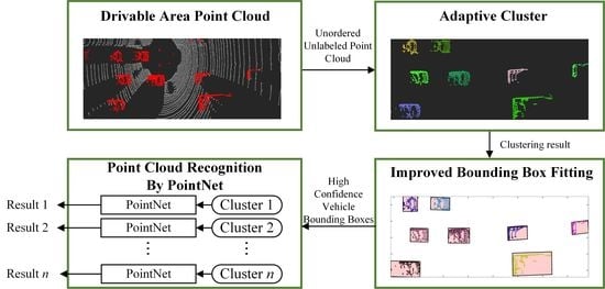
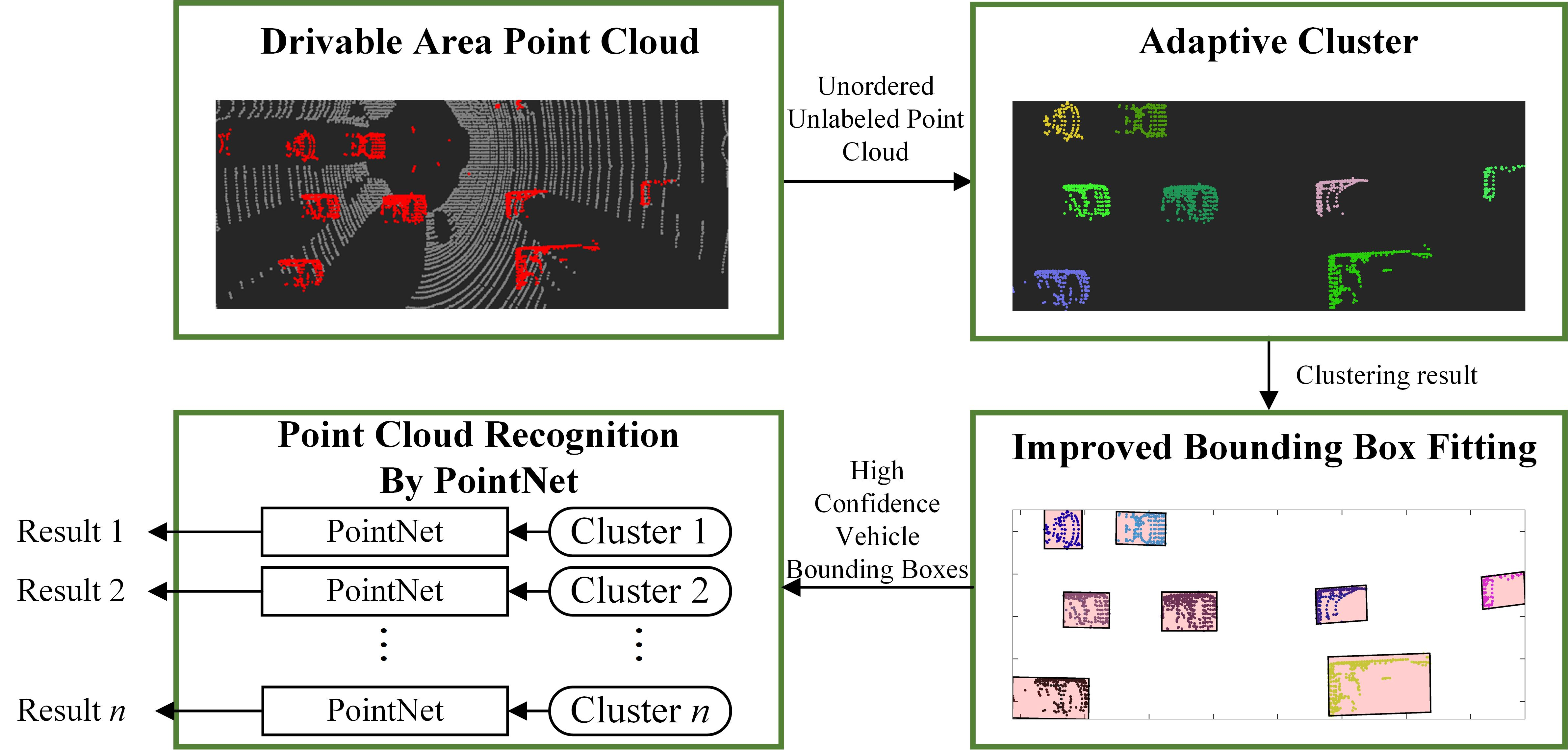
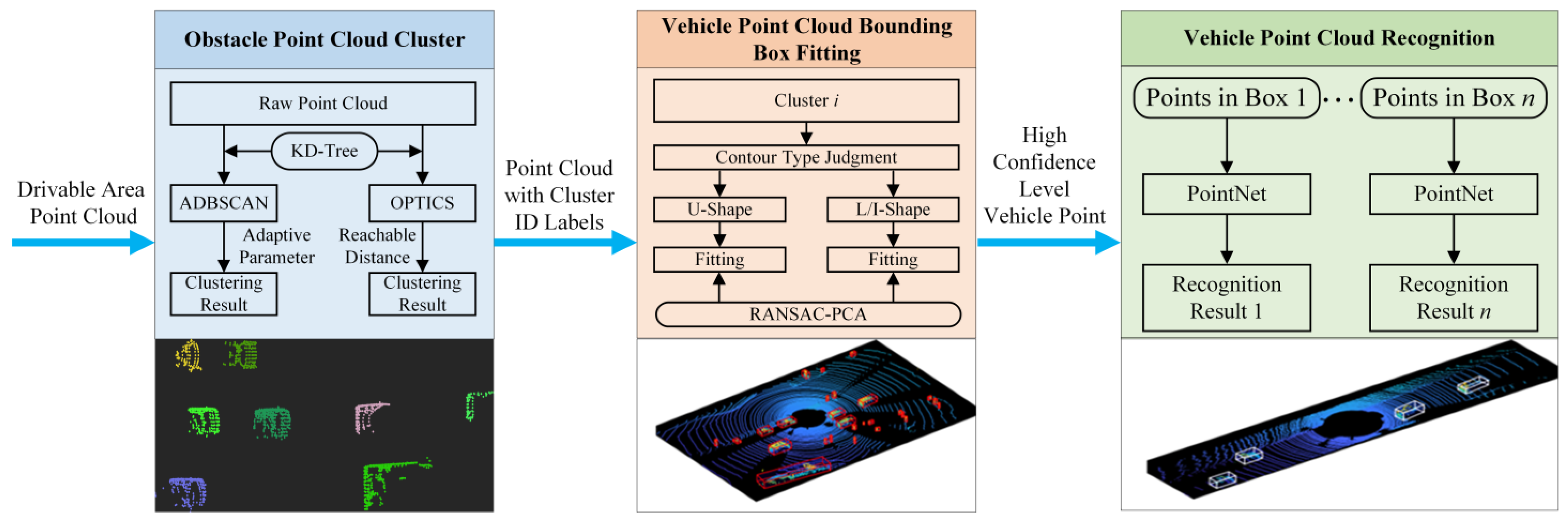
This paper takes point cloud clustering, bounding box fitting and point cloud classification based on deep learning as the technical route and proposes a vehicle detection algorithm based on the combination of clustering and deep learning, the detailed technical route is shown in Figure 1, in which we used the previous work [34] to obtain the drivable area. In simple terms, the ground segmentation algorithm based on the Gaussian process is used to remove the ground point cloud. Experiments with the automatic driving perception platform and the KITTI dataset prove that the proposed clustering algorithm works well, and the bounding box fitting algorithm has high robustness. Moreover, the established technical framework can stably recognize vehicles on the road and achieve a good balance between recognition accuracy and efficiency.
2. Point Cloud Clustering and Vehicle Bounding Box Fitting Algorithm
2.1. ADBSCAN Algorithm for Point Cloud Clustering
In point cloud clustering, the DBSCAN algorithm is a typical density-based spatial clustering algorithm. The DBSCAN algorithm requires that the number of points contained in a certain area in the clustering space is not less than a given threshold minPts. Compared with the most used K-means algorithm, the DBSCAN algorithm does not need to specify the number of categories in the sample in advance, and it can find clusters of any shape and is currently the most used point cloud clustering algorithm in the field of point cloud clustering.
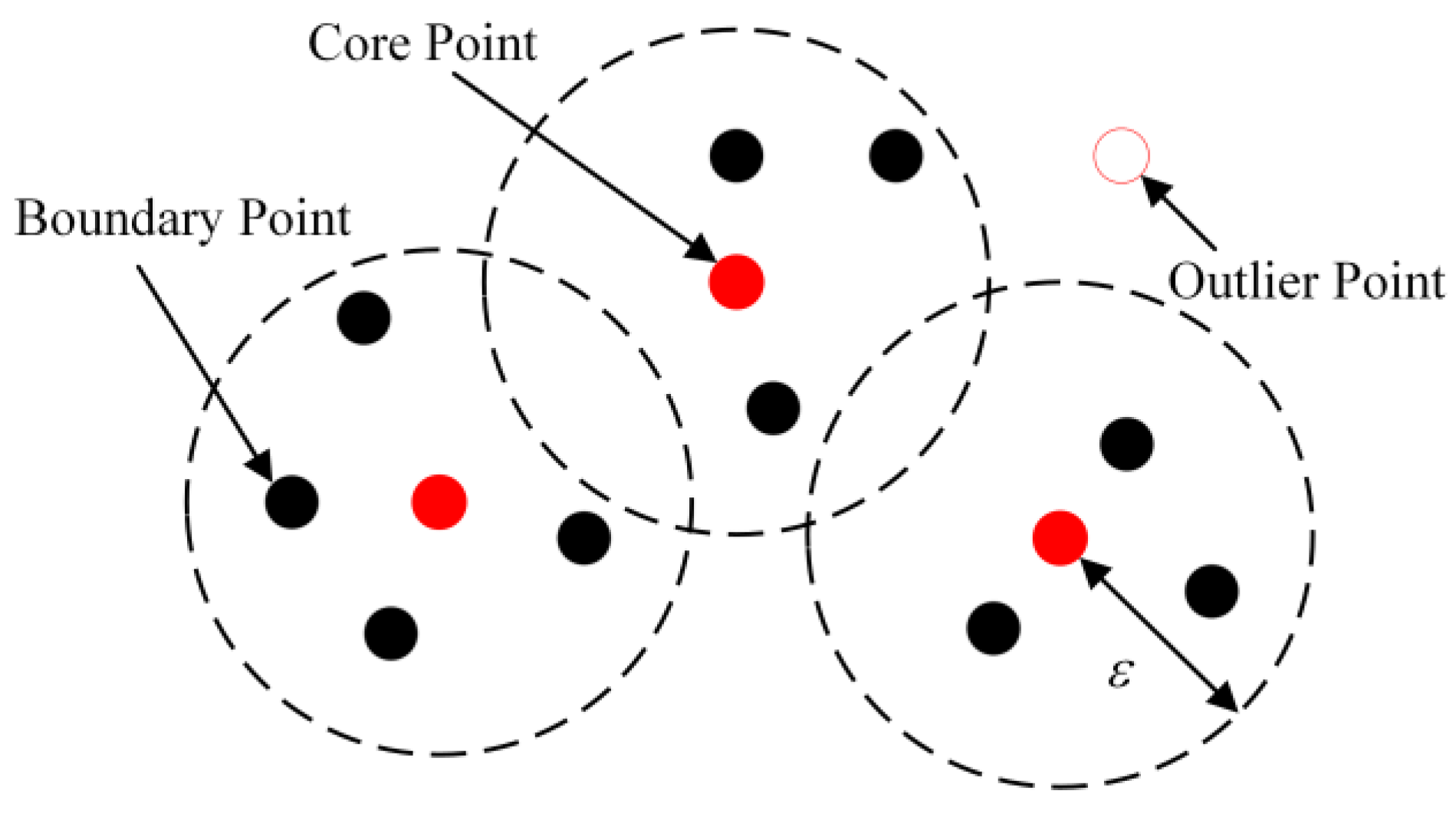
The principle of the DBSCAN clustering algorithm is shown in Figure 2. The algorithm divides the candidate data points into three categories. If the ε neighborhood of sample xi contains at least minPts sample points, that is, Nε (xi) ≥ minPts, the sample point xi is called the core point. If the number of sample points in the ε neighborhood of sample xi is less than minPts but about other core points, the sample point xi is called a boundary point, and finally, the points that are neither core points nor boundary points are recorded as outliers and deleted to obtain the final clustering result.
The traditional DBSCAN algorithm has two parameters that affect the clustering quality, one is the cluster radius and the other is minPts, which is the minimum number of points in a single cluster. Since the distribution of LiDAR scanning points becomes sparse as the distance increases, the clustering radius with a fixed threshold cannot guarantee the clustering quality. At the same time, the DBSCAN algorithm needs to traverse all unvisited points every time to calculate the reachable distance, resulting in the high complexity of the algorithm, and the real-time performance cannot meet the requirements.
Aiming at the above two problems, this paper first improves the clustering radius ε selection method in the DBSCAN algorithm and proposes an adaptive clustering radius based on distance, which enables the algorithm to automatically expand the clustering radius at distant sparse point clouds to obtain more accurate clustering results. Then, in the traversal stage of the DBSCAN algorithm, KD-Tree is used to organize the point cloud data structure to speed up the search.
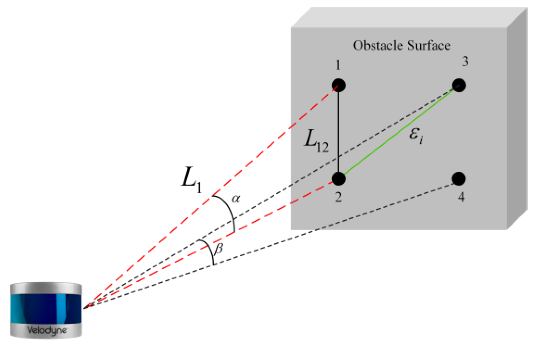
Figure 3 shows the plane scanning model of the LiDAR, where α represents the vertical angle interval of the LiDAR and β represents the horizontal angle interval of the LiDAR. When the LiDAR beam scans the surface of the same obstacle, points 1, 2, 3 and 4 are obtained. According to the arc length formula, the distance L12 between scanning points 1 and 2 is approximately:
At this time, the theoretical minimum clustering radius should be L23. For the robustness of the algorithm, it is appropriately expanded to
In the formula, N is the number of points contained inside when L12 is the clustering radius, η is the expansion coefficient and η = 4 in this chapter. Through the distance adaptation of the cluster radius, the traditional DBSCAN algorithm can in principle adapt to the obstacle point cloud clustering when the point cloud is sparse.
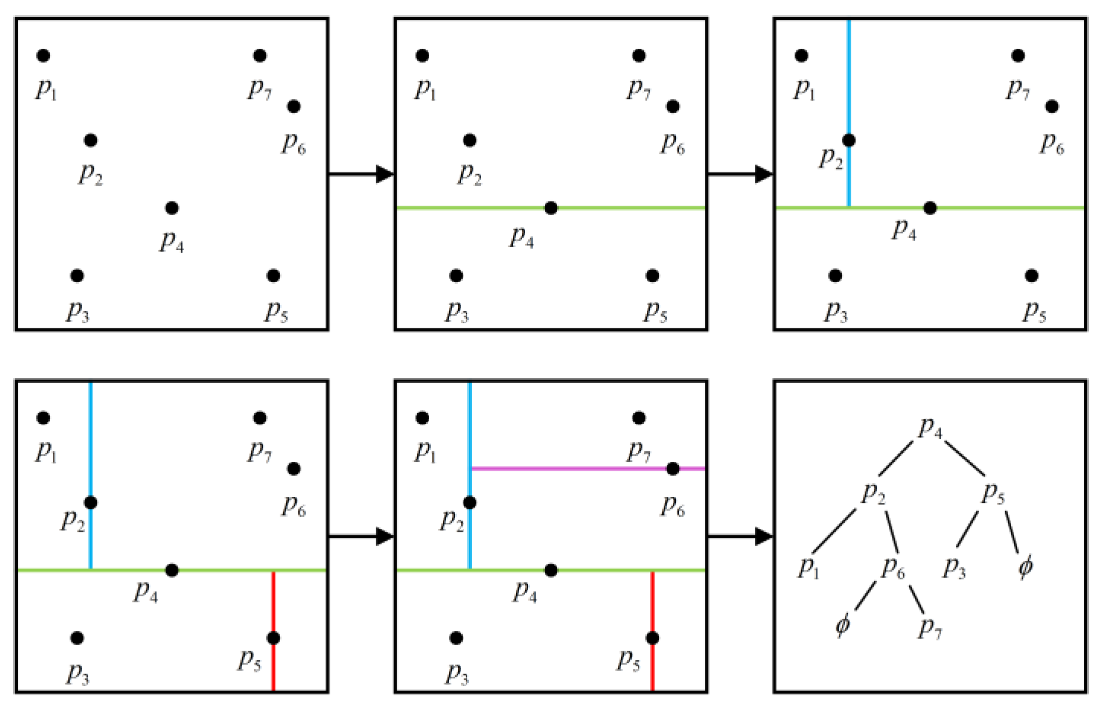
Time-consuming search is also one of the problems faced by the DBSACN algorithm. In order to speed up the search speed of the DBSCAN algorithm, this paper uses KD-Tree to establish a topological relationship for the point cloud. KD-Tree is a tree data structure that stores instance points in k-dimensional space for fast retrieval. It has been widely used in the field of multi-dimensional information search. KD-Tree is essentially a special case of a binary space tree. Each node inside it represents a hyperplane that divides the space, and the data of other multi-dimensional points can be divided according to the value of the node in a certain dimension.
Figure 4 shows the KD-Tree construction process. First, it finds the median of the point set as the hyperplane and divides the initial point set into two parts. In the remaining two parts, it continues to find the median as the hyperplane. Each point set is divided again into two parts until it cannot be divided again. When the KD-Tree is established, the structure of the tree is shown in the last figure in Figure 4. The time complexity of KD-Tree is
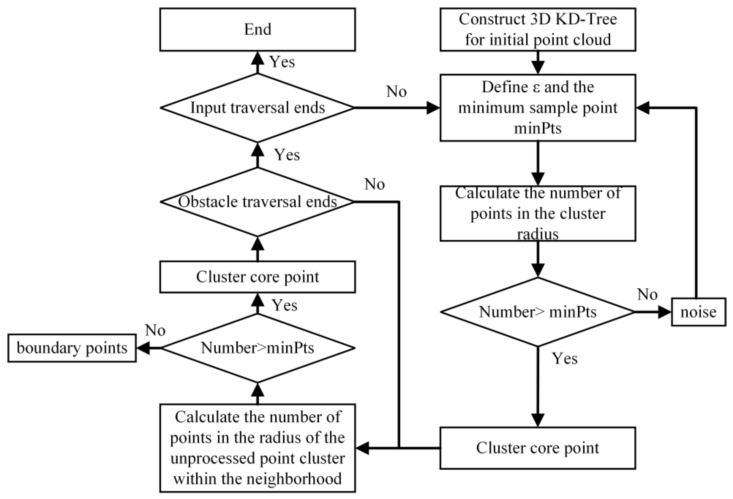
In summary, the process flow of the DBSCAN clustering algorithm based on the size of the adaptive clustering radius proposed in this paper is shown in Figure 5.
2.2. Ordering Points to Identify the Clustering Structure
Ordering Points to identify the clustering structure (OPTICS) algorithm is an improved algorithm for DBSCAN clustering, different from the DBSCAN algorithm that explicitly generates clusters and the output of the OPTICS clustering algorithm is an augmented cluster sorting, which represents the density-based clustering structure of each sample point from which the clustering results based on any cluster radius ε can be obtained, so as to overcome the poor clustering effect caused by the sparse point cloud. As the OPTICS algorithm is rarely used, this paper mainly discusses whether it can be applied to vehicle point cloud clustering, and then gives an evaluation of the algorithm.
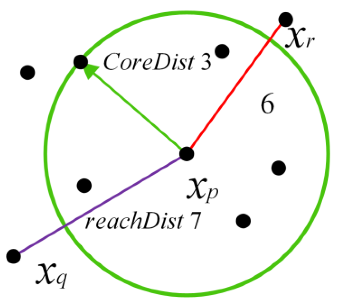
Figure 6 shows the relationship between the parameters. It is generally believed that the clustering radius of the OPTICS algorithm is infinite. The minimum sample constraint minPts is shown in the green circle in the figure. The core distance coreDist(xp) is defined as the distance between the core point xp and the farthest point within the minimum sample constraint range, and the reachable distance reachDist(xq, xp) is defined as the sample The maximum value of the distance between Dist(xq, xp) and coreDist(xp) between point xp and sample point xq. Therefore, the core distance of the sample point xp in Figure 6 is three, and the reachable distance is seven. The pseudo code for clustering using the OPTICS algorithm is shown in Algorithm 1.
| Algorithm 1 OPTICS clustering algorithm |
| Input: X, eps, minPts Output: orderList 01: corepoints = getcoreDist (X, eps, minPts)//Calculate reachable distance 02: coreDist = computecoreDist (X, eps, minPts)//Compute Kernel Distance 03: for unprocessed point p in corepoints 04: Np = getneighbors (p, eps) 05: mark p as processed and output p to the ordered list 06: if Np > minPts 07: Seeds = empty priority queue 08: update (Np, p, Seeds, coreDist)//update sequence 09: for q in Seeds 10: Nq = getneighbors (q, eps)//Number of points to calculate, defaults to all points 11: if Nq > minPts 12: update (Nq, q, Seeds, coreDist)//update sequence 13: return orderList |
After the OPTICS algorithm obtains the augmented cluster sorting, it cannot directly obtain the clustering results. At this time, it is necessary to set the cutoff distance to distinguish different clusters. In the reachable distance image, different depressed regions below the cutoff distance represent different clusters.
2.3. Improved L-Shape Vehicle Bounding Box Fitting
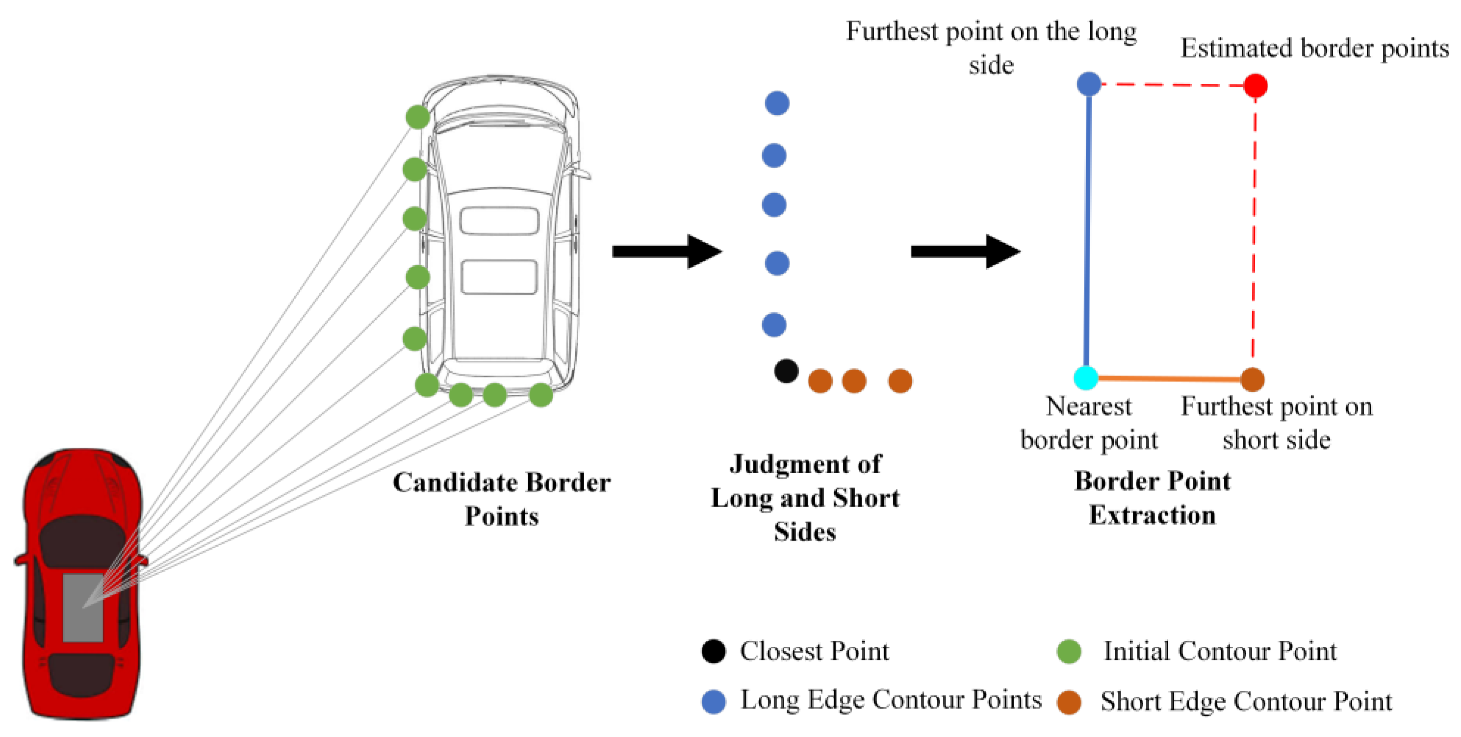
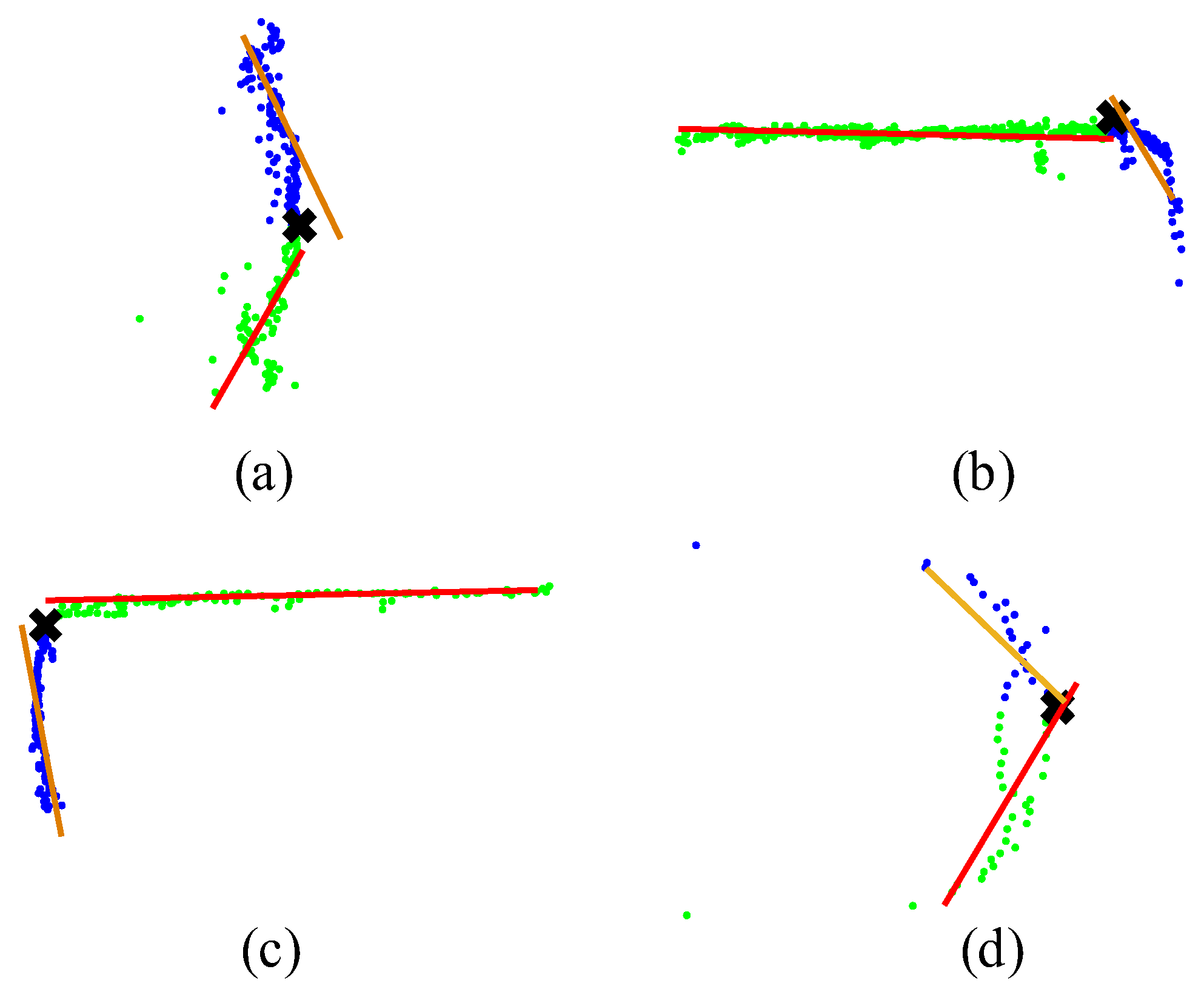
The bounding box fitting algorithm is a method to solve the optimal enclosing space of discrete point sets. Its basic idea is to use a slightly larger bounding box with simple characteristics to approximately replace complex clusters, which is convenient for subsequent identification, tracking and avoidance. The commonly used bounding box fitting algorithm is the minimum area circumscribed rectangle algorithm, but it is not suitable for vehicle bounding box fitting. Considering that the vehicle has an obvious outline, a simple and efficient L-shape algorithm can fit the bounding box of the vehicle. The basic idea of the algorithm is to regard the vehicle contour as an “L” shape, as shown in Figure 7, the algorithm defines the vehicle contour point cloud as the point set with the closest Euclidean distance from the LiDAR at the same angle and defines the closest point as the point where the vehicle contour point is closest to the LiDAR is divided into long and short sides according to the scanning information based on the nearest point. The long side is considered as the left and right sides of the vehicle, and the short side is considered as the rear side of the vehicle. The vehicle point cloud is obtained. After the two sides of the cluster, a straight-line fitting is performed on the two sides to obtain the bounding box. The L-shape algorithm is simple, and the calculation time is low, but there are two strict prerequisites: the first is that the shape of the vehicle contour point cloud needs to meet the L shape or approximate L shape, otherwise, it will appear as shown in the Figure 8a. The case of fitting failure in Figure 8d; the second is that the straight-line fitting algorithm needs to correctly reflect the distribution and orientation of the point cloud, otherwise the long side in Figure 8b and the long side in Figure 8c will appear fitting accuracy is low.
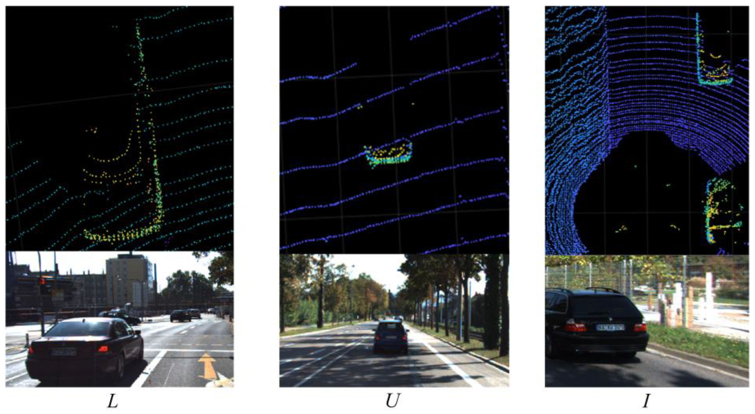
Aiming at the two problems of the traditional L-shape algorithm, an improved vehicle bounding box fitting algorithm is proposed in this paper. The biggest advantage of this algorithm is its high robustness, and it can complete vehicle bounding box fitting in various scenarios. First, it expands the I-shaped and U-shaped vehicle contours based on the L-shaped algorithm. As shown in Figure 9, the I-shaped vehicle contour points are located on the left and right sides of the smart car and are flush with the smart car in the forward direction. The target vehicle and U-shaped vehicle contour points are derived from the target vehicle located directly in front or directly behind the smart car. Through the expansion of the contour type, the algorithm fitting failure caused by the change of the vehicle contour type and caused by the relative attitude is reduced.
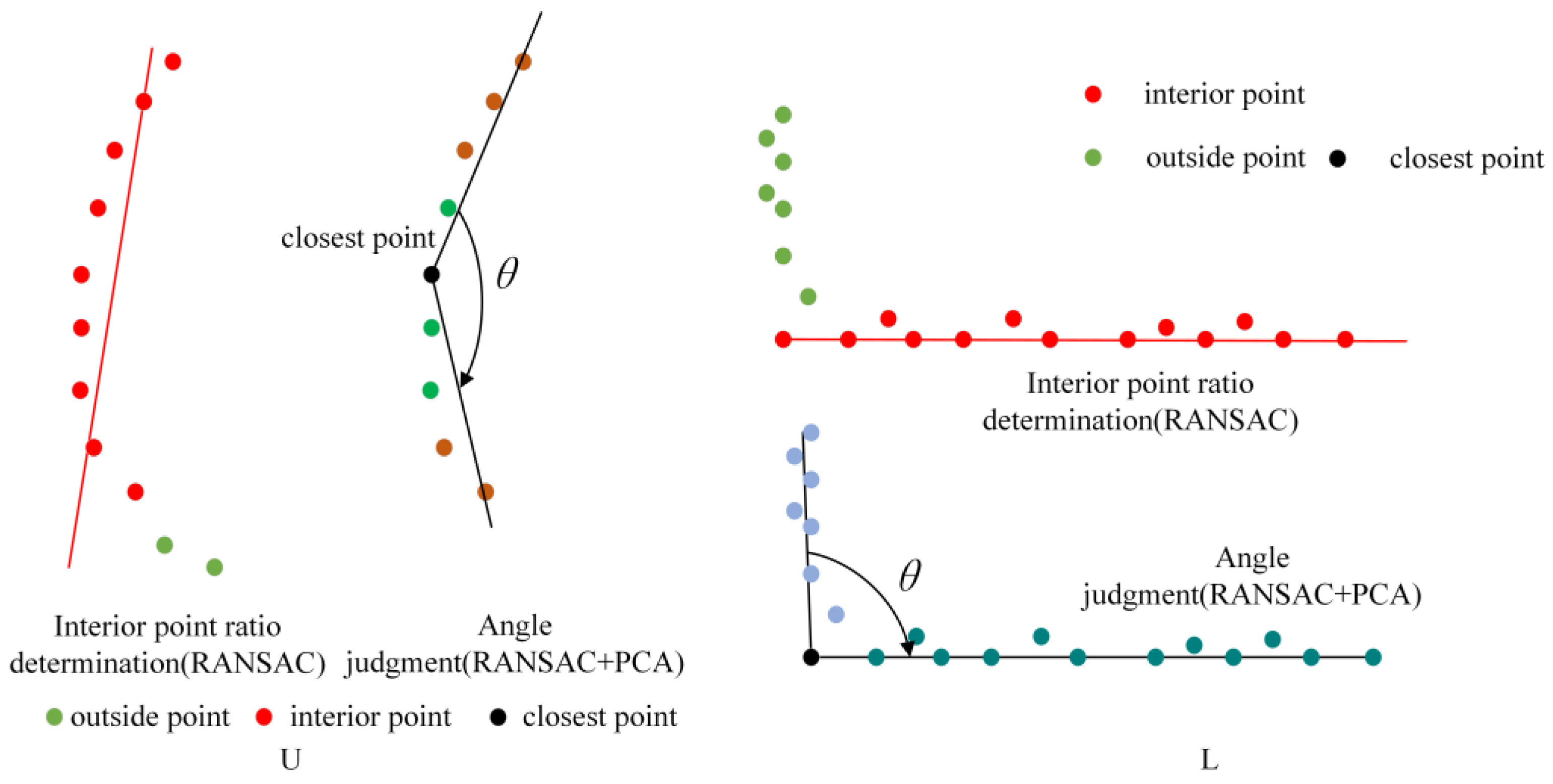
Figure 10 shows the process of judging the vehicle contour point using the angle criterion and interior point rate criterion. The angle criterion takes the nearest point of the initial contour point as the center point, divides the original vehicle contour point into long and short sides and calculates the included angle. The included angle of the L-shaped profile is about 90°, while the U-shaped and I-shaped profiles are greater than 90°. The interior point ratio considers the probability that the contour point distribution is a straight line. When the point cloud distribution is a straight line, the interior point rate of the model iterated by the RANSAC algorithm is high, which can reach more than 90%.
In the angle calculation process, the results obtained by fitting contour points from commonly used straight line fitting algorithms such as the RANSAC algorithm and the least squares fitting algorithm cannot fully reflect the distribution characteristics of the vehicle’s contour points, which leads to subsequent angle judgments. Thus, this paper introduces the Principal Component Analysis (PCA) algorithm and combines it with the RANSAC algorithm to ensure the robustness of the calculation of the contour point direction.
The PCA algorithm is a statistical method for dimensionality reduction. It uses an orthogonal transformation to recombine the original variables into a new set of unrelated comprehensive variables and then extracts a few fewer variables from them according to actual needs to respond as much as possible. The original variable information. For the obstacle contour point set P = {p1, …, pi}, the covariance matrix M is constructed as
where
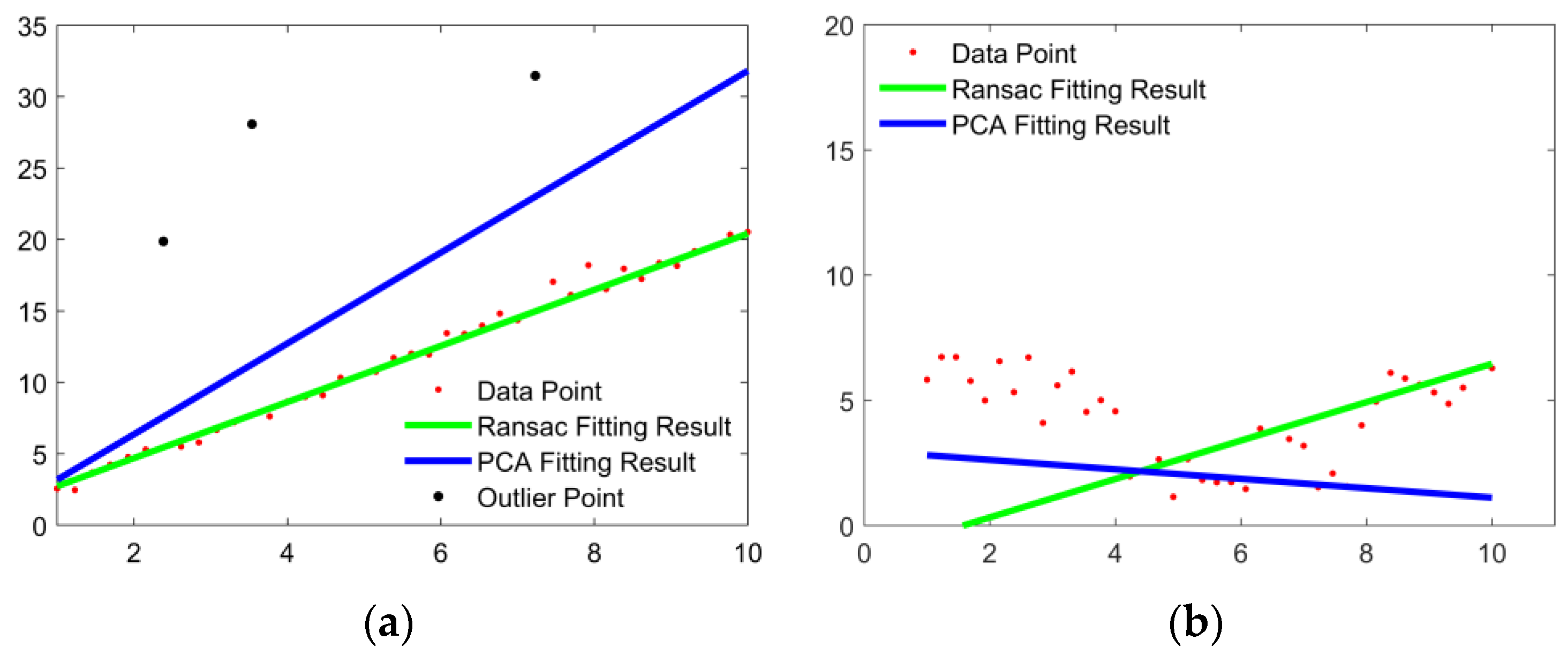
In the formula, λ = (λ0, λ1, λ2) is the eigenvalue, and V = (V0, V1, V2) is the corresponding eigenvector. The larger the eigenvalue of the eigenvector, the greater the change of the sample set in this direction. Since most of the contour points are linearly distributed, the eigenvector at this time can be oriented to the point cloud of the entire contour point. However, the PCA algorithm does not have the ability of the RANSAC algorithm to reject outliers. When there are some outliers in the data, the PCA algorithm cannot filter them out. As shown in Figure 11, when there are outliers in the data, since the PCA algorithm reflects the distribution characteristics of all point clouds, the black outliers are also included and the fitting result is quite different from the real point cloud distribution. The RANSAC algorithm does not consider all points, so the black outlier points are directly rejected during the fitting process, and the robustness is high. Figure 11b shows the shortcomings of the RANSAC algorithm. When the point cloud distribution has a certain curvature, such as the rear bumper of the target vehicle, the rear trunk, etc.; the fitting results of the RANSAC algorithm will have serious deviations and cannot be applied to this class.
Therefore, this paper proposes the RANSAC-PCA algorithm to improve the stability of the straight-line fitting process. In the straight-line fitting stage, the initial point is first screened using the RANSAC algorithm, and then the interior points obtained by the RANSAC algorithm are recorded as sampling points, and finally the PCA algorithm is used to fit the sampling point set. Among them, the RANSAC algorithm divides all points into outer points and inner points and then the PCA algorithm estimates the orientation of the inner points, and uses the estimated result to represent the orientation of the point cloud, that is, the outline of the bounding box of the vehicle, effectively avoiding the interference of abnormal points while ensuring towards the robustness of the fitting results.
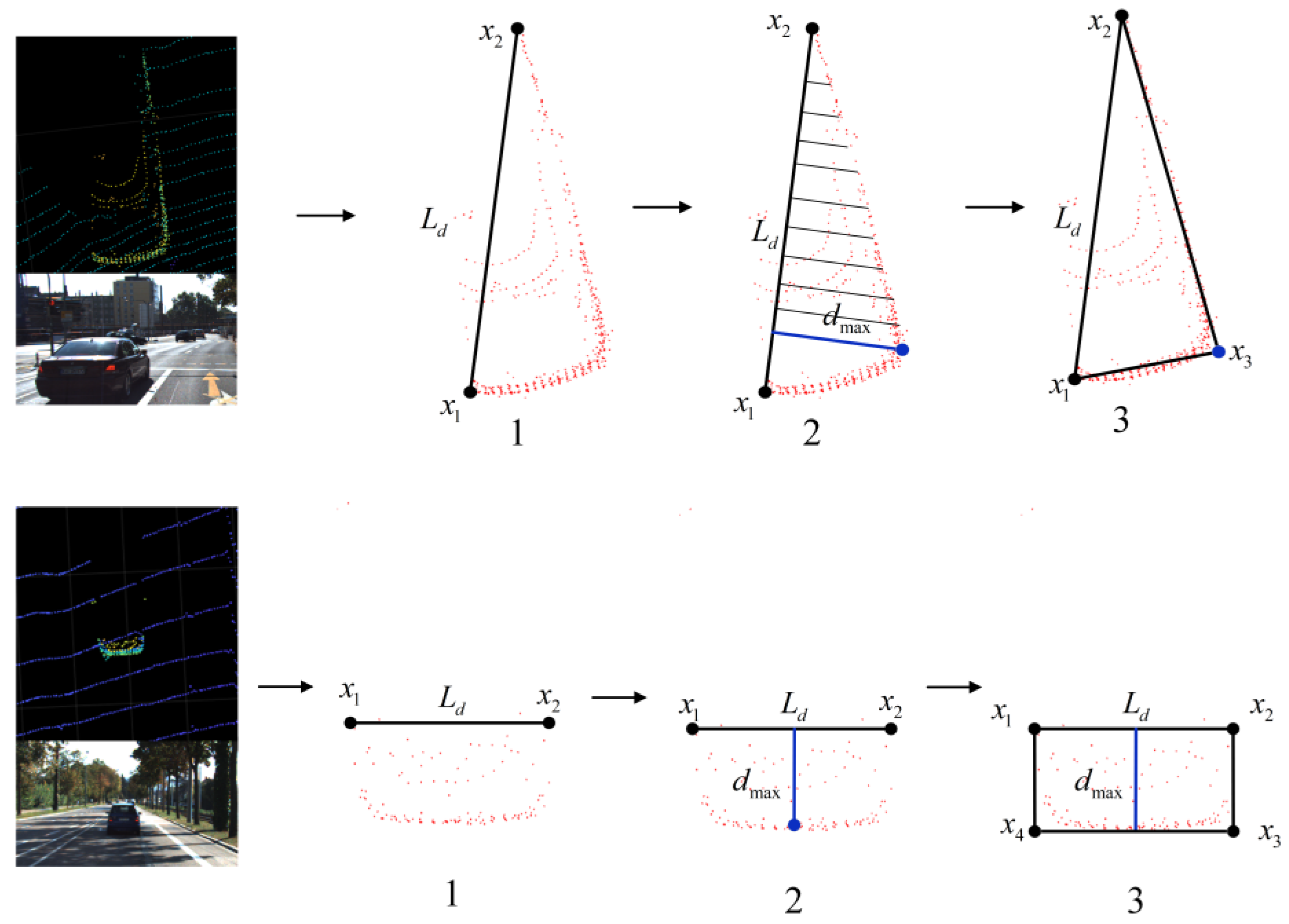
In summary, the process flow of the bounding box fitting algorithm proposed in this paper is shown in Figure 12. For the L-shaped contour, first, find the nearest point and the farthest point, and then find the point farthest from the straight line formed by the two points in the contour point set, use it as the corner point and finally obtain it according to steps 2 and 3 in Figure 12 to the bounding box. For the U-shaped contour, find the leftmost and rightmost points, and then similarly find the point farthest from the straight line connecting the two points, and finally obtain the bounding box according to steps 2 and 3 in Figure 12.
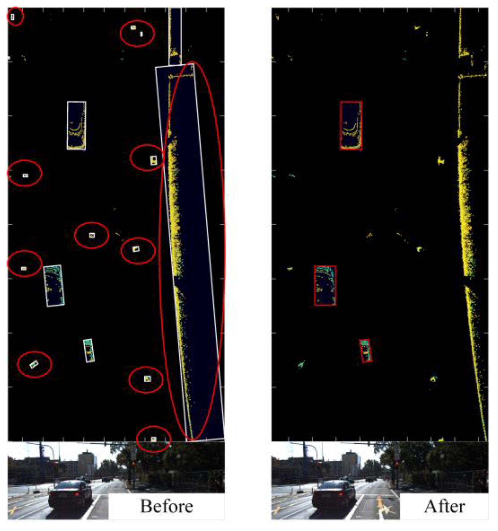
Before the clustering results are sent to the point cloud classification network for recognition, the point cloud clusters that obviously do not have vehicle characteristics are excluded in advance from the bounding box fitting results, which can effectively reduce the time-consuming recognition. In addition to the basic characteristics such as length, width and height, the following indicators are also defined, as shown in Table 1. It should be noted that the starting point of this link is not to find clusters with vehicle characteristics but to delete obvious non-vehicle clusters such as rods and thin walls. Figure 13 shows the number of obstacles after screening. It can be found that in the screening, other obstacles such as walls, bushes, trees and utility poles can be quickly and effectively eliminated.
After that, the point cloud inside the vehicle bounding box, which is considered to have high confidence, will then be fed into the point cloud classification neural network for further semantic recognition.
3. Vehicle Point Cloud Recognition with PointNet
3.1. PointNet Point Cloud Classification Network
The traditional vehicle point cloud recognition method relies on machine learning. After extracting the global features such as linearity, flatness, volume and curvature change value of the point cloud, use a trained SVM, random forest or Adaboost to classify and identify it. However, the training of classifiers is very time-consuming. In addition, the input object of the classifier is manually extracted point cloud global features, which leads to the classification result largely depending on whether the designed features can accurately describe the vehicle target. Therefore, considering the amount of training, algorithm transferability and recognition accuracy, this section introduces the PointNet point cloud classification network and uses the result of the bounding box fitting algorithm as input to identify the point cloud in the high confidence vehicle bounding box.
Deep learning has achieved a lot of results in image recognition, intelligent manufacturing, data mining and other fields. The basic idea is to combine certain features of the input data to obtain more diverse features, and then to input data is differentiated and identified. After years of development, a series of algorithms represented by neural networks have emerged such as Convolutional Neutral Networks (CNN), Generative Adversarial Networks (GAN), Long-Short Term Memory Network (LSTM), etc.
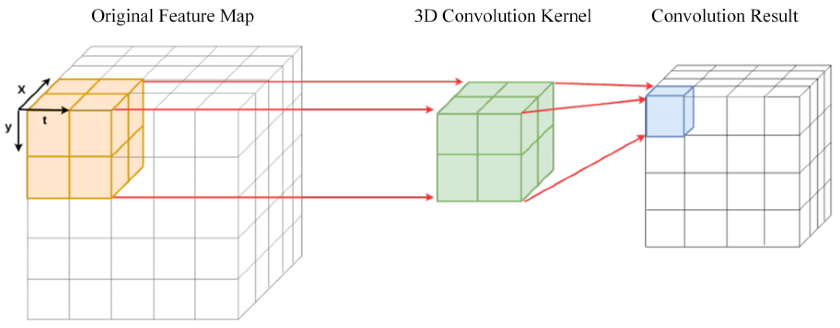
The principle of three-dimensional convolution is like that of two-dimensional convolution. The difference is that there are more depth channels. The information that can be represented by this channel includes the number of video frames, three-dimensional graphic slices or distance information of point clouds. Three-dimensional convolution is at the height of the input data. Convolution operations are performed in the directions, width and depth, and finally, three-dimensional convolution information is obtained. The principle is shown in Figure 14.
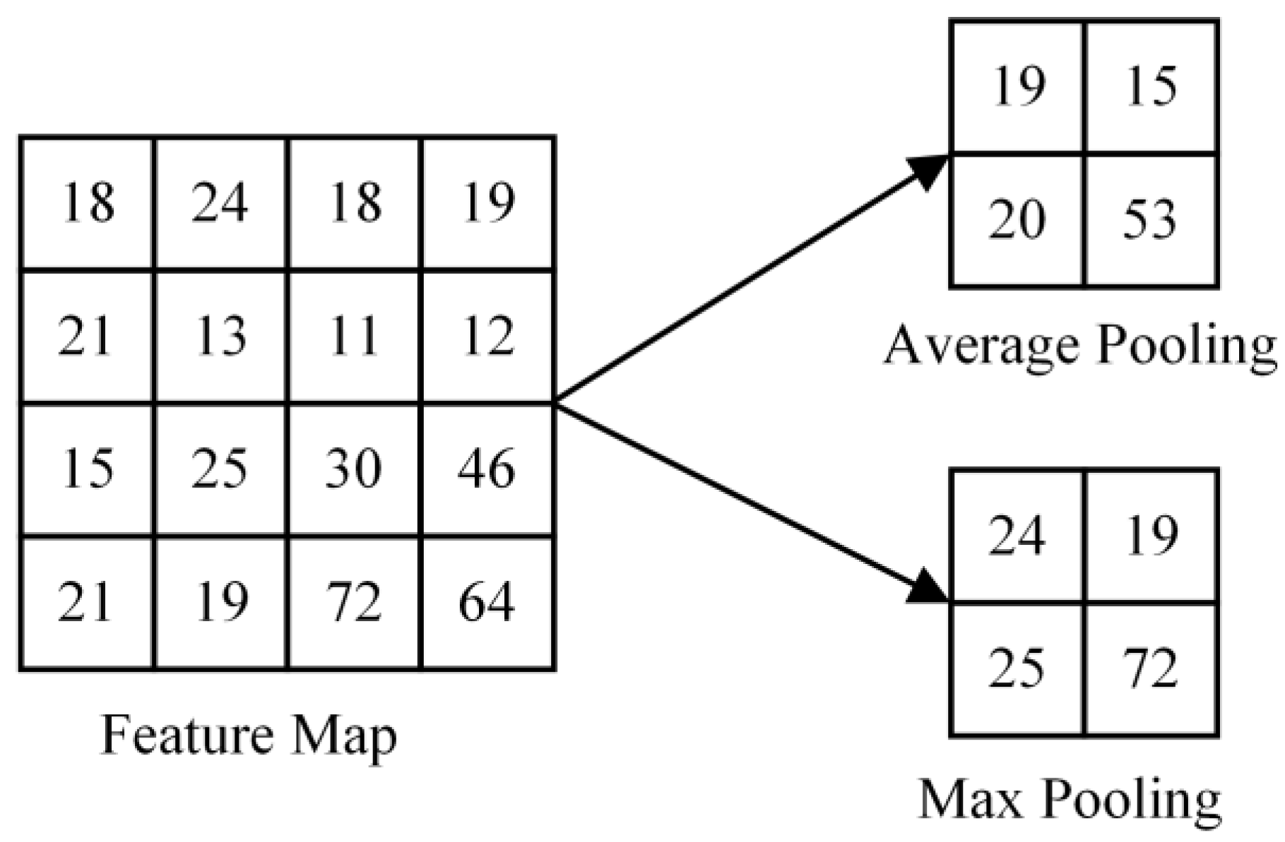
The purpose of the pooling layer is to reduce the dimension of the feature map and retain a large amount of important information. There are two general pooling methods: max pooling and average pooling. Figure 15 shows the feature map and the results obtained after operating with maximum pooling and average pooling, respectively. Maximum pooling first selects a fixed-size window, regards the largest element in the window as a feature value and then completes feature value extraction through a sliding window. The average pooling method is the same as the maximum pooling; the difference is that the selected feature value is the average value in the window.
The fully connected layer is at the end of the convolutional neural network. After the previous convolution has learned enough features, the high-dimensional features are reshaped into a one-dimensional vector inside the fully connected layer, and the classification results are output. The main function of the classifier is to learn the potential classification rules from the existing data categories and it can complete the classification when the location data is input. Commonly used classifiers such as support vector machines and logistic regression are mainly used to solve binary classification problems and it is difficult to face multi-classification problems. SoftMax has been widely used in the field of multi-classification and the effect is remarkable. The principle is to map the output category of the network to the (0, 1) interval to indicate the probability that the target belongs to a certain category so that no matter how many types of labels there are. SoftMax can output the probability corresponding to each label and take the one with the highest probability Labeling completes the classification task.
Since the convolutional architecture requires a highly regular input data format in order to share weights or perform kernel optimization, and point clouds and grids are in unusual formats, most methods first convert point cloud data into regular 3D voxel grid or collection of images before feeding it into a deep network architecture for recognition. Obviously, such processing will change some of the original features of the point cloud. Charles R. Q of Stanford University proposed a classification and segmentation method based on point cloud global features—PointNet in 2017 [7].
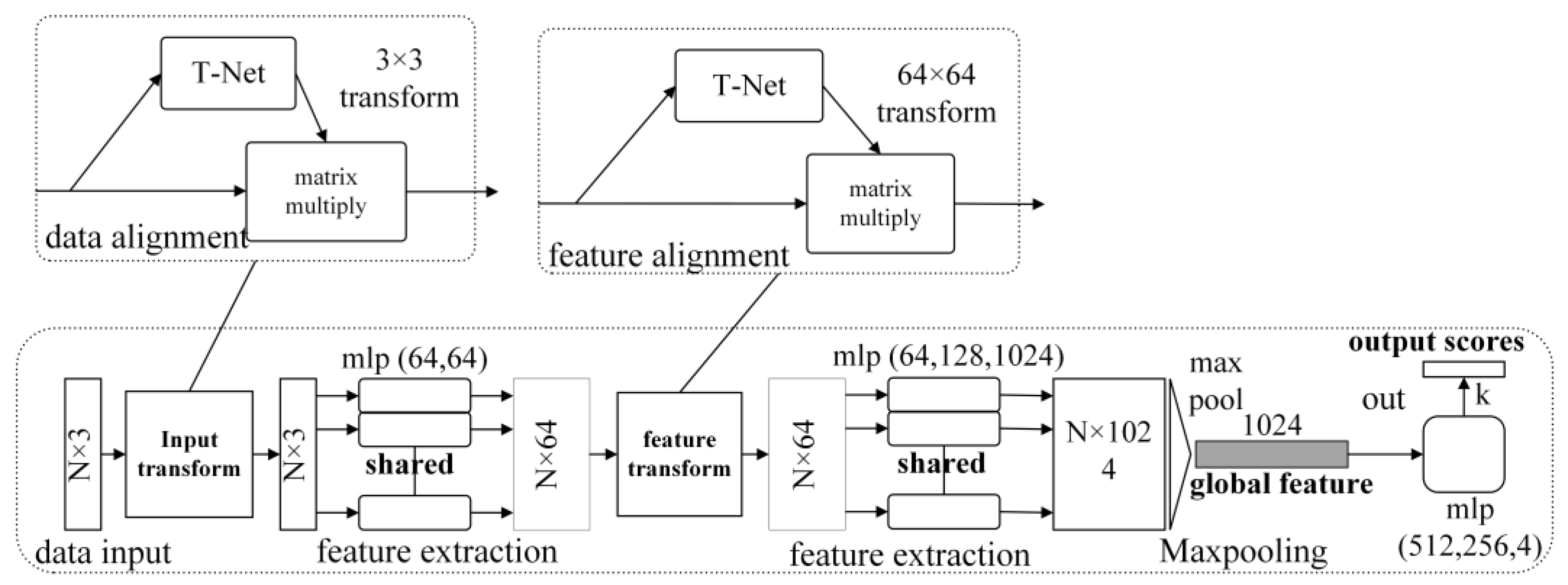
PointNet is a new type of deep learning model for processing point cloud data, which can be used for various cognitive tasks of point cloud data such as classification, semantic segmentation and target recognition. Its network structure is shown in Figure 16. PointNet directly takes point cloud data as input, and it multiplies with a transformation matrix learned by T-Net to ensure the invariance of the model to a specific space transformation, and then uses multiple weight-sharing multi-layer perceptrons to extract features from the point cloud and obtain (N, 1024) the size tensor, after convolution, obtain 1024-dimensional vector features for each point, then use the transformation matrix learned by T-Net again for feature alignment and finally utilize the maximum pooling method to obtain the global features of the point cloud to complete the classification or split tasks. The core modules of the PointNet network includes the T-Net alignment module, multi-layer perceptron, maximum pooling and full connection.
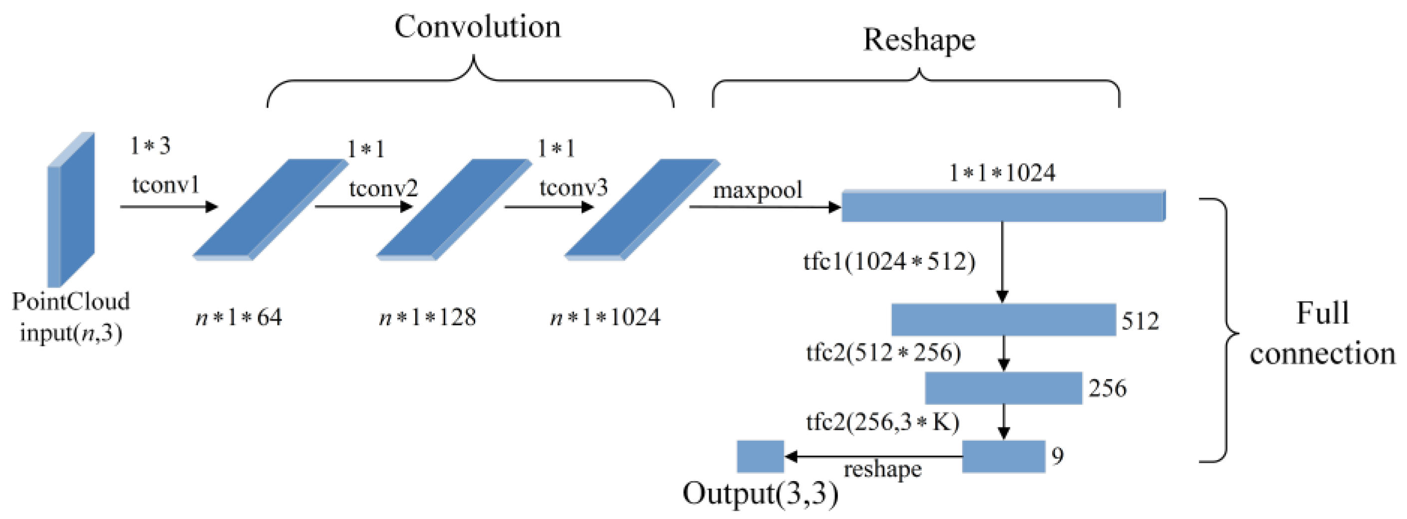
The two T-Net alignment module structures used in the PointNet network structure are shown in Figure 17. Since the order of points in the point cloud does not affect the spatial structure of the point cloud itself, different input orders will affect feature extraction, that is, if the order of the input point cloud is different, the MLP layer will extract different high-dimensional features. Therefore, the input point cloud must be processed with the T-Net module to ensure the input invariance of the point cloud. The T-Net module consists of three parts. The first part consists of three layers of shared MLP for feature extraction; the second part is a symmetric function for aggregating global information; the third part is a two-layer fully connected hidden layer plus a linear layer for predicting affine transformations matrix. In addition, the first T-Net module in PointNet is used to align the input point cloud to ensure the invariance of the spatial rigid body after the point cloud data is fed into the network. The second T-Net module is used to align the point cloud features extracted by the multi-layer perceptron. The T-Net module adds a regularization term to the network training loss, constraining the matrix to be nearly orthogonal:
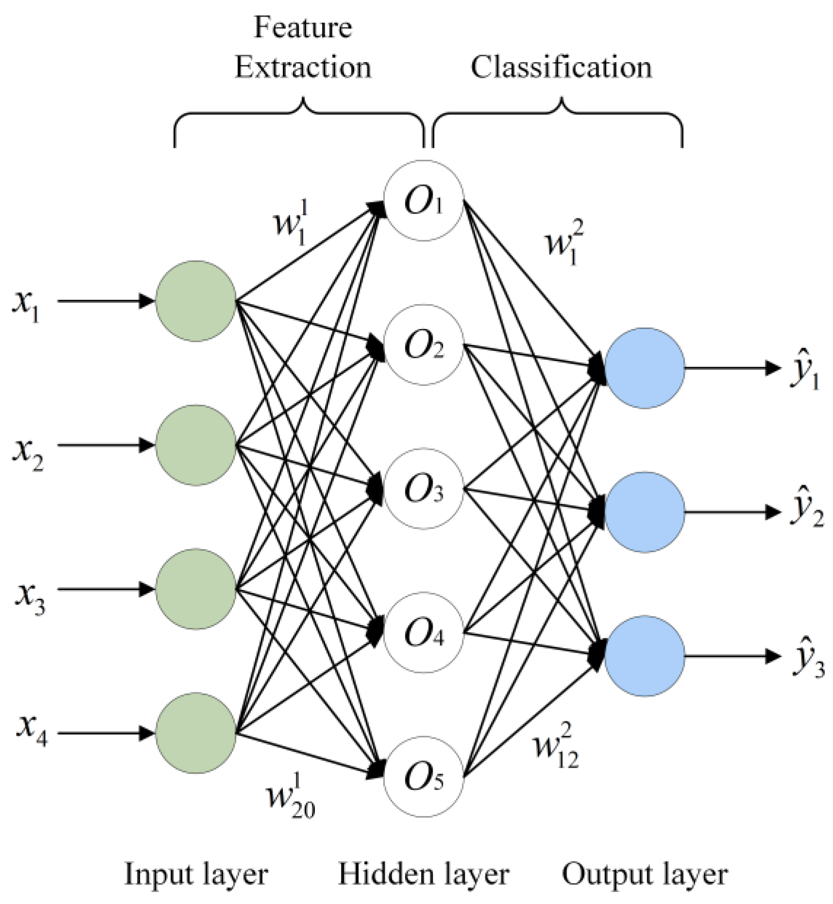
Multi-layer perceptron: multi-layer perceptron consists of an input layer, multiple hidden layers and an output layer. The layers are fully connected. Each neuron is equipped with a nonlinear activation function. Its structure diagram is shown in Figure 18, and the calculation process is represented by Formulas (8)–(10), where W represents the parameter matrix, g is the activation function of the hidden layer and G is the global feature.
Max pooling (maxpooling): PointNet uses the maximum symmetric function to approximate the function defined by any point set, avoiding the influence of the data order on the result to solve the disorder problem of point cloud:
In the formula, f (.) represents the point cloud global feature extraction function, and h (.) represents the point feature extraction function.
Full connection: PointNet finally extracts the features of the points through the multi-layer shared weight MLP and outputs the predicted category of each point after inputting the connected 64-dimensional local features and 1024-dimensional global features into the classifier. Since PointNet maximizes all points into a global feature, the connection between local points and points is not captured by the network, and the local features of the point cloud are lost. When the scene becomes complex, the accuracy of the PointNet network drops significantly, not suitable for segmentation tasks.
In summary, this paper builds a PointNet network for the final point cloud recognition. Since the pre-processing part has obtained a high-confidence vehicle bounding box, this method not only has the robustness of the traditional method but also can obtain the semantics of the vehicle point cloud. Information can achieve a better balance between recognition accuracy and time-consuming.
3.2. PointNet Training Process
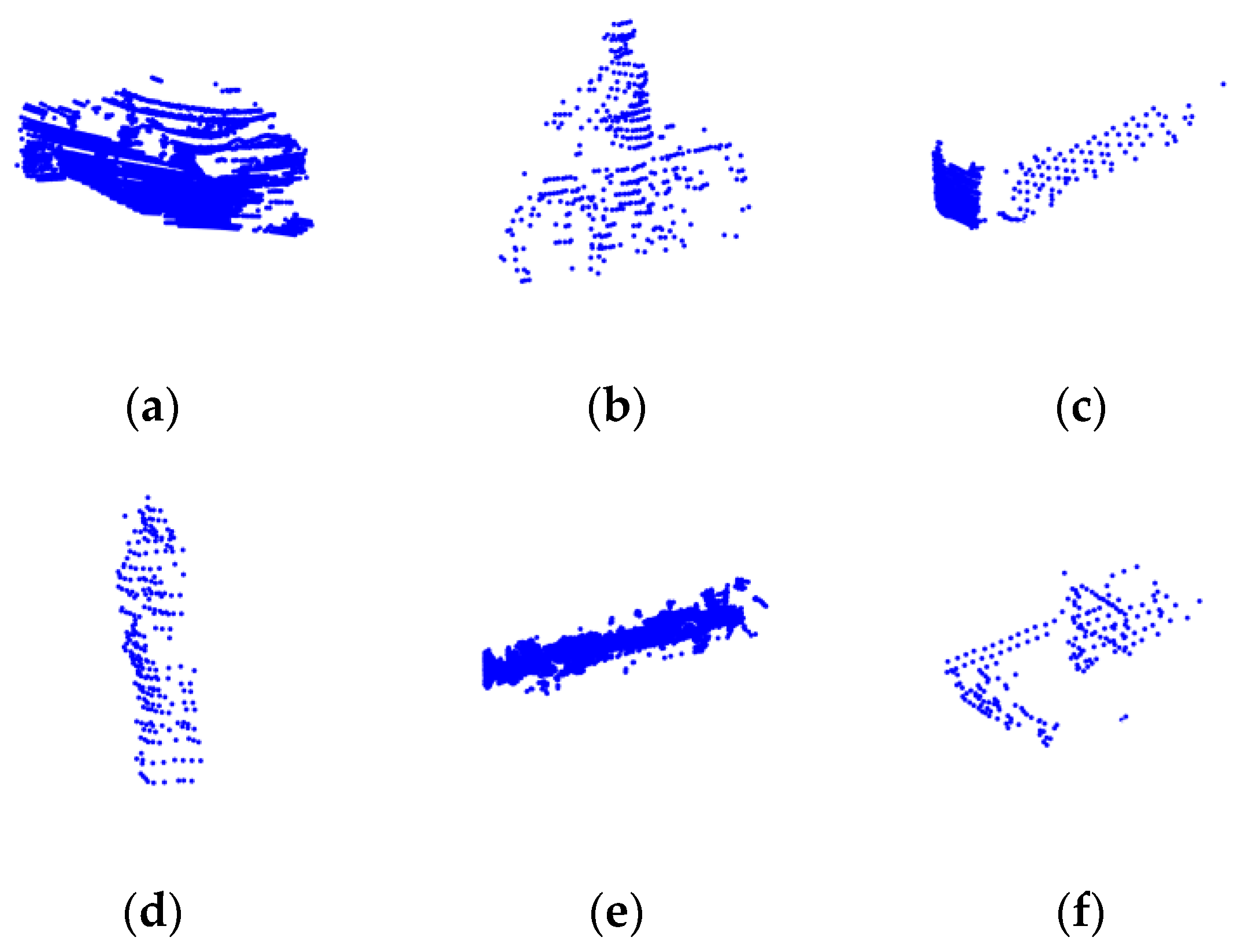
The training data in this paper comes from the KITTI Object 3D dataset. Since this dataset does not provide classification data, we extract 18,566 original objects through the conversion relationship between the image and LiDAR system, as well as the labels and bounding boxes provided in the Training dataset. Obstacle data, a total of six categories, as shown in Figure 19, including “Car”, “Pedestrian”, “Cyclist”, “Van”, “Misc”, “Truck”. We convert “Car”, “Van”, and “Truck” into “Car”, keep “Pedestrian” and “Cyclist” and classify the rest as “Other”. In the end, 10,341 “Car” samples, 4767 “Pedestrian” samples, 1863 “Other” samples and 1595 “Cyclist” samples are obtained.
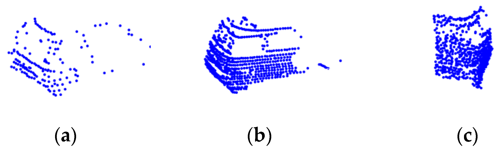
Since most of the KITTI datasets are road scenes, the proportion of samples belonging to the category “Car” is relatively high. If the proportion of single-class samples is too large, the generalization ability of the network model will be poor. For classes with a small number of samples, it will be expanded by random deletion, rotation around the Z axis and Gaussian random noise after copying. Furthermore, since the number of points per class varies a lot within and between classes, the input requires samples to maintain the same number of points, usually 1024. Therefore, for samples with more than 1024 points, use downsampling technology to reduce the number of points, and for samples with less than 1024 points, use zero padding to expand it, as shown in Figure 20. The sample size and proportion after data enhancement are shown in Table 2.
The cross-entropy loss function adopted by the point cloud classification network is
In the formula, M represents the number of preset categories in the label, yic is a sign function and takes 1 if the prediction result is consistent with the label, otherwise it takes 0 and pic represents the predicted value of the probability that sample i belongs to category c. The Adam optimizer is used for optimization, the initial learning rate is set to 1 × 10⁻³, the maximum number of iterations epoch is set to 100 and the batch size is set to 256.
4. Experiment Results and Analysis
In the experimental stage of this paper, the LiDAR point cloud data in the KITTI dataset is mainly used for algorithm verification. The KITTI dataset is a dataset widely used in the fields of computer vision and autonomous driving, jointly launched by the Karlsruhe Institute of Technology and the Technical University of Munich, Germany. This dataset contains various data such as RGB images, LiDAR data, camera calibration information, vehicle trajectories and road maps in various scenarios.
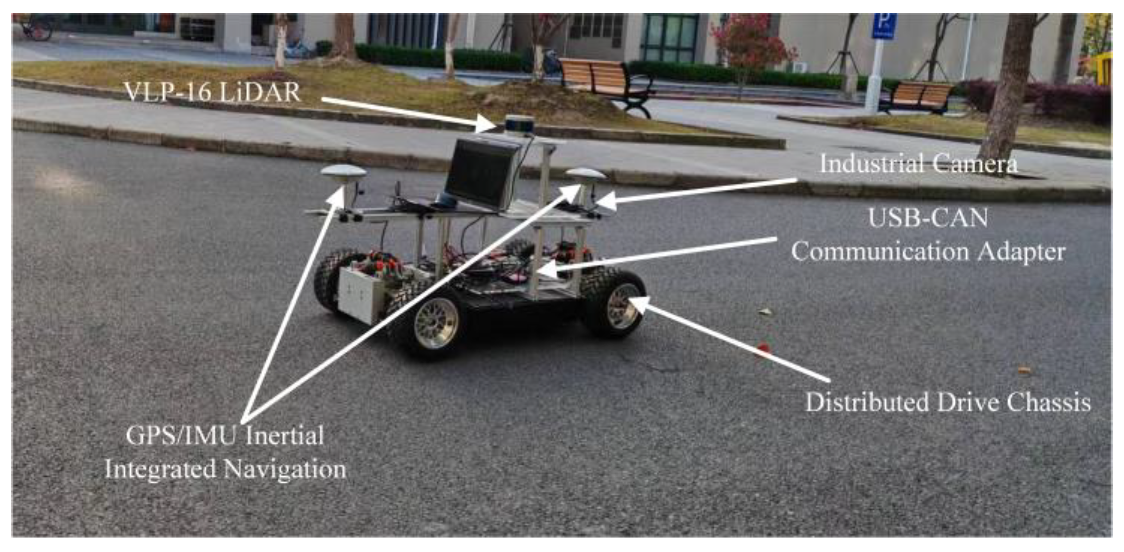
In addition to the KITTI dataset, this paper also collects structured road point cloud data in the campus environment through the autonomous driving perception platform built in our laboratory (Intelligent Electric Vehicle Laboratory, iEVL, Shanghai, China) to verify the performance of the algorithm in some specific scenarios. As shown in Figure 21, the platform is driven by a distributed drive chassis equipped with hub motors, equipped with a Velodyne VLP-16 LiDAR made by Velodyne, a Mako-502C industrial camera made by Allied Vision, Nuvo-6108GC industrial computer and a GPS module with integrated IMU. Able to complete point cloud and image data collection and experiments for motion planning algorithm verification. Among them, the number of lidar wire harnesses is 16, the accuracy is ±3 cm, the working frequency is 10 HZ and the maximum scanning distance is 100 m.
Since our platform cannot be compared with the platform that is installed on the self-driving vehicle, our test session mainly focuses on verifying the effectiveness of the algorithm and making a time-consuming relative comparison.
4.1. Validation of Clustering Algorithms
Firstly, the effectiveness of the clustering algorithm proposed in this paper is verified. A comparison between the ADBSCAN algorithm and the OPTICS algorithm is provided. The clustering radius of the TDBSCAN algorithm is set to 0.8 m, the cut-off distance of the OPTICS algorithm is set to 1.2 m and the minimum number of sample points minPts for the three types of algorithms is all set to 10.
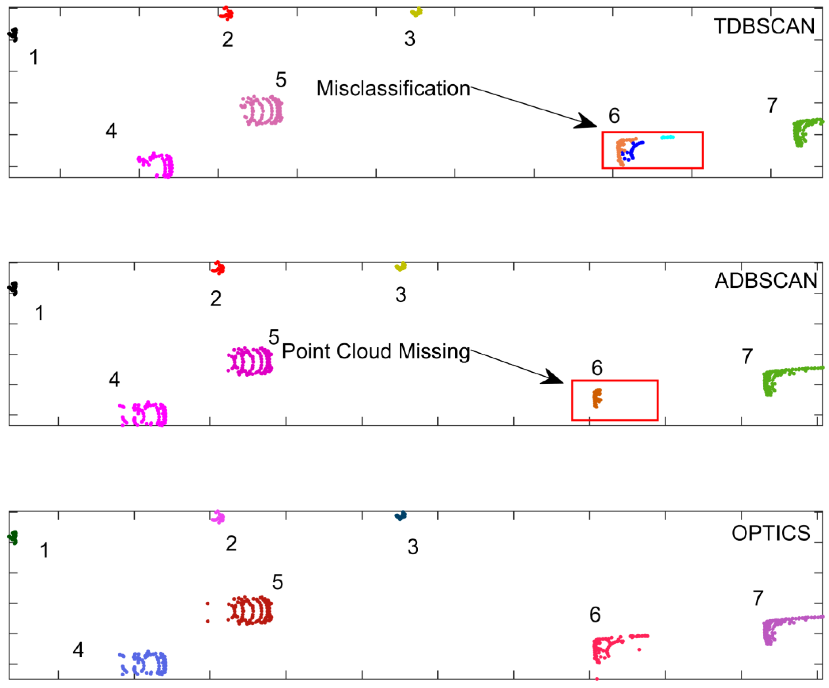
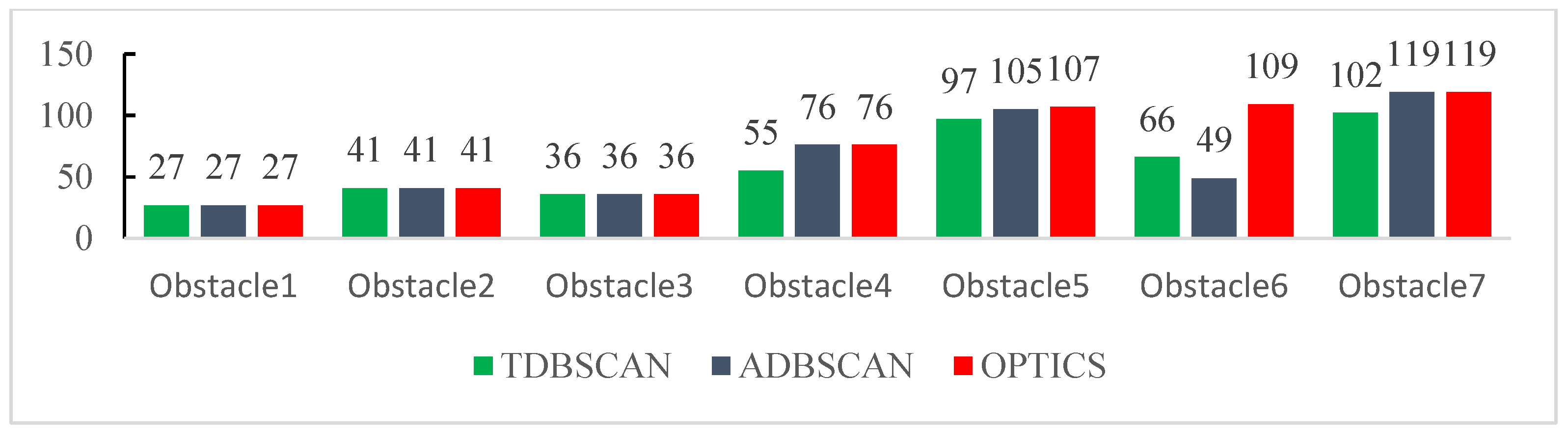
Figure 22 shows the clustering effect of the three types of algorithms in the KITTI dataset 2011_09_26_0013, and the statistics of the clustering results for each obstacle are shown in Figure 23. For obstacles with small sizes and simple shapes, there is no difference in the clustering effect of the three types of algorithms. When the clustering targets are vehicles 4, 5, 6 and 7, the clustering effect of the algorithm is different. Among them, the clustering result for obstacle 6 is the most obvious. TDBSCAN directly divides obstacle 6 into three categories, the ADBSCAN algorithm has no wrong clustering but lost about 55% of the point cloud data.
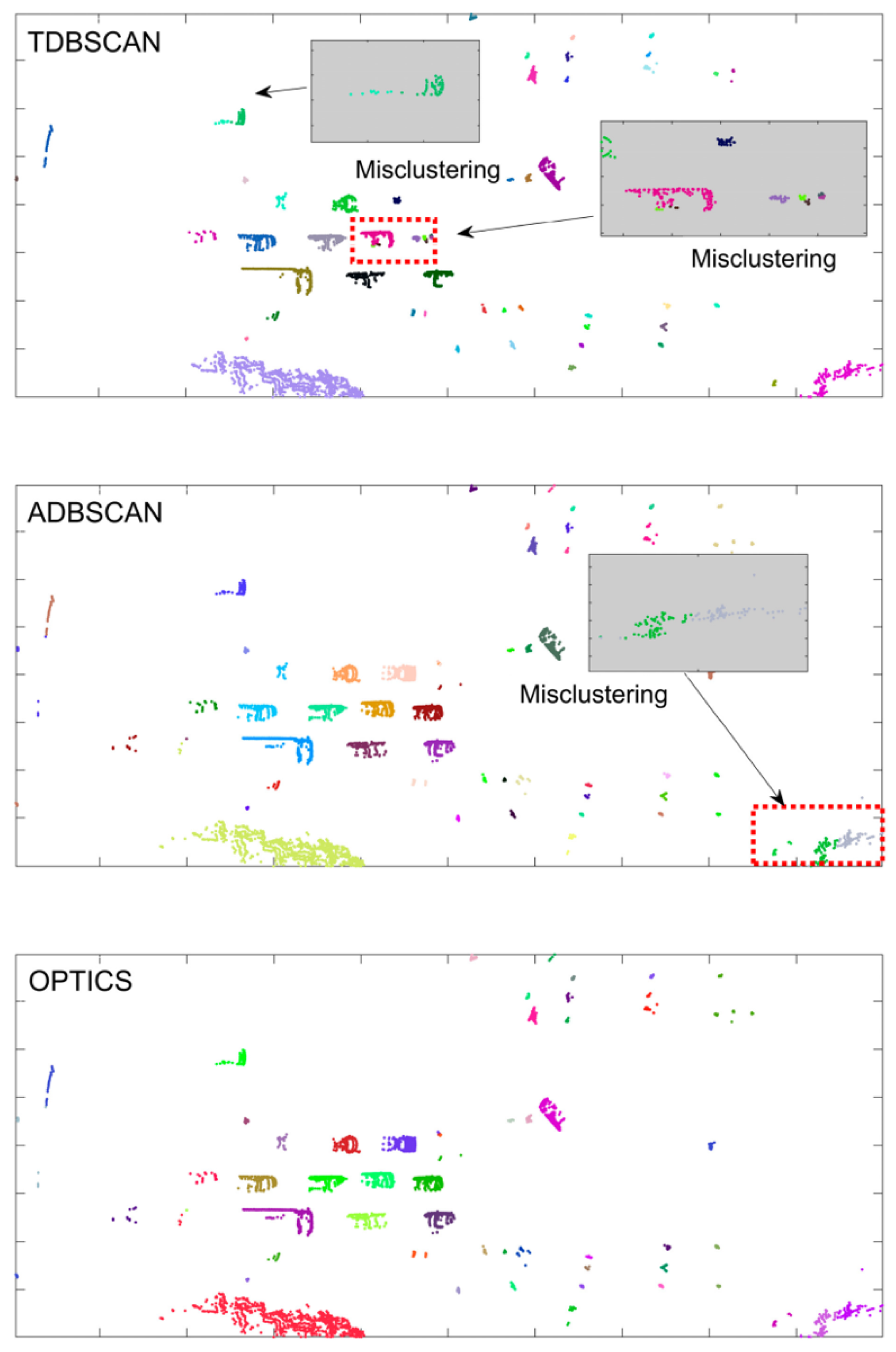
Figure 24 qualitatively shows the clustering results of all obstacles in dataset 0018. The clustering effect of the TDBSCAN algorithm on vehicles is poor and the same vehicle is clustered into two results; the ADBSCAN algorithm can cluster the vehicles well, but the clustering in the distance appears mistake. The OPTICS algorithm is obviously ahead of the two types of DBSCAN algorithms in terms of clustering quality.
In order to quantitatively analyze the performance of the algorithm, we manually counted the number of vehicles directly in front of the smart car in the 808 frames of data in the KITTI dataset and compared it with the clustering results output by the three algorithms. Here, we only consider whether the clustering is correct, not considering the clustering quality, if the number of output clusters is the same, it means that the algorithm clusters correctly in this frame, and the statistical results are shown in Table 3. In the clustering results of each data set, the correct rate of the OPTICS algorithm keeps leading. In dataset 0018, due to the relatively discrete distribution of point clouds in this dataset, the correct rate of the DBSCAN algorithm has dropped to 59%, which is in an unavailable state. However, the correct rate of the OPTICS algorithm can still reach 82%. In the 0056 data set, the correct rate of the three types of algorithms is high, and the correct rate of the OPTICS algorithm reaches 100%. The clustering quality of the two clustering algorithms based on DBSCAN fluctuates between different data sets, which shows that the robustness of the algorithm is poor in different scenarios. Compared with the TDBSCAN algorithm, the ADBSCAN algorithm designed in this paper has higher accuracy and stability. There is a significant improvement. In the data set 0004, it is only less than 4% different from the OPTICS algorithm and in 0018 it is 7% ahead of OPTICS.
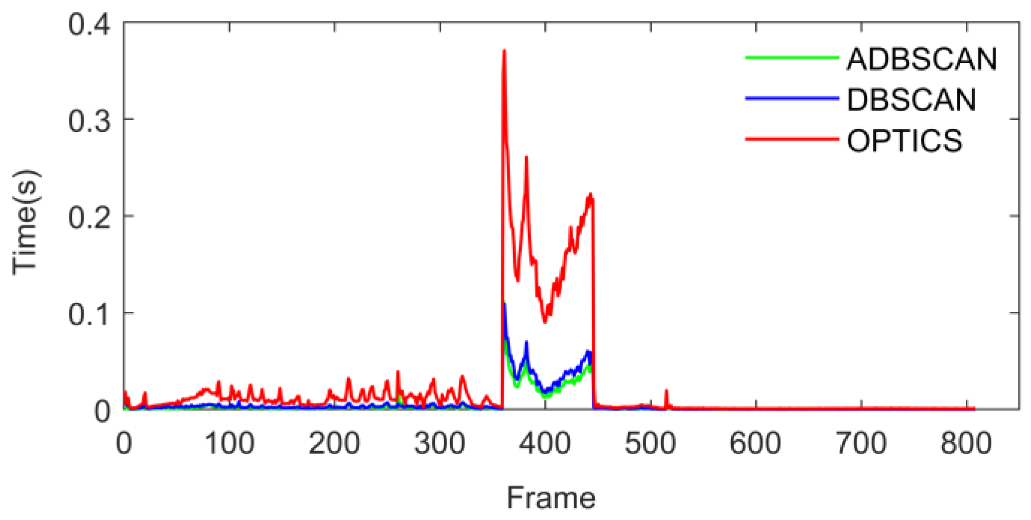
Figure 25 shows the time-consuming comparison of the three types of algorithms in each data set in the MATLAB environment. The ADBSCAN algorithm optimized by the KD-Tree algorithm takes less time, while the OPTICS algorithm takes more time in most cases. In the DBSCAN algorithm and ADBSCAN algorithm, the clustering quality of the ADBSCAN algorithm designed in this paper is better than the traditional DBSCAN algorithm, comparable to the OPTICS algorithm, but the time consumption is significantly lower than that of the OPTICS algorithm. Thus, the proposed ADBSCAN algorithm has achieved a certain balance in terms of accuracy and time consumption, it can be selected as needed in actual working conditions.
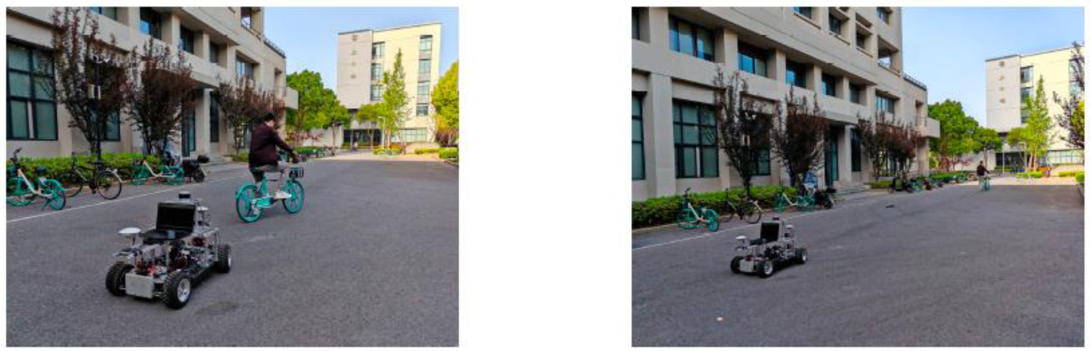
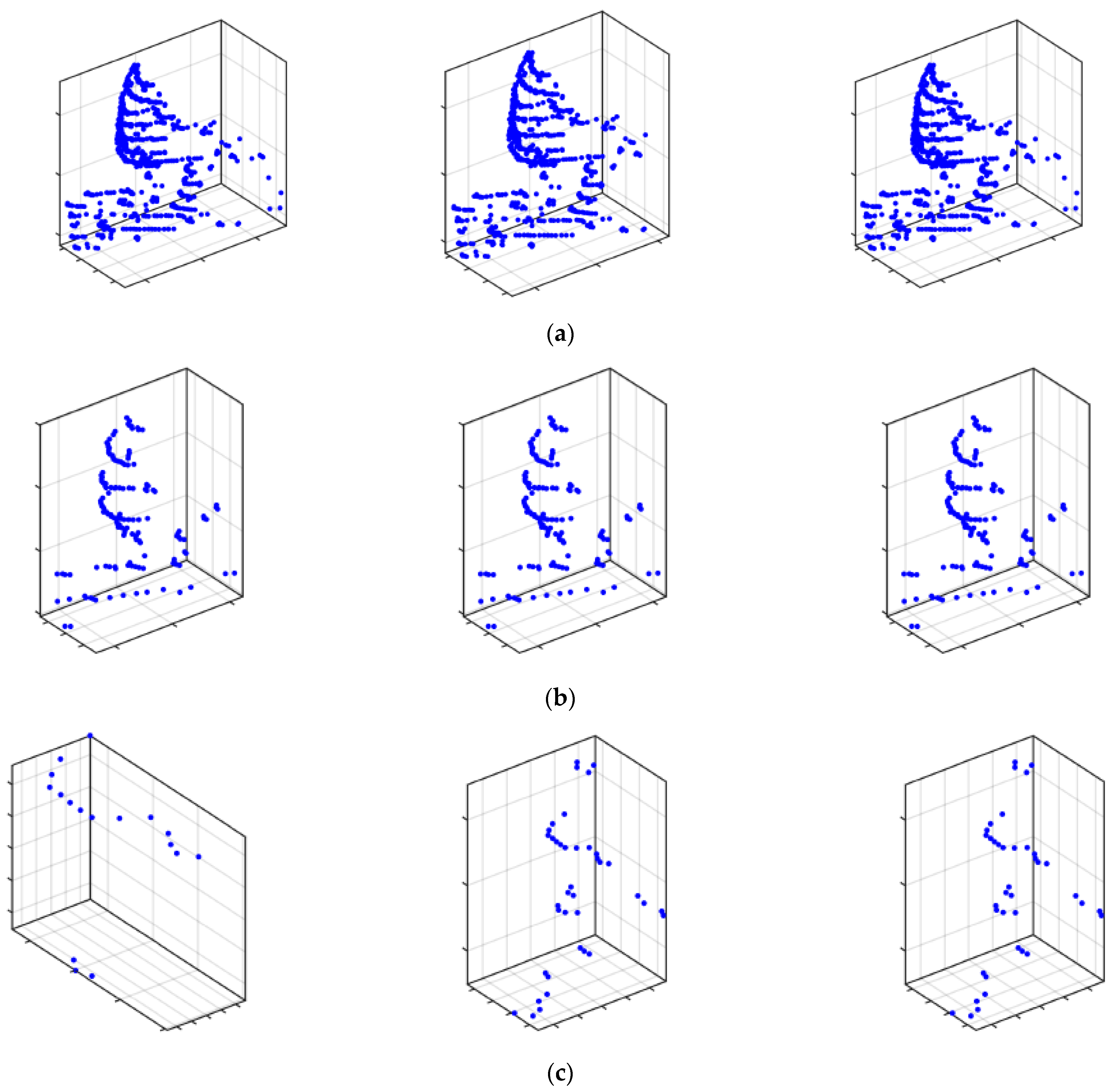
Quantitative experiments are carried out using the autonomous driving perception platform. As shown in Figure 26, the experimenters rode bicycles from near too far away until they exceeded the range of LiDAR clustering. Figure 27 shows the clustering effect of the algorithm at different distances. When the distance is 3 m, the clustering effect of the TDBSCAN algorithm and OPTICS algorithm is better than that of the ADBSCAN algorithm. When the distance reaches 6 m, the clustering effects of the three algorithms are all better. When the distance reaches 15 m, the TDBSCAN algorithm has lost the information in the height direction, but the ADBSCAN algorithm and the OPTICS algorithm still can guarantee normal clustering, which proves that the designed radius adaptive strategy is effective.
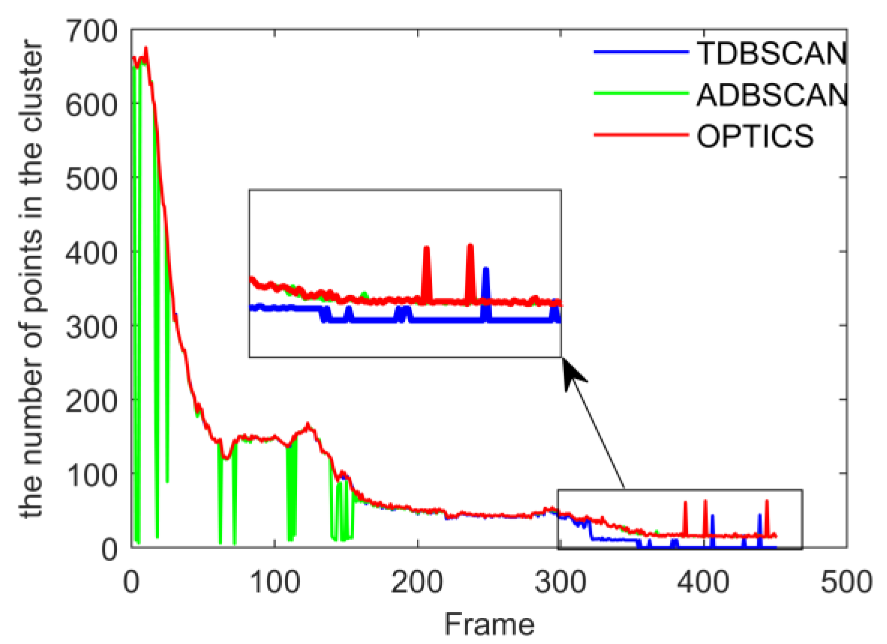
The comparison of the clustering quality of the three types of algorithms in 451 frames is shown in Figure 28. In the initial stage, the distance is relatively short, and the performance of the ADBSCAN algorithm proposed in this paper is poor and wrong clustering occurs. It is caused by setting the initial clustering radius to be small. The TDBSCAN algorithm and the OPTICS algorithm performed stably. After reaching 300 frames, the performance of the DBSCAN algorithm began to decline significantly, while the OPTICS algorithm and the ADBSCAN algorithm still maintained stable clustering.
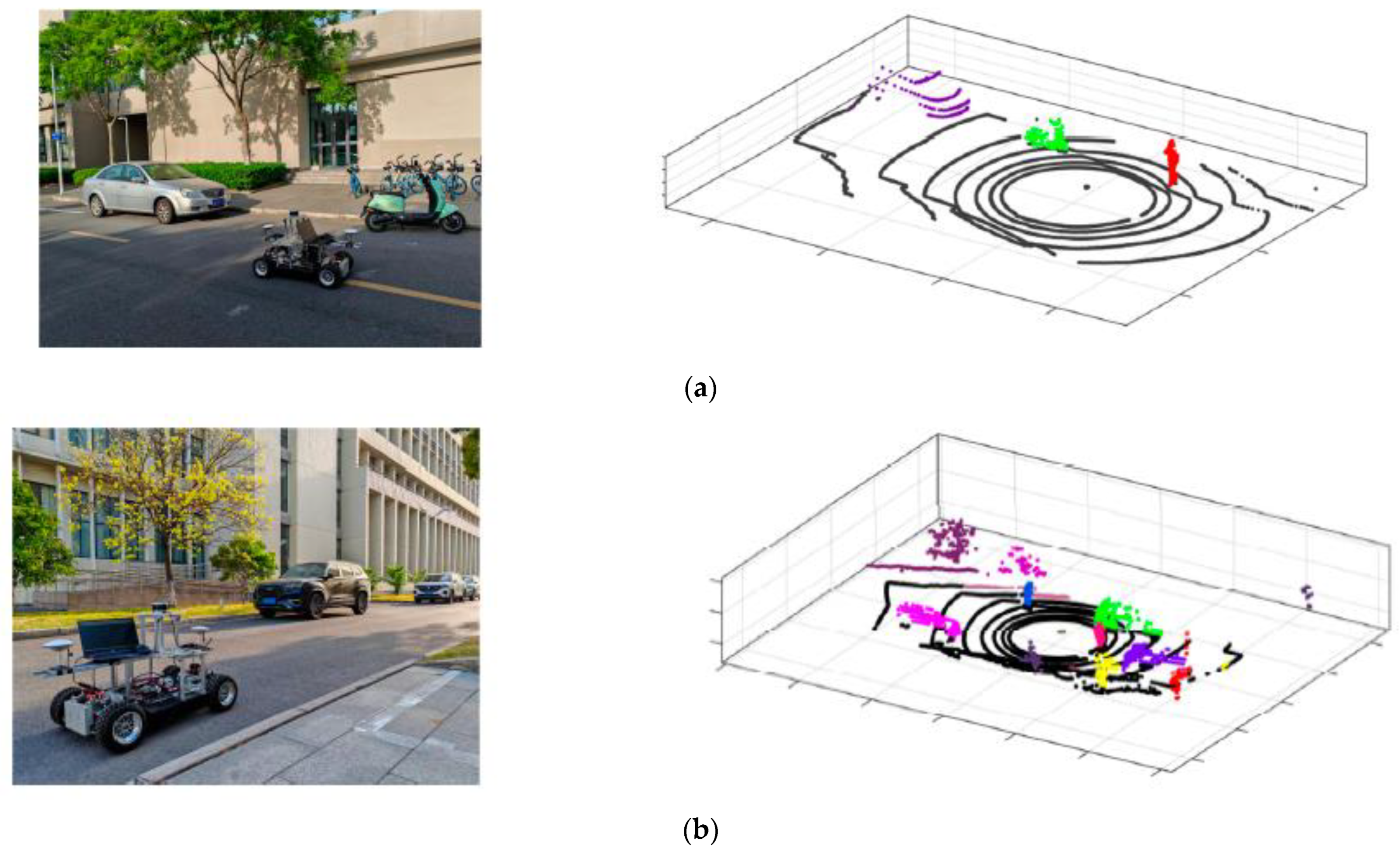
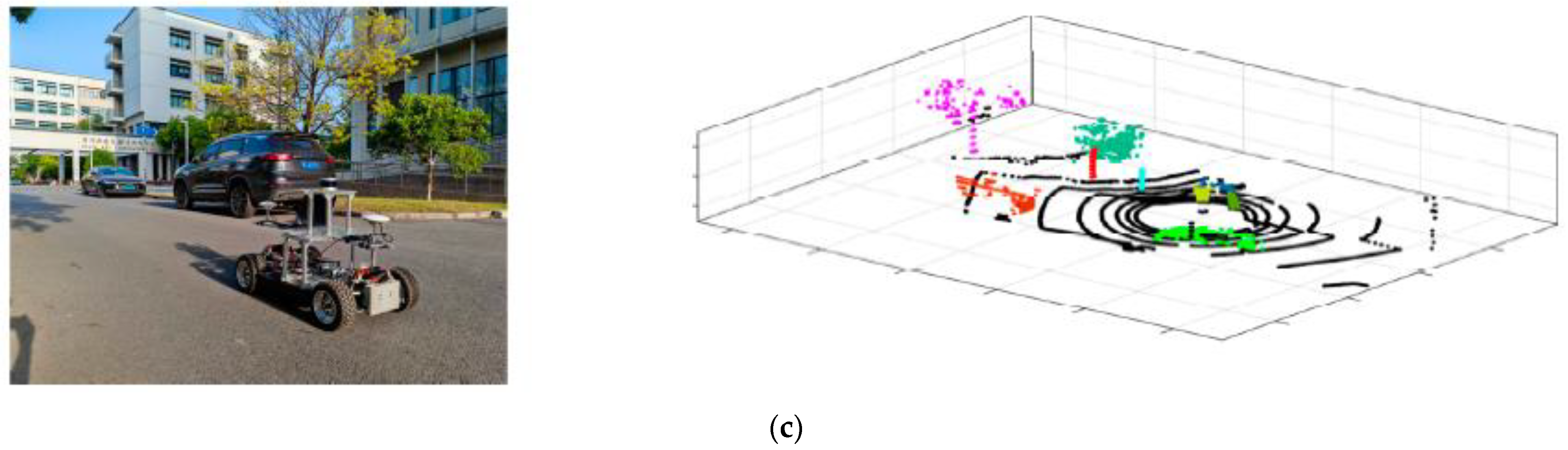
Figure 29 shows the clustering results of campus roads. Under different environments, the proposed ADBSCAN algorithm has a stable clustering effect.
4.2. Validation of Bounding Box Fitting Algorithm
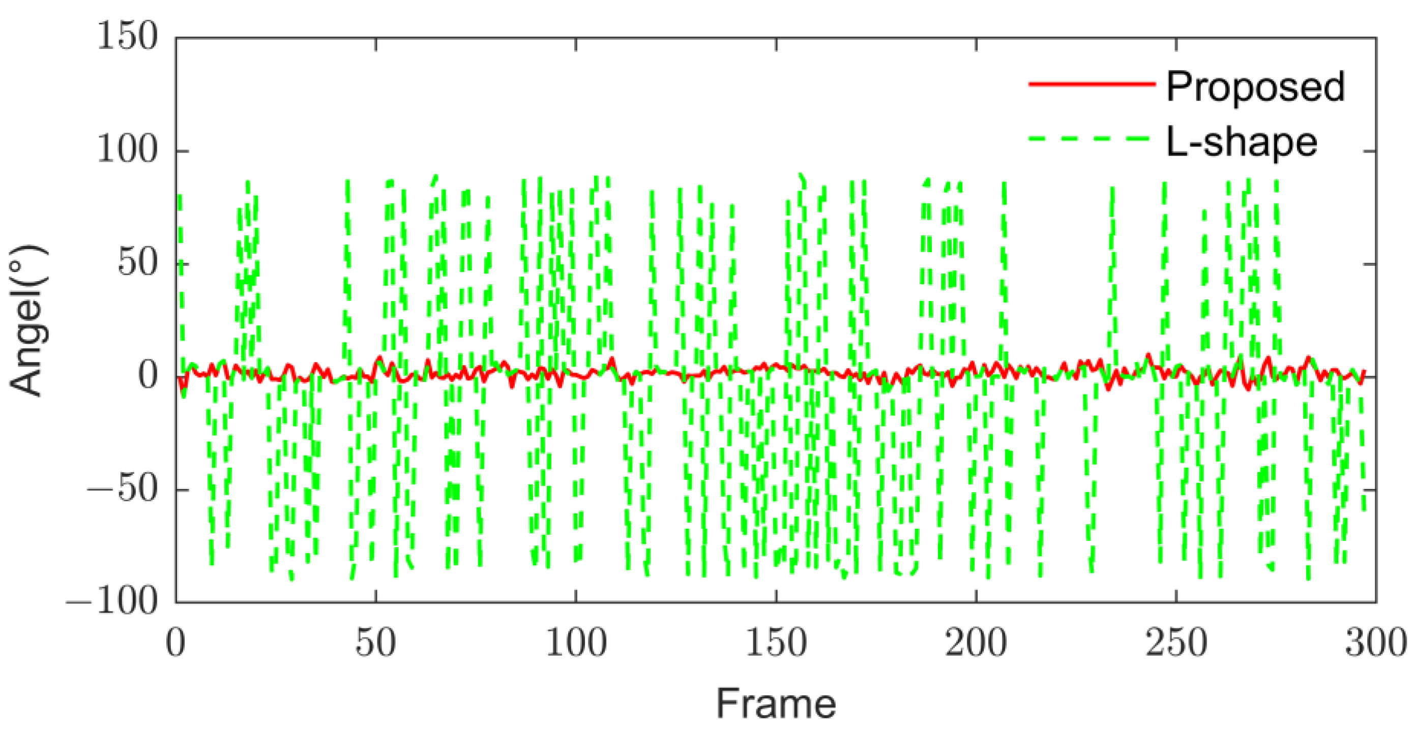
Since the algorithm verification platform has a poor detection effect on vehicles, only the KITTI dataset is used for verification. In data set 0056, the target is always in front of the smart car and basically keeps driving in a straight line. The comparison results of the direct estimation of the vehicle by the two algorithms are shown in Figure 30. The L-shape algorithm, which only considers the L-shaped contour points, shows a sharp fluctuation in the direction estimation, which is due to the misjudgment of the U shape as an L shape, resulting in a wrong direction judgment. In contrast, the orientation fit in the proposed algorithm has only small fluctuations caused by angle estimation errors. In 297 frames of point cloud data, the correct rate of shape judgment of the conventional algorithm is 35.2%, which is basically in a state of failure, while the correct rate of the proposed algorithm is 100%.
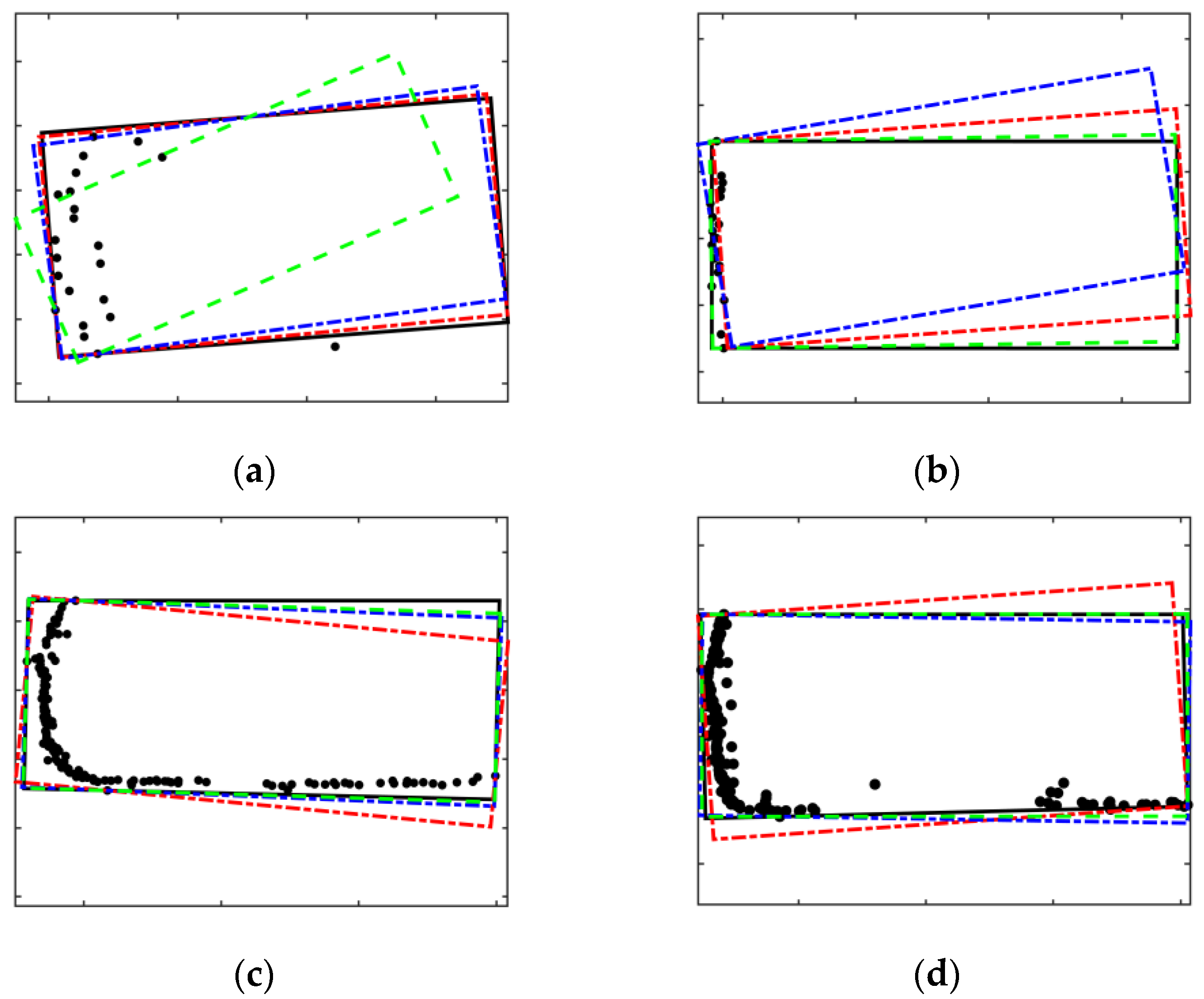
Next, the effectiveness of the RANSAC-PCA algorithm is further verified. The comparison algorithm is divided into three types, one is that all the fitting stages in the algorithm use the RANSAC algorithm, two is that all the fitting stages in the algorithm use the PCA algorithm and three is that all the fitting stages in the algorithm use the RANSAC algorithm twice. Figure 31 qualitatively shows the comparison of the fitting results of the four types of algorithms for different vehicle contour points. The black solid line in the figure represents the fitting result of the L-shaped algorithm using RANSCA-PCA straight line fitting, and the blue and red dotted lines represent the fitting results of the L-shape algorithm using one-time RANSAC and two-time RANSAC for straight-line fitting, respectively. The green dotted line represents the fitting result of the L-shape algorithm using PCA. It can be seen from Figure 31a that due to strong randomness, there are large deviations in the fitting results of the two separate RANSAC algorithms. After using the RANSAC algorithm twice for fitting, the results are significantly improved. In Figure 31b, the distribution of points is rather messy, and currently, the fitting using the PCA algorithm is basically in a state of failure. Figure 31c,d qualitatively shows the fitting results of the more standard L-shaped contour points, and all four types of algorithms can complete the bounding box fitting.
Table 4 shows the fitting results of the algorithm on four KITTI datasets. In each dataset, only one car is selected for statistical fitting, and the center point of the bounding box is calculated using the vehicle length and width data in the KITTI dataset as the ground truth. The accuracy of the proposed method is higher than that of the traditional L-shaped algorithm. Among them, the lateral error is small, mainly because the lateral direction of the target vehicle is easier to scan than the vertical direction; the estimation accuracy of the longitudinal length depends on the angle between the vehicle and the target vehicle, and the estimation is more difficult.
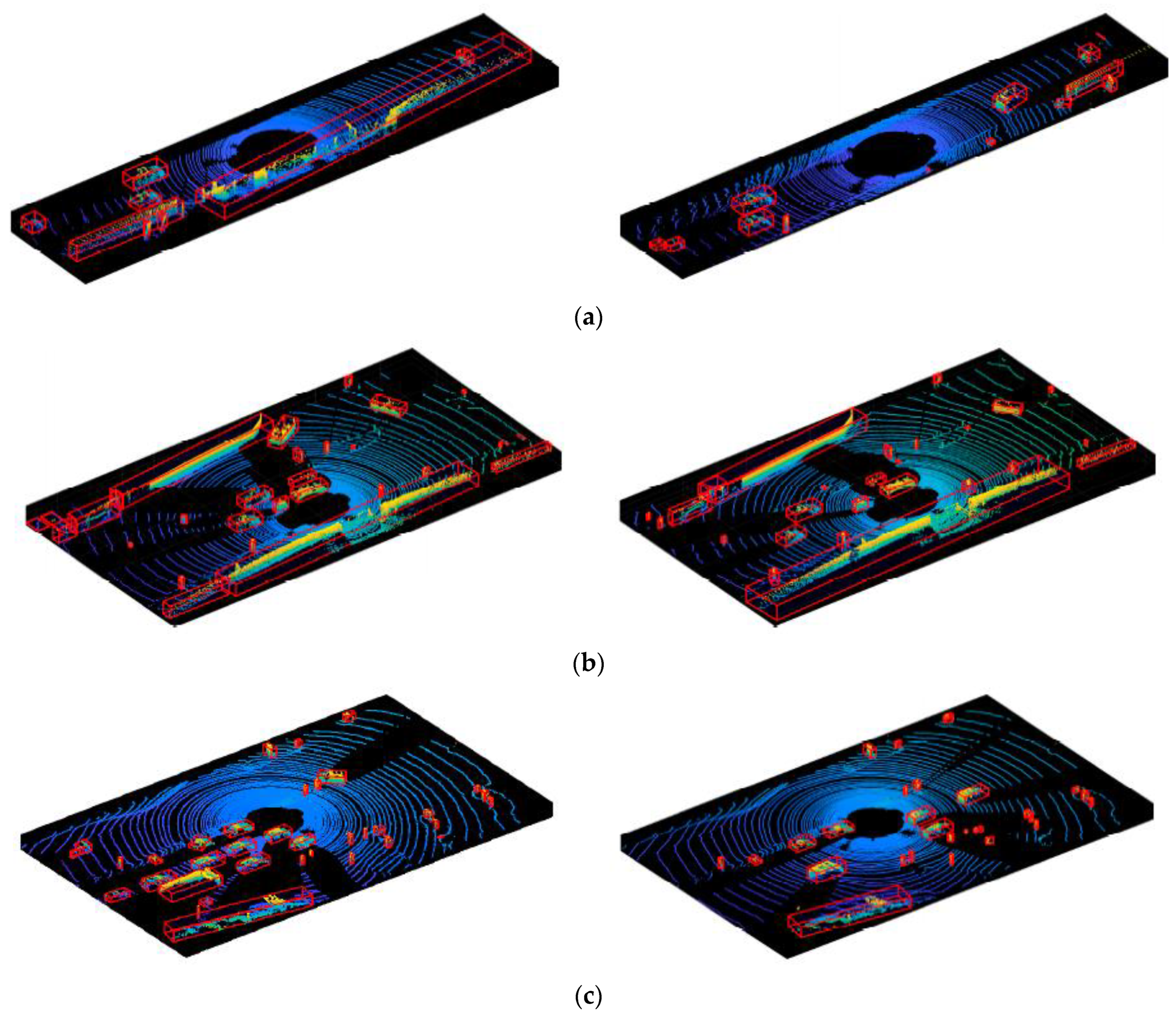
Figure 32 shows the results of clustering and bounding box fitting under different datasets.
4.3. Verification of Comprehensive Detection and Identification Results
After obtaining the preliminary screening results, it uses the trained PointNet point cloud classification network for vehicle recognition in this paper. The inputs are the cluster clusters that have not been screened by the bounding box and the high-confidence vehicle point cloud clusters that have been screened by the bounding box. The evaluation criteria are the precision rate P, the recall rate R and the F value, where the precision rate is defined as the proportion of positive predictions to all positive predictions:
The F and R is defined as
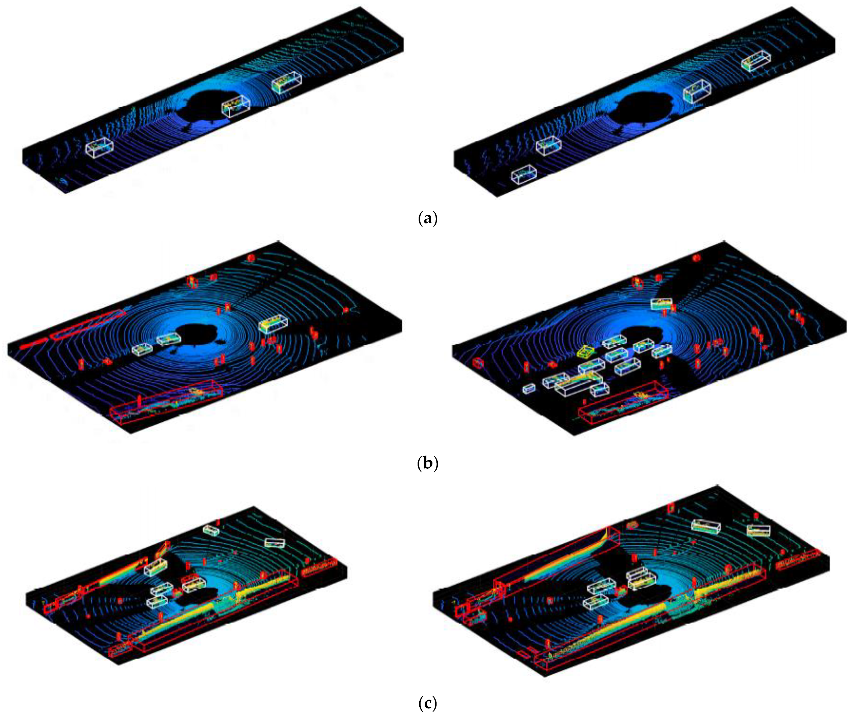
In the above formulas, TP means that the positive objects are predicted to be positive, FP means that the positive objects are predicted to be negative, TN means that the negative objects are predicted to be negative and FN means that the negative objects are predicted to be positive. Some detection results are shown in Figure 33.
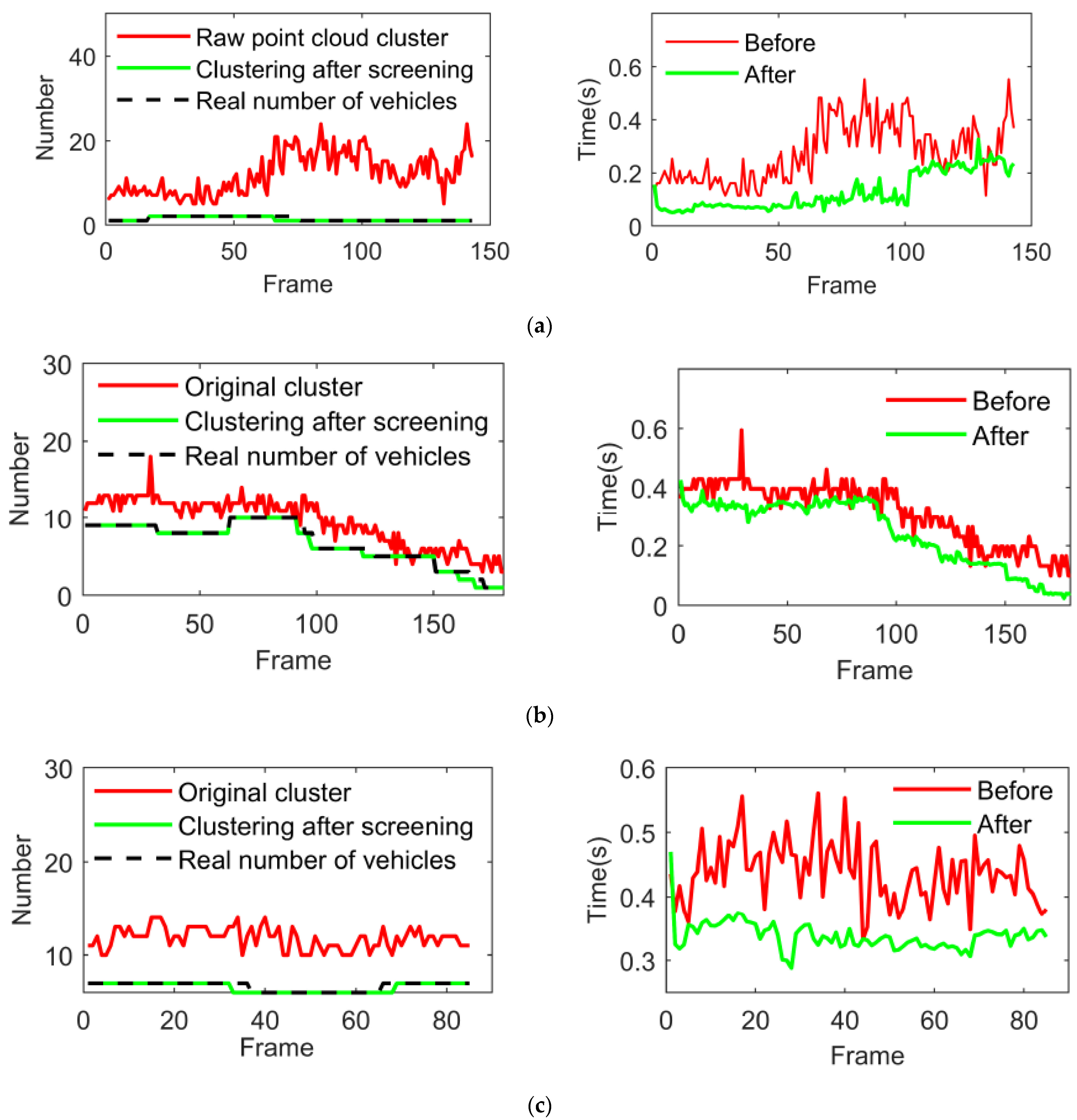
In Figure 33b, the bounding box fails and is marked yellow, but the PointNet algorithm still recognizes it as a vehicle at the end, indicating that the proposed algorithm framework has a certain fault tolerance rate. The front and rear algorithms can complement each other, and finally, vehicle object recognition is completed. The accuracy rate, recall rate and F value obtained by testing the three data sets are shown in Table 5. In the 0013 data set with a relatively simple scene, no matter whether the original cluster or the high-confidence vehicle cluster is input, the accuracy and the rates are higher, but it can be seen from Figure 33a that the proposed framework is less time-consuming. From the comparison of the recall rate R, the number of real vehicles is not significantly reduced after the initial screening of the bounding box. Therefore, the framework proposed in this paper is reliable and can stably identify vehicle targets.
The comparison of the number of point cloud clusters and the time-consuming comparison is shown in Figure 34. In the data set 0013, the bounding box can be selected as a candidate vehicle target most of the time, and the input after screening at frame 65 becomes 1, while the number of vehicles manually marked becomes 1 at frame 70. However, the vehicle point cloud is almost completely occluded between frame 65 and frame 70, and the vehicle cannot be recognized even if the original cluster is input. In terms of time consumption, when the number of clusters decreases significantly, the time consumption of the identification stage also decreases significantly, which proves that the use of bounding boxes to judge candidate vehicles in this paper can effectively reduce the time consumption of identification.
5. Conclusions and Future Work
A vehicle detection algorithm combining clustering results with deep learning is proposed to ensure robust vehicle point cloud detection in this paper. In the clustering part, the article proposes the ADBSCAN algorithm based on distance adaptive clustering radius to improve the problem of poor clustering effect under the condition of the distant sparse point cloud. In addition, the possibility of applying the OPTICS algorithm to vehicle point cloud clustering is also explored. After obtaining the clustering results, a vehicle bounding box fitting algorithm that can adapt to a variety of different vehicle profiles is presented, in which the principal component analysis algorithm is introduced into the line fitting process to ensure the robustness of the bounding box fitting. In the recognition part, a Point-Net point cloud classification network based on deep learning is constructed, and the obtained high-confidence vehicle bounding box is sent to PointNet for semantic recognition. Experiments based on the autonomous driving perception platform and the KITTI dataset prove that the detection framework can detect vehicle targets stably and has high robustness.
However, due to the limitations of experimental conditions, this paper only considers experimental validation for the robustness and reliability of the recognition framework, and the recognition accuracy of the entire framework can be probably further improved. The work will be carried out on the real vehicle in the future, and the real-time performance and accuracy of the framework will be optimized.
Author Contributions
Conceptualization, X.J., H.Y., X.H., G.L., Z.Y. and Q.W.; supervision, X.J. and X.H.; conception and design, X.J. and H.Y.; collection and assembly of data, X.J., H.Y. and Z.Y.; manuscript writing, X.J. and H.Y.; funding, X.J. and X.H. All authors have read and agreed to the published version of the manuscript.
Funding
National Key Research and Development Program of China under Grant 2022YFD2001405, National Modern Agricultural Industrial Technology System of China under Grant CARS-28-20, 2115 Talent Development Program of China Agricultural University and Foundation for State Key Laboratory of Automotive Simulation and Control under Grant 20181112.
Data Availability Statement
Not applicable.
Conflicts of Interest
The authors declare no conflict of interest.
References
- Wang, Z.; Zhan, J.; Duan, C.; Guan, X.; Lu, P.; Yang, K. A review of vehicle detection techniques for intelligent vehicles. IEEE Trans. Neural Netw. Learn. Syst. 2022, 1–21. [Google Scholar] [CrossRef] [PubMed]
- Jin, X.; Wang, J.; He, X.; Yan, Z.; Xu, L.; Wei, C.; Yin, G. Improving Vibration Performance of Electric Vehicles Based on In-Wheel Motor-Active Suspension System via Robust Finite Frequency Control. IEEE Trans. Intell. Transp. Syst. 2023, 24, 1631–1643. [Google Scholar] [CrossRef]
- Jin, X.; Wang, Q.; Yan, Z.; Yang, H. Nonlinear robust control of trajectory-following for autonomous ground electric vehicles with active front steering system. AIMS Math. 2023, 8, 11151–11179. [Google Scholar] [CrossRef]
- Jin, X.; Wang, J.; Yan, Z.; Xu, L.; Yin, G.; Chen, N. Robust vibration control for active suspension system of in-wheel-motor-driven electric vehicle via μ-synthesis methodology. ASME Trans. J. Dyn. Syst. Meas. Control. 2022, 144, 051007. [Google Scholar] [CrossRef]
- Xia, X.; Meng, Z.; Han, X.; Li, H.; Tsukiji, T.; Xu, R.; Zheng, Z.; Ma, J. An automated driving systems data acquisition and analytics platform. Transp. Res. Part C Emerg. Technol. 2023, 151, 104120. [Google Scholar] [CrossRef]
- Liu, W.; Quijano, K.; Crawford, M.M. YOLOv5-Tassel: Detecting tassels in RGB UAV imagery with improved YOLOv5 based on transfer learning. IEEE J. Sel. Top. Appl. Earth Obs. Remote Sens. 2022, 15, 8085–8094. [Google Scholar] [CrossRef]
- Monisha, A.A.; Reshmi, T.; Murugan, K. ERNSS-MCC: Efficient relay node selection scheme for mission critical communication using machine learning in VANET. Peer-to-Peer Netw. Appl. 2023, 1–24. [Google Scholar] [CrossRef]
- Kingston Roberts, M.; Thangavel, J. An improved optimal energy aware data availability approach for secure clustering and routing in wireless sensor networks. Trans. Emerg. Telecommun. Technol. 2023, 34, e4711. [Google Scholar] [CrossRef]
- So, J.; Hwangbo, J.; Kim, S.H.; Yun, I. Analysis on autonomous vehicle detection performance according to various road geometry settings. J. Intell. Transp. Syst. 2022, 27, 384–395. [Google Scholar] [CrossRef]
- Ali, W.; Abdelkarim, S.; Zidan, M.; Zahran, M.; El Sallab, A. Yolo3d: End-to-end real-time 3d oriented object bounding box detection from lidar point cloud. In Proceedings of the European Conference on Computer Vision (ECCV) Workshops, Munich, Germany, 8–14 September 2018; pp. 716–728. [Google Scholar]
- Yang, B.; Luo, W.; Urtasun, R. Pixor: Real-time 3d object detection from point clouds. In Proceedings of the IEEE Conference on Computer Vision and Pattern Recognition(CVPR), Salt Lake, UT, USA, 18–22 June 2018; pp. 7652–7660. [Google Scholar]
- Qi, C.R.; Su, H.; Mo, K.; Guibas, L.J. Pointnet: Deep learning on point sets for 3d classification and segmentation. In Proceedings of the IEEE Conference on Computer Vision and Pattern Recognition(CVPR), Honolulu, HS, USA, 21–26 July 2017; pp. 652–660. [Google Scholar]
- Shi, S.; Guo, C.; Jiang, L.; Wang, Z.; Shi, J.; Wang, X.; Li, H. Pv-rcnn: Point-voxel feature set abstraction for 3d object detection. In Proceedings of the IEEE/CVF Conference on Computer Vision and Pattern Recognition(CVPR), Seattle, WA, USA, 14–19 June 2020; pp. 10529–10538. [Google Scholar]
- Li, Z.; Wang, F.; Wang, N. Lidar r-cnn: An efficient and universal 3d object detector. In Proceedings of the IEEE/CVF Conference on Computer Vision and Pattern Recognition(CVPR), Nashville, TN, USA, 19–25 June 2021; pp. 7546–7555. [Google Scholar]
- Zhou, Y.; Tuzel, O. Voxelnet: End-to-end learning for point cloud based 3d object detection. In Proceedings of the IEEE Conference on Computer Vision and Pattern Recognition(CVPR), Salt Lake, UT, USA, 18–22 June 2018; pp. 4490–4499. [Google Scholar]
- Yan, Y.; Mao, Y.; Li, B. Second: Sparsely embedded convolutional detection. Sensors 2018, 18, 3337. [Google Scholar] [CrossRef] [Green Version]
- Deng, J.; Shi, S.; Li, P.; Zhou, W.; Zhang, Y.; Li, H. Voxel r-cnn: Towards high performance voxel-based 3d object detection. In Proceedings of the AAAI Conference on Artificial Intelligence(AAAI), Vancouver, BC, Canada, 2–9 February 2021; pp. 1201–1209. [Google Scholar]
- Chen, H.; Liang, M.; Liu, W.; Wang, W.; Liu, P.X. An approach to boundary detection for 3D point clouds based on DBSCAN clustering. Pattern Recognit. 2022, 124, 108431. [Google Scholar] [CrossRef]
- Wang, C.; Ji, M.; Wang, J.; Wen, W.; Li, T.; Sun, Y. An improved DBSCAN method for LiDAR data segmentation with automatic Eps estimation. Sensors 2019, 19, 172. [Google Scholar] [CrossRef] [PubMed] [Green Version]
- Gao, J.; Chen, Y.; Junior, J.M.; Wang, C.; Li, J. Rapid extraction of urban road guardrails from mobile LiDAR point clouds. IEEE Trans. Intell. Transp. Syst. 2020, 23, 1572–1577. [Google Scholar] [CrossRef]
- Miao, Y.; Tang, Y.; Alzahrani, B.A.; Barnawi, A.; Alafif, T.; Hu, L. Airborne LiDAR assisted obstacle recognition and intrusion detection towards unmanned aerial vehicle: Architecture, modeling and evaluation. IEEE Trans. Intell. Transp. Syst. 2020, 22, 4531–4540. [Google Scholar] [CrossRef]
- El Yabroudi, M.; Awedat, K.; Chabaan, R.C.; Abudayyeh, O.; Abdel-Qader, I. Adaptive DBSCAN LiDAR Point Cloud Clustering For Autonomous Driving Applications. In Proceedings of the 2022 IEEE International Conference on Electro Information Technology (eIT), Mankato, MN, USA, 19–21 May 2022; pp. 221–224. [Google Scholar]
- Wen, L.; He, L.; Gao, Z. Research on 3D Point Cloud De-Distortion Algorithm and Its Application on Euclidean Clustering. IEEE Access 2019, 7, 86041–86053. [Google Scholar] [CrossRef]
- Zhang, X.; Xu, W.; Dong, C.; Dolan, J.M. Efficient L-shape fitting for vehicle detection using laser scanners. In Proceedings of the 2017 IEEE Intelligent Vehicles Symposium (IV), Redondo Beach, CA, USA, 11–14 June 2017; pp. 54–59. [Google Scholar]
- Zhao, C.; Fu, C.; Dolan, J.M.; Wang, J. L-shape fitting-based vehicle pose estimation and tracking using 3D-LiDAR. IEEE Trans. Intell. Veh. 2021, 6, 787–798. [Google Scholar] [CrossRef]
- Kim, D.; Jo, K.; Lee, M.; Sunwoo, M. L-shape model switching-based precise motion tracking of moving vehicles using laser scanners. IEEE Trans. Intell. Transp. Syst. 2017, 19, 598–612. [Google Scholar] [CrossRef]
- Sun, P.; Zhao, X.; Xu, Z.; Wang, R.; Min, H. A 3D LiDAR data-based dedicated road boundary detection algorithm for autonomous vehicles. IEEE Access 2019, 7, 29623–29638. [Google Scholar] [CrossRef]
- Guo, G.; Zhao, S. 3D multi-object tracking with adaptive cubature Kalman filter for autonomous driving. IEEE Trans. Intell. Veh. 2022, 8, 512–519. [Google Scholar] [CrossRef]
- Liu, K.; Wang, W.; Tharmarasa, R.; Wang, J. Dynamic vehicle detection with sparse point clouds based on PE-CPD. IEEE Trans. Intell. Transp. Syst. 2018, 20, 1964–1977. [Google Scholar] [CrossRef]
- Kim, T.; Park, T.-H. Extended Kalman filter (EKF) design for vehicle position tracking using reliability function of radar and lidar. Sensors 2020, 20, 4126. [Google Scholar] [CrossRef]
- Golovinskiy, A.; Kim, V.G.; Funkhouser, T. Shape-based recognition of 3D point clouds in urban environments. In Proceedings of the 2009 IEEE 12th International Conference on Computer Vision(ICCV), Kyoto, Japan, 1–2 October 2009; pp. 2154–2161. [Google Scholar]
- Chen, T.; Dai, B.; Wang, R.; Liu, D. Gaussian-process-based real-time ground segmentation for autonomous land vehicles. J. Intell. Robot. Syst. 2014, 76, 563–582. [Google Scholar] [CrossRef]
- Eum, J.; Bae, M.; Jeon, J.; Lee, H.; Oh, S.; Lee, M. Vehicle detection from airborne LiDAR point clouds based on a decision tree algorithm with horizontal and vertical features. Remote Sens. 2017, 8, 409–418. [Google Scholar] [CrossRef]
- Jin, X.; Yang, H.; Liao, X.; Yan, Z.; Wang, Q.; Li, Z.; Wang, Z. A Robust Gaussian Process-Based LiDAR Ground Segmentation Algorithm for Autonomous Driving. Machines 2022, 10, 507. [Google Scholar] [CrossRef]
Figure 1.
Technical framework of proposed vehicle detection.

Figure 2.
Schematic of DBSCAN algorithm.

Figure 3.
LiDAR planar scan model.

Figure 4.
KD-Tree construction process.

Figure 5.
The flow of proposed DBSCAN algorithm.

Figure 6.
The relationship between the parameters.

Figure 7.
L-shape bounding box fitting algorithm.

Figure 8.
Common angle judgment fails. (a) Long and short side fitting failure (b) Short side fitting failure (c) Angle too small (d) Long and short side fitting failure.
Figure 8.
Common angle judgment fails. (a) Long and short side fitting failure (b) Short side fitting failure (c) Angle too small (d) Long and short side fitting failure.

Figure 9.
Common three types of vehicles point cloud contours.

Figure 10.
Schematic of judging U-shaped and L-shaped contours.

Figure 11.
Comparison of fitting results between PCA algorithm and RANSAC algorithm. (a) There are outliers but the data distribution is linear. (b) There are no outliers but the data distribution is nonlinear.
Figure 11.
Comparison of fitting results between PCA algorithm and RANSAC algorithm. (a) There are outliers but the data distribution is linear. (b) There are no outliers but the data distribution is nonlinear.

Figure 12.
The process of the bounding box fitting algorithm.

Figure 13.
Bounding box before and after filtering.

Figure 14.
3D convolution process.

Figure 15.
Pooling in two different ways.

Figure 16.
PointNet classification network structure.

Figure 17.
T-Net alignment network.

Figure 18.
Multilayer perceptron.

Figure 19.
Different types of targets. (a) Car, (b) Cyclist, (c) Another car, (d) Pedestrian, (e) Truck and (f) Van.
Figure 19.
Different types of targets. (a) Car, (b) Cyclist, (c) Another car, (d) Pedestrian, (e) Truck and (f) Van.

Figure 20.
Sample after data processing. (a) Raw data, (b) Zero padding, (c) Data normalization.

Figure 21.
Autonomous Driving Perception Platform.

Figure 22.
KITTI dataset 2011_09_26_0013 point cloud clustering effect.

Figure 23.
Comparison of clustering results for each obstacle.

Figure 24.
Comparison of clustering results of three types of algorithms.

Figure 25.
Time-consuming comparison of different clustering algorithms.

Figure 26.
Test site and scene.

Figure 27.
Schemes follow the same formatting. (a) Clustering effect at 3 m (the number of cluster points is 660, 649 and 660). (b) Clustering effect at 6 m (the number of cluster points is 148, 148 and 148). (c) Clustering effect at 15 m (number of cluster points 17, 39 and 39).
Figure 27.
Schemes follow the same formatting. (a) Clustering effect at 3 m (the number of cluster points is 660, 649 and 660). (b) Clustering effect at 6 m (the number of cluster points is 148, 148 and 148). (c) Clustering effect at 15 m (number of cluster points 17, 39 and 39).

Figure 28.
Clustering quality comparison.

Figure 29.
Clustering results in different campus scenarios. (a) Campus scene 1. (b) Campus scene 2. (c) Campus scene 3.
Figure 29.
Clustering results in different campus scenarios. (a) Campus scene 1. (b) Campus scene 2. (c) Campus scene 3.


Figure 30.
Angle Estimation Comparison.

Figure 31.
Robustness comparison of the algorithm under different types of vehicle contours. (a) Comparison of U-shaped profile fitting results 1. (b) Comparison of U-shaped profile fitting results 2. (c) Comparison of L-shaped profile fitting results 1. (d) Comparison of L-shaped profile fitting results 2.

Figure 32.
Clustering and fitting results in different dataset. (a) dataset 0013, (b) dataset 0020, (c) dataset 0018.
Figure 32.
Clustering and fitting results in different dataset. (a) dataset 0013, (b) dataset 0020, (c) dataset 0018.

Figure 33.
Bounding box fitting and recognition results in different datasets. (a) dataset 0013, (b) dataset 0018 and (c) dataset 0020.
Figure 33.
Bounding box fitting and recognition results in different datasets. (a) dataset 0013, (b) dataset 0018 and (c) dataset 0020.

Figure 34.
Robustness comparison of the algorithm under different types of vehicle contours. (a) Comparison of the number of candidates point cloud clusters and time-consuming in dataset 0013. (b) Comparison of the number of candidates point cloud clusters and time-consuming in dataset 0018. (c) Comparison of the number of candidates point cloud clusters and time-consuming in dataset 0020.


Table 1.
Bounding box initial screening index.
| Number | Threshold | Definition |
|---|---|---|
| 1 | Maximum and minimum height of obstacles | |
| 2 | Maximum and minimum width of obstacles | |
| 3 | Maximum and minimum length of obstacles | |
| 4 | Top View Area of Obstacles | |
| 5 | The aspect ratio of the obstacle | |
| 6 | Aspect ratio threshold for obstacles | |
| 7 | The number of points contained within the obstacle |
Table 2.
Comparison of the number and proportion of samples of each category before and after data enhancement.
Table 2.
Comparison of the number and proportion of samples of each category before and after data enhancement.
| Class | Index | Car | Cyclist | Pedestrian | Other |
|---|---|---|---|---|---|
| Before | Number | 10,341 | 1595 | 4767 | 1863 |
| Ratio | 55.69% | 8.59% | 25.67% | 10.03% | |
| After | Number | 8632 | 5403 | 6093 | 5023 |
| Ratio | 34.3% | 21.48% | 24.23% | 19.97% |
Table 3.
Comparison of clustering quality of each clustering algorithm.
| Serial Number | Algorithm | Correct Frame | Wrong Frame | Right Ratio |
|---|---|---|---|---|
| 0004 | DBSCAN | 173 | 86 | 66.8% |
| ADBSCAN | 248 | 11 | 96.50% | |
| OPTICS | 257 | 2 | 99.22% | |
| 0018 | DBSCAN | 66 | 34 | 66% |
| ADBSCAN | 89 | 11 | 89% | |
| OPTICS | 82 | 18 | 82% | |
| 0020 | DBSCAN | 55 | 31 | 63.95% |
| ADBSCAN | 61 | 25 | 70.93% | |
| OPTICS | 80 | 6 | 93.02% | |
| 0026 | DBSCAN | 50 | 17 | 74.63% |
| ADBSCAN | 62 | 5 | 92.54% | |
| OPTICS | 67 | 2 | 97.1% | |
| 0056 | DBSCAN | 258 | 36 | 87.76% |
| ADBSCAN | 284 | 10 | 96.6% | |
| OPTICS | 294 | 0 | 100% |
Table 4.
Algorithm comparison results on the KITTI dataset (meters).
| Serial Number | Algorithm | Horizontal | Vertical | ||
|---|---|---|---|---|---|
| Mean | Variance | Mean | Variance | ||
| 0001 | Regular | 0.0986 | 0.056 | 0.1435 | 0.1368 |
| Proposed | 0.0688 | 0.0458 | 0.1143 | 0.1415 | |
| 0015 | Regular | 0.1191 | 0.0935 | 0.515 | 0.135 |
| Proposed | 0.0912 | 0.0721 | 0.265 | 0.126 | |
| 0020 | Regular | 0.0742 | 0.0749 | 0.3979 | 0.1288 |
| Proposed | 0.0652 | 0.0689 | 0.2950 | 0.132 | |
| 0032 | Regular | 0.1065 | 0.0912 | 0.3998 | 0.251 |
| Proposed | 0.0842 | 0.0688 | 0.2829 | 0.299 | |
Table 5.
Recognition Algorithm Performance Comparison.
| Algorithm | Dataset | Precision P | Recall R | F |
|---|---|---|---|---|
| Regular | 0013 | 0.926 | 0.846 | 0.884 |
| 0018 | 0.903 | 0.861 | 0.882 | |
| 0026 | 0.891 | 0.847 | 0.868 | |
| Proposed | 0013 | 0.982 | 0.864 | 0.919 |
| 0018 | 0.965 | 0.904 | 0.934 | |
| 0026 | 0.943 | 0.901 | 0.922 |
Disclaimer/Publisher’s Note: The statements, opinions and data contained in all publications are solely those of the individual author(s) and contributor(s) and not of MDPI and/or the editor(s). MDPI and/or the editor(s) disclaim responsibility for any injury to people or property resulting from any ideas, methods, instructions or products referred to in the content. |
© 2023 by the authors. Licensee MDPI, Basel, Switzerland. This article is an open access article distributed under the terms and conditions of the Creative Commons Attribution (CC BY) license (https://creativecommons.org/licenses/by/4.0/).
Share and Cite
MDPI and ACS Style
Jin, X.; Yang, H.; He, X.; Liu, G.; Yan, Z.; Wang, Q. Robust LiDAR-Based Vehicle Detection for On-Road Autonomous Driving. Remote Sens. 2023, 15, 3160. https://doi.org/10.3390/rs15123160
AMA Style
Jin X, Yang H, He X, Liu G, Yan Z, Wang Q. Robust LiDAR-Based Vehicle Detection for On-Road Autonomous Driving. Remote Sensing. 2023; 15(12):3160. https://doi.org/10.3390/rs15123160
Chicago/Turabian StyleJin, Xianjian, Hang Yang, Xiongkui He, Guohua Liu, Zeyuan Yan, and Qikang Wang. 2023. "Robust LiDAR-Based Vehicle Detection for On-Road Autonomous Driving" Remote Sensing 15, no. 12: 3160. https://doi.org/10.3390/rs15123160
Note that from the first issue of 2016, this journal uses article numbers instead of page numbers. See further details here.