Article

Elimination of Thermal Effects from Limited Structural Displacements Based on Remote Sensing by Machine Learning Techniques

1
Department of Civil and Environmental Engineering, Politecnico di Milano, Piazza L. da Vinci 32, 20133 Milano, Italy
2
Finnish Meteorological Institute (FMI), Erik Palménin Aukio 1, FI-00560 Helsinki, Finland
*
Author to whom correspondence should be addressed.
Remote Sens. 2023, 15(12), 3095; https://doi.org/10.3390/rs15123095
Submission received: 26 April 2023 / Revised: 27 May 2023 / Accepted: 7 June 2023 / Published: 13 June 2023
(This article belongs to the Special Issue Remote Sensing in Safety and Disaster Prevention Engineering)

Abstract

:
Confounding variability caused by environmental and/or operational conditions is a big challenge in the structural health monitoring (SHM) of large-scale civil structures. The elimination of such variability is of paramount importance in avoiding economic and human losses. Machine learning-aided data normalization provides a good solution to this challenge. Despite proper studies on data normalization using structural responses/features acquired from contact-based sensors, this issue has not been explored properly via new features, such as displacement responses from remote sensing products, including synthetic aperture radar (SAR) images. Hence, the main aim of this work was to eliminate environmental variability, particularly thermal effects, from different and limited structural displacements retrieved from a few SAR images related to long-term health monitoring programs of long-span bridges. For this purpose, we conducted a comprehensive comparative study to investigate two supervised and two unsupervised data normalization algorithms. The supervised algorithms were based on Gaussian process regression (GPR) and support vector regression (SVR), for which temperature records acquired from contact temperature sensors and structural displacements retrieved from spaceborne remote sensors produce univariate predictor (input) and response (output) data for the regression problem. For the unsupervised algorithms, this paper employed principal component analysis (PCA) and proposed a deep autoencoder (DAE), both of which conform with unsupervised reconstruction-based data normalization. In contrast to the GPR- and SVR-based data normalization algorithms, both the PCA and DAE methods only consider the SAR-based displacement (output) data without any requirement of the environmental and/or operational (input) data. Limited displacement sets of long-span bridges from a few SAR images of Sentinel-1A, related to long-term SHM programs, were considered to assess the aforementioned techniques. Results demonstrate that the proposed DAE-aided data normalization is the best approach to remove thermal effects and other unmeasured environmental and/or operational variability.

1. Introduction

The health monitoring of bridge structures is of utmost importance in every society due to their impacts on social life, transportation networks, commerce, etc. The occurrence of damage, failure, and even collapse may induce irreparable human deaths and extreme economical losses. To avoid any catastrophic event, structural health monitoring (SHM) has brought a great opportunity to preserve vital civil structures [1,2], particularly bridges [3,4,5]. Generally, an SHM program consists of some fundamental steps of sensing, feature extraction, and decision-making. Sensing is an important step of any SHM strategy by deploying the structure with different contact and non-contact sensors and data acquisition and transmission systems for measuring useful data [6]. In the context of vibration-based SHM, feature extraction utilizes the measured data in order to discover meaningful information (structural feature) relevant to damage. Eventually, decision-making applies the extracted information from the measured data to perform SHM tasks in terms of early damage detection, damage localization, and damage quantification.
Recently, the technology of remote sensing has highly assisted civil engineers and researchers in taking advantage of the capacity of synthetic aperture radar (SAR) images acquired from satellites for extracting displacements as the main structural features obtained using various interferometric techniques [7] and evaluating the health and integrity of civil structures [8]. One of the great advantages of remote sensing is the lack of installed contact sensors, in-site experiments/measurements, and climatic conditions, which makes it a cost-effective sensing technique for SHM. The other important merit of this technique is the possibility of obtaining prior information (archived images) of civil structures regarding their initial or undamaged states, while this characteristic is not simply possible in SHM applications. The last merit of the SAR-aided SHM is to cover large areas on the earth that allows civil engineers to capture useful information (e.g., structural responses in terms of vertical and horizontal displacements) on large-scale civil structures, such as long-span bridges.
Once the structural features have been obtained, decision-making can be implemented by different machine learning algorithms. In this regard, one can exploit the main learning algorithms, in terms of supervised learning and unsupervised learning [9], and leverage some advanced algorithms, which include but are not limited to deep learning [10], transfer learning [11], kernel learning [12], ensemble learning [13], empirical learning [14], meta-learning [15], multi-task learning [16], etc. Totally, these learning algorithms intend to develop computational models by using training data and then use the trained models for some tasks, such as classification, prediction, regression, clustering, and anomaly detection via test data.
Despite valuable research studies and practical projects on the SHM of various civil structures, some serious challenges are still problematic and some of them have not been studied comprehensively. Although the main objective of SHM is to diagnose structural damage in terms of early damage detection, damage localization, and damage quantification, variability in measured data or structural features may lead to critical decision-making errors, that is, false positives and false negatives. The first error means that the civil structure operates normally but the method incorrectly warns of the occurrence of damage leading to economic losses. The second error means that the structure suffered from damage but the variability in conditions masks adverse changes caused by damage leading to human losses. The significant variability in conditions in SHM are mainly caused by environmental and operational changes. In most cases, variations in temperature, humidity, wind characteristics, and live loads (e.g., traffic) are the major reasons for changes in the measured data or features extracted from such data (e.g., modal parameters [17], displacements extracted from SAR images [18,19]).
Among all environmental variability conditions, thermal effects caused by air temperature fluctuations and solar radiation are critical for long-term SHM projects. This is because such effects may induce excessive (thermal) loads, in addition to dead and live loads. In this case, large displacements and undesirable internal stresses are prevalent consequences. Such loads can also lead to cracks in structural elements and connections when those are restrained by fixed boundary conditions. In worse conditions, large deviations in a structure caused by damage may mistakenly be interpreted as a thermal response leading to collapse due to a false negative error [20,21]. On the other hand, temperature fluctuations in freezing conditions can temporarily increase the stiffness of civil structures [22], in which case, sharp increases in some structural features (i.e., modal frequencies) are highly confounding.
To alleviate the negative impacts of temperature variability and thermal loads, it is essential to remove their influences and provide normalized structural features. One of the significant characteristics of such features is that those are only relevant to structural changes and damage. In this case, any change in such features is indicative of an abnormal condition, such as damage. In the context of SHM, the removal of environmental and/or operational variability is often conducted using different machine learning-aided data normalization methods [23]. Depending upon the feasibility of measuring the environmental and operational conditions, data normalization approaches are divided into input–output and output-only categories. The first category requires the environmental and/or operational data (e.g., temperature records), which serve as the input, and the structural feature (e.g., modal frequencies or displacements), which is treated as the output. Based on the main concept of machine learning, the input–output data normalization techniques are developed from supervised regression models. By contrast, the second category is only dependent on the structural responses or features without any measuring of the environmental and operational data. From the machine learning viewpoint, the output-only data normalization techniques are based on unsupervised learning algorithms.
Despite valuable studies regarding data normalization for SHM applications, of which most have focused on dynamic features, such as modal frequencies extracted from structural responses (e.g., accelerations) and contact-based sensors, this issue has not been investigated properly via new structural responses/features and machine learning algorithms. Hence, this paper concentrates on structural displacements retrieved from spaceborne remote sensing and its products, i.e., SAR images, for eliminating thermal effects and other unmeasured environmental and/or operational conditions in long-term monitoring programs. One of the important challenges in applying SAR-based displacement responses compared to other structural responses/features (e.g., modal properties) is concerned with the dimension of features. In most cases, a long-monitoring scheme based on spaceborne remote sensing includes a few SAR images, in which case limited displacements are only available for data normalization. Thus, the performance of some state-of-the-art data normalization techniques with small data and new structural features (i.e., the displacements retrieved from remote sensing) needs further investigations.

1.1. Related Works

Because of the importance of data normalization in SHM, this section overviews some literature on this problem. In relation to the input–output (supervised) data normalization, regression models are the commonly-used techniques [24,25]. Laory et al. [26] applied artificial neural networks (ANNs), support vector regression (SVR), regression tree, and random forest to represent the relationship between temperature and modal frequencies (structural responses) of a long-span bridge. Jang and Smyth [27] used random forests, ANNs, and SVR to numerically study the effects of temperature on the modal frequencies of a cable-stayed bridge. Ma et al. [28] suggested a Gaussian process regression (GPR) model with the aid of principal component analysis (PCA) to represent the nonlinear relationship between temperature and bridge modal frequencies. Ni et al. [29] leveraged a back-propagation neural network based on a Bayesian regularization technique to establish the mapping relationship between modal frequencies and temperature data and remove the thermal effects. Coletta et al. [30] proposed a hybrid supervised data normalization method based on support vector machines, relevance vector machines, and cointegration analysis. Qin et al. [31] proposed a method based on a long–short-term memory (LSTM) network and particle filter to separate temperature effects from structural features.
The output-only data normalization techniques based on unsupervised learning can be decomposed into two groups of reconstruction-based and feature selection algorithms. Reconstruction-based data normalization approaches, as their name indicate, mainly aim to take the structural responses or features (i.e., the inputs fed into such approaches) and reconstruct them (i.e., the outputs of these approaches). Accordingly, the residual samples between the inputs and outputs are considered the normalized structural features, which are irrelevant to the environmental and operational variability. One of the commonly used and efficient reconstruction-based techniques is developed from the PCA model. Because it is mainly linear, the PCA-aided data normalization framework may fail in properly removing the environmental and/or operational variations when there is a latent nonlinear relationship between such variations and structural responses. To address this limitation, Yan et al. [32] proposed local PCA, for which the whole data were firstly clustered via k-means clustering and a linear PCA model was fitted to each cluster. Reynders et al. [33] suggested the kernel PCA to perform the output-only data normalization with nonlinear effects on modal frequencies. Comanducci et al. [34] combined multiple linear regression with PCA and local PCA to develop unsupervised hybrid data normalization techniques for better removing the environmental variability caused by thermal effects from modal frequencies. The other well-known reconstruction-based data normalization technique is related to unsupervised ANNs, which use structural features as the input to train a neural network and then reconstruct such features at the network output layer. Figueiredo et al. [35] utilized an auto-associative neural network (AANN) with pre-determined neurons of its three hidden layers to eliminate the environmental and operational changes from time-series features. Sarmadi [36] exploited this neural network to aid in non-parametric anomaly detection methods to address the negative effects of the environmental and/operational variability from time-series and modal features. Entezami et al. [18] developed an online hybrid learning method for real-time SHM with small displacements from SAR images using a novel data normalization algorithm based on the AANN. The reconstruction-based data normalization can be developed from some advanced machine learning algorithms. In this regard, Daneshvar et al. [37] proposed a novel method based on the concept of discriminative reconstruction-based dictionary learning for eliminating environmental effects resulting from temperature and wind speed from modal frequencies of two bridge structures.
Unsupervised feature selection algorithms intend to consider some samples from the whole feature set and disregard the remaining samples (features), which are sensitive to the variability conditions. Among all feature selection algorithms, unsupervised nearest neighbor searching is one of the most effective techniques for data normalization. Sarmadi and Yuen [21] exploited the concept of unsupervised nearest neighbor searching, extreme value theory, and mixture quantile modeling for proposing an output-only data normalization method. Sarmadi et al. [38] proposed a partially online damage-detection approach under severe environmental variability using a new unsupervised feature selection based on the nearest neighbor searching and local distance learning. Sarmadi et al. [39] took advantage of the idea of unsupervised nearest neighbor searching and semi-parametric extreme value theory to propose a novel data self-clustering method for eliminating the environmental variations from modal frequencies in long-term monitoring. Sarmadi et al. [40] proposed a novel unsupervised data normalization method based on a hybrid feature weighting-selection algorithm with the aid of a new nearest neighbor search for removing the environmental effects from modal frequencies of two full-scale bridges.
Regarding the thermal effects on bridges, Xu et al. [20] numerically studied the thermal effects on structural responses of a cable-stayed bridge and model their correlation patterns using a linear model. Teng et al. [41] numerically evaluated the mechanism of the effect of temperature on modal frequencies of an arch steel bridge. In their numerical research, they reached the conclusions that the temperature variations affect the boundary conditions and the bridge bearing capacities. Yang et al. [42] investigated the thermal effect on tower displacements of a cable-stayed bridge. Pearson’s correlation coefficient was applied to determine the correlation pattern between the temperature and displacement data of the bridge tower measured by GPSs. Xia et al. [43] experimentally studied the thermal effects on structural responses of a long-span suspension bridge, such as strains and displacements acquired from contact sensors. It was demonstrated that temperature changes caused major structural deformation in long-span bridges and the temperature distribution was not uniform along the longitudinal direction of the bridge girder.
In the aforementioned references, all of them concentrated on contact sensors for measuring environmental and/or operational factors and structural responses. In relation to the remote sensing, Giordano et al. [44] utilized the linear PCA to eliminate environmental and/or operational variability from displacement data extracted from a few SAR images of COSMO-SkyMed between 2011 and 2019. Huang et al. [45] studied the influences of the ambient temperature on limited displacement samples from 29 SAR images of Sentinel-1 on a long-span bridge. In their research, the authors only applied linear regression models for measuring the correlation between the displacement and temperature data. Qin et al. [46] investigated the temperature variations in limited displacement points from SAR images of COSMO-SkyMed and Sentinel-1 on a steel arch bridge. Similarly, linear regression models were used to perform the correlation analysis between the displacement and temperature data. Farneti et al. [47] developed a post-processing technique to derive two-dimensional displacement configurations of multi-span bridges in both ascending and descending formats of SAR images and evaluated deformations of a bridge before its global collapse in a long-term monitoring plan between 2015 and 2020. In other civil engineering structures, Bianchini et al. [48] studied the effect of a landslide on buildings by using COSMO-SkyMed satellite images. The authors intended to detect terrain motions and building deformations at the local scale via SAR image data combined with in situ validation campaigns. The study contained the derivation of maximum settlement directions of buildings from displacement data obtained from radar measurements. Cavalagli et al. [49] took advantaged the remote sensing technologies in a long-term monitoring program between 2011 and 2016, along with in-situ measurements within 2017–2019, in order to measure complex deformation phenomena in historic buildings in the historical city of Gubbio, Italy, especially those caused by soil–structural interactions and earthquakes. Zhu et al. [50] exploited SAR images from remote sensing to investigate the development of damage in architectural heritage building structures subjected to differential settlement and uplift. In that research, the authors utilized ground movement monitoring data to compute building deformations, expressed as different types of deformation parameters. Drougkas et al. [51] studied and detected the instabilities of buildings and civil infrastructures by analyzing SAR images with the focus on addressing the limitation of the extraction and interpretation of information from big sets of SAR measurements. Despite applying long-term SAR-based SHM and modeling of the temperature and displacement data, the lack of a comprehensive comparison and evaluation of different data normalization techniques, different displacement data, temperature variability patterns, and structures requires further investigations that are conducted in this paper.

1.2. Objectives

Due to the importance of thermal effects on long-span bridges and the lack of a comprehensive study on SAR-based long-term SHM, this paper investigated and compared different input–output (supervised) and output-only (unsupervised) data normalization techniques in order to eliminate the temperature and other variability conditions from limited displacement data extracted from a small number of SAR images. For this purpose, the supervised data normalization techniques were developed from the GPR and SVR models, for which temperature records from contact-based temperature sensors and limited displacement samples from a few SAR images were treated as predictor (input) and response (output) data. Due to the parametric nature of the GPR and SVR models, Bayesian hyperparameter optimization [52] was employed to determine their unknown components, such as the type of kernel function, kernel parameter(s), and support vectors. For the unsupervised techniques, this paper employs the PCA and also proposes a deep autoencoder (DAE), both of which are compatible with unsupervised reconstruction-based data normalization. In addition to different machine learning algorithms, this paper evaluates two different thermal (temperature) variability cases. In the first case, the temperature variability directly affects the displacement data and makes a linear correlation. For the second case, temperature is most likely not the main factor for variability in the displacements, which means that other unmeasured environmental and/or operational changes impact the structural features. On this basis, two sets of limited displacement data related to two long-span bridges are incorporated to assess the aforementioned techniques and cases.

1.3. Contributions

The main contributions of this paper can be summarized as follows: (1) a comprehensive investigation of different data normalization techniques in long-term monitoring for eliminating the thermal effects and other unmeasured environmental and/or operational influences from limited structural displacements gained using SAR images in remote sensing, (2) the implementation of supervised data normalization using univariate predictor (temperature records) and response (displacement samples) data based on the combination of contact and remote sensors for obtaining temperature and displacement data, respectively, (3) the development of a DAE configuration suitable for all variability conditions, (4) the implementation of unsupervised reconstruction-based data normalization by using the only response data retrieved from remote sensing without requiring contact sensors, and (5) the consideration of different variability conditions and bridge structures. In relation to the first contribution, unlike many comparative studies regarding data normalization, which concentrated on high-dimensional (large) dynamic features, such as modal frequencies [23,34,36,53], this paper incorporates low-dimensional (small) displacements and both input–output and output-only data normalization techniques. Regarding the second contribution, although most of the published works concerning the problem of data normalization exploited features from contact-based sensors (e.g., accelerometers, strain-gages, temperature sensors, etc.), we suggest and evaluate the possibility of combining the contact-based temperature sensors and spaceborne remote sensors (satellites) for eliminating the environmental and/or operational effects. For the third contribution, as we explained in the previous section, two different variability conditions are considered so that the results of this research can highly help civil and SHM engineers to select the most appropriate data normalization technique.

2. Data Normalization Frameworks

The fundamental principle of a data normalization model is that variability in structural features caused by environmental and/or operational conditions differs from the variability due to damage. Because it may be difficult to accurately model the impact of environmental and/or operational variability on structural features, it is important to be able to eliminate such variability conditions and obtain normalized features. Depending upon the type of data normalization algorithms in terms of input–output (supervised) and output-only (unsupervised) classes, one can define two different models. In the supervised data normalization framework, it needs to measure all possible environmental and/or operational variability conditions and derive the following function:
Y = f v + E
where Y denotes the set of all extracted structural features (i.e., limited displacement response); f(v) is a function of the environmental and/or operational variables, such as temperature, wind, humidity, traffic, etc.; and E represents the normalized structural feature (i.e., residual) after the elimination of the environmental and/or operational conditions. The main unknown element in Equation (1) is the function f(v). Based on the idea of input–output data normalization, this function can be derived using various supervised regression models. Because this paper focuses on the thermal effects, the only measurable environmental variable is temperature (T), in which case the input–output (supervised) data normalization model can be rewritten as follows:
E = Y f T
where f(T) is a supervised regression model developed from the temperature (i.e., the input data) and the structural feature Y.
Similar to Equation (1), it is possible to derive the output-only data normalization model by using an unsupervised learning model. Having considered the reconstruction-based unsupervised data normalization, f(v) or f(T) can be replaced with the outputs of the unsupervised model. More precisely, the structural feature Y is fed into this model as the input in an effort to reconstruct it and obtain the model output Ŷ. On this basis, the normalized feature (i.e., the model residual) is determined as follows:
E = Y Y ^
One of the great benefits of output-only unsupervised data normalization is the possibility of considering all environmental and operational variability conditions. Unlike Equation (2), which only incorporates the thermal effects, the unsupervised data normalization model in Equation (3) can consider any variability source, which emerge as latent variables in the structural feature. An important note about the process of data normalization via both supervised and unsupervised frameworks is to ensure the quality and accuracy of the normalized response (E). Based on Equations (2) and (3), because the normalized responses are defined as the direct differences between the measured and predicted data points, the R-squared (R2) value is the most effective metric for assessing the normalized response quality. In statistics, the R-squared metric provides a goodness-of-fit of a predictive model. Having considered the measured or original response data {Y1,…,Yn} and predicted data {Ŷ1,…,Ŷn}, the R-squared metric is expressed as follows:
R 2 = 1 i = 1 n Y i Y ^ i 2 i = 1 n Y i Y ¯ 2
where Y ¯ denotes the average of the measured response data. The ideal (best) and worst qualities relate to R2 = 1 and R2 = 0, respectively. Accordingly, if a predictive model provides an appropriate prediction based on an R-squared value close to one, one can infer that the normalized responses are extracted properly. The other note is that such a result can confirm the accuracy and good performance of the data normalization model.

3. Supervised Data Normalization Methods

3.1. Gaussian Process Regression (GPR)

The GPR presents a kernel-based probabilistic model for solving regression problems. The core of the GPR model relies upon the theory of the Gaussian process. In statistics and machine learning, a Gaussian process falls into the class of random/stochastic processes that intends to represent the realizations of random variables. Simply speaking, a Gaussian process is a set of random variables such that any subset of these variables is jointly Gaussian [54]. Accordingly, one application of the Gaussian processes is their use in the regression problem under the concept of supervised learning.
Given the n-dimensional datasets Y and T, the main objective of the GPR is to develop a regression model for predicting the output data Y. For this purpose, this technique describes the output by introducing latent variables L(Ti) from a Gaussian process, where i = 1,…, n and an explicit basis function h. If L(Ti) and Ti conform to this process, given n samples T1,…, Tn, the joint distribution of the random variables L(T1),…, L(Tn) is Gaussian. If these variables are from a zero mean Gaussian process, one can derive the GPR model as h(T)Tα + L(T), where h(T) denotes a basis function that transforms the input data T into a new vector, and α is the set of the coefficients of this function. As the GPR model is based on the probability theory, the GPR model can be re-written in the following form, which helps us to model the output data Y [54]:
P Y L T , T N Y h T T α + f T , σ e 2
where σe2 is the error variance. In Equation (5), f(T) is equivalent to a zero-mean Gaussian process expressed in the following form [54]:
f T G P 0 , K T i , T j
where i, j = 1,…, n; GP stands for the Gaussian process and K(Ti,Tj) is the kernel function of the input data. The kernel function K(Ti,Tj) can be defined as follows:
K T i , T j = k T 1 , T 1 k T 2 , T 1 k T 1 , T 2 k T 2 , T 2 k T n , T 1 k T n , T 2 k T 1 , T n k T 2 , T n k T n , T n
In this case, one can realize that the GPR modeling depends on a kernel function and its unknown parameters (hyperparameters). The kernel matrix K(Ti,Tj) of the Gaussian process can be defined by various kernel functions. For many standard kernel functions, the kernel parameters are the standard deviation σf and the length scale l [54]. The length scale briefly characterizes how far apart the input value T can be for the output value to become uncorrelated. The main kernel functions widely used in the GPR can be categorized as exponential kernel KE, squared exponential kernel KS, and rational quadratic kernel KQ, which are formulated by Equations (8)–(10), respectively [55]:
K E T i , T j = σ f 2 e x p T i T j T T i T j l
K S T i , T j = σ f 2 e x p 1 2 T i T j T T i T j l 2
K Q T i , T j = σ f 2 1 + T i T j T T i T j 2 ζ l 2 ζ
Once the GPR model has been developed, one can predict the output data and determine the prediction data Ŷ. As a result, the normalized structural feature can simply be obtained by E = Y Y ^ , where Ŷ is equivalent to the output of the function f(T).

3.2. Support Vector Regression (SVR)

Support vector machine (SVM) is a well-known supervised learning method that can be applied to the problems of classification and regression. Because SVM is able to characterize the dependence of the input and output data and determine the relationship between them, it is an appropriate choice for the regression problem, in which case it is called SVR [56]. The fundamental principle of SVM is to map the original dataset to a higher-dimensional space and then utilize an optimization technique to find a hyper-plane that aims to properly separate the dataset of interest in the transformed space. In the problem of regression, the SVR is intended to use the input T and yield the temperature variability function f(T) in some steps including the following: (i) separating the input T into support vectors, (ii) mapping the support vectors into high-dimensional space via a kernel function, and (iii) developing the variability function via estimated parameters through an optimization process. In other words, the SVR aims to define the function f(T) = wTϕ(T) + b, where w denotes the weight vector, b is the bias constant, ϕ(T) stands for the mapping function that transfers the input data T into the new space, and (.)T refers to the transpose operation. Based on Mercer’s theorem, this mapping process can be carried out by using different kernel functions. Without these functions, the SVR resembles a linear regression problem to develop the function f(T) = XTT + b. To obtain X, one needs to minimize the following convex optimization problem [56]:
J X = 1 2 X T X + C j = 1 n ξ j
subject to all residuals having a value less than ε; or, in the following equation [56]:
Y X T T + b ε
In the case of applying the kernel functions, ϕ(T) is equivalent to a kernel function by computing inner product values of mapped points in the feature space. Therefore, the main purpose is to select a proper kernel function and its hyperparameter(s) and determine the weight vector in f(T) = wTϕ(T) + b. To achieve these goals, it is possible to exploit some well-known kernel functions, such as Gaussian kernel KG, linear kernel KL, and polynomial kernel KP, which are expressed in Equations (13)–(15), respectively [55]:
K G T i , T j = e x p T i T j 2 s
K L T i , T j = T i T T j
K P T i , T j = T i T T j + 1 q
where s and q are the Gaussian kernel parameter of KG and the polynomial order of KP, respectively. Once the variability function f(T) has been developed, the residual data can be extracted as follows:
E = Y w T ϕ T + b
where ϕ(T) is one of KG(Ti,Tj), KL(Ti,Tj), and KP(Ti,Tj).

4. Unsupervised Data Normalization Methods

4.1. Principal Component Analysis (PCA)

The PCA is a multivariate statistical method that primarily aims to project high-dimensional correlated data into low-dimensional uncorrelated data. For this purpose, this method considers the largest variances in the original data with the focus on less loss of information. The new data or features retain the most information regarding the original data and those are stored into vectors called principal components (PCs), which represent the latent/hidden variables [34]. Despite the applicability of the PCA to dimensionality reduction, this technique is also one of the widely used and effective tools for data normalization when the environmental and/or operational factors are unmeasured. In this case, this technique incorporates the environmental and/or operational variations into the latent/hidden variables. Therefore, such variations can be captured and found in the first PCs.
To remove the environmental and/or operational variability from the response data, one needs to initially project the original data Y into a new space generated by the PCs and then reconstruct the same data by retaining only some of the first PCs. The major idea behind this theory is that the PCs that provide the largest contributions to the variance are able to represent the independent environmental components that should be retained for estimating the predicted response data Ŷ. Mathematically speaking, the projection process relies upon the loading matrix L = U T, where the matrix U is obtained from the singular value decomposition of the covariance matrix (Σ) of Y [34]:
Σ = U S U T
where U is an orthogonal matrix such that U U T = I for which the column vectors refer to the PCs, and S is the singular value matrix. Both the matrices U and S can be decomposed into two parts according to the number of optimal PCs for projecting the original data. Hence, one can write the following:
U = U 1 U 2
S = S 1 0 0 S 2
where U 1 comprises the first m columns (PCs) of U and U 2 is the rest of columns of U . Furthermore, S1 = diag( σ 1 2 , , σ m 2 ) is a diagonal matrix with the square of the first m singular values arranged in descending order. An important note is that the covariance matrix of the original response data can be expressed as follows [57]:
Σ = Λ Λ T + Ψ
where Λ is a linear subspace of the latent variables and Ψ represents the covariance matrix of the residual or normalized data. Using the decomposed matrices of the covariance matrix, one can write the following equations [57]:
Λ = U 1 S 1
Ψ = U 2 S 2 U 2 T
On the other hand, the original response data can be modeled based on the PCA theory in the following form [34]:
Y = Λ φ + E
where φ consists of the latent variables. To remove the unmeasured environmental and/or operational effects from the original response data, the latent variables in φ can be further estimated based on a classical least-square estimator and minimizing Y Λ φ 2 . In this regard, one can express the following equation:
Λ φ = U 1 U 1 T Y
Based on the above expression, the residual function can be defined as follows:
E = Y U 1 U 1 T Y
where Ŷ = U 1 U 1 T Y . From Equation (25), it can be realized that it suffices to implement the PCA algorithm and find the optimal number of PCs for generating the matrix U 1 . Having considered the singular values of the matrix S, the simplest, but an effective, approach to finding this number is to use the following indicator [58]:
I P C = i = 1 m σ i 2 j = 1 n σ j 2
Accordingly, the number m is determined as the lowest integer, such as IPC > ϵ, where ϵ is a threshold value (e.g., 0.9).

4.2. Deep Autoencoder (DAE)

ANNs are computational models inspired by biological neural networks for learning a complex process within shallow or deep configurations. For this reason, such models have become popular tools for many applications to engineering and science [59,60]. In most cases, these models are used to approximate functions that are generally unknown. Depending upon the availability of input and output data, the ANNs are categorized as supervised and unsupervised models. When no information of the input data is available, an unsupervised ANN is the best selection. The AEs are nonlinear unsupervised classes of the ANNs that mainly intend to learn generative models for reconstructing unlabeled data. More specifically, the AEs are often trained to encode the inputs into some representations in an effort to reconstruct them. In this regard, an AE consists of an encoder, an encoding layer, and a decoder [61]. The encoder and decoder are two key parts of an AE. The encoder aims to encode the inputs and maps them into a new feature space. The decoder uses the coded data to reconstruct the inputs. The great advantages of the AEs include extracting useful features continually during the propagation process and particularly filtering the useless features. However, the key merit of the AEs is to filter out noisy data or sampling data with outliers. For this reason, this type of ANNs is an appropriate choice for data normalization.
The basic structure of an AE is based on a feedforward neural network. This structure can be designed in shallow or deep configurations. A shallow AE consists of three layers of input, encoding, and output. It is the simplest form of the AE model due to using one hidden layer. In most cases, it is preferable to model a DAE by exploiting more than one hidden layer. One of the well-known DAEs is comprised of three hidden layers of mapping, encoding, and de-mapping. Figure 1 shows the schematic of this DAE that is employed in this paper for data normalization. In some literature, this type of DAE is known as auto-associative neural network [61].
Applying the original displacement data Y to the input layer of the DAE, the learning process begins by encoding the first hidden representation of the input using the following coding function [61]:
h 1 = g E W E 1 Y + b E 1
The outputs of the mapping layer are then applied to the encoding layer to derive the second encoding function:
h 2 = g E W E 2 h 1 + b E 2
In this stage, the decoding process starts by decoding h 2 at the encoding layer in the following form:
h 3 = g D W D 3 h 2 + b D 3
Finally, the original displacement data are reconstructed at the output layer by decoding the outputs of the de-mapping layer as follows:
Y ^ = g D W D 4 h 3 + b D 4
In Equations (27)–(30), W E 1 and W E 2 are the weight matrices of the encoding process regarding the input and mapping layers; W D 3 and W D 4 are the weight matrices of the decoding process concerning the encoding and de-mapping layers; b E 1 and b E 2 are the bias vectors of the encoding process related to the input and mapping layers; and b D 3 , and b D 4 are the bias vectors of the decoding process for the encoding and de-mapping layers. Having considered the original and reconstructed displacement data, the normalized data can be extracted by using the residual function presented in Equation (3).
Because the DAE-aided data normalization approach contains three hidden layers, the only hyperparameter of this network is the number of neurons of the hidden layers. When the hyperparameter configuration space is small, the grid search is taken into account as the most effective and efficient hyperparameter optimization algorithm [52]. The other important note is that the DAE used in the data normalization process is a symmetric neural network, in which case the mapping and de-mapping layers have the same neuron sizes. In total, there are two hyperparameters for the learning of the DAE, that is, the number of neurons associated with the mapping and de-mapping layers (lm) and the number of neurons of the encoding layer (lc). To determine the optimal neuron numbers in the grid search algorithm, the root mean square error (RMSE) is the best function for reconstruction-based models. Having considered the input (the original displacement data) Y and the output (the reconstructed displacement data) Ŷ, the RMSE function is defined as follows:
R M S E = i = 1 n Y i Y ^ i 2
Using different sample neurons of the mapping (de-mapping) and encoding layers, one can determine different RMSE values and store them into a matrix for which the rows and columns belong to the mapping (de-mapping) and encoding sample neurons, respectively. As such, the optimal selection is one that yields the minimum RMSE. In other words, the numbers of the row and column of the mentioned matrix with the minimum RMSE value are chosen as the optimal neuron sizes lm and lc. It should be clarified that the learning and reconstruction processes in the ANN are based on dividing the measured data Y into three subsets called training, validation, and testing data. In this research, the rates of these datasets correspond to 80%, 10%, and 10%. In other words, the hyperparameter optimization and the ANN learning are carried out using 90% of all data points. Once the ANN has been trained, the original data Y are applied to extract the residual or normalized data using the reconstructed data Ŷ from the DAE under 90% of all data samples.

5. Applications

5.1. Dashengguan Bridge

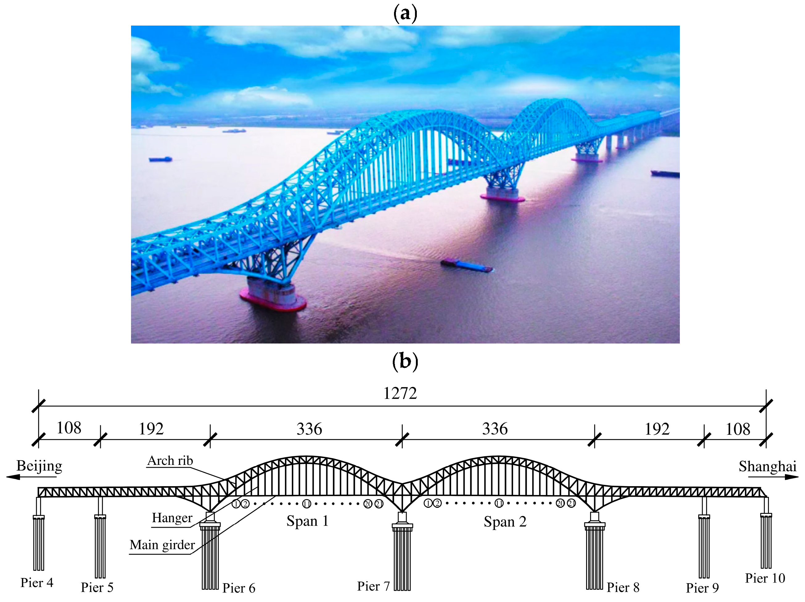
The Dashengguan Bridge is a long-span high-speed railway steel bridge crossing over Yangtze River in Nanjing, China. Figure 2a show an actual image of this bridge. The construction of this structure began in 2006 and ended in 2010 to handle a speed of 300 km/h. The bridge consists of a large-span continuous steel arch truss with a total length of 1615 m. This research considers the six main parts of the bridge with the total length of 1272 m (i.e., 108, 192, 336, 336, 192, and 108 m), as depicted in Figure 2b. These parts are separated by seven piers (Piers 4–10) mounted on deep piles. The two main spans over the major navigation channels of the Yangtze River are steel arch trusses with the lengths of 336 m and a maximum height of 74 m. The non-curved parts of the bridge have a constant height of 16 m [45]. The arches are comprised of three truss planes above the deck. The main truss has a welded, monolithic joint. The members and gusset plates were welded together in the fabrication yard and then transported to the site and spliced outside the joint with high-strength bolts.
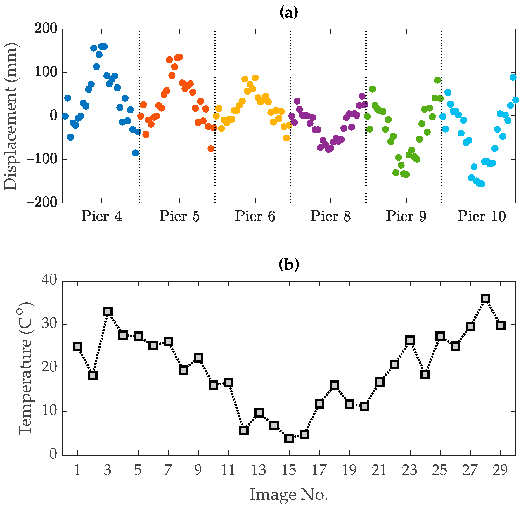
To analyze the longitudinal displacement of the bridge and investigate the effect of temperature variability, this paper utilizes the displacement samples extracted from 29 SAR images of Sentinel-1A acquired between 25 April 2015 and 5 August 2016. These displacement points were obtained by Huang et al. [45] using the persistent scatterer interferometry (PSI) technique and determining the light of sight (LOS) deformation time series at the six piers (i.e., Piers 4–6 and 8–10). Moreover, some contact-based temperature sensors were installed in the bridge to record temperature data during the monitoring time. Figure 3a shows the 29 displacement samples (i.e., in the unit of mm) at the six piers, and Figure 3b indicates their corresponding air temperature (°C).
The process of input–output data normalization begins by training the GPR and SVR models, for which the recorded temperature and limited displacement sets are used as the input (predictor) and output (response) data, respectively. Bayesian hyperparameter optimization is utilized to optimize some hyperparameters of the GPR and SVR models, as listed in Table 1 and Table 2, respectively. Note that the ratios of 80% and 20% are considered for the training and testing sets. Once the GPR and SVR models have been trained, the residual function E = Y Y ^ is employed to extract the normalized displacement data, where Y ^ denotes the predicted displacement data from the supervised regression models.
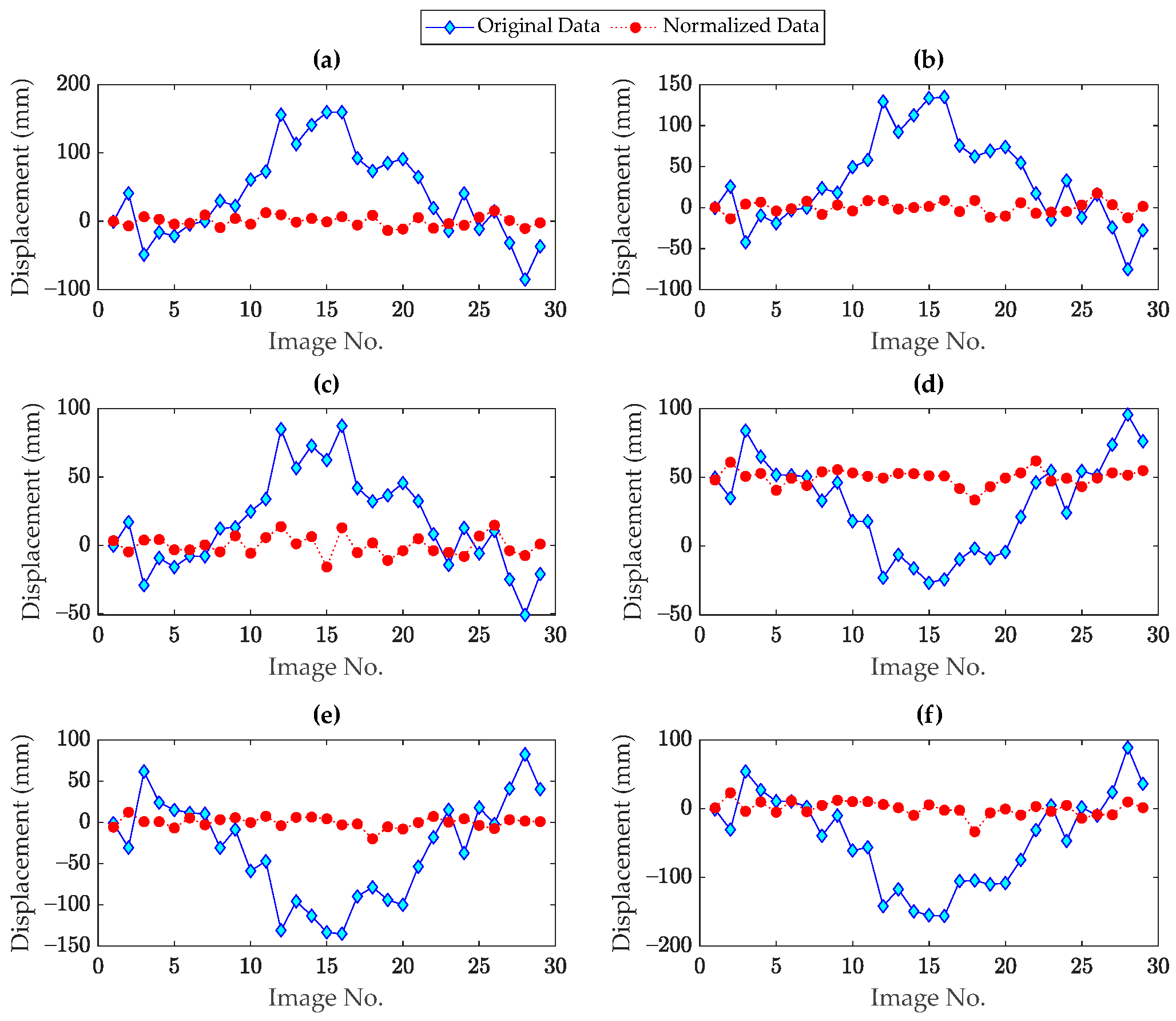
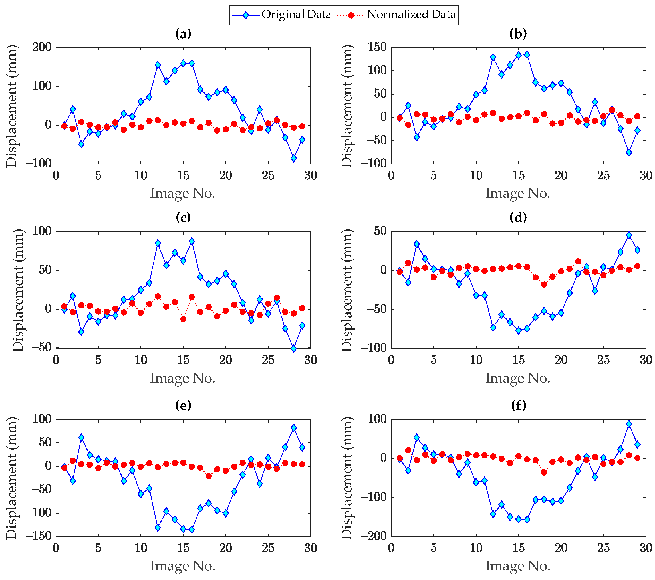
 Figure 4 and Figure 5 show the results of the thermal effect elimination by comparing the original and normalized displacement data at the six piers. As can be seen, the normalized displacement samples differ from the original ones, and most of them vary in the vicinity of the baseline with the displacement rate equal to zero [20]. This means that the normalized displacements have been separated from the thermal effects.
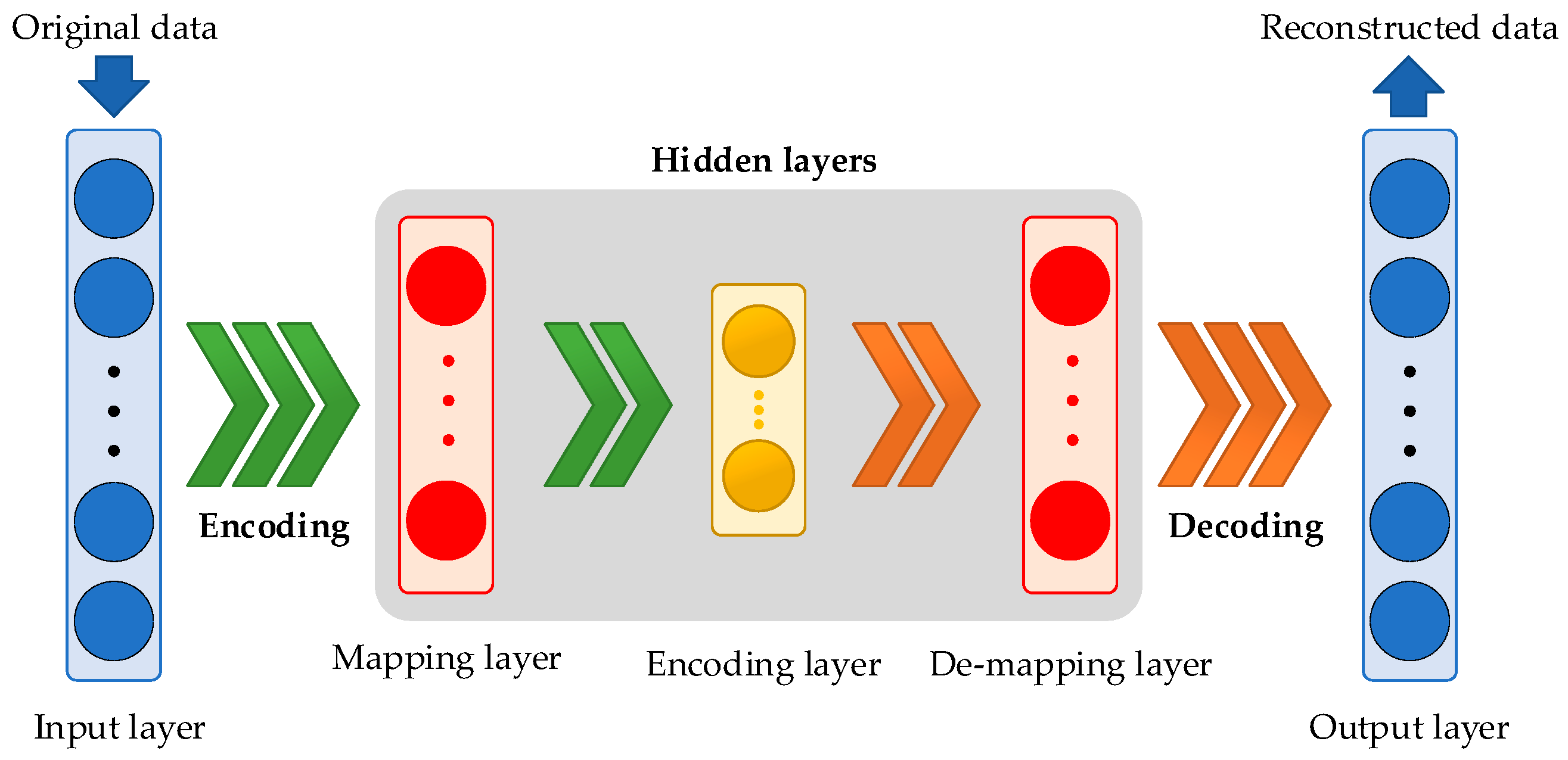
Subsequently, the unsupervised reconstruction-based data normalization techniques based on the PCA and DAE are used to eliminate the temperature influences and other unmeasured environmental and/or operational conditions. The initial requirements for these techniques are their hyperparameters. By collecting the displacement samples of the six piers into a matrix with a size of 29 × 6, the optimal number of PCs with the threshold equal to 0.9 is identical to 1. On the other hand, to determine the hyperparameters of the DAE (i.e., the neuron numbers of the mapping/de-mapping layers lm and encoding layer lc), the grid search algorithm initially utilizes two different sets of sample neurons, which are equal to 1:20 for the mapping/de-mapping layers and 1:10 for the encoding layer. Note that as the proposed DAE has a symmetric configuration, the neuron numbers of the mapping and de-mapping layers are identical. In this regard, one needs to train a DAE by using each of the sample neurons, compute the RMSE value as expressed in Equation (31), and store the computed value in a matrix. 
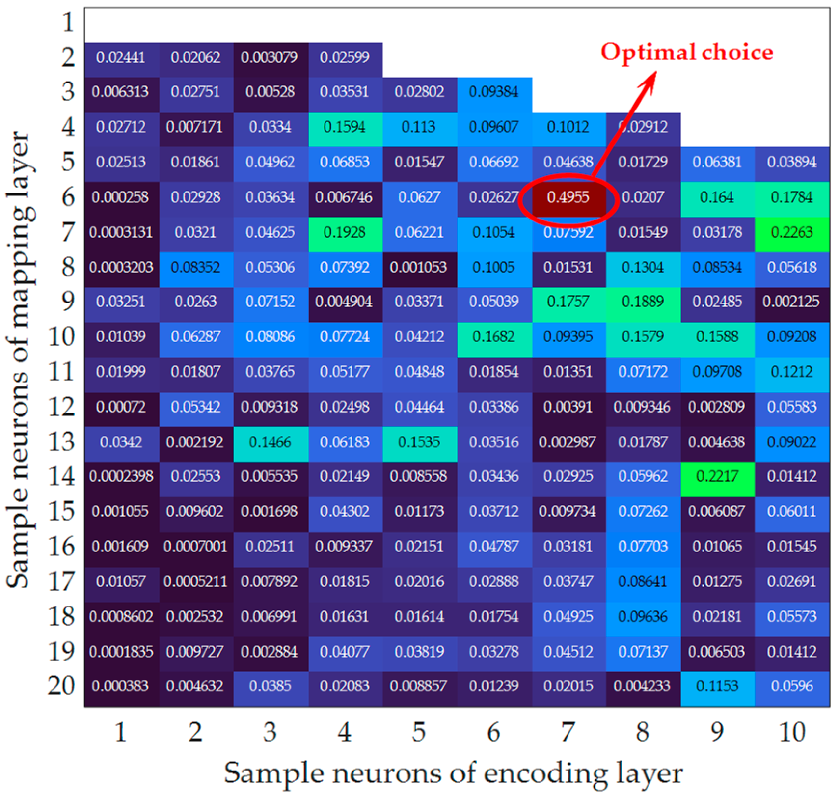
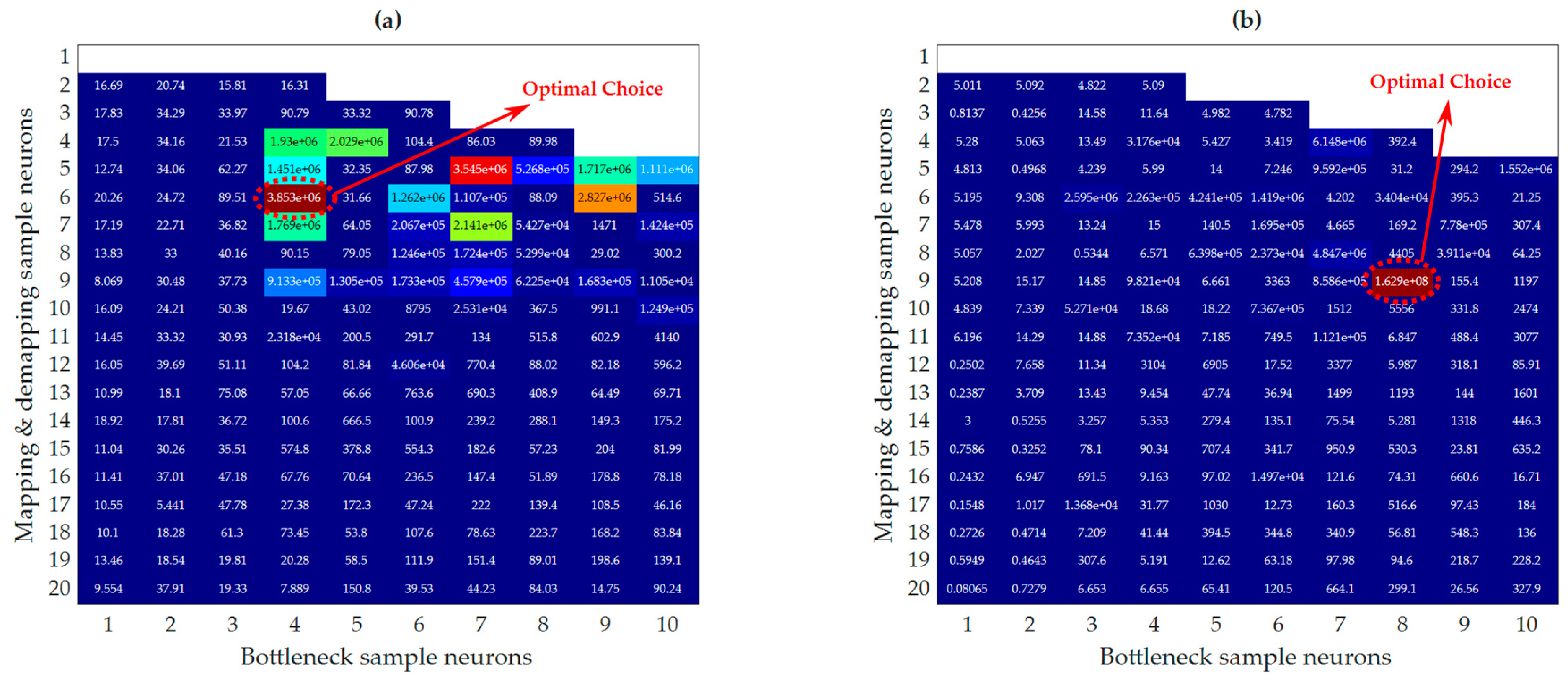
Figure 6 illustrates the inverse of the stored RMSE values of the sample neurons, which have been stored in a matrix with 20 rows and 10 columns. Notice that the inverted RMSE is applied to better indicate the result. On this basis, the optimal numbers of lm and lc coincide with the sample neurons with the largest value of the inverted RMSE quantities. With this description, it can be found that the optimal neuron sizes correspond to lm = 6 and lc = 7. Hence, a DAE with 6, 7, and 6 neurons for the mapping, encoding, and de-mapping layers is trained to reconstruct the original (multivariate) displacement data. Once the reconstructed (predicted) displacement data have been determined using the PCA and DAE models, the residual function E = Y Y ^ is used to extract the normalized displacement data.
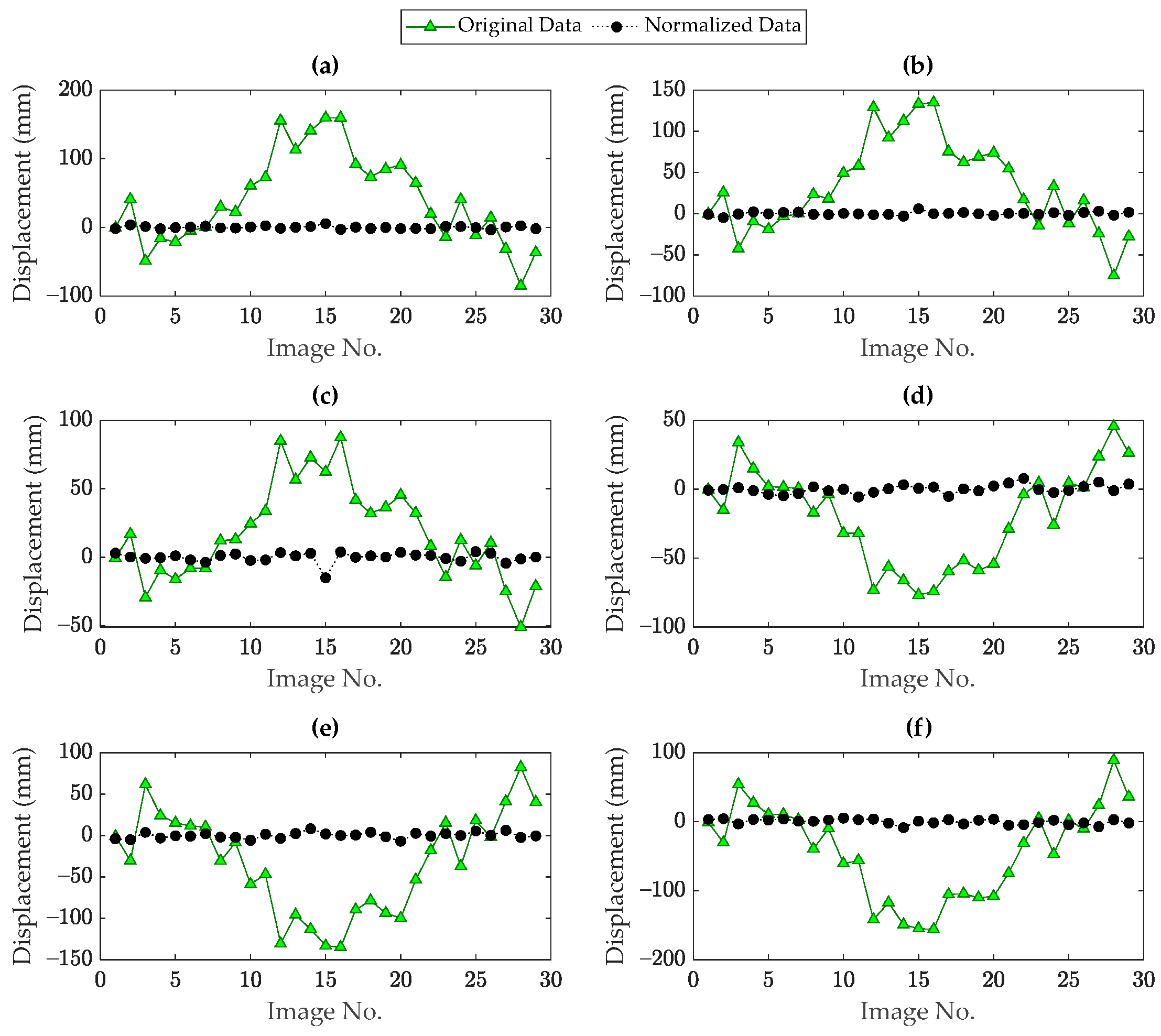
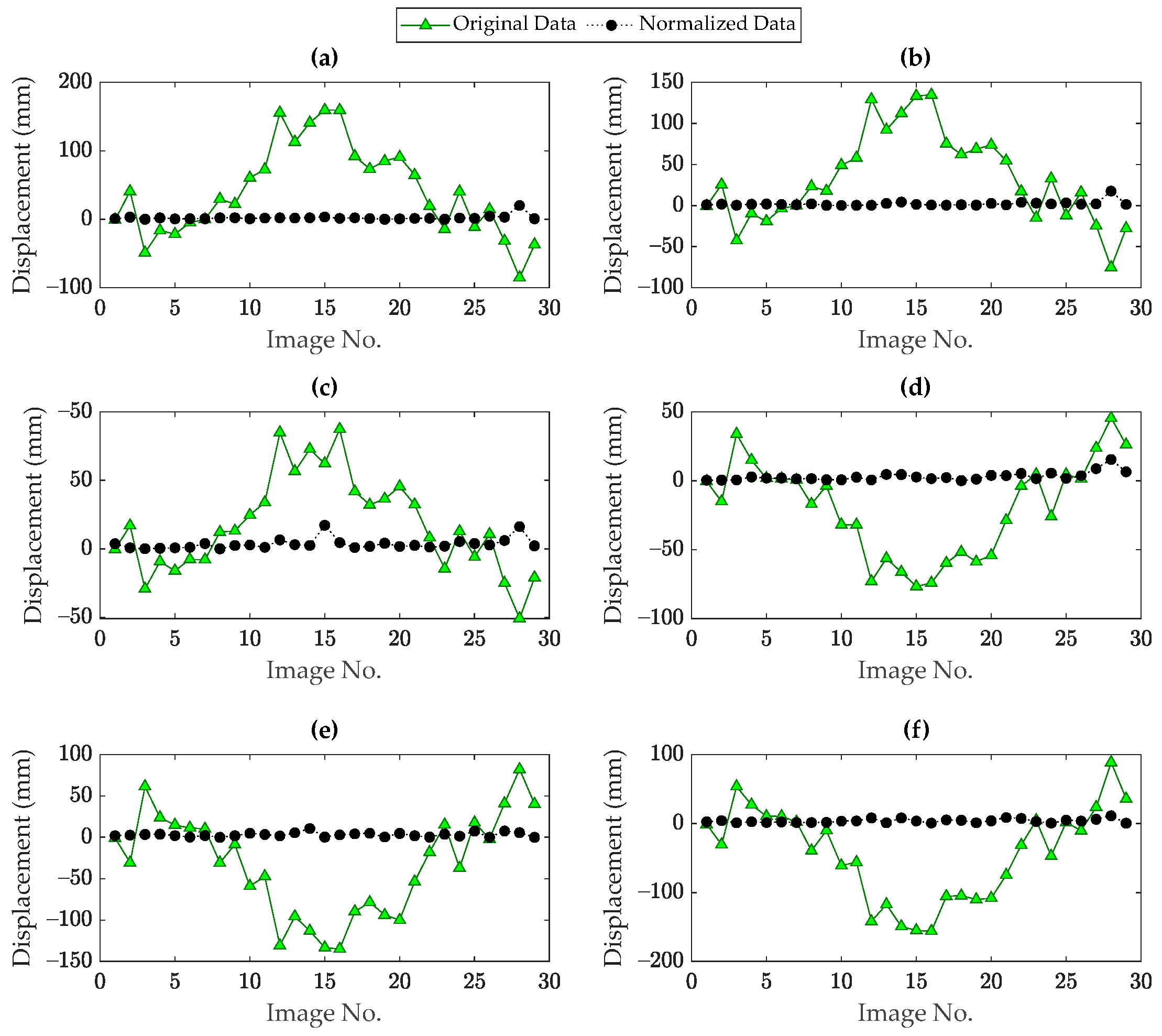
Figure 7 and Figure 8 show the results of output-only data normalization based on the PCA and DAE methods, respectively. Similar to the supervised regression models, one can perceive that the normalized displacement data differ from the original data. Approximately, all normalized points coincide with the baseline, which demonstrates the appropriate separation of the displacement data from the thermal effects. This conclusion not only verifies the effectiveness of the unsupervised data normalization methods in removing the thermal effects but also indicates their great ability to implement the process of data normalization without measuring the temperature data. Finally, to show the quality of the normalized responses and also the performance of the supervised and unsupervised data normalization models, Table 3 lists the R-squared values at the six piers of the Dashengguan Bridge. As can be observed, all quantities are close to one, which means that not only the data normalization models could predict the displacement responses properly but also the normalized responses are extracted correctly.
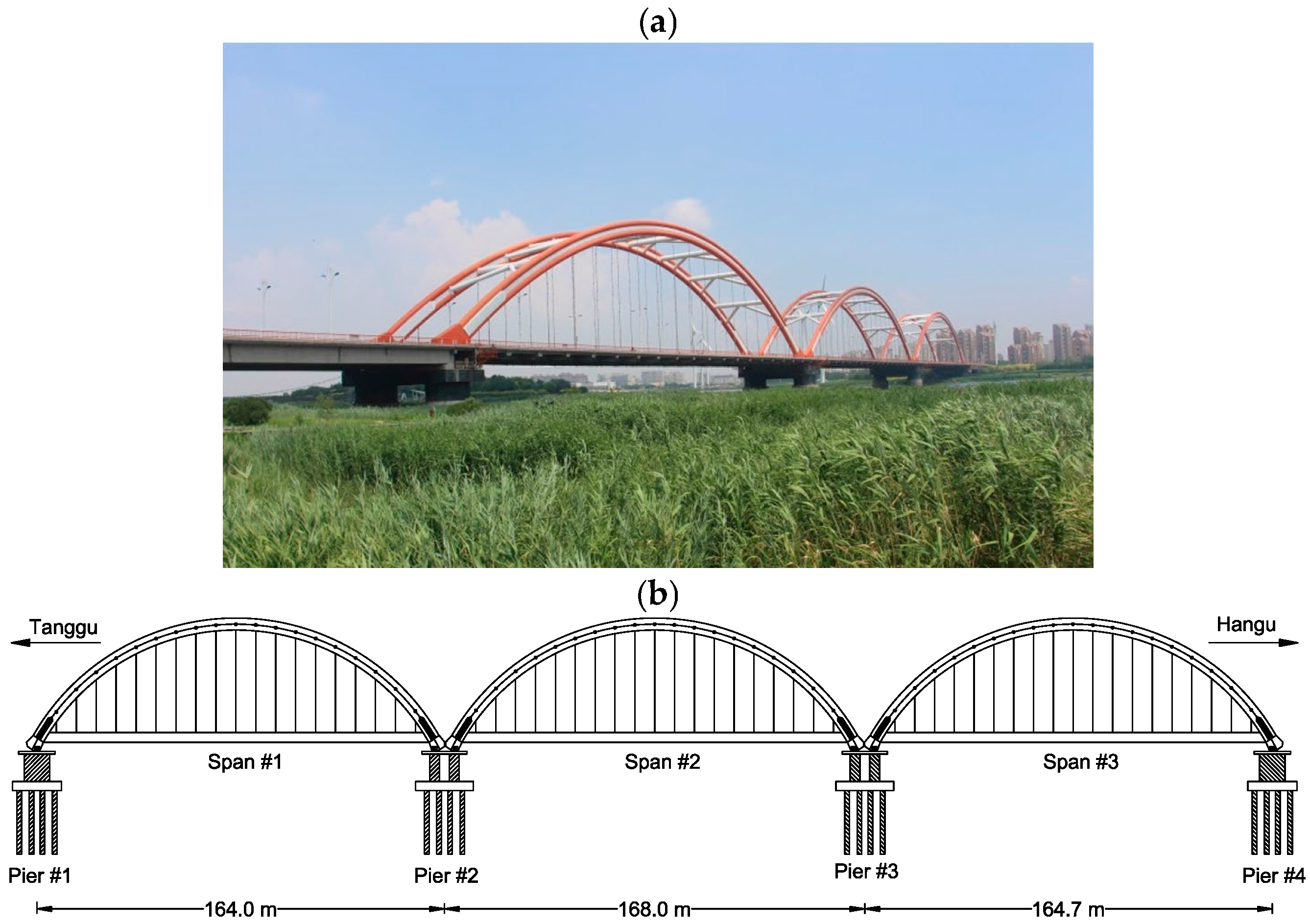
5.2. Rainbow Bridge

The Rainbow Bridge is a long-span structure in Tianjin, China that was designed and constructed as a concrete-filled steel tubular arch bridge. This structure was built in 1996 and then opened to traffic at the end of 1998. Figure 9a shows an actual image of the Rainbow Bridge. The total length of this bridge corresponds to 1215.69 m, while the main bridge structure contains three spans with the lengths of 164, 168, and 164.7 m as shown in Figure 9b. The bridge structure includes a rigid arch system with a simple supported down-bearing flexible tie rod. The upper and lower chords, along with the arch skewback, were filled with micro-expansive concrete. There are eight K-shaped transverse bracings for each span. Each arch contains 18 pairs of suspenders with a spacing of 8.3 m, and each suspender is composed of 91 galvanized prestressed steel wires. The deck system consists of a prestressed concrete middle cross girder, reinforced concrete T-shaped stiffened longitudinal girder, and T-shaped longitudinal girder [62].
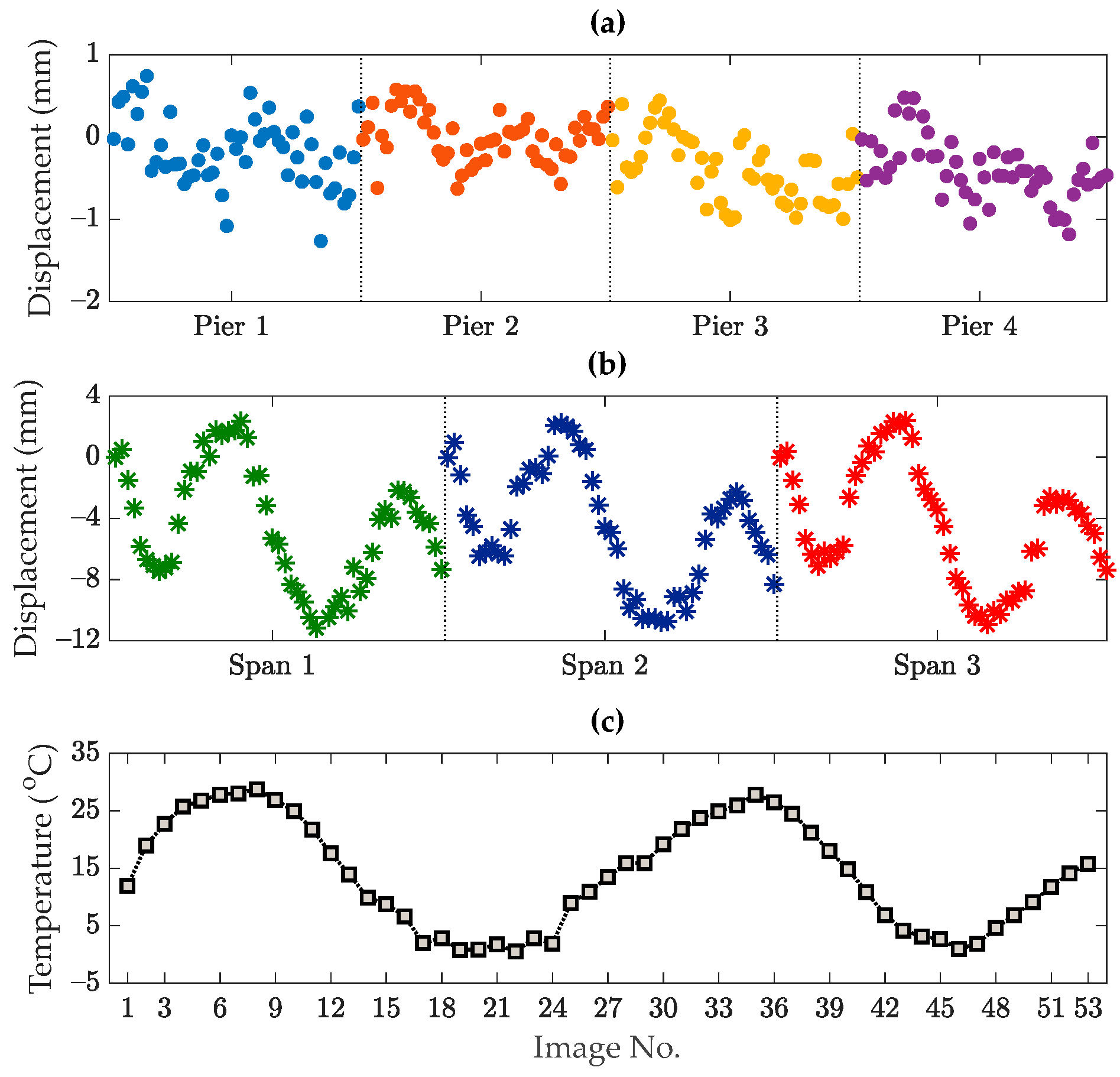
Due to the long-term passage of overweight vehicles exceeding the design load, serious damage patterns influenced the performance and serviceability of the Rainbow Bridge. In this regard, some cracks were detected at a longitudinal concrete beam of the bridge, which caused varying levels of damage in two adjacent longitudinal concrete beams. To avoid any catastrophic events, such as failure and collapse, all longitudinal concrete beams were replaced to increase the bridge structural performance. To evaluate the integrity of the bridge, long-term SAR-based SHM was implemented by Qin et al. [46] using 53 descending SAR images from Sentinel-1A between 2015 and 2017. Using a multi-temporal differential synthetic aperture radar interferometry (DInSAR) technique, Figure 10a,b illustrates the displacement samples in the main four piers (i.e., Piers 1–4) and middle spans (i.e., Span 1–3), respectively. Moreover, Figure 10c displays the temperature records during the monitoring time.
Using the temperature and displacement data, both of them are divided into the training and testing sets based on the ratios of 80% and 20%, respectively, to prepare the predictor (input) and response (output) data for the GPR and SVR models. Bayesian hyperparameter optimization is employed to optimize the main hyperparameters, as listed in Table 4 and Table 5. Based on these hyperparameters, the supervised regression models are trained to predict the displacement data and then extract the normalized data. 
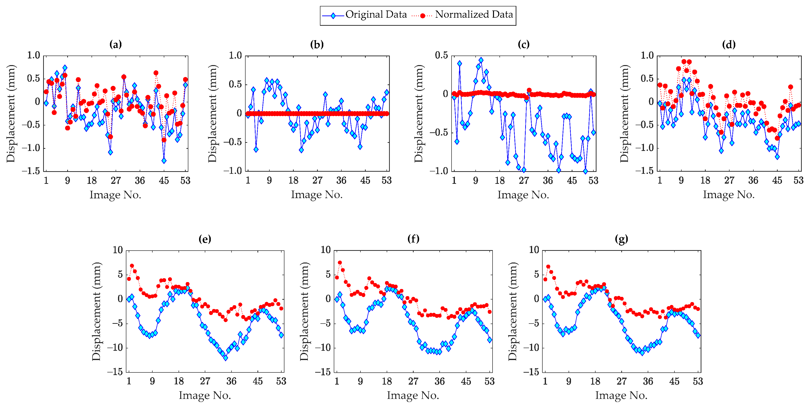
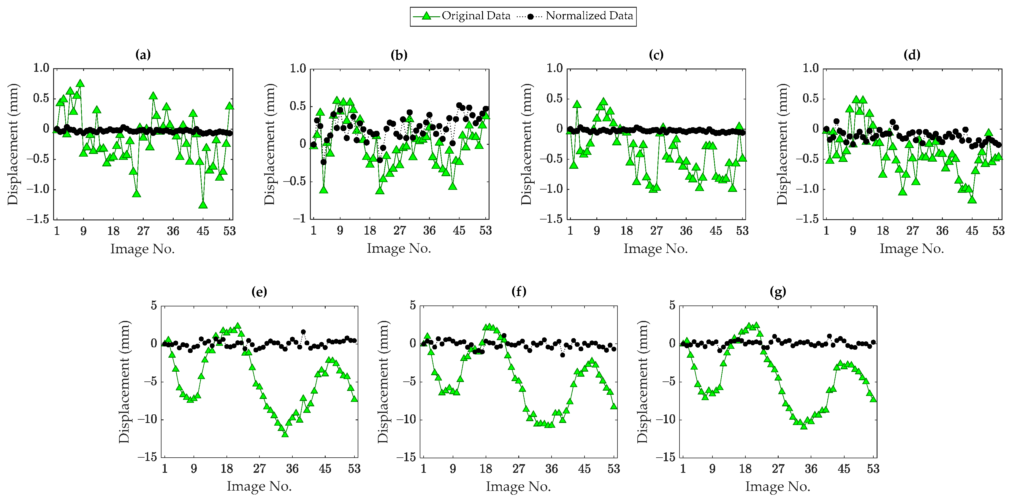
Figure 11 compares the original and normalized displacement data points of the four piers and three spans regarding the process of data normalization via the GPR. Apart from the results associated with the second and third piers, as shown in Figure 11b,c, the other plots demonstrate that this supervised regression technique could not present reliable normalized displacement data. As can be observed, the normalized samples of the first and fourth piers, as well as all three spans, conform with the original data. This means that the normalized displacement data of these locations are still influenced by the temperature variability and the GPR techniques could not be successful in data normalization.
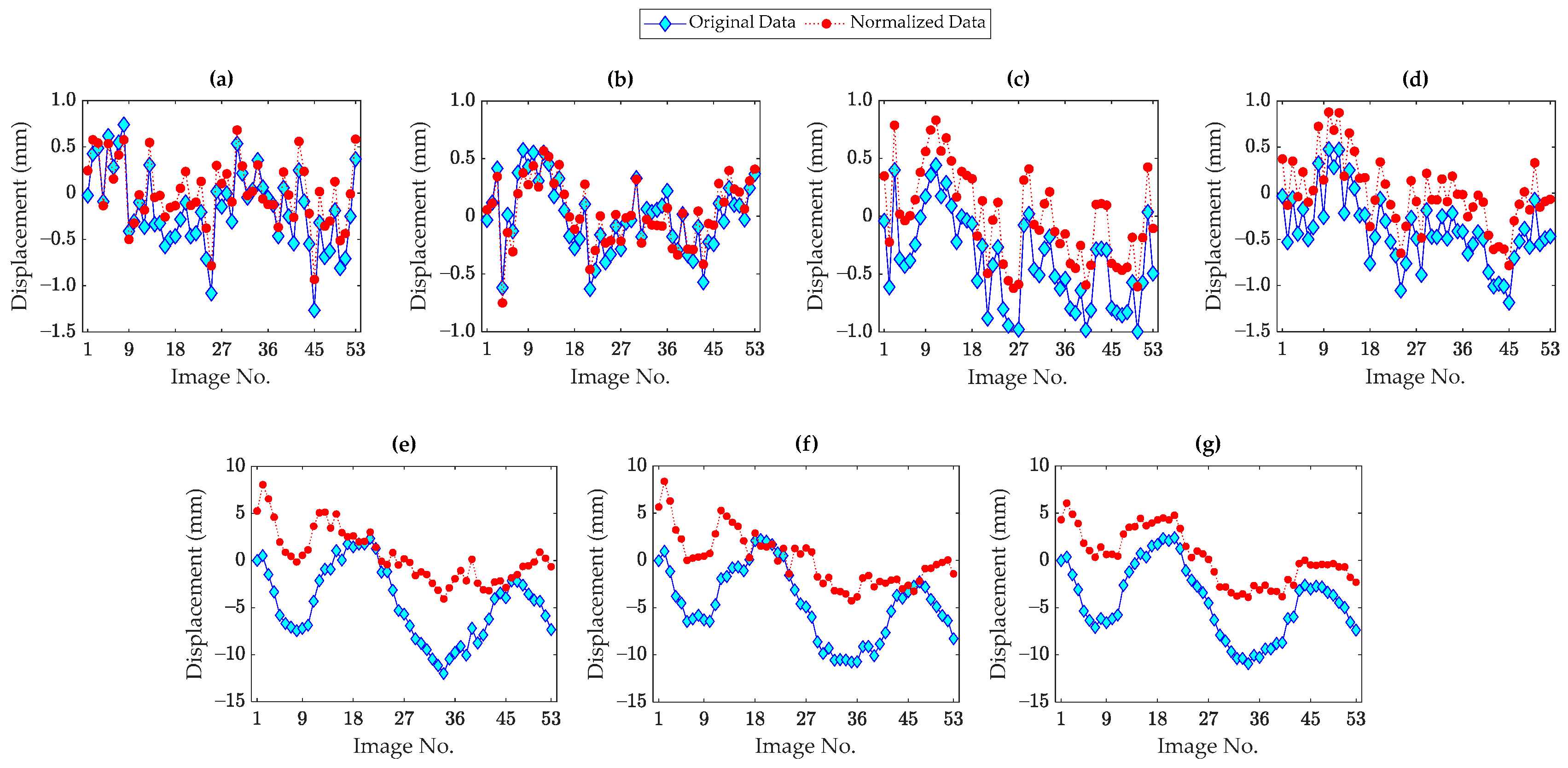
The results of data normalization through the SVR technique are displayed in Figure 12. As can be seen, this technique underperforms compared to the GPR. In all piers and spans, the normalized displacement data obtained from the SVR have the same forms as the original data. Accordingly, one can conclude that both supervised regression models failed in eliminating the temperature variability from the displacement data. Thus, the results verify that the use of temperature data as the input cannot be sufficiently effective for modeling influential supervised regression models and establishing the relationship between the displacement and temperature data. In other words, an unmeasured environmental and/or operational condition affected the displacement data of the Rainbow Bridge. Since this unmeasured condition was not included in training the GPR and SVR models, both of them could not yield reasonable outputs.
In order to investigate the environmental and/or operational effects on the limited displacement data via unsupervised data normalization techniques, the displacement samples are collected to make four multivariate datasets (matrices) regarding the piers and spans of the Rainbow Bridge. Using these matrices, the hyperparameter optimization of the PCA is carried out to choose the number of principal components with the threshold value equal to 0.9. According to the indicator IPC in Equation (26), only one PC is required to model the PCA. Hence, once the PCA model for each multivariate dataset has been established, its residual function is considered to extract the normalized displacement data. In this regard, 
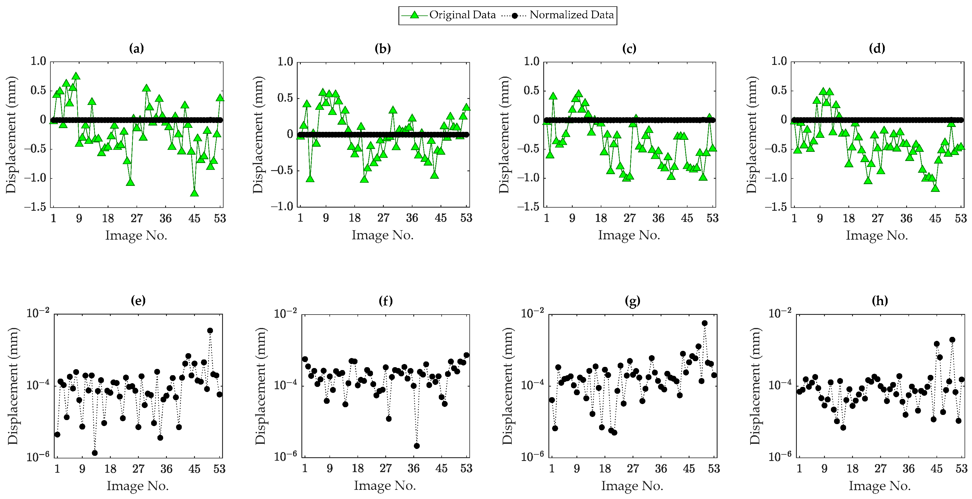
Figure 13 shows the original and normalized displacement samples regarding the unsupervised data normalization via the PCA technique. From Figure 13b, one can understand that the PCA model of the second pier could not properly extract the normalized data as it follows the same form of the original data. However, the other PCA models related to the first, third, and fourth piers, as shown in Figure 13a,c,d, have been developed accurately, in which case their normalized points approximately coincide with the baselines. Regarding the three spans, as Figure 13e,f reveals, all PCA models could properly remove the thermal and other environmental/operational effects from the displacement data.
To perform the unsupervised data normalization via the DAE, it is necessary to determine the neuron sizes of the mapping, encoding, and de-mapping layers. Utilizing the same sample neurons of the preceding structure, which are equal to 1:20 for the mapping/de-mapping layers and 1:10 for the encoding layer, Figure 14 illustrates the inverted RMSE values regarding the four piers and three spans of the Rainbow Bridge. Among the aforementioned sample neurons used in the grid search algorithm, the best DAE for modeling the displacement data of the piers requires 6 and 4 neurons for the mapping (de-mapping) and encoding layers, respectively, as these neurons provide the maximum inverted RMSE values, which are equivalent to the minimum RMSE values.
Furthermore, the optimal numbers of lm and lc regarding the DAE of the displacement samples of the three spans are equal to 9 and 8, respectively. It should be emphasized that we applied the inverted RMSE to better indicate the result of hyperparameter optimization. The results of the DAE-based data normalization at the piers and spans of the Rainbow Bridge are shown in
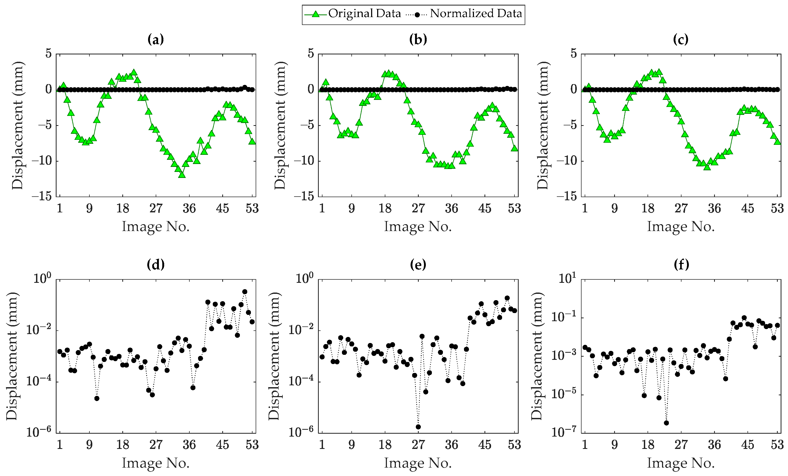
 Figure 15 and Figure 16, respectively. To better show the results, the normalized displacement samples are separately plotted in Figure 15e–h and Figure 16d–f. In contrast to all the previous techniques, the DAE yielded the best performance in removing the thermal effects. As can be observed, all normalized displacement samples coincide with the baselines, which means that the DAE-based data normalization method could thoroughly eliminate the thermal or other environmental/operational effects.
To demonstrate the quality of the normalized responses and also assess the performance of the supervised and unsupervised data normalization models, Table 6 presents their R-squared values at the piers and spans of the Rainbow Bridge. As can be discerned, the DAE-aided data normalization method provides the most reliable normalized responses because all R-squared values roughly correspond to one. In relation to the normalized responses of the four piers, the worst performance belongs to the SVR model since all R-squared quantities are far away from one. The GPR model also failed in extracting reliable normalized responses for the first and fourth piers. The PCA model is approximately successful; however, the normalized response of the second pier is not reasonable. Regarding the spans of the Rainbow Bridge, one can observe that the R-squared values of the supervised predictive models yielded moderate R-squared values varying within 0.45–0.55, which implies that the normalized responses could not be extracted appropriately. However, both the PCA and DAE methods could attain the best performances for extracting the normalized responses of the bridge spans.

6. Conclusions

This paper conducted a practical and comprehensive investigation into the effects of temperature variability on limited displacement data retrieved from a small number of SAR images based on the technology of remote sensing with the aid of contact-based temperature sensors related to the supervised data normalization algorithms and without such sensors concerning the unsupervised data normalization methods. The main objective was to eliminate the thermal effects from displacement data by using and comparing different machine learning-aided data normalization techniques. Hence, the supervised regression models based on the GPR and SVR were initially employed to perform the input–output data normalization. Subsequently, the process continued by using the unsupervised reconstruction-based techniques developed from the PCA and DAE. The limited displacement samples of two long-span bridges from a few SAR images of Sentinel-1A were used to evaluate the performances of the above-mentioned data normalization techniques. The main results of this work can be summarized as follows:
i
The input–output (supervised) data normalization techniques can perform well provided that the temperature is the main variability factor. When the other environmental and/or operational conditions influence the structure and these are not included in the supervised regression modeling, the input–output data normalization techniques fail in eliminating the variability sources. Under such circumstances, the residuals or normalized responses obtained from such techniques still contain the environmental and/or operational conditions leading to similarities in the forms of the original and normalized responses.
ii
Due to the importance of the input data in learning or developing input–output supervised models, it is essential to measure all possible environmental (e.g., humidity, wind speed and direction, etc.) and operational (e.g., traffic loads and volumes, live loads, etc.) conditions. When the measurements of such environmental and operational variability are not feasible, the best choice is to apply output-only (unsupervised) data normalization methods.
iii
In contrast to the input–output data normalization techniques, both the PCA and DAE models succeeded in accurately removing the thermal and other unmeasured variability conditions.
iv
In all cases of the influences of variability conditions and based on the R-squared values, especially in the problem of the Rainbow Bridge, the DAE-based data normalization yielded the best performance. Hence, it is preferred to apply this method to remove the environmental variability.
v
The findings of this research are suitable for long-term health monitoring of large-scale civil structures, particularly long-span bridges, with the aid of the remote sensing technology and providing normalized displacement responses insensitive to environmental and/or operational variability. However, it should be noted that a data normalization technique may be successful in removing a specific type of variability condition, but it might also hide changes due to damage, a sudden and critical event caused by an earthquake, and gradual variations due to a slow landslide or ageing. Hence, it is essential to evaluate the output of any data normalization technique based on a residual analysis based on some metrics, such as the R-squared statistic, and control charts for assessing anomalies in residual samples.
For future research activities, it is recommended to explore the process of the removal of environmental and/or operational variability from limited displacement responses extracted from SAR images by proposing new input–output (supervised) and output-only (unsupervised) data normalization methods under advanced machine learning algorithms. These algorithms include but are not limited to ensemble learning, hybrid learning, incremental learning, and teacher–student learning. Moreover, based on the first conclusion, it is suggested to develop a new input–output data normalization framework by initially analyzing the correlation between the input (the measured environmental factor) and output (displacement) data and then selecting an appropriate regression model.

Author Contributions

Conceptualization, B.B., A.E. and C.D.M.; methodology, B.B., A.E. and C.D.M.; software, B.B. and A.E.; validation, B.B. and A.E.; formal analysis, B.B., A.E., C.D.M. and A.N.A.; investigation, B.B., A.E., C.D.M. and A.N.A.; resources, B.B. and A.E.; data curation, B.B. and A.E.; writing—original draft preparation, B.B. and A.E.; writing—review and editing, B.B., A.E., C.D.M. and A.N.A.; visualization, B.B., A.E., C.D.M. and A.N.A.; supervision, C.D.M. and A.N.A.; project administration, B.B., A.E., C.D.M. and A.N.A. All authors have read and agreed to the published version of the manuscript.

Funding

This research was partially funded by the European Space Agency (ESA) under ESA contract no. 4000132658/20/NL/MH/ac.

Data Availability Statement

Data is unavailable due to privacy or ethical restrictions.

Conflicts of Interest

The authors declare no conflict of interest.

References

  1. Su, J.; Xia, Y.; Weng, S. Review on field monitoring of high-rise structures. Struct. Contr. Health Monit. 2020, 27, e2629. [Google Scholar] [CrossRef]
  2. Scaioni, M.; Marsella, M.; Crosetto, M.; Tornatore, V.; Wang, J. Geodetic and Remote-Sensing Sensors for Dam Deformation Monitoring. Sensors 2018, 18, 3682. [Google Scholar] [CrossRef] [PubMed] [Green Version]
  3. Ahmed, H.; La, H.M.; Gucunski, N. Review of Non-Destructive Civil Infrastructure Evaluation for Bridges: State-of-the-Art Robotic Platforms, Sensors and Algorithms. Sensors 2020, 20, 3954. [Google Scholar] [CrossRef] [PubMed]
  4. Chen, Q.; Jiang, W.; Meng, X.; Jiang, P.; Wang, K.; Xie, Y.; Ye, J. Vertical Deformation Monitoring of the Suspension Bridge Tower Using GNSS: A Case Study of the Forth Road Bridge in the UK. Remote Sens. 2018, 10, 364. [Google Scholar] [CrossRef] [Green Version]
  5. Gonen, S.; Erduran, E. A Hybrid Method for Vibration-Based Bridge Damage Detection. Remote Sens. 2022, 14, 6054. [Google Scholar] [CrossRef]
  6. Shen, N.; Chen, L.; Liu, J.; Wang, L.; Tao, T.; Wu, D.; Chen, R. A Review of Global Navigation Satellite System (GNSS)-Based Dynamic Monitoring Technologies for Structural Health Monitoring. Remote Sens. 2019, 11, 1001. [Google Scholar] [CrossRef] [Green Version]
  7. Pepe, A.; Calò, F. A Review of Interferometric Synthetic Aperture RADAR (InSAR) Multi-Track Approaches for the Retrieval of Earth’s Surface Displacements. Appl. Sci. 2017, 7, 1264. [Google Scholar] [CrossRef] [Green Version]
  8. Biondi, F.; Addabbo, P.; Ullo, S.L.; Clemente, C.; Orlando, D. Perspectives on the Structural Health Monitoring of Bridges by Synthetic Aperture Radar. Remote Sens. 2020, 12, 3852. [Google Scholar] [CrossRef]
  9. Daneshvar, M.H.; Sarmadi, H. Unsupervised learning-based damage assessment of full-scale civil structures under long-term and short-term monitoring. Eng. Struct. 2022, 256, 114059. [Google Scholar] [CrossRef]
  10. Yang, H.; Xu, H.-C.; Jiao, S.-J.; Yin, F.-D. Semantic Image Segmentation Based Cable Vibration Frequency Visual Monitoring Using Modified Convolutional Neural Network with Pixel-wise Weighting Strategy. Remote Sens. 2021, 13, 1466. [Google Scholar] [CrossRef]
  11. Gardner, P.; Liu, X.; Worden, K. On the application of domain adaptation in structural health monitoring. Mech. Syst. Sig. Process. 2020, 138, 106550. [Google Scholar] [CrossRef]
  12. Sarmadi, H.; Yuen, K.-V. Early damage detection by an innovative unsupervised learning method based on kernel null space and peak-over-threshold. Comput. Aided Civ. Inf. 2021, 36, 1150–1167. [Google Scholar] [CrossRef]
  13. Sarmadi, H.; Entezami, A.; Saeedi Razavi, B.; Yuen, K.-V. Ensemble learning-based structural health monitoring by Mahalanobis distance metrics. Struct. Contr. Health Monit. 2021, 28, e2663. [Google Scholar] [CrossRef]
  14. Entezami, A.; Shariatmadar, H.; De Michele, C. Non-parametric empirical machine learning for short-term and long-term structural health monitoring. Struct. Health Monit. 2022, 21, 2700–2718. [Google Scholar] [CrossRef]
  15. Entezami, A.; Sarmadi, H.; Behkamal, B. Long-term health monitoring of concrete and steel bridges under large and missing data by unsupervised meta learning. Eng. Struct. 2023, 279, 115616. [Google Scholar] [CrossRef]
  16. Entezami, A.; Sarmadi, H.; Behkamal, B.; De Michele, C. On continuous health monitoring of bridges under serious environmental variability by an innovative multi-task unsupervised learning method. Struct. Infrastruct. Eng. 2023, 1–19. [Google Scholar] [CrossRef]
  17. Sarmadi, H.; Karamodin, A. A novel anomaly detection method based on adaptive Mahalanobis-squared distance and one-class kNN rule for structural health monitoring under environmental effects. Mech. Syst. Sig. Process. 2020, 140, 106495. [Google Scholar] [CrossRef]
  18. Entezami, A.; Arslan, A.N.; De Michele, C.; Behkamal, B. Online hybrid learning methods for real-time structural health monitoring using remote sensing and small displacement data. Remote Sens. 2022, 14, 3357. [Google Scholar] [CrossRef]
  19. Entezami, A.; De Michele, C.; Arslan, A.N.; Behkamal, B. Detection of partially structural collapse using long-term small displacement data from satellite images. Sensors 2022, 22, 4964. [Google Scholar] [CrossRef]
  20. Xu, X.; Huang, Q.; Ren, Y.; Zhao, D.-Y.; Yang, J.; Zhang, D.-Y. Modeling and Separation of Thermal Effects from Cable-Stayed Bridge Response. J. Bridge Eng. 2019, 24, 04019028. [Google Scholar] [CrossRef]
  21. Sarmadi, H.; Yuen, K.-V. Structural health monitoring by a novel probabilistic machine learning method based on extreme value theory and mixture quantile modeling. Mech. Syst. Sig. Process. 2022, 173, 109049. [Google Scholar] [CrossRef]
  22. Kita, A.; Cavalagli, N.; Ubertini, F. Temperature effects on static and dynamic behavior of Consoli Palace in Gubbio, Italy. Mech. Syst. Sig. Process. 2019, 120, 180–202. [Google Scholar] [CrossRef]
  23. Wang, Z.; Yang, D.-H.; Yi, T.-H.; Zhang, G.-H.; Han, J.-G. Eliminating environmental and operational effects on structural modal frequency: A comprehensive review. Struct. Contr. Health Monit. 2022, 29, e3073. [Google Scholar] [CrossRef]
  24. Farreras-Alcover, I.; Chryssanthopoulos, M.K.; Andersen, J.E. Regression models for structural health monitoring of welded bridge joints based on temperature, traffic and strain measurements. Struct. Health Monit. 2015, 14, 648–662. [Google Scholar] [CrossRef] [Green Version]
  25. Roberts, C.; Cava, D.G.; Avendaño-Valencia, L.D. Addressing practicalities in multivariate nonlinear regression for mitigating environmental and operational variations. Struct. Health Monit. 2022, 22, 1237–1255. [Google Scholar] [CrossRef]
  26. Laory, I.; Trinh, T.N.; Smith, I.F.C.; Brownjohn, J.M.W. Methodologies for predicting natural frequency variation of a suspension bridge. Eng. Struct. 2014, 80, 211–221. [Google Scholar] [CrossRef] [Green Version]
  27. Jang, J.; Smyth, A.W. Data-driven models for temperature distribution effects on natural frequencies and thermal prestress modeling. Struct. Contr. Health Monit. 2020, 27, e2489. [Google Scholar] [CrossRef]
  28. Ma, K.-C.; Yi, T.-H.; Yang, D.-H.; Li, H.-N.; Liu, H. Nonlinear Uncertainty Modeling between Bridge Frequencies and Multiple Environmental Factors Based on Monitoring Data. J. Perform. Constr. Facil. 2021, 35, 04021056. [Google Scholar] [CrossRef]
  29. Ni, Y.Q.; Zhou, H.F.; Ko, J.M. Generalization Capability of Neural Network Models for Temperature-Frequency Correlation Using Monitoring Data. J. Struct. Eng. 2009, 135, 1290–1300. [Google Scholar] [CrossRef]
  30. Coletta, G.; Miraglia, G.; Pecorelli, M.; Ceravolo, R.; Cross, E.; Surace, C.; Worden, K. Use of the cointegration strategies to remove environmental effects from data acquired on historical buildings. Eng. Struct. 2019, 183, 1014–1026. [Google Scholar] [CrossRef]
  31. Qin, Y.; Li, Y.; Liu, G. Separation of the Temperature Effect on Structure Responses via LSTM-Particle Filter Method Considering Outlier from Remote Cloud Platforms. Remote Sens. 2022, 14, 4629. [Google Scholar] [CrossRef]
  32. Yan, A.-M.; Kerschen, G.; De Boe, P.; Golinval, J.-C. Structural damage diagnosis under varying environmental conditions—Part II: Local PCA for non-linear cases. Mech. Syst. Sig. Process. 2005, 19, 865–880. [Google Scholar] [CrossRef]
  33. Reynders, E.; Wursten, G.; De Roeck, G. Output-only structural health monitoring in changing environmental conditions by means of nonlinear system identification. Struct. Health Monit. 2014, 13, 82–93. [Google Scholar] [CrossRef]
  34. Comanducci, G.; Magalhães, F.; Ubertini, F.; Cunha, Á. On vibration-based damage detection by multivariate statistical techniques: Application to a long-span arch bridge. Struct. Health Monit. 2016, 15, 505–524. [Google Scholar] [CrossRef]
  35. Figueiredo, E.; Park, G.; Farrar, C.R.; Worden, K.; Figueiras, J. Machine learning algorithms for damage detection under operational and environmental variability. Struct. Health Monit. 2011, 10, 559–572. [Google Scholar] [CrossRef]
  36. Sarmadi, H. Investigation of machine learning methods for structural safety assessment under variability in data: Comparative studies and new approaches. J. Perform. Constr. Facil. 2021, 35, 04021090. [Google Scholar] [CrossRef]
  37. Daneshvar, M.H.; Sarmadi, H.; Yuen, K.-V. A locally unsupervised hybrid learning method for removing environmental effects under different measurement periods. Measurement 2023, 208, 112465. [Google Scholar] [CrossRef]
  38. Sarmadi, H.; Entezami, A.; Behkamal, B.; De Michele, C. Partially online damage detection using long-term modal data under severe environmental effects by unsupervised feature selection and local metric learning. J. Civ. Struct. Health Monit. 2022, 12, 1043–1066. [Google Scholar] [CrossRef]
  39. Sarmadi, H.; Entezami, A.; De Michele, C. Probabilistic data self-clustering based on semi-parametric extreme value theory for structural health monitoring. Mech. Syst. Sig. Process. 2023, 187, 109976. [Google Scholar] [CrossRef]
  40. Sarmadi, H.; Entezami, A.; Magalhães, F. Unsupervised data normalization for continuous dynamic monitoring by an innovative hybrid feature weighting-selection algorithm and natural nearest neighbor searching. Struct. Health Monit. 2023; in press. [Google Scholar] [CrossRef]
  41. Teng, J.; Tang, D.-H.; Hu, W.-H.; Lu, W.; Feng, Z.-W.; Ao, C.-F.; Liao, M.-H. Mechanism of the effect of temperature on frequency based on long-term monitoring of an arch bridge. Struct. Health Monit. 2021, 20, 1716–1737. [Google Scholar] [CrossRef]
  42. Yang, D.-H.; Yi, T.-H.; Li, H.-N.; Zhang, Y.-F. Monitoring and analysis of thermal effect on tower displacement in cable-stayed bridge. Measurement 2018, 115, 249–257. [Google Scholar] [CrossRef]
  43. Xia, Q.; Zhang, J.; Tian, Y.; Zhang, Y. Experimental Study of Thermal Effects on a Long-Span Suspension Bridge. J. Bridge Eng. 2017, 22, 04017034. [Google Scholar] [CrossRef]
  44. Giordano, P.; Turksezer, Z.; Previtali, M.; Limongelli, M. Damage detection on a historic iron bridge using satellite DInSAR data. Struct. Health Monit. 2022, 21, 2291–2311. [Google Scholar] [CrossRef]
  45. Huang, Q.; Crosetto, M.; Monserrat, O.; Crippa, B. Displacement monitoring and modelling of a high-speed railway bridge using C-band Sentinel-1 data. ISPRS J. Photogramm. Remote Sens. 2017, 128, 204–211. [Google Scholar] [CrossRef]
  46. Qin, X.; Zhang, L.; Yang, M.; Luo, H.; Liao, M.; Ding, X. Mapping surface deformation and thermal dilation of arch bridges by structure-driven multi-temporal DInSAR analysis. Remote Sens. Environ. 2018, 216, 71–90. [Google Scholar] [CrossRef]
  47. Farneti, E.; Cavalagli, N.; Costantini, M.; Trillo, F.; Minati, F.; Venanzi, I.; Ubertini, F. A method for structural monitoring of multispan bridges using satellite InSAR data with uncertainty quantification and its pre-collapse application to the Albiano-Magra Bridge in Italy. Struct. Health Monit. 2023, 22, 353–371. [Google Scholar] [CrossRef]
  48. Bianchini, S.; Pratesi, F.; Nolesini, T.; Casagli, N. Building Deformation Assessment by Means of Persistent Scatterer Interferometry Analysis on a Landslide-Affected Area: The Volterra (Italy) Case Study. Remote Sens. 2015, 7, 4678–4701. [Google Scholar] [CrossRef] [Green Version]
  49. Cavalagli, N.; Kita, A.; Falco, S.; Trillo, F.; Costantini, M.; Ubertini, F. Satellite radar interferometry and in-situ measurements for static monitoring of historical monuments: The case of Gubbio, Italy. Remote Sens. Environ. 2019, 235, 111453. [Google Scholar] [CrossRef]
  50. Zhu, M.; Wan, X.; Fei, B.; Qiao, Z.; Ge, C.; Minati, F.; Vecchioli, F.; Li, J.; Costantini, M. Detection of Building and Infrastructure Instabilities by Automatic Spatiotemporal Analysis of Satellite SAR Interferometry Measurements. Remote Sens. 2018, 10, 1816. [Google Scholar] [CrossRef] [Green Version]
  51. Drougkas, A.; Verstrynge, E.; Van Balen, K.; Shimoni, M.; Croonenborghs, T.; Hayen, R.; Declercq, P.-Y. Country-scale InSAR monitoring for settlement and uplift damage calculation in architectural heritage structures. Struct. Health Monit. 2021, 20, 2317–2336. [Google Scholar] [CrossRef]
  52. Yang, L.; Shami, A. On hyperparameter optimization of machine learning algorithms: Theory and practice. Neurocomputing 2020, 415, 295–316. [Google Scholar] [CrossRef]
  53. Hu, W.-H.; Cunha, Á.; Caetano, E.; Rohrmann, R.G.; Said, S.; Teng, J. Comparison of different statistical approaches for removing environmental/operational effects for massive data continuously collected from footbridges. Struct. Contr. Health Monit. 2017, 24, e1955. [Google Scholar] [CrossRef]
  54. Rasmussen, C.E.; Williams, C.K.I. Gaussian Processes for Machine Learning; MIT Press: Cambridge, MA, USA, 2005. [Google Scholar]
  55. Kung, S.Y. Kernel Methods and Machine Learning; Cambridge University Press: Cambridge, UK, 2014. [Google Scholar]
  56. Smola, A.J.; Schölkopf, B. A tutorial on support vector regression. Stat. Comput. 2004, 14, 199–222. [Google Scholar] [CrossRef] [Green Version]
  57. Deraemaeker, A.; Reynders, E.; De Roeck, G.; Kullaa, J. Vibration-based structural health monitoring using output-only measurements under changing enviroment. Mech. Syst. Sig. Process. 2008, 22, 34–56. [Google Scholar] [CrossRef] [Green Version]
  58. Deraemaeker, A.; Worden, K. A comparison of linear approaches to filter out environmental effects in structural health monitoring. Mech. Syst. Sig. Process. 2018, 105, 1–15. [Google Scholar] [CrossRef]
  59. Liu, W.; Wang, Z.; Liu, X.; Zeng, N.; Liu, Y.; Alsaadi, F.E. A survey of deep neural network architectures and their applications. Neurocomputing 2017, 234, 11–26. [Google Scholar] [CrossRef]
  60. Singh, A.; Kushwaha, S.; Alarfaj, M.; Singh, M. Comprehensive Overview of Backpropagation Algorithm for Digital Image Denoising. Electronics 2022, 11, 1590. [Google Scholar] [CrossRef]
  61. Charte, D.; Charte, F.; García, S.; del Jesus, M.J.; Herrera, F. A practical tutorial on autoencoders for nonlinear feature fusion: Taxonomy, models, software and guidelines. Inf. Fusion 2018, 44, 78–96. [Google Scholar] [CrossRef]
  62. Niu, Y.; Ye, Y.; Zhao, W.; Duan, Y.; Shu, J. Identifying Modal Parameters of a Multispan Bridge Based on High-Rate GNSS-RTK Measurement Using the CEEMD-RDT Approach. J. Bridge Eng. 2021, 26, 04021049. [Google Scholar] [CrossRef]
Figure 1. The schematic of the developed DAE (i.e., the circle refers to the neuron of each layer).
Remotesensing 15 03095 g001
Figure 2. (a) The Dashengguan Bridge; (b) the side view and main dimensions in the unit of meter.
Remotesensing 15 03095 g002
Figure 3. The Dashengguan Bridge: (a) the limited displacement data from 29 SAR images of Sentinel-1A, and (b) the temperature data from contact-based temperature sensors.
Remotesensing 15 03095 g003
Figure 4. The original and normalized displacement data based on the GPR models regarding the Dashengguan Bridge: (a) Pier 4, (b) Pier 5, (c) Pier 6, (d) Pier 8, (e) Pier 9, (f) Pier 10.
Remotesensing 15 03095 g004
Figure 5. The original and normalized displacement data based on the SVR models regarding the Dashengguan Bridge: (a) Pier 4, (b) Pier 5, (c) Pier 6, (d) Pier 8, (e) Pier 9, (f) Pier 10.
Remotesensing 15 03095 g005
Figure 6. Hyperparameter optimization of the DAE for selecting the number of neurons of hidden layers based on the inverted RMSE values (i.e., the white part refers to the NaN values).
Remotesensing 15 03095 g006
Figure 7. The original and normalized displacement data based on the PCA models regarding the Dashengguan Bridge: (a) Pier 4, (b) Pier 5, (c) Pier 6, (d) Pier 8, (e) Pier 9, (f) Pier 10.
Remotesensing 15 03095 g007
Figure 8. The original and normalized displacement data based on the DAEs regarding the Dashengguan Bridge: (a) Pier 4, (b) Pier 5, (c) Pier 6, (d) Pier 8, (e) Pier 9, (f) Pier 10.
Remotesensing 15 03095 g008
Figure 9. (a) The Rainbow Bridge, and (b) the side view and main dimensions in the unit of meter.
Remotesensing 15 03095 g009
Figure 10. The displacement data of the Rainbow Bridge from 53 descending SAR images of Sentinel-1A between 2015 and 2017: (a) Piers 1–4, (b) Spans 1–3, (c) temperature data.
Remotesensing 15 03095 g010
Figure 11. The original and normalized displacement data based on the GPR models regarding the Rainbow Bridge: (ad) Piers 1–4, (eg) Spans 1–3.
Remotesensing 15 03095 g011
Figure 12. The original and normalized displacement data based on the SVR models regarding the Rainbow Bridge: (ad) Piers 1–4, (eg) Spans 1–3.
Remotesensing 15 03095 g012
Figure 13. The original and normalized displacement data based on the PCA models regarding the Rainbow Bridge: (ad) Piers 1–4, (eg) Spans 1–3.
Remotesensing 15 03095 g013
Figure 14. Hyperparameter optimization of the DAEs in selecting the number of neurons of hidden layers regarding the Rainbow Bridge (i.e., the white parts refer to NaN values): (a) Piers, (b) Spans.
Remotesensing 15 03095 g014
Figure 15. The Rainbow Bridge: (ad) the original and normalized displacement data based on the DAEs regarding Pier 1–4, (eh) the close view of the normalized data.
Remotesensing 15 03095 g015
Figure 16. The Rainbow Bridge: (ac) the original and normalized displacement data based on the DAEs regarding Spans 1–3, (df) the close view of the normalized data.
Remotesensing 15 03095 g016
Table 1. Bayesian hyperparameter optimization of the GPR models for the Dashengguan Bridge.
Pier No.Kernel FunctionKernel Parametersα
σfl
4KS329.1569.34120.10
5KS245.1561.9780.36
6KS119.2848.4428.26
8KS88.4336.14−9.66
9KS203.8348.69−10.49
10KS226.6948.49−37.65
Table 2. Bayesian hyperparameter optimization of the SVR models for the Dashengguan Bridge.
Pier No.Kernel FunctionKernel ParametersSupport VectorsBias
sq
4KL1-1939.75
5KL1-1333.14
6KL1-2116.12
8KL1-29−18.15
9KL1-17−31.17
10KL1-26−42.81
Table 3. Quality assessment of the normalized responses and data normalization models.
Pier No.Data Normalization Models
GPRSVRPCADAE
40.98670.98540.99910.9957
50.98070.97980.99860.9950
60.95550.95410.98880.9762
80.97190.97010.99220.9842
90.98920.98770.99660.9955
100.97570.97540.99700.9951
Table 4. Bayesian hyperparameter optimization of the GPR models regarding the Rainbow Bridge.
ElementKernel FunctionKernel Parametersα
σfl
Pier 1KS13.03320.2857−0.1380
Pier 2KS0.00110.30290.0011
Pier 3KS0.00520.3957−0.3946
Pier 4KS49.03200.0001−0.4012
Span 1KS22.40414.9274−3.1307
Span 2KS18.79244.3413−2.7899
Span 3KS18.37224.1048−3.2173
Table 5. Bayesian hyperparameter optimization of the SVR models regarding the Rainbow Bridge.
ElementKernel FunctionKernel ParametersSupport VectorsBias
sq
Pier 1KP-353−0.47
Pier 2KP-349−0.24
Pier 3KP-334−0.38
Pier 4KP-340−0.41
Span 1KP-3530.31
Span 2KP-3431.49
Span 3KP-352−1.87
Table 6. Quality assessment of the normalized responses and data normalization models.
ElementsData Normalization Models
GPRSVRPCADAE
Pier 10.37270.34520.99110.9994
Pier 20.99900.05070.16410.9996
Pier 30.99750.00010.99240.9992
Pier 40.00050.00030.83020.9994
Span 10.51620.51130.98600.9998
Span 20.48500.45750.98310.9994
Span 30.52700.50510.99060.9995
Disclaimer/Publisher’s Note: The statements, opinions and data contained in all publications are solely those of the individual author(s) and contributor(s) and not of MDPI and/or the editor(s). MDPI and/or the editor(s) disclaim responsibility for any injury to people or property resulting from any ideas, methods, instructions or products referred to in the content.

