
Assessing Landslide Drivers in Social–Ecological–Technological Systems: The Case of Metropolitan Region of São Paulo, Brazil
 and
and
Abstract
:
1. Introduction
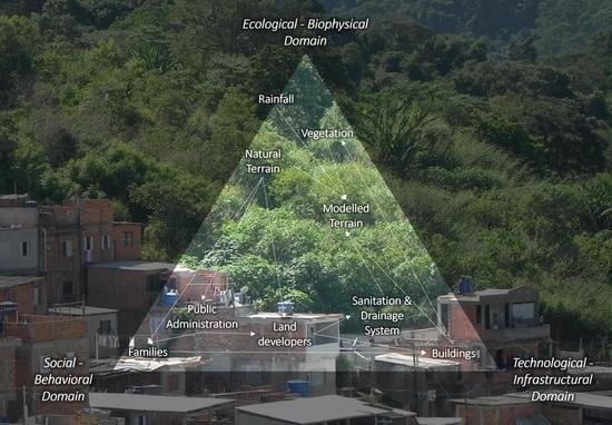
2. MRSP SETS’ Core Components
3. Materials and Methods
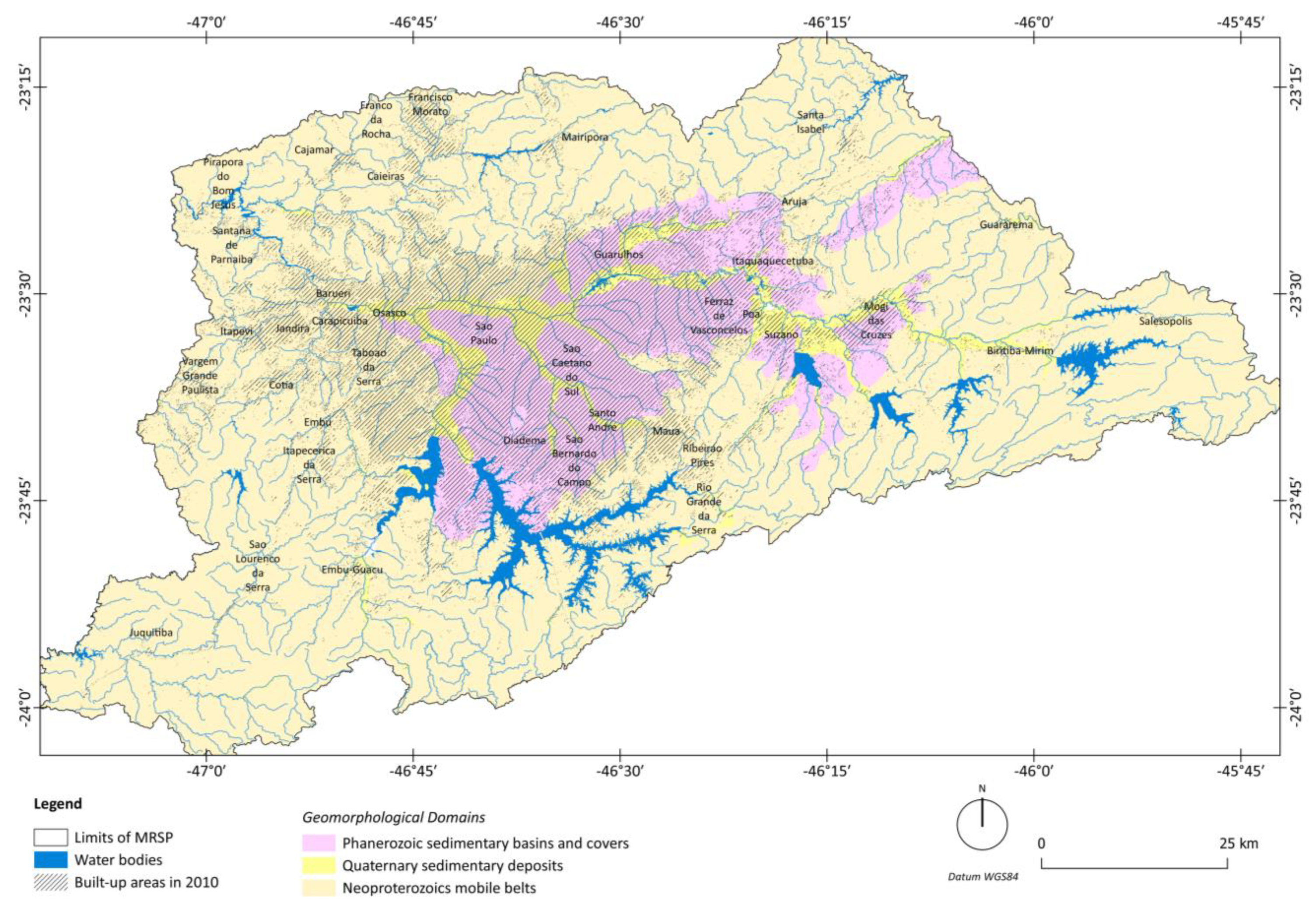
3.1. Study Area
3.2. Independent Variables
3.2.1. Landslide Inventory
3.2.2. Rainfall Data
3.2.3. Elevation-Related Variables
3.2.4. Physical Mass Movement Susceptibility
3.2.5. Land Cover Data
3.2.6. Demographic Census Data
3.3. Database Preparation
3.4. Model Development
3.5. Model Performance Assessment
4. Results
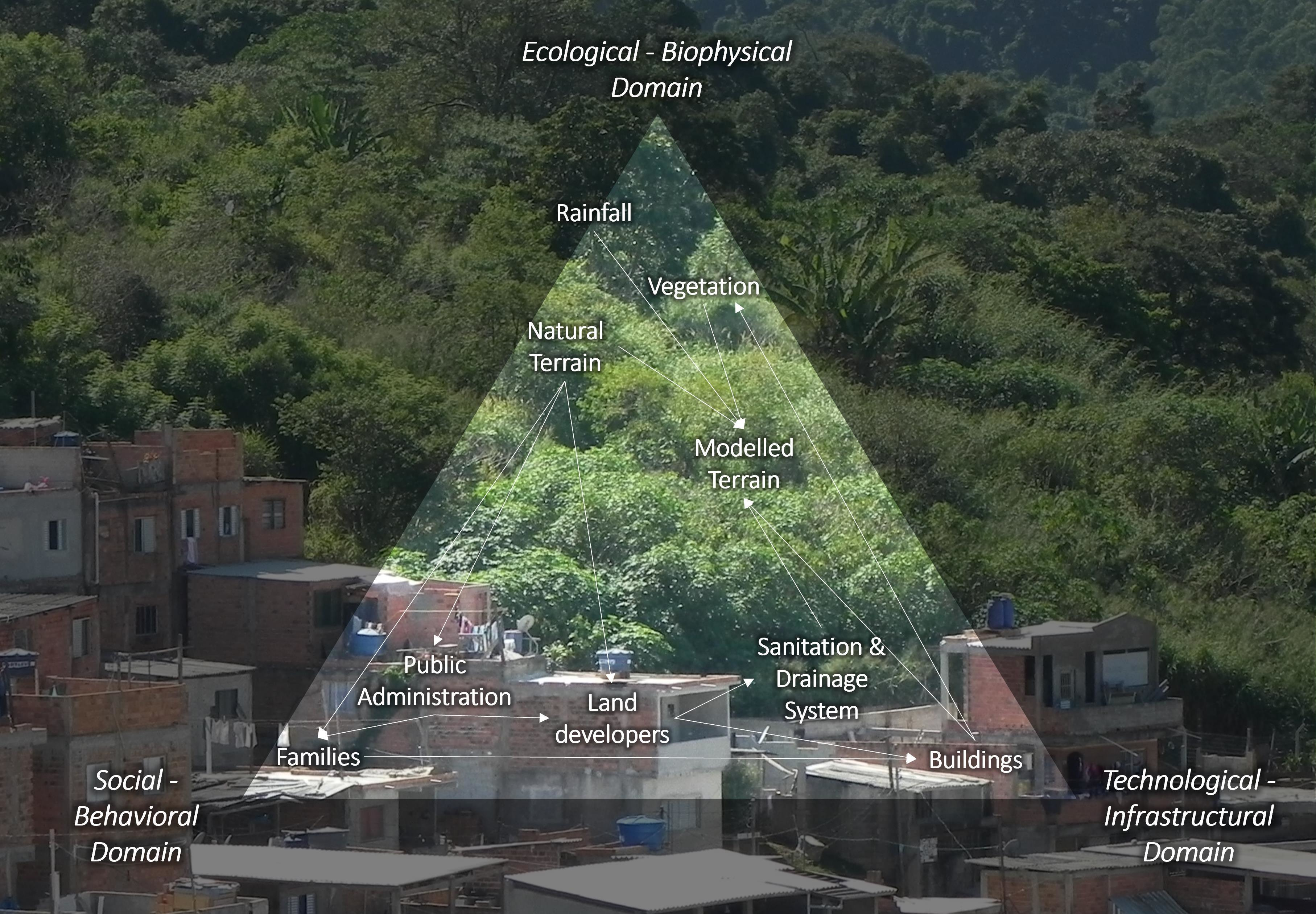
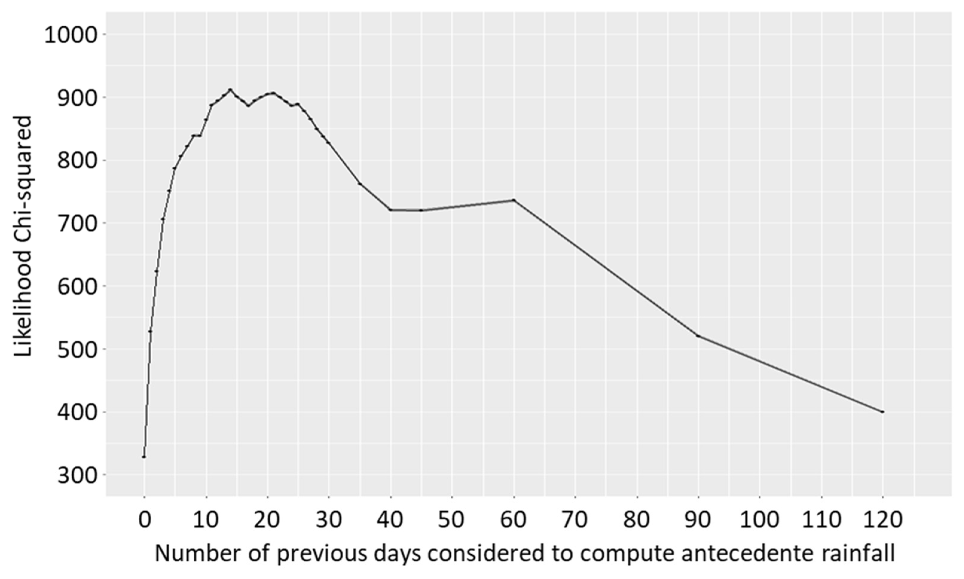
4.1. Antecedent Rainfall
4.2. Landslide occurrence Model
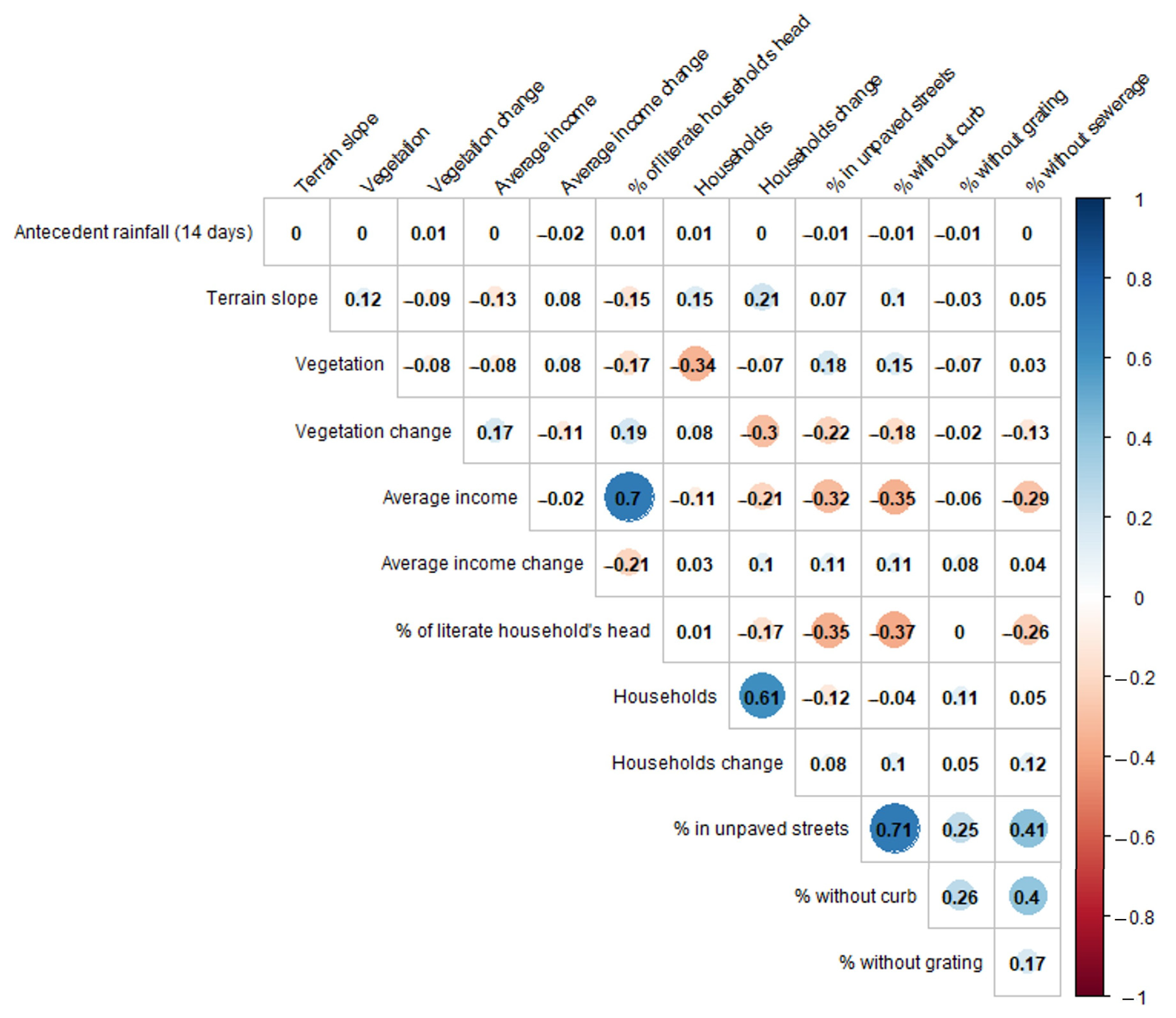
4.3. Variables’ Contribution
4.4. Landslide Occurrence Risk
5. Discussion
5.1. Importance of Ecological–Biophysical Variables in Landslide Occurrence
5.2. Importance of Social–Behavioral Variables in Landslide Occurrence
5.3. Importance of Technological–Infrastructural Variables in Landslide Occurrence
5.4. Landslide Occurrence from Social–Ecological–Technological System’s Perspective
5.5. Considerations for Urban Landslide Modeling
6. Conclusions
Author Contributions
Funding
Data Availability Statement
Acknowledgments
Conflicts of Interest
Appendix A. Model Development Results: Exploratory Analysis

| Independent Variable | Mean Value at Points of Landslide Occurrence | Mean Value at Points of Landslide Non-Occurrence | Student’s t-Test | p-Value |
|---|---|---|---|---|
| Rainfall in the event day | 18 mm | 6 mm | −31.45 | <0.001 |
| Antecedent rainfall—day and previous day | 37 mm | 11 mm | −42.89 | <0.001 |
| Antecedent rainfall—day and 7 previous days | 124 mm | 45 mm | −64.65 | <0.001 |
| Antecedent rainfall—day and 14 previous days | 216 mm | 83 mm | −71.67 | <0.001 |
| Antecedent rainfall—day and 21 previous days | 294 mm | 122 mm | −73.79 | <0.001 |
| Antecedent rainfall—day and 28 previous days | 367 mm | 162 mm | −70.41 | <0.001 |
| Antecedent rainfall—day and 60 previous days | 684 mm | 355 mm | −67.85 | <0.001 |
| Antecedent rainfall—day and 120 previous days | 1072 mm | 741 mm | −53.75 | <0.001 |
| Terrain slope | 14.45° | 7.09° | −32.43 | <0.001 |
| Percentage of vegetation in 2010 | 22.7% | 10.0% | −16.41 | <0.001 |
| Percentage of vegetation change (2010–1991) | −14.4% | −22.0% | −12.48 | <0.001 |
| Average income of the individual responsible for the household (household’s head) in 2010 | BRL 1828 (updated to 2018) | BRL 2647 (updated to 2018) | 29.52 | <0.001 |
| Average income change in the individual responsible for the household (household’s head) (2010–1991) | − BRL 1207 (updated to 2018) | − BRL 1137 (updated to 2018) | 2.15 | 0.032 |
| Percentage of literate individuals responsible for the household (household’s head) in 2010 | 95% | 95% | 2.31 | 0.021 |
| Households in 2010 | 20 households (222 households/ha) | 13 households (144 households/ha) | −17.46 | <0.001 |
| Household change (2010–1991) | 10 households | 6 households | −12.17 | <0.001 |
| Percentage of houses without sewerage in 2010 | 17.8% | 26.0% | 13.74 | <0.001 |
| Percentage of houses on unpaved streets in 2010 | 8.2% | 7.8% | −0.72 | 0.471 |
| Percentage of houses on streets without storm sewer (curb) in 2010 | 12.6% | 9.3% | −5.91 | <0.001 |
| Percentage of houses on streets without storm sewer (grating) in 2010 | 39.8% | 45.8% | 7.83 | <0.001 |
| Percentage of houses on streets with open sewage in 2010 | 4.6% | 6.0% | 5.08 | <0.001 |
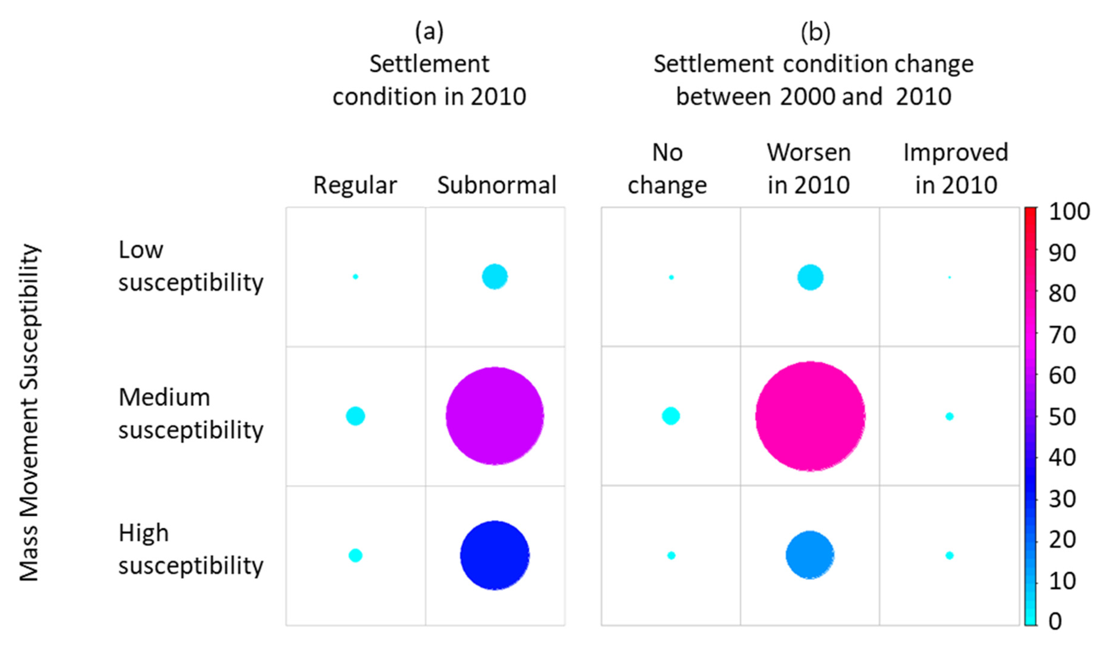
| Independent Variable and Categories | Number of Points of Landslide Occurrence 1 | Proportion at Points of Landslide Occurrence | Proportion at Points of Landslide Non-Occurrence | Pearson’s χ2 | d.f. | p-Value |
|---|---|---|---|---|---|---|
| Terrain aspect | 2038 | 170.94 | 4 | <0.001 | ||
| North | 464 | 22.77% | 18.55% | |||
| East | 306 | 15.01% | 21.91% | |||
| South | 479 | 23.50% | 16.59% | |||
| West | 491 | 24.09% | 21.64% | |||
| Flat | 298 | 14.62% | 21.31% | |||
| Mass movement susceptibility | 2037 | 1338.73 | 2 | <0.001 | ||
| Low | 1606 | 78.84% | 95.44% | |||
| Medium | 305 | 14.97% | 3.54% | |||
| High | 126 | 6.19% | 1.02% | |||
| Settlement condition in 2010 | 2038 | 1858.21 | 1 | <0.001 | ||
| Regular | 1592 | 78.12% | 96.26% | |||
| Subnormal | 446 | 21.88% | 3.74% | |||
| Settlement condition change (2010–2000) | 2038 | 396.87 | 2 | <0.001 | ||
| No change | 1839 | 90.24% | 97.18% | |||
| Worsened in 2010 | 180 | 8.83% | 2.29% | |||
| Improved in 2010 | 19 | 0.93% | 0.53% |


Appendix B. Model Development Results: Uni- and Multi-Variable Logistic Regression Assessment
| Univariable Models | Intercept | Coefficient | Coefficient Confidence Interval (95%) | p-Value | Likelihood Ratio χ2 |
|---|---|---|---|---|---|
| Antecedent rainfall (day and 14 previous days) | −2.4034 | 0.0160 | [0.0160, 0.0161] | <0.001 | 911.7 |
| Terrain slope | −0.9148 | 0.0885 | [0.0882, 0.0888] | <0.001 | 296.3 |
| Aspect | 0.1027 | 38.8 | |||
| North (in relation to flat areas) | −0.0104 | [−0.0178, −0.0029] | 0.578 | ||
| East (in relation to flat areas) | 0.4934 | [0.4858, 0.5010] | 0.008 | ||
| South (in relation to flat areas) | 0.6820 | [0.6742, 0.6897] | <0.001 | ||
| West (in relation to flat areas) | 0.3958 | [0.3884, 0.4033] | 0.031 | ||
| Mass movement susceptibility | −0.1870 | 130.5 | |||
| Medium (in relation to low) | 1.6395 | [1.6281, 1.6509] | <0.001 | ||
| High (in relation to low) | 1.9794 | [1.9579, 2.0008] | <0.001 | ||
| Percentage of vegetation in 2010 | −0.2445 | 1.6062 | [1.5976, 1.6148] | <0.001 | 94.0 |
| Percentage of vegetation change | 0.1536 | 0.8527 | [0.8449, 0.8605] | <0.001 | 32.9 |
| Average income of the household’s head in 2010 | 0.5021 | −0.0002 | [−0.0002, −0.0002] | <0.001 | 73.8 |
| Average income change for the household’s head | −0.023631 | −0.000021 | −0.000019] | 0.390 | 1.7 |
| Settlement condition in 2010 | −0.2097 | 162.4 | |||
| Subnormal (in relation to regular) | 1.9845 | [1.9737, 1.9954] | <0.001 | ||
| Settlement condition change | −0.0668 | 41.8 | |||
| Change (in relation to no change) | 1.4055 | [1.3918, 1.4192] | <0.001 | ||
| Households in 2010 | −0.5184 | 0.0319 | [0.0316, 0.0321] | <0.001 | 102.1 |
| Household change | −0.2174 | 0.0289 | [0.0286, 0.0292] | <0.001 | 54.7 |
| Percentage of households on streets without storm sewer (curb) in 2010 | −0.0615 | 0.5771 | [0.5666, 0.5876] | 0.025 | 9.3 |
| Percentage of households on streets without storm sewer (grating) in 2010 | 0.2189 | −0.5114 | [−0.5182, −0.5045] | 0.003 | 16.2 |
| Percentage of households on streets with open sewage in 2010 | 0.0384 | −0.7231 | [−0.7393, −0.7068] | 0.085 | 5.7 |
| Percentage of households without sewerage in 2010 | 0.1922 | −0.8958 | [−0.9032, −0.8884] | <0.001 | 38.8 |
| Variables of the Complete Model | Coefficient | Coefficient Confidence Interval (95%) | p-Value |
|---|---|---|---|
| Intercept | −3.4228 | [−3.4369, −3.4087] | <0.001 |
| Antecedent rainfall (day and 14 previous days) | 0.0164 | [0.0164, 0.0165] | <0.001 |
| Terrain slope | 0.0608 | [0.0604, 0.0613] | <0.001 |
| Mass movement susceptibility | |||
| Medium in relation to low | 0.2734 | [0.2573, 0.2894] | 0.399 |
| High in relation to low | −0.0008 | [−0.0358, 0.0343] | 0.517 |
| Percentage of vegetation in 2010 | 1.5938 | [1.5736, 1.6140] | 0,002 |
| Percentage of vegetation change | 0.3379 | [0.3242, 0.3516] | 0.293 |
| Average household head’s income in 2010 | −0.000123 | [−0.000125, −0.000121] | 0.012 |
| Settlement condition in 2010 | 1.9657 | [1.9424, 1.9889] | <0.001 |
| Settlement condition change | −0.9398 | [−0.9682, −0.9114] | 0.143 |
| Households in 2010 | 0.0384 | [0.0379, 0.0390] | 0.002 |
| Household change | −0.0051 | [−0.0057, −0.0045] | 0.477 |
| Percentage of households on streets without storm sewer (curb) in 2010 | 1.4845 | [1.4646, 1.5044] | 0.003 |
| Percentage of households on streets without storm sewer (grating) in 2010 | −0.1482 | [−0.1598, −0.1365] | 0.468 |
| Percentage of households on streets with open sewage in 2010 | −0.9120 | [−0.9394, −0.8846] | 0.182 |
| Percentage of households without sewerage in 2010 | −1.6121 | [−1.6264, −1.5978] | <0.001 |
| Observations (n) Points of landslide occurrence Points of landslide non-occurrence Bootstraps | 2000 1000 1000 1000 | Model likelihood test Likelihood ratio χ2 d.f. p-value | 1301.8 15 <0.001 |
References
- Alexander, D. Urban landslides. Prog. Phys. Geogr. Earth Environ. 1989, 13, 157–189. [Google Scholar] [CrossRef]
- Burton, I.; Kates, R.W.; White, G.F. The Environment as Hazard, 2nd ed.; The Guilford Press: New York, NY, USA; London, UK, 1993; ISBN 0-89862-159-3. [Google Scholar]
- Horlick, J.T. Urban disasters and megacities in a Risk society. GeoJournal 1995, 37, 329–334. [Google Scholar] [CrossRef]
- United Nations Office for Disaster Risk Reduction (UNDRR). Global Assessment Report on Disaster Risk Reduction; Geneva, Switzerland, 2019. Available online: https://www.undrr.org/media/73965 (accessed on 16 July 2019).
- Alexander, D. On the causes of landslides: Human activities, perception, and natural processes. Environ. Geol. Water Sci. 1992, 20, 165–179. [Google Scholar] [CrossRef]
- Ren, D. The devastating Zhouqu storm-triggered debris flow of August 2010: Likely causes and possible trends in a future warming climate. J. Geophys. Res. Atmos. 2014, 119, 3643–3662. [Google Scholar] [CrossRef]
- EM-DAT. The OFDA/CRED International Disaster Database; Centre for Research on the Epidemiology of Disasters, Université Catholique de Louvain: Ottignies-Louvain-la-Neuve, Belgium, 2019. [Google Scholar]
- Cui, Y.; Cheng, D.; Choi, C.E.; Jin, W.; Lei, Y.; Kargel, J.S. The cost of rapid and haphazard urbanization: Lessons learned from the Freetown landslide disaster. Landslides 2019, 16, 1167–1176. [Google Scholar] [CrossRef] [Green Version]
- Froude, M.J.; Petley, D.N. Global fatal landslide occurrence from 2004 to 2016. Nat. Hazards Earth Syst. Sci. 2018, 18, 2161–2181. [Google Scholar] [CrossRef] [Green Version]
- Petley, D.N. On the impact of urban landslides. In Engineering Geology for Tomorrow’s Cities; Culshaw, M.G., Reeves, H.J., Jefferson, I., Spink, T.W., Eds.; Geological Society: London, UK, 2009; Volume 22, pp. 83–99. [Google Scholar] [CrossRef]
- United Nations—Department of Economic and Social Affairs-Population Division. The World’s Cities in 2018—Data Booklet (No. St/Esa/Ser.A/417); United Nations: New York, NY, USA, 2018. [Google Scholar]
- Ab’saber, A. O sítio urbano de São Paulo. In A Cidade de São Paulo—Estudos de Geografia Urbana; de Azevedo, A., Ed.; Cia. Editora Nacional: São Paulo, Brazil, 1958; Volume I, pp. 169–248. Available online: http://www.brasiliana.com.br/obras/a-cidade-de-spaulo-estudos-de-geografia-urbana-v01/preambulo/4/texto (accessed on 12 September 2017).
- Instituto Geológico (IG). Cadastro Georreferenciado de Eventos Geodinâmicos: 50 Municípios da Região Metropolitana de São Paulo, Baixada Santista e Litoral Norte; Instituto Geológico: São Paulo, Brazil, 2017. Available online: https://www.infraestruturameioambiente.sp.gov.br/wp-content/uploads/sites/233/2017/12/Cad_Desastres_Shapefile_50mun.zip (accessed on 16 June 2019).
- United Nations Office for Disaster Risk Reduction (UNDRR). Global Assessment Report on Disaster Risk Reduction; United Nations Office for Disaster Risk Reduction: Geneva, Switzerland, 2009; Available online: https://www.undrr.org/publication/global-assessment-report-disaster-risk-reduction-2009 (accessed on 16 July 2019).
- Ceped. Atlas Brasileiro de Desastres Naturais: 1991 a 2012, 2nd ed.; CEPED UFSC: Florianópolis, Brazil, 2013; ISBN 9788564695085. [Google Scholar]
- Srivastava, A.; Babu, G.L.S.; Haldar, S. Influence of Spatial Variability of Permeability Property on Steady State Seepage Flow and Slope Stability Analysis. Eng. Geol. 2009, 110, 93–101. [Google Scholar] [CrossRef]
- Stanley, T.; Kirschbaum, D.B. A Heuristic Approach to Global Landslide Susceptibility Mapping. Nat. Hazards 2017, 87, 145–164. [Google Scholar] [CrossRef] [Green Version]
- Budimir, M.E.A.; Atkinson, P.M.; Lewis, H.G. A systematic review of landslide probability mapping using logistic regression. Landslides 2015, 12, 419–436. [Google Scholar] [CrossRef] [Green Version]
- Miao, F.; Zao, F.; Wu, Y.; Li, L.; Török, A. Landslide Susceptibility Mapping in Three Gorges Reservoir Area Based on GIS and Boosting Decision Tree Model. Stoch. Environ. Res. Risk Assess. 2023, 37, 2283–2303. [Google Scholar] [CrossRef]
- Zhang, R.; Chen, Y.; Zhang, X.; Ma, Q.; Ren, L. Mapping Homogeneous Regions for Flash Floods Using Machine Learning: A Case Study in Jiangxi Province, China. Int. J. Appl. Earth Obs. Geoinf. 2022, 108, 102717. [Google Scholar] [CrossRef]
- Yao, J.; Zhang, X.; Luo, W.; Liu, C.; Ren, L. Applications of Stacking/Blending Ensemble Learning Approaches for Evaluating Flash Flood Susceptibility. Int. J. Appl. Earth Obs. Geoinf. 2022, 112, 102932. [Google Scholar] [CrossRef]
- Aksha, S.K.; Resler, L.M.; Juran, L.; Carstensen, L.W. A geospatial analysis of multi-hazard risk in Dharan, Nepal. Geomat. Nat. Hazards Risk 2020, 11, 88–111. [Google Scholar] [CrossRef] [Green Version]
- Zeng, J.; Zhu, Z.Y.; Zhang, J.L.; Ouyang, T.P.; Qiu, S.F.; Zou, Y.; Zeng, T. Social Vulnerability Assessment of Natural Hazards on County-Scale Using High Spatial Resolution Satellite Imagery: A Case Study in the Luogang District of Guangzhou, South China. Environ. Earth Sci. 2012, 65, 173–182. [Google Scholar] [CrossRef]
- Chang, H.; Pallathadka, A.; Sauer, J.; Grimm, N.B.; Zimmerman, R.; Cheng, C.; Iwaniec, D.M.; Kim, Y.; Lloyd, R.; McPhearson, T.; et al. Assessment of Urban Flood Vulnerability Using the Social-Ecological-Technological Systems Framework in Six Us Cities. Sustain. Cities Soc. 2021, 68, 102786. [Google Scholar] [CrossRef]
- Arrogante-Funes, P.; Bruzón, A.G.; Arrogante-Funes, F.; Ramos-Bernal, R.N.; Vázquez-Jiménez, R. Integration of Vulnerability and Hazard Factors for Landslide Risk Assessment. Int. J. Environ. Res. Public Health 2021, 18, 11987. [Google Scholar] [CrossRef]
- Ahmed, B. The Root Causes of Landslide Vulnerability in Bangladesh. Landslides 2021, 18, 1707–1720. [Google Scholar] [CrossRef]
- Kumar, D.; Bhattacharjya, R.K. Study of Integrated Social Vulnerability Index Sovi of Hilly Region of Uttarakhand, India. Environ. Clim. Technol. 2019, 24, 105–122. [Google Scholar] [CrossRef] [Green Version]
- Pickett, S.T.A.; Cadenasso, M.L.; Grove, J.M.; Boone, C.G.; Groffman, P.M.; Irwin, E.; Kaushal, S.S.; Marshall, V.; McGrath, B.P.; Nilon, C.H.; et al. Urban ecological systems: Scientific foundations and a decade of progress. J. Environ. Manag. 2011, 92, 331–362. [Google Scholar] [CrossRef] [PubMed]
- Mcphearson, T.; Haase, D.; Kabisch, N. Advancing understanding of the complex nature of urban systems. Ecol. Indic. 2016, 70, 566–573. [Google Scholar] [CrossRef]
- Depietri, Y.; Mcphearson, T. Integrating the Grey, Green, and Blue in Cities: Nature-Based Solutions for Climate Change Adaptation and Risk Reduction. In Nature-Based Solutions to Climate Change Adaptation in Urban Areas; Braubach, M., Egorov, A., Mudu, P., Wolf, T., Thompson, C.W., Martuzzi, M., Eds.; Springer: Berlin/Heidelberg, Germany, 2017. [Google Scholar] [CrossRef]
- Grabowski, Z.J.; Matsler, A.M.; Thiel, C.; Mcphillips, L.; Hum, R.; Bradshaw, A.; Redman, C. Infrastructures as Socio-Eco-Technical Systems: Five Considerations for Interdisciplinary Dialogue. J. Infrastruct. Syst. 2017, 23, 02517002. [Google Scholar] [CrossRef]
- Markolf, S.A.; Chester, M.V.; Eisenberg, D.A.; Iwaniec, D.M.; Davidson, C.I.; Zimmerman, R.; Chang, H. Interdependent Infrastructure as Linked Social, Ecological, and Technological Systems (SETSs) to Address Lock-in and Enhance Resilience. Earth’s Future 2018, 6, 1638–1659. [Google Scholar] [CrossRef] [Green Version]
- Mcphearson, T.; Pickett, S.T.A.; Grimm, N.B.; Niemelä, J.; Alberti, M.; Elmqvist, T.; Qureshi, S. Advancing Urban Ecology toward a Science of Cities. BioScience 2016, 66, 198–212. [Google Scholar] [CrossRef] [Green Version]
- Bai, X.; Surveyer, A.; Elmqvist, T.; Gatzweiler, F.W.; Güneralp, B.; Parnell, S.; Webb, R. Defining and advancing a systems approach for sustainable cities. Curr. Opin. Environ. Sustain. 2016, 23, 69–78. [Google Scholar] [CrossRef]
- Guidicini, G.; Iwasa, O.Y. Tentative correlation between rainfall and landslides in a humid tropical environment. Bull. Int. Assoc. Eng. Geol. 1977, 16, 13–20. [Google Scholar] [CrossRef]
- Schuster, R.L.; Highland, L.M. The Third Hans Cloos Lecture. Urban landslides: Socioeconomic impacts and overview of Mitigative strategies. Bull. Eng. Geol. Environ. 2007, 66, 1–27. [Google Scholar] [CrossRef]
- Ávila, A.; Justino, F.; Wilson, A.; Bromwich, D.; Amorim, M. Recent precipitation trends, flash floods and landslides in southern Brazil. Environ. Res. Lett. 2016, 11, 114029. [Google Scholar] [CrossRef]
- Segoni, S.; Piciullo, L.; Gariano, S.L. A review of the recent literature on rainfall thresholds for landslide occurrence. Landslides 2018, 15, 1483–1501. [Google Scholar] [CrossRef]
- Dai, F.C.; Lee, C.F. A spatiotemporal probabilistic modelling of storm-induced shallow landsliding using aerial photographs and logistic regression. Earth Surf. Process. Landf. 2003, 28, 527–545. [Google Scholar] [CrossRef]
- Santoro, J.; Mendes, R.M.; Pressinotti, M.M.N.; Manoel, G.R. Correlação Entre Chuvas e Deslizamentos Ocorridos Durante a Operação do Plano Preventivo De Defesa Civil. In Proceedings of the 7th Simpósio Brasileiro de Cartografia Geotécnica e Geoambiental, Maringá, Brazil, 8–11 August 2010. [Google Scholar]
- Tatizana, C.; Ogura, A.T.; Cerri, L.E.S.; Rocha, M.C.M. Modelamento numérico da análise de correlação entre chuvas e escorregamentos aplicado às encostas da Serra do Mar no município de Cubatão. In Proceedings of the 5th Congresso Brasileiro de Geologia de Engenharia; ABGE: São Paulo, Brazil, 1987; Volume 2, pp. 237–248. [Google Scholar]
- Pasuto, A.; Silvano, S. Rainfall as a trigger of shallow mass movements. A case study in the Dolomites, Italy. Environ. Geol. 1998, 35, 184–189. [Google Scholar] [CrossRef]
- Mendes, R.M.; de Andrade, M.R.M.; Tomasella, J.; de Moraes, M.A.E.; Scofield, G.B. Understanding shallow landslides in Campos do Jordão municipality-Brazil: Disentangling the anthropic effects from natural causes in the disaster of 2000. Nat. Hazards Earth Syst. Sci. 2018, 18, 15–30. [Google Scholar] [CrossRef] [Green Version]
- Guzzetti, F.; Reichenbach, P.; Bartoccini, P.; Galli, M.; Ardizzone, F.; Cardinali, M. Rainfall induced landslides in December 2004 in south-western Umbria, central Italy: Types, extent, damage and risk assessment. Nat. Hazards Earth Syst. Sci. 2006, 6, 237–260. [Google Scholar]
- Kirschbaum, D.; Stanley, T. Satellite-Based Assessment of Rainfall-Triggered Landslide Hazard for Situational Awareness. Earth’s Future 2018, 6, 505–523. [Google Scholar] [CrossRef] [PubMed]
- Guzzetti, F.; Peruccacci, S.; Rossi, M.; Stark, C.P. Rainfall thresholds for the initiation of landslides in central and southern Europe. Meteorol. Atmos. Phys. 2007, 98, 239–267. [Google Scholar] [CrossRef]
- Instituto Geológico (IG). Relatório Da Operação Dos Planos Preventivos De Defesa Civil—PPDC: Operação Verão 2016–2017; Instituto Geológico: São Paulo, Brazil, 2017. Available online: https://www.infraestruturameioambiente.sp.gov.br/wp-content/uploads/sites/233/2017/11/RELAT_PPDC_2016-2017_FINAL.pdf (accessed on 15 June 2019).
- Ahrendt, A.; Zuquette, L.V. Triggering factors of landslides in Campos do Jordão city, Brazil. Bull. Eng. Geol. Environ. 2003, 62, 231–244. [Google Scholar] [CrossRef]
- Smyth, C.G.; Royle, S.A. Urban landslide hazards: Incidence and causative factors in Niteroi, Rio de Janeiro state, Brazil. Appl. Geogr. 2000, 20, 95–118. [Google Scholar] [CrossRef]
- Chau, K.T.; Chan, J.E. Regional bias of landslide data in generating susceptibility maps using logistic regression: Case of Hong Kong Island. Landslides 2005, 2, 280–290. [Google Scholar] [CrossRef]
- Süzen, M.L.; Kaya, B.Ş. Evaluation of environmental parameters in logistic regression models for landslide susceptibility mapping. Int. J. Digit. Earth 2012, 5, 338–355. [Google Scholar] [CrossRef]
- Varnes, D.J. Slope Movement Types and Processes (special report No. 176). In Landslides: Analysis and Control; Schuster, R.L., Krizek, R.J., Eds.; Transportation Research Board, National Research Council: Washington, DC, USA, 1978. [Google Scholar]
- Bitar, O.Y. (Ed.) Cartas de Susceptibilidade a Movimentos Gravitacionais de Massa e Inundações—1:25.000: Nota Técnica Explicativa; Instituto de Pesquisas Tecnológicas do Estado de São Paulo (IPT): São Paulo, Brazil; Serviço Geológico do Brasil (CPRM): Brasília, Brazil, 2014. [Google Scholar]
- Kanungo, D.; Arora, M.; Sarkar, S.; Gupta, R. Landslide Susceptibility Zonation (LSZ) Mapping–A Review. J. South Asia Disaster Stud. 2009, 2, 81–105. [Google Scholar]
- Ross, J.L.S. Inundações e deslizamentos em São Paulo: Riscos da relação inadequada sociedade-natureza. Territorium 2016, 8, 15–23. [Google Scholar] [CrossRef] [Green Version]
- Alexander, D. Vulnerability to Landslides. In Landslide Hazard and Risk; Glade, T., Anderson, M., Crozier, M.J., Eds.; John Wiley & Sons, Ltd.: Hoboken, NJ, USA, 2005; pp. 175–198. [Google Scholar] [CrossRef]
- Imaizumi, F.; Sidle, R.C.; Kamei, R. Effects of forest harvesting on the occurrence of landslides and debris flows in steep terrain of central Japan. Earth Surf. Process. Landf. 2008, 33, 827–840. [Google Scholar] [CrossRef]
- Peloggia, A.U.G. Delineação e Aprofundamento Temático da Geologia do Tecnógeno do Município de São Paulo. Ph.D. Thesis, Universidade de São Paulo, Instituto de Geociências, São Paulo, Brazil, 1997. [Google Scholar]
- Mirandola, F.A.; de Macedo, E.S. Proposta de classificação do tecnógeno para uso no mapeamento de áreas de risco de deslizamento. Quat. Environ. Geosci. 2014, 5, 66–81. [Google Scholar] [CrossRef]
- Blaikie, P.; Cannon, T.; Davis, I.; Wisner, B. At Risk: Natural Hazards, People’s Vulnerability and Disasters; Routledge: London, UK, 1994. [Google Scholar] [CrossRef]
- Peloggia, A.U.G.; Silva, F.A.N.; Takyia, H.; Barros, L.H.S.; Fujimoto, N.A.; Figueiredo, R.B. Riscos geológicos e geotécnicos em áreas de precária ocupação urbana no município de São Paulo; Sociedade Brasileira de Geologia: São Paulo, Brazil, 1992. [Google Scholar] [CrossRef]
- Farah, F. Habitação e Encostas; Instituto de Pesquisas Tecnológicas: São Paulo, Brazil, 2003; Publicação IPT; p. 2795. [Google Scholar]
- Marcondes, M.J.D.A. Cidade e Natureza. Proteção dos Mananciais e Exclusão Social, 1st ed.; Studio Nobel, Edusp, Fapesp: São Paulo, Brazil, 1999. [Google Scholar]
- Instituto Brasileiro de Geografia e Estatística (IBGE). Manual Técnico de Geomorfologia (Manuais Técnicos em Geociências No. 5); Instituto Brasileiro de Geografia e Estatística: Rio de Janeiro, Brazil, 2009; ISBN 9788524042225. [Google Scholar]
- Empresa Paulista de Planejamento Metropolitano S.A. (EMPLASA). Folhas Planialtimétricas da Região Metropolitana de São Paulo—1980/1981 (com atualizações); EMPLASA: São Paulo, Brazil, 1980; Scale: 1:10.000. [Google Scholar]
- Sepe, P.M.; Takiya, H. Atlas Ambiental da Cidade de São Paulo; Secretaria Municipal do Verde e do Meio Ambiente (SVMA): São Paulo, Brazil, 2000. [Google Scholar]
- Nobre, C.A.; Young, A.F.; Saldiva, P.H.N.; Orsini, J.A.M.; Nobre, A.D.; Ogura, A.; Rodrigues, G.D.O. Vulnerabilidades das Megacidades Brasileiras às Mudanças Climáticas: Região Metropolitana de São Paulo; Instituto Nacional de Pesquisas Espaciais: São José dos Campos, Brazil; Universidade Estadual de Campinas: Campinas, Brazil, 2011. [Google Scholar]
- Xavier, T.M.B.S.; Xavier, A.F.S.; Silva Dias, M.A.F.D. Evolução da precipitação diária num ambiente urbano: O caso da cidade de São Paulo. Rev. Bras. Meteorol. 1994, 9, 44–53. [Google Scholar]
- Funk, C.; Peterson, P.; Landsfeld, M.; Pedreros, D.; Verdin, J.; Shukla, S.; Husak, G.; Rowland, J.; Harrison, L.; Hoell, A.; et al. The climate hazards infrared precipitation with stations - A new environmental record for monitoring extremes. Sci. Data 2015, 2, 150066. [Google Scholar] [CrossRef] [Green Version]
- Horn, B.K.P. Hill-Shading and the Reflectance Map. Proc. IEEE 1981, 69, 14–47. [Google Scholar] [CrossRef] [Green Version]
- Instituto Brasileiro de Geografia e Estatística (IBGE). Censo Demográfico 1991 (No. 21); Instituto Brasileiro de Geografia e Estatística: Rio de Janeiro, Brazil, 1991. Available online: https://www.ibge.gov.br/estatisticas/sociais/populacao/25089-censo-1991-6.html?edicao=25090 (accessed on 18 June 2019).
- Instituto Brasileiro de Geografia e Estatística (IBGE). Metodologia do Censo Demográfico 2010 (Série Relatórios Metodológicos No. 41; Série Relatórios Metodológicos (Vol. 41); Instituto Brasileiro de Geografia e Estatística: Rio de Janeiro, Brazil, 2013. [Google Scholar]
- Joint Research Centre (JRC)—European Commission. Documentation for the GHS Population Grid, Derived from Gpw4, Multitemporal (1975, 1990, 2000, 2015) (GHS-Pop); European Commission: Ispra, Italy, 2017. [Google Scholar]
- Langford, M.; Unwin, D.J. Generating and mapping population density surfaces within a geographical information system. Cartogr. J. 1994, 31, 21–26. [Google Scholar] [CrossRef] [PubMed]
- Holt, J.B.; Lo, C.P.; Hodler, T.W. Dasymetric Estimation of Population Density and Areal Interpolation of Census Data. Cartogr. Geogr. Inf. Sci. 2004, 31, 103–121. [Google Scholar] [CrossRef]
- Hirye, M.C.M.; McPhearson, T.; Filardo Jr., A.S.; Alves, D.S. Demographic, economic and physical data integration: Measuring hillside’s urban occupation in Metropolitan Region of São Paulo (Brazil). In Proceedings of the Proceedings American Geophysical Union Fall Meeting 2018, Washington, DC, USA, 10–14 December 2018. Abstract Number IN33B-0859. [Google Scholar]
- Fell, R.; Whitt, G.; Miner, T.; Flentje, P. Guidelines for landslide susceptibility, hazard and risk zoning for land use planning. Eng. Geol. 2008, 102, 83–84. [Google Scholar] [CrossRef] [Green Version]
- Glade, T.; Crozier, M.J. Landslide Hazard and Risk—Concluding Comment and Perspectives. In Landslide Hazard and Risk; Glade, T., Anderson, M., Crozier, M.J., Eds.; John Wiley & Sons, Ltd.: Chichester, England, 2005; pp. 765–774. [Google Scholar] [CrossRef]
- Van Westen, C.J.; Castellanos, E.; Kuriakose, S.L. Spatial data for landslide susceptibility, hazard, and vulnerability assessment: An overview. Eng. Geol. 2008, 102, 112–131. [Google Scholar] [CrossRef]
- Brenning, A. Spatial prediction models for landslide hazards: Review, comparison and evaluation. Nat. Hazards Earth Syst. Sci. 2005, 5, 853–862. [Google Scholar] [CrossRef]
- Steyerberg, E.W.; Harrell, F.E.; Borsboom, G.J.J.; Eijkemans, M.J.; Vergouwe, Y.; Habbema, J.D.F. Internal validation of predictive models: Efficiency of some procedures for logistic regression analysis. J. Clin. Epidemiol. 2001, 54, 774–781. [Google Scholar] [CrossRef] [PubMed]
- Efron, B.; Robert, J.T. An Introduction to the Bootstrap; Chapman & Hall/Crc: Boca Raton, FL, USA, 1994. [Google Scholar]
- Harrell, F.E. Regression Modeling Strategies; Springer International Publishing: Cham, Switzerland, 2015. [Google Scholar] [CrossRef]
- Hosmer, D.W.; Lemeshow, S. Applied Logistic Regression, 2nd ed.; John Wiley & Sons, Inc.: Hoboken, NJ, USA, 2000. [Google Scholar]
- Smith, T.J.; Mckenna, C.M. A comparison of logistic regression pseudo R2 indices. Mult. Linear Regres. Viewp. 2013, 39, 17–26. [Google Scholar]
- Schwarz, G. Estimating the Dimension of a Model. Ann. Stat. 1978, 6, 461–464. [Google Scholar] [CrossRef]
- Kirschbaum, D.; Kapnick, S.B.; Stanley, T.; Pascale, S. Changes in Extreme Precipitation and Landslides Over High Mountain Asia. Geophys. Res. Lett. 2020, 47. [Google Scholar] [CrossRef]
- El Kharim, Y.; Bounab, A.; Ilias, O.; Hilali, F.; Ahniche, M. Landslides in the urban and suburban perimeter of Chefchaouen (Rif, Northern Morocco): Inventory and case study. Nat. Hazards 2021, 107, 355–373. [Google Scholar] [CrossRef]
- Ehrlich, M.; Luiz, B.J.; Mendes, C.G.; Lacerda, W.A. Triggering factors and critical thresholds for landslides in Rio de Janeiro-Rj, Brazil. Nat. Hazards 2021, 107, 937–952. [Google Scholar] [CrossRef]
- Bezerra, L.; Neto, O.D.F.; Santos, O., Jr.; Mickovski, S. Landslide Risk Mapping in an Urban Area of the City of Natal, Brazil. Sustainability 2020, 12, 9601. [Google Scholar] [CrossRef]
- Cascini, L.; Bonnard, C.; Corominas, J.; Jibson, R.W.; Montero-Olarte, J. Landslide risk evaluation and hazard zoning for rapid and long-travel landslides in urban development areas. In Landslide Risk Management; Taylor and Francis: London, UK, 2005; pp. 199–235. [Google Scholar] [CrossRef]


| Domain | Independent Variable |
|---|---|
| Ecological–Biophysical Domain | Daily rainfall |
| Antecedent rainfall | |
| Terrain slope | |
| Terrain aspect | |
| Mass movement susceptibility | |
| Percentage of vegetation in 2010 | |
| Percentage of vegetation change (2010–1991) | |
| Social–Behavioral Domain | Average income of the individual responsible for the household in 2010 |
| Average change in income of the individual responsible for the household (2010–1991) | |
| Percentage of literate individuals responsible for the household (household’s head) in 2010 | |
| Settlement condition in 2010 | |
| Settlement condition change (2010–1991) | |
| Technological–Infrastructural Domain | Households in 2010 |
| Household changes (2010–1991) | |
| Percentage of households without sewerage in 2010 | |
| Percentage of households on unpaved streets in 2010 | |
| Percentage of households on streets without storm sewer (curb) in 2010 | |
| Percentage of households on streets without storm sewer (grating) in 2010 | |
| Percentage of households on streets with open sewage in 2010 |
| Variables of Final Model | Coefficient | Coefficient Confidence Interval (95%) | p-Value |
|---|---|---|---|
| Intercept | −3.5869 | [−3.5997, −3.5740] | <0.001 |
| Antecedent rainfall (day and 14 previous days) | 0.0163 | [0.0162, 0.0163] | <0.001 |
| Terrain slope | 0.0621 | [0.0617, 0.0625] | <0.001 |
| Percentage of vegetation in 2010 | 1.7894 | [1.7699, 1.8089] | <0.001 |
| Average household head’s income in 2010 | −0.0001 | [−0.0001, −0.0001] | 0.019 |
| Settlement condition in 2010 | 1.5335 | [1.5180, 1.5489] | <0.001 |
| Households in 2010 | 0.0370 | [0.0365, 0.0374] | <0.001 |
| Percentage of households on streets without storm sewer (curb) in 2010 | 1.1494 | [1.1329, 1.1659] | 0.007 |
| Percentage of households without sewerage in 2010 | −1.7180 | [−1.7317, −1.7044] | <0.001 |
| Final model | |||
| Observations (n) Points of landslide occurrence Points of landslide non-occurrence Bootstraps | 2000 1000 1000 1000 | Model likelihood test Likelihood ratio χ2 d.f. p-value | 1280.3 8 <0.001 |
| Final Model and Models with Subset of Selected Variables | Rank | Number of Times as Rank #1 | BIC Value | BIC Value Confidence Interval (95%) |
|---|---|---|---|---|
| Final model | 1 | 549 | 1561 | [1559, 1564] |
| Final model, except average household head’s income in 2010 | 2 | 274 | 1557 | [1554, 1559] |
| Final model, except percentage of households on streets without storm sewer (curb) in 2010 | 3 | 155 | 1559 | [1556, 1562] |
| Variable | Likelihood Ratio χ2 | Adequacy |
|---|---|---|
| Antecedent rainfall (day and 14 previous days) | 900.6 | 0.70 |
| Terrain slope | 262.2 | 0.20 |
| Percentage of vegetation in 2010 | 20.7 | 0.02 |
| Average household head’s income in 2010 | 73.7 | 0.06 |
| Settlement condition in 2010 | 191.3 | 0.15 |
| Households in 2010 | 174.9 | 0.14 |
| Percentage of households on streets without storm sewer (curb) in 2010 | 16.9 | 0.01 |
| Percentage of households without sewerage in 2010 | 24.5 | 0.02 |
| Combined | 1280.3 | 1.00 |
| Variable | Increment | Odds Ratio | Odds Ratio Confidence Interval (95%) |
|---|---|---|---|
| Antecedent rainfall (day and 14 previous days) | 10 mm | 1.177 | [1.176, 1.177] |
| Terrain slope | 1° | 1.064 | [1.064, 1.065] |
| Percentage of vegetation in 2010 | 10% | 1.196 | [1.194, 1.199] |
| Average household head’s income in 2010 | BRL 10,000 | 0.989 | [0.9887, 0.9891] |
| Settlement condition in 2010 | Subnormal in relation to regular | 4.634 | [4.705, 4.863] |
| Households in 2010 | 1 household | 1.038 | [1.037, 1.038] |
| Percentage of households on streets without storm sewer (curb) in 2010 | 10% | 1.122 | [1.120, 1.124] |
| Percentage of households without sewerage in 2010 | 10% | 0.842 | [0.841, 0.843] |
Disclaimer/Publisher’s Note: The statements, opinions and data contained in all publications are solely those of the individual author(s) and contributor(s) and not of MDPI and/or the editor(s). MDPI and/or the editor(s) disclaim responsibility for any injury to people or property resulting from any ideas, methods, instructions or products referred to in the content. |
© 2023 by the authors. Licensee MDPI, Basel, Switzerland. This article is an open access article distributed under the terms and conditions of the Creative Commons Attribution (CC BY) license (https://creativecommons.org/licenses/by/4.0/).
Share and Cite
Hirye, M.C.M.; Alves, D.S.; Filardo Jr., A.S.; McPhearson, T.; Wagner, F. Assessing Landslide Drivers in Social–Ecological–Technological Systems: The Case of Metropolitan Region of São Paulo, Brazil. Remote Sens. 2023, 15, 3048. https://doi.org/10.3390/rs15123048
Hirye MCM, Alves DS, Filardo Jr. AS, McPhearson T, Wagner F. Assessing Landslide Drivers in Social–Ecological–Technological Systems: The Case of Metropolitan Region of São Paulo, Brazil. Remote Sensing. 2023; 15(12):3048. https://doi.org/10.3390/rs15123048
Chicago/Turabian StyleHirye, Mayumi C. M., Diógenes Salas Alves, Angelo Salvador Filardo Jr., Timon McPhearson, and Fabien Wagner. 2023. "Assessing Landslide Drivers in Social–Ecological–Technological Systems: The Case of Metropolitan Region of São Paulo, Brazil" Remote Sensing 15, no. 12: 3048. https://doi.org/10.3390/rs15123048