
Assimilating All-Sky Infrared Radiance Observations to Improve Ensemble Analyses and Short-Term Predictions of Thunderstorms

1
Institute of Atmospheric Physics, Chinese Academy of Sciences, Beijing 100029, China
2
Cooperative Institute for Severe and High-Impact Weather Research and Operations, University of Oklahoma, Norman, OK 73072, USA
3
University of Chinese Academy of Sciences, Beijing 100029, China
4
NOAA/OAR/National Severe Storms Laboratory, Norman, OK 73072, USA
*
Author to whom correspondence should be addressed.
Remote Sens. 2023, 15(12), 2998; https://doi.org/10.3390/rs15122998
Submission received: 28 April 2023
/
Revised: 26 May 2023
/
Accepted: 28 May 2023
/
Published: 8 June 2023
(This article belongs to the Special Issue Remote Sensing Data Application, Data Reanalysis and Advances for Mesoscale Numerical Weather Models)
Abstract
:The experimental rapid-cycling Ensemble Kalman Filter (EnKF) in the convection-allowing ensemble-based Warn-on-Forecast System (WoFS) at the National Severe Storms Laboratory (NSSL) is used to assimilate all-sky infrared radiance observations from the GOES-16 7.3 μm water vapor channel in combination with radar wind and reflectivity observations to improve the analysis and subsequent forecast of severe thunderstorms (which occurred in Oklahoma on 2 May 2018). The method for radiance data assimilation is based primarily on the version used in WoFS. In addition, the methods for adaptive observation error inflation and background error inflation and the method of time-expanded sampling are also implemented in two groups of experiments to test their effectiveness and examine the impacts of radar observations and all-sky radiance observations on ensemble analyses and predictions of severe thunderstorms. Radar reflectivity observations and brightness temperature observations from the GOES-16 6.9 μm mid-level troposphere water vapor channel and 11.2 μm longwave window channel are used to evaluate the assimilation statistics and verify the forecasts in each experiment. The primary findings from the two groups of experiments are summarized: (i) Assimilating radar observations improves the overall (heavy) precipitation forecast up to 5 (4) h, according to the improved composite reflectivity forecast skill scores. (ii) Assimilating all-sky water vapor infrared radiance observations from GOES-16 in addition to radar observations improves the brightness temperature assimilation statistics and subsequent cloud cover forecast up to 6 h, but the improvements are not significantly affected by the adaptive observation and background error inflations. (iii) Time-expanded sampling can not only reduce the computational cost substantially but also slightly improve the forecast.
1. Introduction
Assimilation of microwave radiance data from polar orbiting satellites has led to substantial forecast improvements for global numerical weather prediction (NWP) systems [1,2,3]. However, all-sky infrared assimilation is not yet operational, although many operational centers are looking to activate the water vapor sounding channels. Data from geostationary satellites, such as the Advanced Baseline Imager (ABI) on board the GOES-R series, have high temporal-spatial resolutions, making them much more suitable for the data requirements of high-resolution mesoscale NWP systems compared with polar-orbiting satellite data. The ABI samples 16 channels that have important sensitivities to atmospheric temperature and moisture properties and are available at a 2 km horizontal resolution every 10–15 min with a data latency of only a few minutes [4]. The low data latency is crucial for the convection-allowing Warn-on-Forecast System (WoFS), which assimilates data at 15 min intervals or less over a regional domain in a real-time fashion to generate short-term (0–6 h) forecasts of high-impact weather events [5,6]. Motivated by this low data latency, several studies assimilated GOES satellite data in conjunction with other high-resolution datasets, such as radar reflectivity and radial velocity, to complement the advantages of each and increase skill in high-impact weather prediction [6,7,8,9,10].
In addition to conventional observations, reflectivity and radial-velocity observations from ground-based Doppler radars form the basic input observations for the WoFS. However, geostationary satellite data sample non-precipitating clouds and environmental conditions with high temporal-spatial resolutions not readily sensed by radars. Assimilation of even just the clear-sky portion of these data into the WoFS can often improve the analyses and subsequent forecasts [7]. Geostationary satellite data are also useful in providing information on convection in the absence of radars, but a truly successful WoFS does require reasonable radar data coverage to reliably generate consistently skillful forecasts. Geostationary satellite data can be assimilated in different forms, such as radiances, Brightness Temperatures (BT) or retrievals. Each form has its advantages and disadvantages, but both convey important environmental and cloud properties to the data assimilation system. Jones et al. [6] assimilated Cloud Water Path (CWP) retrievals into the WoFS and demonstrated improvement in the forecasting of cloud properties, convective initiation, and the near-storm environment compared with experiments that only assimilated radar data. Jones et al. [7] further experimented with assimilating GOES-13 6.95 μm clear-sky water vapor channel radiances in combination with radar and CWP and showed that assimilating radiances did improve the model analysis, leading to improvements in the forecasting of rotating severe storms. However, the correction of inherent model biases caused a degradation in one case.
Recently, by making an initial attempt at assimilating all-sky radiances into the WoFS, Jones et al. [8] studied the relative impacts of assimilating GOES-16 all-sky water vapor channel radiances at 6.2, 6.9, and 7.3 μm wavelengths compared with other radar and satellite observations. Similar results were obtained through assimilating all-sky water vapor channel radiances [9,10]. These studies showed that assimilating all-sky radiances can have very positive impacts in certain conditions, as it improved the Convective Initiation (CI) forecast of severe storms in several instances. However, the retrieval method with clear-sky radiances performs best in some cases, especially after CI. Following their initial attempt, this paper aims to further study the impacts of assimilating GOES-16 all-sky water vapor channel infrared radiance observations into the WoFS on improving the analysis and subsequent prediction of thunderstorms for the severe storm event that occurred in the central southern US on 2 May 2018. The method for water vapor radiance data assimilation used in this paper is based primarily on the studies of Jones et al. [7,8]. In addition, we will apply the methods of Adaptive Observation Error Inflation (AOEI) [11] and Adaptive Background Error Inflation (ABEI) [12] to the rapid-cycling Ensemble Kalman Filter (EnKF) in the WoFS and test their impacts on the analyses and subsequent predictions. We will also apply the Time-Expanded Sampling (TES) method [13,14] to the rapid-cycling EnKF in the WoFS and test its effectiveness in reducing the computational cost for assimilating all-sky water vapor radiance observations.
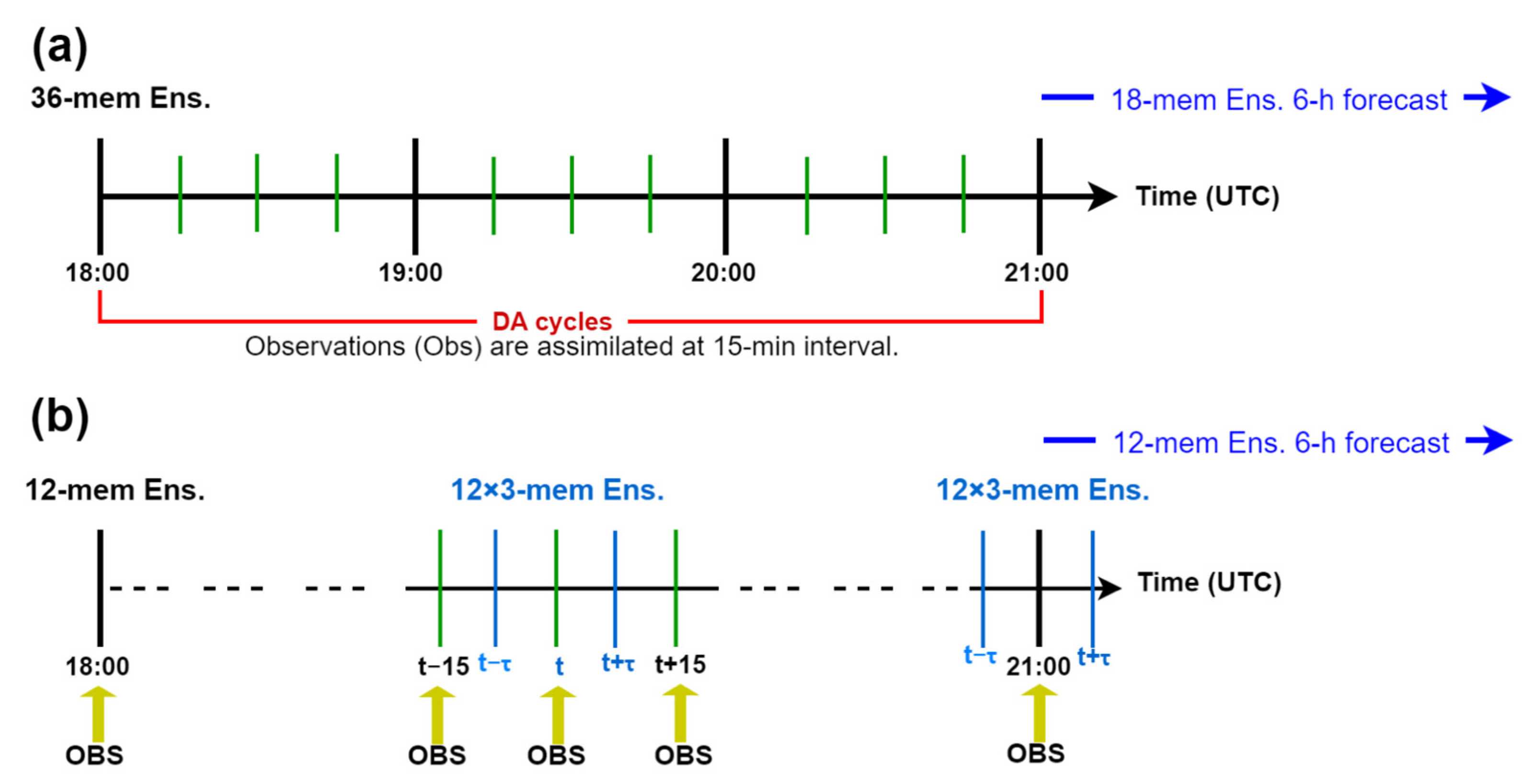
As explained in Xu et al. [13,14], the idea behind the TES technique was inspired by the fact that model-predicted weather systems often develop and/or propagate either faster or slower than those observed in the real atmosphere. In this case, the predicted field at a time level before or after the analysis time may better represent the true state than the one at the analysis time, so the difference between the predicted field sampled before or after the analysis time and the one at the analysis time may represent, to a certain extent, the model’s forecast errors in intensity and/or location of the predicted weather system. By sampling perturbed state vectors from each ensemble forecast at additional time levels shifted, say by ±τ, from the analysis time, TES can not only sample timing and/or phase errors but also triple the analysis ensemble size for covariance construction without increasing the ensemble size in forecast updates. The method was also called the Valid-Time-Shifting method (VTS) in some recent studies [15,16], but this paper still uses the name TES as originally proposed by Xu et al. [13,14]. Although TES was shown to be useful and effective for EnKF assimilations of real radar observations over mesoscale and synoptic-scale domains [16,17,18], radars, and geostationary satellite GOES-16 clear-sky observations from two water vapor channels at 6.2 and 7.3 μm wavelengths [19], the method has not been tested with an EnKF to assimilate GOES-16 all-sky observations from water vapor channels in addition to radar observations for short-term (0–6 h) forecasts of severe storms. Such a test will be performed in this study with the rapid-cycling EnKF in the WoFS.
The next section describes the WoFS configuration, its rapid-cycling EnKF, and the observations assimilated in this paper. Section 3 overviews the severe weather event and designs the assimilation experiments with brief descriptions of verification methods. Section 4 presents the experiment results, and provides qualitative and quantitative comparisons between different assimilation experiments. Conclusions follow in Section 5.
2. WoFS and Rapid-Cycling EnKF
The WoFS is an ensemble data assimilation and forecasting system designed to generate short-term (0–6 h) forecasts of severe thunderstorms and flash flooding. The WoFS uses an EnKF approach to assimilate conventional, radar, and satellite data at a 3 km horizontal resolution and 51 vertical levels in a regional domain [5,6]. The WoFS uses a modified version of the Advanced Weather Research and Forecasting Model (WRF-ARW), version 3 [20], coupled with a modified version of the community’s v3.7 Gridpoint Statistical Interpolation (GSI) system [21]. Modifications include new radar forward operators and a capability to assimilate high-resolution GOES Advanced Baseline Imager (ABI) data. The v3.7 GSI contains the Community Radiative Transfer Model (CRTM version 2.3) as a forward observation operator that translates model state variables into simulated satellite radiances for comparison with observations [22]. The GSI-EnKF system includes forward observation operators for radar reflectivity and radial velocity, CWP [6], and conventional observations [8].
All observations are assimilated using an EnKF to generate flow-dependent covariances and update the model state in each assimilation cycle [23]. In this paper, the EnKF is cycled every 15 min beginning at 1800 UTC up to 3 h at 2100 UTC, followed by ensemble forecast runs up to 6 h until 0300 UTC the next day (Figure 1a). This EnKF can assimilate all available conventional, radar, and satellite observations during the 3 h period (from 1800 to 2100 UTC) into a 36-member ensemble. Initial and boundary conditions are provided by an experimental 36-member High-Resolution Rapid Refresh Ensemble (HRRRE [24]) using 1 h forecasts from the 1600 UTC analysis and forecasts generated from the first nine members of the 1200 UTC cycle, respectively. For the 2018 thunderstorm case considered in this paper, the WoFS regional domain has 250 × 250 grid points with 3 km grid resolution, and this domain is nested within the HRRRE. All ensemble members use the two-moment NSSL variable density cloud microphysics scheme [25]. During each cycle, temperature, humidity, wind, pressure, diabatic heating, and hydrometeor variables are updated.
Ensemble spread is maintained by applying different sets of model boundary layer physics and radiation schemes to each member. Horizontal and vertical localizations are applied using the Gaspari and Cohn method [26] and are varied as a function of observation types. Conventional observations have the longest (60 km) localization length, while high-density radar data have the smallest (18 km) localization length. Radar reflectivity observations are derived from the Multi-Radar Multi-Sensor (MRMS) product created from the Weather Surveillance Doppler Radar 88D (WSR-88D) network [27,28]. Negative reflectivity values are set to zero during the MRMS preprocessing phase, and the data are further thinned to a 5 km resolution. Reflectivity values between 0 and 15 dBZ are not assimilated to provide a buffer between precipitation and non-precipitation (defined by 0 dBZ) regions. Radial velocity observations are created using the raw level II WSR-88D data, which are dealiased and also objectively analyzed to a 5-km resolution. Only radial velocity observations within 150 km of a particular radar that lies near or within the domain are used.
For conventional observations (temperature, dewpoint, winds, and pressure from the Oklahoma Mesonet), radar reflectivity and radial-velocity observations, observation error standard deviations, and localization radii and depths are specified in Table 1. Among the three water vapor channels of GOES-16, all-sky infrared BT observations from the water vapor channel at 7.3 μm wavelength (BT73) are assimilated in this paper, and this channel (band 10) is sensitive to low-level troposphere water vapor content in clear-sky regions with peak weighting functions of 625 hPa assuming a standard atmosphere. Since the slantwise nature of the observation between the surface and the satellite results in a displacement error in the geolocation of a cloud in satellite imagery compared with its ground truth location, a parallax correction is applied for cloudy radiances using the method described in [6]. In particular, as described in [6], since the geolocation of the raw satellite data measures the physical condition of the cloud at its top and not its base, the horizontal locations at the surface and aloft are not the same when the satellite is not directly overhead. To correct for parallax, the retrieved cloud height is used to remap cloudy pixels to their zenith location above the surface. The observation error standard deviations and localization radii and depths specified for BT73 under clear and cloudy conditions are listed in the last two rows of Table 1.
3. Event Overviews and Experiment Design
3.1. Event Overviews
The severe weather event that occurred on 2 May 2018 was selected to study the impacts of assimilating satellite data in addition to radar and conventional observations (from the Oklahoma Mesonet), the impacts of using adaptive observation and background error inflations, and the usefulness of TES. This case generated multiple instances of high-impact weather, including tornadoes in addition to large hail and damaging straight-line winds.
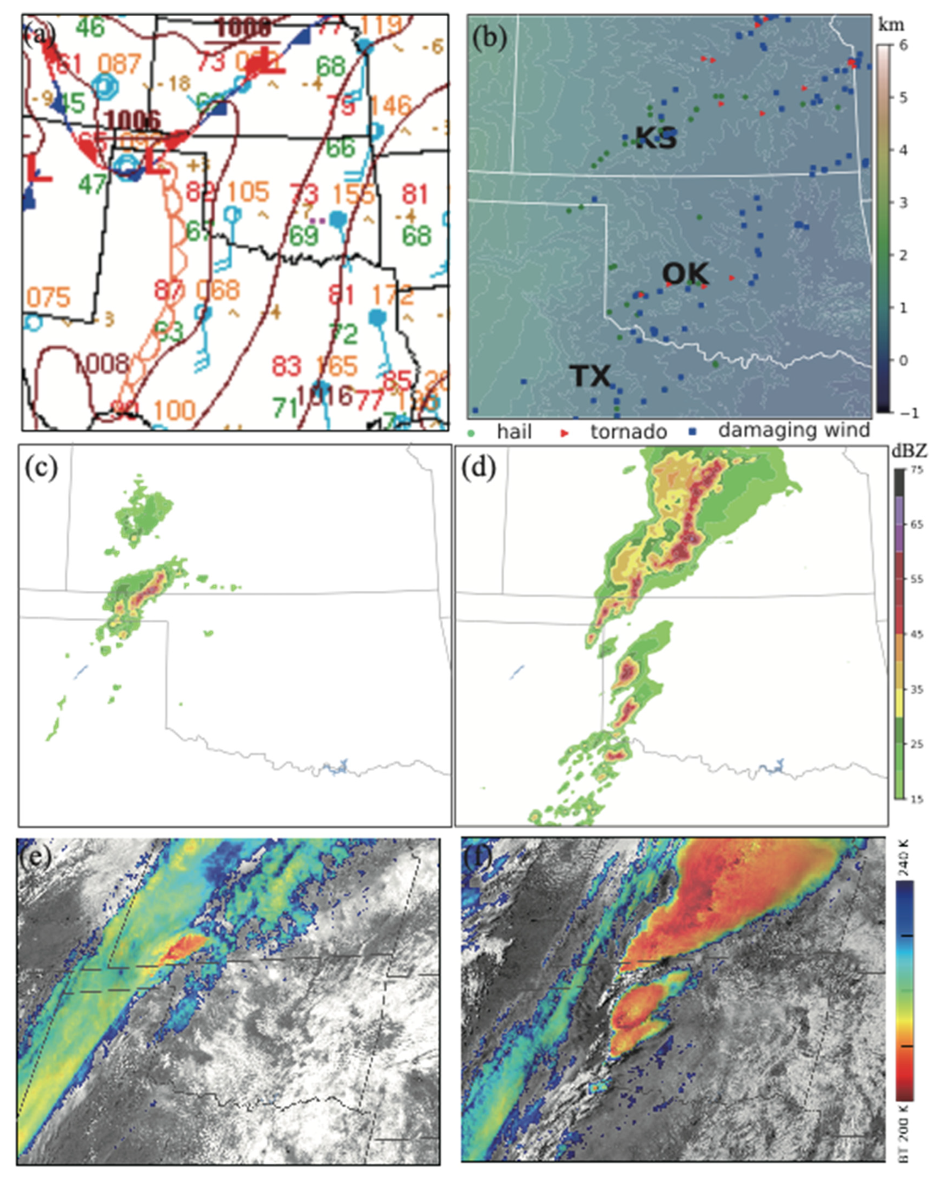
On 2 May 2018, two clusters of storm cells, initialized along and ahead of a quasi-stationary front and a dryline, respectively (Figure 2a,c,e), developed and moved eastward through the central Great Plains of the US (Figure 2d). [Note that in Figure 2a the line composed of interlaced blue and red segments (with a bule triangle attached on each blue segment and a red semicircles attached on each red segment) marks the quasi-stationary front, the light orange line (attached with hollow semicircles) marks the dry line, the dark orange lines are the surface pressure contours (in mb labeled by dark orange numbers), and the wind barb is plotted in light blue with the sky/cloud cover symbol at the location of each surface station where the surface temperature and dew point are shown by the red and green numbers (in °F) on the top-left and bottom-left, respectively, and the surface pressure is shown by the yellow number (in mb above 1000 mb) on the top-right.] There were 11 tornadoes reported in Kansas from 2105 to 0215 UTC. In addition, four tornadoes were reported in Oklahoma from 2138 to 0144 UTC (Figure 2b). Hail up to tennis ball size was reported in Wichita, Kansas, at 2117 UTC and as large as a medium-sized hen egg in north Texas at 2152 UTC. These strong storms were accompanied by heavy precipitation, with more than 50 mm falling in central Oklahoma between 0000 and 0100 UTC. Satellite data also show a north–south-oriented band of upper-level cirrus clouds overrunning the region where the Kansas storm develops (Figure 2f).
3.2. Experiment Design
Two groups of experiments are designed. The first group consists of one control experiment and four impact-test experiments designed to test the impacts of assimilating radar and GOES-16 all-sky radiance in addition to conventional observations and also to test the additional impacts of AOEI and ABEI [11,12] in assimilating GOES-16 all-sky radiance. In this group, the control experiment, named E-CONV, assimilates only the conventional observations (from the Oklahoma Mesonet). The first impact-test experiment, named E-RADAR, assimilates operationally available radar observations in addition to conventional observations. The second impact-test experiment, named E-BT73, assimilates GOES-16 all-sky BT73 in addition to those used in the first impact-test experiment, and the experiment design is based primarily on the studies of Jones et al. [7,8]. The third impact-test experiment, named E-AOEI, is designed to test the additional impact of AOEI. The fourth impact-test experiment, named E-AOBEI, is designed to test the impact of ABEI in addition to AOEI. In these last two impact-test experiments, the adaptive error inflation methods are used together with the method of Relaxing Posterior Spread to Prior Spread (RTPS) with the relaxation coefficient set to 0.9, as in E-RADAR and E-BT73 (see Table 2). In each of the four impact-test experiments, an additive noise technique is used to perturb model state variables where observed reflectivity is greater than a given threshold [29].
The second group consists of one control experiment and three TES experiments designed to examine the effectiveness of TES in reducing the computational cost of assimilating all-sky water vapor radiance observations with the WoFS. In this group, the control experiment is simply taken from the first impact-test experiment in the first group (that is, E-BT73). As listed in Table 3, E-BT73 uses the baseline configuration as described for the WoFS in Section 2, which has 36 ensemble members in EnKF data assimilation updating runs and 18 members in forecast runs. The three TES experiments, named TES225, TES300, and TE450, focus on the cost-saving feature of TES by reducing the ensemble size from 36 to 12 (see Table 2) in WoFS EnKF data assimilation updating runs with the shifting time interval set to τ = 225, 300, and 450 s, respectively, while reducing the ensemble size in forecast runs to 12.
3.3. Verification Methods
Reflectivity observations processed as MRMS products from the WSR-88D Doppler radar network will be used as ground truth to verify WoFS forecasted reflectivity up to 6 h in each experiment. Infrared BT observations from the GOES-16 mid-level troposphere water vapor channel (band 9) at 6.9 μm wavelength (BT69) and the infrared longwave window channel (band 14) at 11.2 μm wavelength (BT112) will be used as ground truths to verify WoFS forecasted BT69 and BT112, respectively, for up to 6 h in each experiment. The accuracies of the forecasted composite reflectivity field and two BT fields from each experiment will be measured by the Root Mean Square Errors (RMSEs) computed against their respective ground truths. Furthermore, the accuracy of the forecasted composite reflectivity field will also be measured by the equitable threat scores (ETS) [30] computed with different thresholds against corresponding MRMS products.
4. Experiment Results and Comparisons
4.1. Assimilation Statistics for the First Group of Experiments
The ensemble spread in the space of a given type of observation is defined and denoted by
where ∑m denotes the summation over integer m from 1 to M—the number of assimilated observations of the given type, ∑n denotes the summation over integer n from 1 to N—the ensemble size represented by the number of ensemble members, xn denotes the model state vector represented by the nth ensemble member, and Hm denotes the operator that maps xn to the observation type and location of the mth observation. With xn given by the prior (forecast) or posterior (analysis), the prior (posterior) ensemble spread is calculated for each type of remote sensing immediately before (after) the analysis time in each assimilation cycle. The calculated ensemble spread s forms a zig-zag function of time (from 1800 to 2100 UTC) as it reduces from a prior to a posterior value immediately after the analysis in each assimilation cycle before increasing to a prior value during the next assimilation cycle.
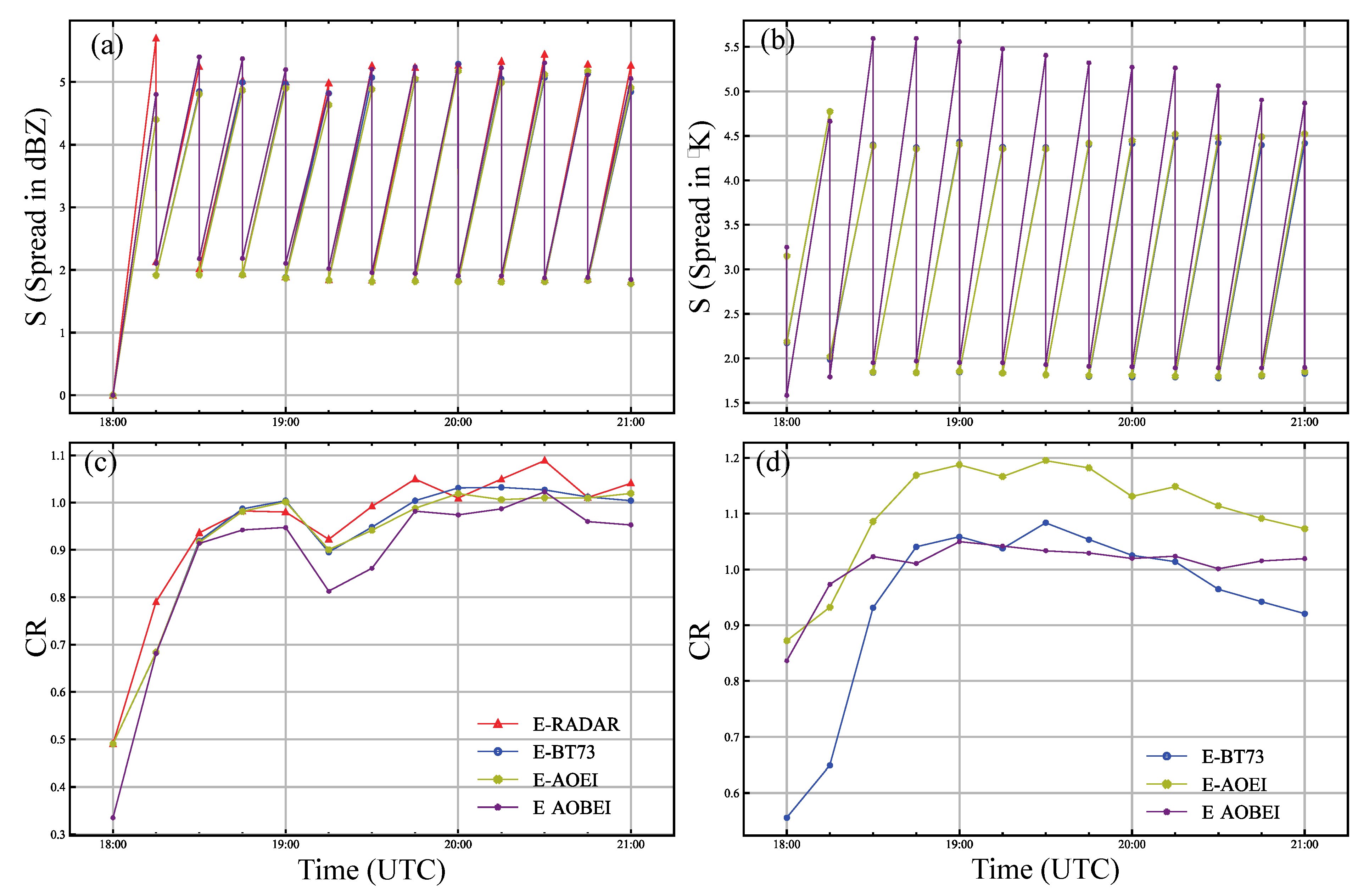
The reflectivity ensemble spreads calculated from the four impact-test experiments are plotted by four differently colored zig-zag curves in Figure 3a. As shown in Figure 3a, the reflectivity ensemble spreads from the four impact-test experiments have about the same zig-zag variations, especially after the third assimilation cycle, although the zig-zag variations of the spread from E-AOBEI are slightly larger than those from E-BT73 and E-AOEI during the first two assimilation cycles. Thus, the reflectivity ensemble spreads are not much affected by assimilating BT73, regardless of whether ABEI and/or AOEI are used.
Figure 3b shows that the BT73 ensemble spreads from E-BT73 and E-AOEI have nearly the same zig-zag variations, but the zig-zag variations of the spread from E-AOBEI are significantly larger than those from E-BT73 and E-AOEI after the second assimilation cycle and before the second-to-last assimilation cycle. Thus, the BT73 ensemble spreads are not much affected by the use of AOEI but are significantly affected by the use of ABEI because ABEI inflates the background error variances in temperature, water vapor, and rainwater that cause the BT73 ensemble spread to increase.
For a given type of observation, we denote by ym the mth observation and by Hm(x) the ensemble mean mapped into the mth observation, where x denotes the model state vector represented by the ensemble mean and Hm denotes the operator that maps x to the observation type and location of the mth observation. We then define and denote the root-mean-square innovation by
where ∑m is the same as in (1), dm ≡ ym − Hm(x) is the innovation with respect to the ensemble mean mapped into the mth observation, and d ≡ ∑mdm/M. Since ym and Hm(x) represent the same truth, dm ≡ ym − Hm(x) can be written into dm = om − em, where om and em denote the errors of ym and Hm(x), respectively, while d’m ≡ dm − d can be written into d’m = o’m − e’m, where o’m ≡ om − ∑mom/M and e’m ≡ em − ∑mem/M denote the random errors in ym and Hm(x), respectively. With x given by the prior (forecast) ensemble mean, ∑mo’me’m should be zero or nearly so due to the independence between o’m and e’m. In this case, we have
where σo2 is observation error variance and e’m2 ≈ ∑n[Hm(xn) − ∑nHm(xn)/N]2/(N − 1) is used to estimate the error variance of the prior (forecast) ensemble mapped to the observation type and location of the mth observation. Here, Equation (3) gives a diagnostic tool that can be employed for a consistency check. In particular, if the forecast error variance is well estimated by prior s2, the consistency relationship in (3) should be well satisfied, and the Consistency Ratio (CR) defined by
will be close to 1.
The CRs calculated for reflectivity from the four impact-test experiments are plotted by four differently colored curves in Figure 3c. As shown in Figure 3c, the reflectivity CRs from the four experiments are below 0.5 (especially the one from E-AOBEI) at the beginning of the first assimilation cycle but increase rapidly toward 1 during the first three cycles. The reflectivity CRs from E-BT73 and E-AOEI are very close to each other and very close to 1 during the last 6 cycles, while the reflectivity CR from E-RADAR (E-AOBEI) is slightly above (below) 1 most of the time during the last 6 cycles. These results imply that assimilating BT73 (without using ABEI) in addition to radar data can slightly improve the ensemble estimated background error variance for reflectivity, and the estimated error variance is not much affected by the use of AOEI but degraded slightly by the use of ABEI.
Figure 3d shows that the BT73 CR from E-BT73 is around 0.55 at the beginning of the first assimilation cycle but increases rapidly to 1.04 during the first three cycles and then varies slowly between 0.92 and 1.08. On the other hand, the BT73 CR from E-AOEI (E-AOBEI) is 0.88 (0.84) at the beginning of the first assimilation cycle, increases rapidly to 1.18 (1.01) during the first three cycles, and then varies slowly between 1.19 and 1.08 (1.00 and 1.05). Clearly, the use of AOEI degrades the BT73 CR, while the use of ABEI improves the BT73 CR, and this improvement can be explained by the ABEI-inflated background error variance for BT73 (see Figure 3b and related explanations). The above results imply that the ensemble estimated background error variance for BT73 is slightly degraded (improved) by the use of AOEI (ABEI).
4.2. Forecast Performances for the First Group of Experiments
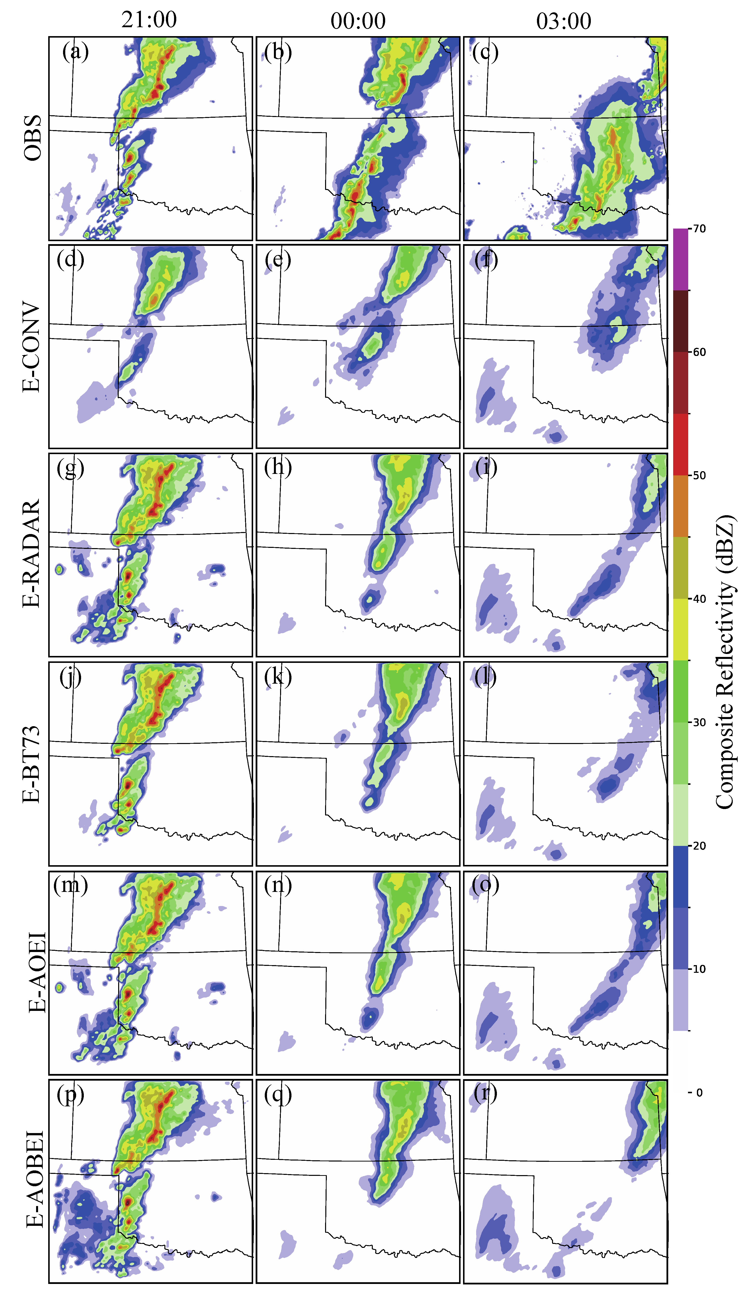
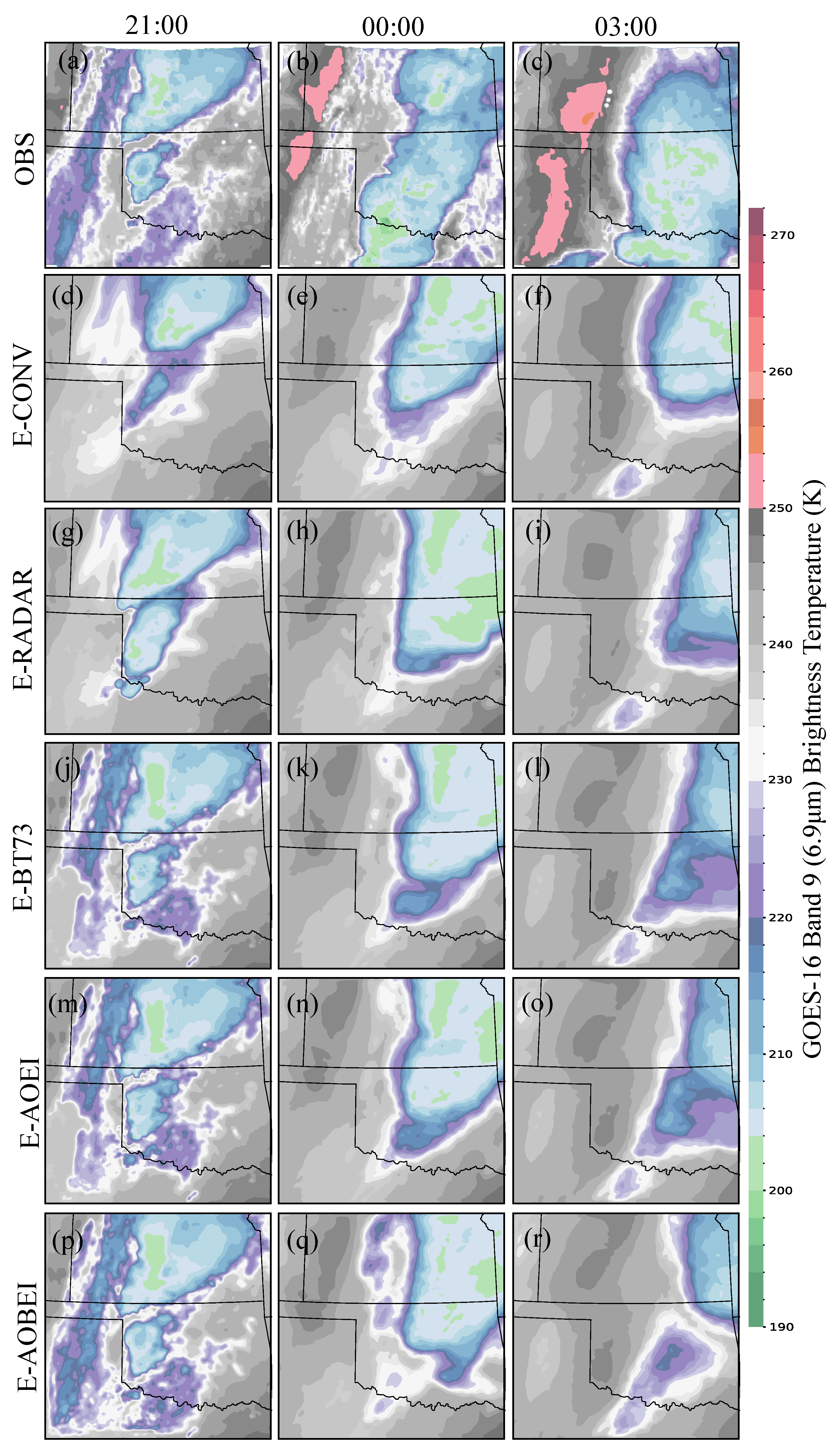
Composite reflectivity observations processed as MRMS products from the WSR-88D Doppler radar network are plotted as ground truths in the first row of Figure 4 to verify the forecasted composite reflectivity ensemble means at 0, 3, and 6 h forecast lead times valid at 2100 and 0000 UTC and 0300 UTC the next day, respectively, from each experiment in each subsequent row of Figure 4. From the first column of Figure 4, we can see that the 0 h forecasted (that is, the analyzed at the end of the last assimilation cycle) composite reflectivity ensemble mean from E-CONV is not very close to the one observed in Figure 4a, but the closeness to the observed one is improved significantly when reflectivity observations are assimilated in E-RADAR. Further assimilating BT73 in E-BT73 does not further improve the closeness, although it removes small areas of spurious weak composite reflectivity on the two sides of the precipitation band along the west border of Oklahoma. Further using AOEI also does not further improve the closeness, and using AOBI slightly worsens the closeness to the observed one.
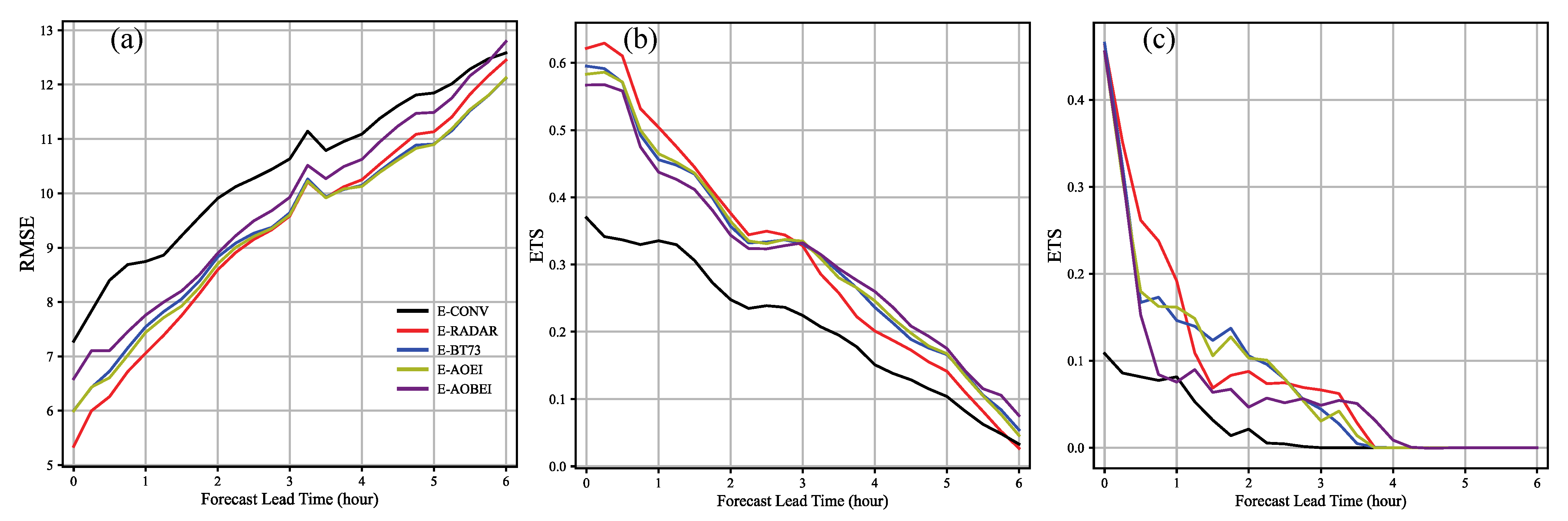
The second (third) column of Figure 4 shows that the forecasted composite reflectivity ensemble means from the five experiments all become less (much less) close to the values observed in Figure 4b (c) as the forecast lead time increases to 3 (6) h. At 3 h forecast lead time, the forecasted ensemble means from E-RADAR, E-BT73, and E-AOEI are quite close to each other and much closer (slightly closer) to the observed one than that from E-CONV (E-AOBEI). At 6 h forecast lead time, the forecasted ensemble means from E-BT73 and E-AOEI are still close to each other but become less close to the observed one than that from E-RADAR, although they are still much closer (closer) to the observed one than that from E-CONV (E-AOBEI). The above comparisons are confirmed quantitatively by the RMSE of the forecasted composite reflectivity ensemble mean plotted in Figure 5a as a function of the forecast lead time for each experiment in the first group.
Relative to the forecasted composite reflectivity ensemble mean from E-CONV, the Degree of Forecast Improvement (DFI) from E-RADAR or E-BT73 can be measured in percentage by DFI = (RMSEconv − RMSE)/RMSEconv, where RMSEconv denotes the RMSE from E-CONV and RMSE denotes the reduced RMSE from E-RADAR or E-BT73. According to the results in Figure 5a, the DFI is 10.3% for the 3 h forecast from either E-RADAR or E-BT73. When the forecast lead time increases to 5 h, the DFI is reduced to 5.9% (8.4%) for the forecast from E-RADAR (E-BT73).
The ETSs of forecasted composite reflectivity ensemble means calculated using 20 and 40 dBZ thresholds from the five experiments in the first group are plotted by five differently colored curves as functions of forecast lead time in Figure 5b,c, respectively. As shown in Figure 5b, at 0 h forecast lead time, the ETS calculated using the 20 dBZ threshold from E-CONV is much lower than those from the four impact-test experiments, while the ETS from E-RADAR (E-BT73) is the highest (second highest), and the ETS from E-AOEI is slightly lower (higher) than that from E-BT73 (E-AOBEI). As the forecast time increases to 3 h, the ETSs from the four impact-test experiments all decrease to 0.33, while the ETS from E-CONV decreases to 0.22. As the forecast time further increases to 6 h, the ETS from E-AOBEI decreases most slowly to 0.08, while the ETSs from E-BT73 and E-AOEI decrease to about 0.06 and the ETSs from E-RADAR and E-CONV decrease to about 0.04. The above results indicate indirectly that assimilating reflectivity observations improves the overall precipitation forecast up to 5 h, and further assimilating BT73 slightly degrades (improves) the forecast before (after) 3 h forecast lead time, while using AOEI, ABEI, or both does not much further affect the forecast.
Figure 5c shows that at 0 h forecast lead time, the ETSs calculated using the 40 dBZ threshold from the four impact-test experiments are all around 0.44, while the ETS from E-CONV is very low (≈0.1). As the forecast time increases to 1 h, the ETS from E-AOBEI decreases most rapidly to about the same level of 0.09 as the ETS from E-CONV, the ETSs from E-BT73 and E-AOEI decrease less rapidly to about 0.16, and the ETS from E-RADAR decreases to about 0.19. As the forecast time further increases to 3 h, the ETS from E-CONV diminishes, and the ETSs from E-RADAR, E-BT73, E-AOEI, and E-AOBEI decrease to about 0.075, 0.05, 0.04, and 0.05, respectively. As the forecast time increases to 4 h, the ETS from E-AOBEI decreases to 0.05, and the ETSs from the remaining three impact-test experiments all diminish. These results indicate indirectly that assimilating reflectivity observations improves heavy precipitation forecasts nearly up to 4 h, and further assimilating BT73 slightly degrades (improves) the forecast before 1 h forecast lead time and after 3 h forecast lead time (between 1 h and 3 h forecast lead times), while using AOEI does not much affect the forecast and using ABEI does not improve the forecast until the forecast lead time increases beyond 3 h (but the ETS score reduces to nearly 0.05).
BT69 observations are plotted as ground truths in the first row of Figure 6 to verify the forecasted BT69 ensemble means at 0 h, 3 h, and 6 h forecast lead times valid at 2100 UTC, 0000, and 0300 UTC the next day, respectively, from each experiment in each subsequent row of Figure 6. As shown in the first column of Figure 6, the 0 h forecasted BT69 ensemble mean from E-CONV is not close to the observed one in Figure 6a, and the closeness to the observed one is slightly improved by assimilating reflectivity observations in E-RADAR and significantly improved by further assimilating BT73 in E-BT73, but not affected (further improved) by using AOEI (AOBI).
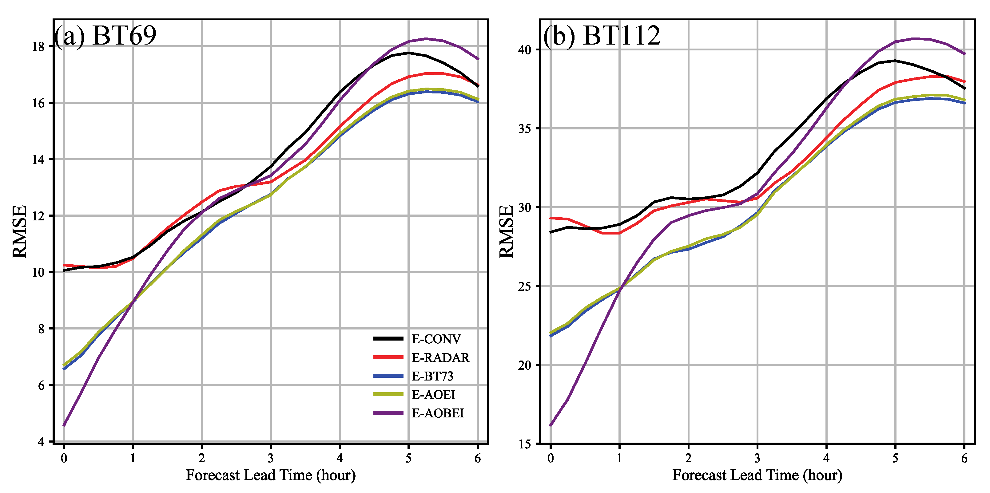
The second (third) column of Figure 6 shows that the forecasted BT69 ensemble means from the five experiments all become less (much less) close to the observed one in Figure 6b (c) as the forecast lead time increases to 3 (6) h. At 3 h forecast lead time, the forecasted ensemble means from E-BT73 and E-AOEI are still very close to each other and still closer to the observed one than that from E-RADAR, while the forecasted ensemble mean from E-AOBEI becomes slightly less close to the observed one than that from E-RADAR but still closer to the observed one than that from E-CONV. At 6 h forecast lead time, the forecasted ensemble means from E-BT73 and E-AOEI are still very close to each other and closer to the observed one than that from E-RADAR, while the forecasted ensemble mean from E-AOBEI becomes even less close to the observed one than that from E-CONV. The above comparisons are confirmed quantitatively by the RMSE of the forecasted BT69 ensemble mean plotted in Figure 7a as a function of the forecast lead time for each experiment in the first group.
BT112 observations are also used as ground truths to verify the forecasted BT112 ensemble means at 0, 3, and 6 h forecast lead times valid at 2100 UTC, 0000, and 0300 UTC the next day, respectively, from each experiment in the first group. The comparisons are very similar to those illustrated for BT69 in Figure 6 (and thus omitted here), and they are confirmed quantitatively by the RMSE of the forecasted BT112 ensemble mean plotted in Figure 7b as a function of the forecast lead time for each experiment in the first group. Since BT69 (BT112) is not assimilated but can be used to diagnose mid-level troposphere water vapor (discrete clouds), the forecasted BT69 and BT112 can be used together as an indirect indication of cloud cover. Based on this understanding, the results in Figure 6 and Figure 7 indicate indirectly that assimilating reflectivity observations improves the cloud cover forecast slightly after 3 h forecast lead time, assimilating BT73 improves the cloud cover forecast significantly up to 6 h, but the forecast is not much affected by using AOEI, while using AOBEI improves (degrades) the cloud cover forecast before (after) 1 h forecast lead time.
4.3. Assimilation Statistics for the Second Group of Experiments
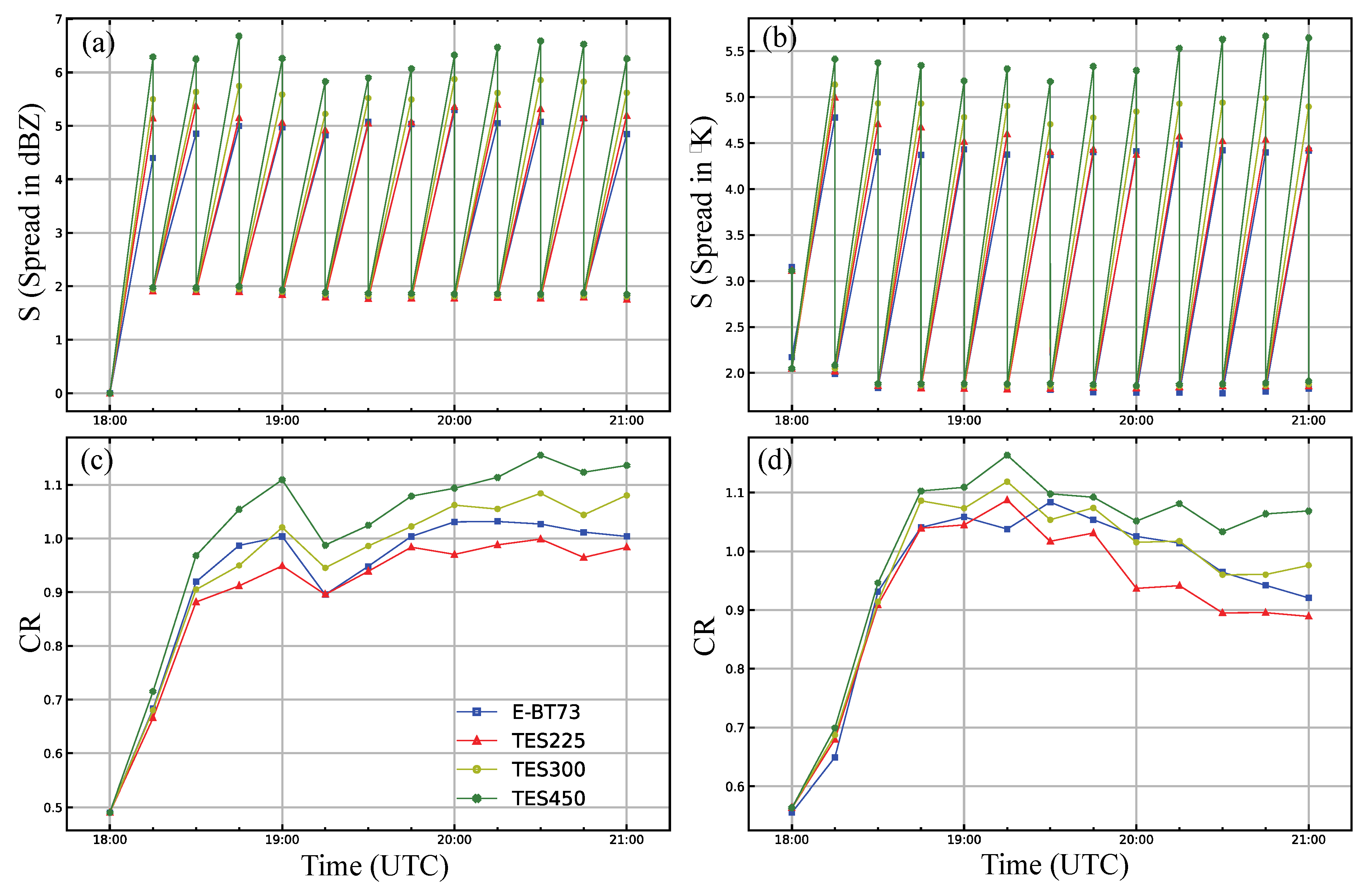
The ensemble spreads calculated for reflectivity (BT73) from the four experiments in the second group are shown in Figure 8a (b). As shown for either reflectivity or BT73, the posterior ensemble spreads from the three TES experiments are all very close to that from E-BT73, but the prior ensemble spreads from the three TES experiments become increasingly higher, from slightly higher to moderately higher, than that from E-BT73, as the shifting time interval τ increases successively from 225 to 300 and then to 450 s. Clearly, increasing τ enlarges the differences between the 12 ensemble members sampled at the analysis time and the 24 members sampled at the time levels sampled by ±τ. This explains why the prior ensemble spread increases as τ increases. The posterior ensemble spread, however, is not much affected by the increase of τ, indicating that all three TES experiments have about the same effectiveness in ensemble analyses as E-BT73.
The CRs calculated for reflectivity (BT73) from the four experiments in the second group are shown in Figure 8c (d). As shown for either reflectivity or BT73, the CR from TES300 is not only closer to that from E-BT73 but also closer to 1 than those from TES225 and TES450, while the CR from TES225 (TES450) is slightly lower (higher) than that from E-BT73 after the third assimilation cycle. Thus, TES300 has about the same assimilation statistics as E-BT73 and slightly better assimilation statistics than TES225 and TES450, although the assimilation statistics are not very sensitive to τ (specified within the range from 225 to 450 s).
4.4. Forecast Performances for the Second Group of Experiments
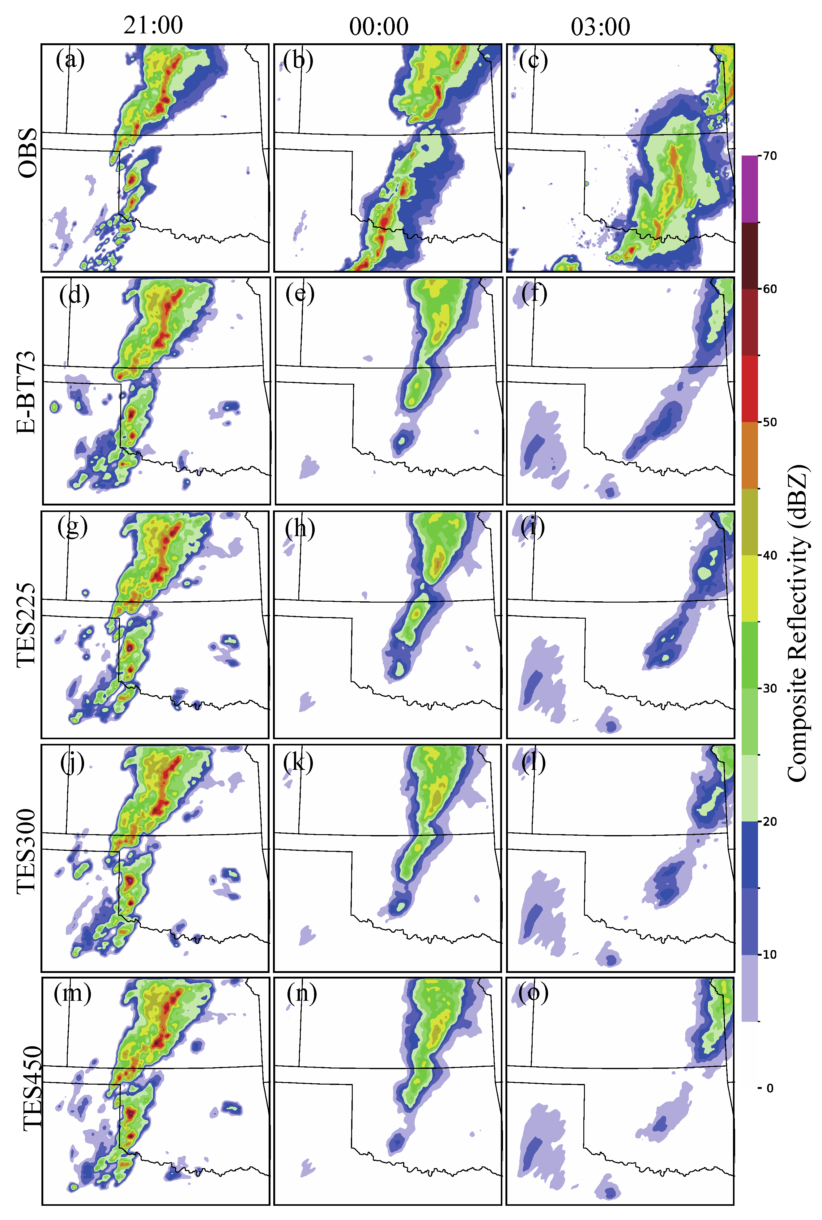
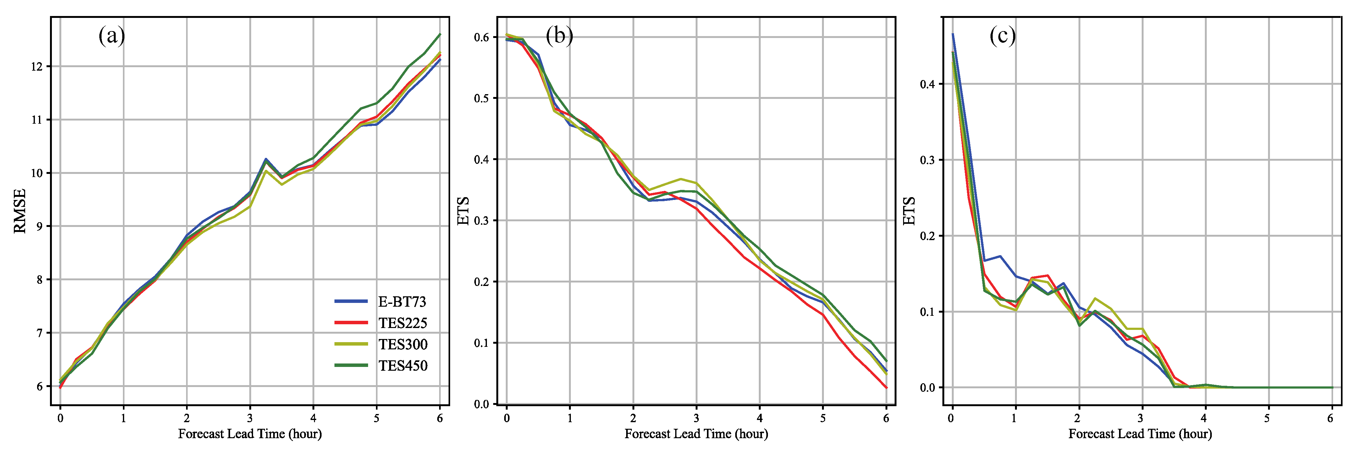
The composite reflectivity observations and the forecasted composite reflectivity ensemble means from E-BT73 in the first two rows of Figure 4 are duplicated in the first two rows of Figure 9 to compare with the forecasted composite reflectivity ensemble means (at 0, 3, and 6 h forecast lead times valid at 2100 UTC, 0000, and 0300 UTC the next day, respectively) from each TES experiment in each subsequent row of Figure 9. As shown in the first column of Figure 9, the 0 h forecasted composite reflectivity ensemble means from the three TES experiments are all very close to those from E-BT73 and also very close to the observed one. The second (third) column of Figure 9 shows that the forecasted composite reflectivity ensemble means from the three TES experiments are still very close to those from E-BT73, although the latter becomes less (much less) close to those observed in Figure 9b (c) as the forecast lead time increases to 3 (6) h. The above comparisons are confirmed quantitatively by the RMSE of the forecasted composite reflectivity ensemble mean plotted in Figure 10a as a function of the forecast lead time for each experiment in the second group. As shown in Figure 10a, the RMSEs from the three TES experiments are all very close to those from E-BT73, while the RMSE from TES300 is slightly smaller than that from E-BT73 between 2 and 5 h forecast lead times, and the RMSE from TES225 (TES450) is slightly larger than that from E-BT73 after 4 (5) h forecast lead time.
The ETSs of forecasted composite reflectivity ensemble means calculated using 20 and 40 dBZ thresholds from the three TES experiments are plotted as functions of forecast lead time against that from E-BT73 in Figure 10b,c, respectively. Figure 10b shows that the ETSs calculated using the 20 dBZ threshold from the three TES experiments are all very close to those from E-BT73, while the ETS from TES300 (TES450) is higher (slightly higher) than those from E-BT73 around 3 h forecast lead time (after 2 h forecast lead time). Figure 10c shows that the ETSs calculated using the 40 dBZ threshold from the three TES experiments are also very close to that from E-BT73 during most forecast lead times except between 0.5 and 1 h forecast lead times, while the ETS from TES300 (TES22, TES450) is higher (slightly higher) than that from E-BT73 after 2 h forecast lead time. The above results indicate that, in addition to reducing the computational cost, TES can also slightly improve the forecast by optimally selecting τ, although the forecast accuracy and quality are not very sensitive to τ (selected between 225 and 450 s).
5. Conclusions
In this paper, by using the convection-allowing ensemble-based Warn-on-Forecast System (WoFS), two groups of experiments are designed and performed to assimilate all-sky infrared Brightness Temperature (BT) observations from the GOES-16 7.3 μm low-level troposphere water vapor channel (BT73) in combination with radar wind and reflectivity observations, in addition to conventional observations (from the Oklahoma Mesonet), for the severe storm event that occurred in Oklahoma on 2 May 2018. Radar reflectivity observations and BT observations from the GOES-16 6.9 μm mid-level troposphere water vapor channel and 11.2 μm longwave window channel are used to evaluate the assimilation statistics and verify the forecasts in each experiment. The first group contains one control experiment (which assimilates only conventional observations) and four impact-test experiments (see Table 2). The first impact-test experiment, named E-RADAR, assimilates radar reflectivity and radial-velocity observations in addition to conventional observations; the second impact-test experiment, named E-BT73, assimilates all-sky BT73 observations, based primarily on the previous studies [7,8], in addition to those assimilated in E-RADAR; and the third (fourth) impact-test experiment assimilates the same observations as those assimilated in E-BT73 but uses the adaptive observation error inflation, AOEI [11] (plus the adaptive background error inflation, ABEI [12]). The results from these experiments are summarized below:
(i) Assimilating BT73 (without using ABEI) in addition to radar data slightly improves the ensemble estimated background error variance for reflectivity but does not much affect the reflectivity forecast, and the estimated error variance is not much affected by the use of AOEI but degraded slightly by the use of ABEI.
(ii) Assimilating reflectivity observations improves the overall precipitation forecast up to 5 h, and further assimilating BT73 slightly degrades (improves) the forecast before (after) 3 h forecast lead time, while using AOEI, AOBI, or both does not much affect the forecast.
(iii) Assimilating reflectivity observations improves heavy precipitation forecasts nearly up to 4 h, and further assimilating BT73 slightly improves the forecast only between 1 h and 3 h forecast lead times, while using AOEI does not much affect the forecast and using AOBI does not improve the forecast until the forecast lead time increases beyond 3 h.
(iv) Assimilating reflectivity observations improves the cloud cover forecast slightly after 3 h forecast lead time, assimilating BT73 improves the cloud cover forecast significantly up to 6 h, but the forecast is not much affected by using AOEI, while using ABEI improves (degrades) the cloud cover forecast before (after) 1 h forecast lead time.
The second group contains one control experiment (which is taken from E-BT73 in the first group) and three TES experiments (see Table 3). The three TES experiments apply time-expanded sampling (TES) to E-BT73, with the time interval for expanded sampling set to τ = 225, 300, and 450 s, respectively. The results from these experiments are summarized below:
(i) Increasing τ can increase the prior ensemble spread but not much affect the posterior ensemble spread, and the assimilation statistics can be slightly improved by optimally selecting τ (around 300 s).
(ii) TES can slightly improve the forecast by optimally selecting τ, although the forecast accuracy and quality are not very sensitive to τ (selected between 225 and 450 s).
The summarized results suggest that TES is appealing and useful for cost-saving real-time applications to WoFS in assimilating all-sky BT73 observations in combination with radar wind and reflectivity observations and generating short-term severe weather forecasts. For data assimilation cycles, model integration for each updating run in E-BT73 takes 2 cores with the NSSL supercomputer. It totally took 36 × 2 = 72 cores for ensemble model integration during one data assimilation window. TES reduces the number of updating runs to 1/3 of that in E-BT73 and thus reduces the number of cores from 72 used in E-BT73 to only 12 × 2 = 24. Note that the integration time for each updating run in the TES experiment with τ = 300 s = T/3 (where T = 15 min is the assimilation cycle time interval) is increased from T in E-BT73 to 4T/3, so the computational cost for data assimilation cycles in the TES experiment is 4/9 of the cost in E-BT73, and this saves 5/9 of the computational cost. Thus, TES can not only slightly improve the forecast but also reduce the computational cost.
The insensitivity of the assimilation statistics and subsequent forecast to τ is attractive for real-time applications because labor-intensive adaptive tuning and/or cumbersome event-based selection of τ may be avoided or skipped in preparing TES for future real-time applications with the WoFS, although continued research is required on using TES to improve remote sensing data assimilations (including all-sky BT data assimilation) and subsequent forecasts of severe storms.
Finally, it is necessary to mention that in addition to the 2 May 2018 severe weather event tested in this paper, the WoFS has also been applied to two more severe weather events that occurred on 8 May 2019 in Texas and on 30 April 2018 in Nebraska for assimilating all-sky BT73 in combination with radar observations to improve the analysis and subsequent forecast of severe thunderstorms. Similar impact-test experiments were performed for these two additional severe weather events, and their results also support the primary findings presented and summarized in this paper.
Author Contributions
Experiment design and execution, EnKF code modifications, evaluations of experiment results, manuscript preparation, visualization, and writing—review/revision: H.Z. Writing original draft and review/revision, supervision, and funding acquisition: Q.X. Observational data and EnKF code preparations, and writing—review/revision: T.A.J. Manuscript review/revision, project administration, and funding acquisition: L.R. All authors have read and agreed to the published version of the manuscript.
Funding
The research work was supported by the NSSL Warn-on-Forecast project, the Office of Naval Research under Award Number N000142012449 to the University of Oklahoma (OU), and the National Natural Science Foundation of China Grant 42275010 to the Institute of Atmospheric Physics. Funding was also provided by NOAA/Office of Oceanic and Atmospheric Research under NOAA-OU Cooperative Agreement #NA21OAR4320204, U.S. Department of Commerce.
Acknowledgments
The authors are thankful to Jidong Gao at NSSL and the three anonymous reviewers for providing constructive comments and suggestions.
Conflicts of Interest
The authors have declared that no competing interests exist.
References
- Derber, J.C.; Wu, W.-S. The Use of TOVS Cloud-Cleared Radiances in the NCEP SSI Analysis System. Mon. Weather Rev. 1998, 126, 2287–2299. [Google Scholar] [CrossRef]
- McNally, A.P.; Watts, P.D.; Smith, J.A.; Engelen, R.; Kelly, G.A.; Thépaut, J.N.; Matricardi, M. The Assimilation of AIRS Radiance Data at ECMWF. Q. J. R. Meteorol. Soc. 2006, 132, 935–957. [Google Scholar] [CrossRef] [Green Version]
- Zhu, Y.; Liu, E.; Mahajan, R.; Thomas, C.; Groff, D.; Van Delst, P.; Collard, A.; Kleist, D.; Treadon, R.; Derber, J.C. All-Sky Microwave Radiance Assimilation in NCEP’s GSI Analysis System. Mon. Weather Rev. 2016, 144, 4709–4735. [Google Scholar] [CrossRef]
- Schmit, T.J.; Gunshor, M.M.; Menzel, W.P.; Gurka, J.J.; Li, J.; Bachmeier, A.S. Introducing the next-generation Advanced Baseline Imager on GOES-R. Bull. Am. Meteorol. Soc. 2005, 86, 1079–1096. [Google Scholar] [CrossRef]
- Wheatley, D.M.; Knopfmeier, K.H.; Jones, T.A.; Creager, G.J. Storm-Scale Data Assimilation and Ensemble Forecasting with the NSSL Experimental Warn-on-Forecast System. Part I: Radar Data Experiments. Weather Forecast. 2015, 30, 1795–1817. [Google Scholar] [CrossRef]
- Jones, T.A.; Knopfmeier, K.; Wheatley, D.; Creager, G.; Minnis, P.; Palikonda, R. Storm-Scale Data Assimilation and Ensemble Forecasting with the NSSL Experimental Warn-on-Forecast System. Part II: Combined Radar and Satellite Data Experiments. Weather Forecast. 2016, 31, 297–327. [Google Scholar] [CrossRef]
- Jones, T.A.; Wang, X.; Skinner, P.; Johnson, A.; Wang, Y. Assimilation of GOES-13 Imager Clear-Sky Water Vapor (6.5 mm) Radiances into a Warn-on-Forecast System. Mon. Weather Rev. 2018, 146, 1077–1107. [Google Scholar] [CrossRef]
- Jones, T.A.; Skinner, P.; Yussouf, N.; Knopfmeier, K.; Reinhart, A.; Wang, X.; Bedka, K.; Smith, W.; Palikonda, R. Assimilation of GOES-16 Radiances and Retrievals into the Warn-on-Forecast System. Mon. Weather Rev. 2020, 148, 1829–1859. [Google Scholar] [CrossRef]
- Zhang, Y.; Stensrud, D.J.; Zhang, F. Simultaneous Assimilation of Radar and All-Sky Satellite Infrared Radiance Observations for Convection-Allowing Ensemble Analysis and Prediction of Severe Thunderstorms. Mon. Weather Rev. 2019, 147, 4389–4409. [Google Scholar] [CrossRef]
- Zhang, Y.; Zhang, F.; Stensrud, D.J. Assimilating All-Sky Infrared Radiances from GOES-16 ABI Using an Ensemble Kalman Filter for Convection-Allowing Severe Thunderstorms Prediction. Mon. Weather Rev. 2018, 146, 3363–3381. [Google Scholar] [CrossRef]
- Minamide, M.; Zhang, F. Adaptive Observation Error Inflation for Assimilating All-Sky Satellite Radiance. Mon. Weather Rev. 2017, 145, 1063–1081. [Google Scholar] [CrossRef] [Green Version]
- Minamide, M.; Zhang, F. An Adaptive Background Error Inflation Method for Assimilating All-Sky Radiances. Q. J. R. Meteorol. Soc. 2019, 145, 805–823. [Google Scholar] [CrossRef]
- Xu, Q.; Wei, L.; Lu, H.; Qiu, C.; Zhao, Q. Time-Expanded Sampling for Ensemble-Based Filters: Assimilation Experiments with a Shallow-Water Equation Model. J. Geophys. Res. Atmos. 2008, 113, D02114. [Google Scholar] [CrossRef]
- Xu, Q.; Lu, H.; Gao, S.; Xue, M.; Tong, M. Time-Expanded Sampling for Ensemble Kalman Filter: Assimilation Experiments with Simulated Radar Observations. Mon. Weather Rev. 2008, 136, 2651–2667. [Google Scholar] [CrossRef] [Green Version]
- Huang, B.; Wang, X. On the Use of Cost-Effective Valid-Time-Shifting (VTS) Method to Increase Ensemble Size in the GFS Hybrid 4DEnVar System. Mon. Weather Rev. 2018, 146, 2973–2998. [Google Scholar] [CrossRef]
- Gasperoni, N.A.; Wang, X.; Wang, Y. Using a Cost-Effective Approach to Increase Background Ensemble Member Size within the GSI-Based EnVar System for Improved Radar Analyses and Forecasts of Convective Systems. Mon. Weather Rev. 2022, 150, 667–689. [Google Scholar] [CrossRef]
- Lu, H.; Xu, Q.; Yao, M.; Gao, S. Time-Expanded Sampling for Ensemble-Based Filters: Assimilation Experiments with Real Radar Observations. Adv. Atmos. Sci. 2011, 28, 743–757. [Google Scholar] [CrossRef]
- Zhao, Q.; Xu, Q.; Jin, Y.; McLay, J.; Reynolds, C. Time-Expanded Sampling for Ensemble-Based Data Assimilation Applied to Conventional and Satellite Observations. Weather Forecast. 2015, 30, 855–872. [Google Scholar] [CrossRef] [Green Version]
- Zhang, H.; Gao, J.; Xu, Q.; Ran, L. Applying Time-Expended Sampling to Ensemble Assimilation of Remote Sensing Data for Short-Term Predictions of Thunderstorms. Remote Sens. 2023, 15, 2358. [Google Scholar] [CrossRef]
- Skamarock, W.C.; Klemp, J.B.; Dudhia, J.; Gill, D.O.; Barker, D.M.; Duda, M.G.; Huang, X.-Y.; Wang, W.; Powers, J.G. A Description of the Advanced Research WRF Version 3; National Center for Atmospheric Research, Mesoscale and Microscale Meteorology Division: Boulder, CO, USA, 2008.
- Liu, H.; Hu, M.; Ge, G.; Zhou, C.; Stark, D.; Shao, H.; Newman, K.; Whitaker, J. Ensemble Kalman Filter (EnKF). In User’s Guide Version 1.3-Compatible with GSI Community Release v3.7; NOAA/OAR/Global Systems Laboratory, Developmental Testbed Center: Boulder, CO, USA, 2018; Available online: https://dtcenter.org/community-code/ensemble-kalman-filter-system-enkf/documentation (accessed on 25 April 2023).
- Weng, F. Advances in Radiative Transfer Modeling in Support of Satellite Data Assimilation. J. Atmos. Sci. 2007, 64, 3799–3807. [Google Scholar] [CrossRef]
- Whitaker, J.S.; Hamill, T.M.; Wei, X.; Song, Y.; Toth, Z. Ensemble Data Assimilation with the NCEP Global Forecast System. Mon. Weather Rev. 2008, 136, 463–482. [Google Scholar] [CrossRef] [Green Version]
- Benjamin, S.G.; Weygandt, S.S.; Brown, J.M.; Hu, M.; Alexander, C.R.; Smirnova, T.G.; Olson, J.B.; James, E.P.; Dowell, D.C.; Grell, G.A.; et al. A North American Hourly Assimilation and Model Forecast Cycle: The Rapid Refresh. Mon. Weather Rev. 2016, 144, 1669–1694. [Google Scholar] [CrossRef]
- Mansell, E.R.; Ziegler, C.L.; Bruning, E.C. Simulated Electrification of a Small Thunderstorm with Two-Moment Bulk Microphysics. J. Atmos. Sci. 2010, 67, 171–194. [Google Scholar] [CrossRef]
- Gaspari, G.; Cohn, S.E. Construction of Correlation Functions in Two and Three Dimensions. Q. J. R. Meteorol. Soc. 1999, 125, 723–757. [Google Scholar] [CrossRef]
- Zhang, J.; Howard, K.; Langston, C.; Kaney, B.; Qi, Y.; Tang, L.; Grams, H.; Wang, Y.; Cockcks, S.; Martinaitis, S.; et al. Multi-Radar Multi-Sensor (MRMS) Quantitative Precipitation Estimation: Initial Operating Capabilities. Bull. Am. Meteorol. Soc. 2016, 97, 621–638. [Google Scholar] [CrossRef]
- Smith, T.M.; Lakshmanan, V.; Stumpf, G.J.; Ortega, K.L.; Hondl, K.; Cooooper, K.; Calhoun, K.M.; Kingfield, D.M.; Manrossossoss, K.L.; Toooomey, R.; et al. Multi-Radar Multi-Sensor (MRMS) Severe Weather and Aviation Products: Initial Operating Capabilities. Bull. Am. Meteorol. Soc. 2016, 97, 1617–1630. [Google Scholar] [CrossRef]
- Dowell, D.C.; Wicker, L.J. Additive Noise for Storm-Scale Ensemble Data Assimilation. J. Atmos. Ocean. Technol. 2009, 26, 911–927. [Google Scholar] [CrossRef] [Green Version]
- Wilks, D.S. Statistical Methods in the Atmospheric Sciences, 3rd ed.; International Geophysics Series; Academic Press: Cambridge, MA, USA, 2011; Volume 100, 704p. [Google Scholar]
Figure 1.
(a) Timeline of EnKF data assimilation cycles used with the WoFS (without TES). (b) As in (a), but with TES.
Figure 1.
(a) Timeline of EnKF data assimilation cycles used with the WoFS (without TES). (b) As in (a), but with TES.

Figure 2.
(a) Surface analysis map at 1800 UTC on 2 May 2018 over WoFS domain and surrounding areas. (b) Model domain, terrain height plotted by color shades, and locations of tornadoes, hail, and damaging winds (occurred during the time period from 1800 UTC to 0300 UTC the next day according to local storm reports issued from the National Weather Service) plotted by red triangles, green dots, and blue squares, respectively, for the 2 May 2018 severe storm event. (c) Radar composite reflectivity (shown by color shades) at 1800 UTC on 2 May 2018 over model domain. (d) As in (c), but at 2100 UTC. (e) As in (c), but for GOES-16 visible, (6.4 μm) image from band 2 (shown by gray shades) and infrared BT from band 13 at 10.3 μm wavelength (shown by color shades). (f) As in (e), but at 2100 UTC.

Figure 3.
(a) Reflectivity ensemble spreads from the four impact-test experiments plotted by zig-zag curves of different colors as functions of time (from 1800 to 2100 UTC). (b) As in (a), but for BT73 ensemble spreads from the last three impact-test experiments. (c) As in (a), but for reflectivity CRs. (d) As in (c), but for BT73 CRs. The four curves in panel (a) largely coincide. The blue and yellow curves in panel (a) also largely coincide. On each curve in panel (a) or (b), each abrupt drop associated with a zig-zag jump shows how a prior spread is sharply reduced to a posterior spread immediately after the analysis time in each assimilation cycle.

Figure 4.
(a–c) Observed composite reflectivity plotted by color shades valid at 2100 UTC, 0000, and 0300 UTC, respectively, for the 2 May 2018 severe weather event. (d–f) As in (a–c), but for ensemble means of 0, 3, and 6 h forecasted composite reflectivity from E-CONV. (g–i) As in (d–f), but from E-RADAR. (j–l) As in (d–f), but from E-BT73. (m–o) As in (d–f), but from E-AOEI. (p–r) As in (d–f), but from E-AOBEI.

Figure 5.
(a) RMSEs of forecasted composite reflectivity ensemble means from the five experiments in the first group (verified against MRMS products) plotted by five differently colored curves as functions of forecast lead time. (b) ETSs of forecasted composite reflectivity ensemble means calculated by using 20 dBZ threshold from the five experiments in the first group and plotted by five differently colored curves as functions of forecast lead time. (c) As in (b), but calculated by using 40 dBZ threshold.

Figure 6.
As in Figure 4, but for BT69.
Figure 6.
As in Figure 4, but for BT69.

Figure 7.
(a) RMSEs of forecasted BT ensemble means at 6.9 μm wavelength (BT69). (b) RMSEs of forecasted BT ensemble means at 11.2 μm wavelength (BT112).
Figure 7.
(a) RMSEs of forecasted BT ensemble means at 6.9 μm wavelength (BT69). (b) RMSEs of forecasted BT ensemble means at 11.2 μm wavelength (BT112).

Figure 8.
As in Figure 3, but for the four experiments in the second group.
Figure 8.
As in Figure 3, but for the four experiments in the second group.

Figure 9.
As in Figure 4, but for the four experiments in the second group.
Figure 9.
As in Figure 4, but for the four experiments in the second group.

Figure 10.
As in Figure 5, but for the four experiments in the second group.
Figure 10.
As in Figure 5, but for the four experiments in the second group.


Table 1.
Observation error standard deviations (SDs), horizontal localization (HL) radii, and vertical localization (VL) depths for all observation types assimilated into WoFS in this study, where p denotes the vertical level in pressure and po = 1000 hPa.
Table 1.
Observation error standard deviations (SDs), horizontal localization (HL) radii, and vertical localization (VL) depths for all observation types assimilated into WoFS in this study, where p denotes the vertical level in pressure and po = 1000 hPa.
| Observation | Error SD | HL Radius in km | VL Depth in ln(po/p) |
|---|---|---|---|
| Temperature | 1.5 (K) | 60 | 0.85 |
| Dewpoint | 2.0 (K) | 60 | 0.85 |
| U wind | 1.75 (m/s) | 60 | 0.85 |
| V wind | 1.75 (m/s) | 60 | 0.85 |
| Pressure | 1.0 hPa | 60 | 0.85 |
| Reflectivity | 7 (dBZ) | 18 | 0.8 |
| Radial velocity | 3 (m/s) | 18 | 0.8 |
| BT73-clear | 1.75 (K) | 36 | 4.0 |
| BT73-cloudy | 3.5 (K) | 36 | 4.0 |
Table 2.
Experiments designed in the first group.
| Experiment Name | Description | ||
|---|---|---|---|
| Assimilated Obs. | Obs. Error SD of TB73 | Inflation | |
| E-CONV | Conventional obs. (from Oklahoma Mesonet) | RTPS: 0.9 | |
| E-RADAR | Conv + Radar (reflectivity and radial wind) | RTPS: 0.9 | |
| E-BT73 | Conv + Radar + TB73 | Clear-sky: 1.75 K Cloudy-sky: 3.5 K | RTPS: 0.9 |
| E-AOEI | Conv + Radar + TB73 | AOEI | RTPS: 0.9 |
| E-AOBEI | Conv + Radar + TB73 | AOEI | ABEI + RTPS: 0.9 |
Table 3.
Configurations of experiments in the second group, where Ns is the ensemble size used in assimilation updating runs.
Table 3.
Configurations of experiments in the second group, where Ns is the ensemble size used in assimilation updating runs.
| Experiment Name | Description |
|---|---|
| E-BT73 | Ns = 36 without TES |
| TES225 | Ns = 12 with TES and τ = 225 s |
| TES300 | Ns = 12 with TES and τ = 300 s |
| TES450 | Ns = 12 with TES and τ = 450 s |
Disclaimer/Publisher’s Note: The statements, opinions and data contained in all publications are solely those of the individual author(s) and contributor(s) and not of MDPI and/or the editor(s). MDPI and/or the editor(s) disclaim responsibility for any injury to people or property resulting from any ideas, methods, instructions or products referred to in the content. |
© 2023 by the authors. Licensee MDPI, Basel, Switzerland. This article is an open access article distributed under the terms and conditions of the Creative Commons Attribution (CC BY) license (https://creativecommons.org/licenses/by/4.0/).
Share and Cite
MDPI and ACS Style
Zhang, H.; Xu, Q.; Jones, T.A.; Ran, L. Assimilating All-Sky Infrared Radiance Observations to Improve Ensemble Analyses and Short-Term Predictions of Thunderstorms. Remote Sens. 2023, 15, 2998. https://doi.org/10.3390/rs15122998
AMA Style
Zhang H, Xu Q, Jones TA, Ran L. Assimilating All-Sky Infrared Radiance Observations to Improve Ensemble Analyses and Short-Term Predictions of Thunderstorms. Remote Sensing. 2023; 15(12):2998. https://doi.org/10.3390/rs15122998
Chicago/Turabian StyleZhang, Huanhuan, Qin Xu, Thomas A. Jones, and Lingkun Ran. 2023. "Assimilating All-Sky Infrared Radiance Observations to Improve Ensemble Analyses and Short-Term Predictions of Thunderstorms" Remote Sensing 15, no. 12: 2998. https://doi.org/10.3390/rs15122998
Note that from the first issue of 2016, this journal uses article numbers instead of page numbers. See further details here.