

Observed Surface Wind Field Structure of Severe Tropical Cyclones and Associated Precipitation

1
Department of Atmospheric and Oceanic Sciences & Institute of Atmospheric Sciences, Fudan University, Shanghai 200433, China
2
School of Marine Sciences, Nanjing University of Information Science & Technology, Nanjing 210044, China
3
National Meteorological Center, Beijing 100081, China
*
Author to whom correspondence should be addressed.
Remote Sens. 2023, 15(11), 2808; https://doi.org/10.3390/rs15112808
Submission received: 29 March 2023
/
Revised: 21 May 2023
/
Accepted: 22 May 2023
/
Published: 29 May 2023
(This article belongs to the Special Issue Remote Sensing and Parameterization of Air-Sea Interaction)
Abstract
:Using the International Best Track Archive for Climate Stewardship (IBTrACS) dataset, this study assessed the surface wind fields from high spatial resolution Synthetic Aperture Radar (SAR) observations, the fifth generation ECMWF reanalysis for the global climate and weather (ERA5) data and the Tropical Cyclone Winds and Inflow Angle Asymmetry (TCIAA) wind model. The results showed that SAR data are sufficient to reveal the surface wind field near a TC center and can accurately describe TC intensity and size under severe TC conditions. Then, a new, improved statistical wind structure model was set up using ERA5 data alone based on the assessment. In addition, the warm sea surface (SST > 26.5 °C) produced stronger TC wind fields and heavier precipitation. When the SST was higher (lower), the heavy rainfall was located on the left (right) side of the TC track and the strong positive correlation between wind speed and precipitation increased as the SST decreased.

1. Introduction
A tropical cyclone (TC) is a cyclonic vortex with a warm core structure that usually originates over warm tropical oceans. TCs are one of the most damaging natural disasters in the world. TCs always bring heavy rainfall, gale force winds and large storm surges that can lead to urban waterlogging, flooding and property damage and can threaten the lives of coastal residents [1,2]. Taking China as an example, the direct economic losses resulting from TCs were estimated to be 6 billion dollars per year and these losses have increased significantly in recent decades [3]. Both theoretical studies and model simulations indicate that both the intensity of TCs and the frequency of more severe TCs are increasing as the global temperature rises [4,5,6,7]. As a result, global warming will lead to an increase in the TC destructiveness [6,8]. Further, because coastal populations continue to increase, there is a growing probability of a substantial increase in TC-related loss of life and property [9].
In order to reduce the losses caused by TCs, better TC prediction and warning is of extreme importance. To improve our predictive ability regarding TCs, the two following aspects are useful: the first is to improve the description of the TC structure and intensity, and the second is to obtain a more accurate and reliable ocean initial field, both of which can improve the simulation of air–sea interactions under TC conditions [10,11]. Both of these require improving the accuracy of the TC wind field model [12].
The early empirical models, such as the Batts model, were built based on probabilistic models which were first developed by Russell [13]. These empirical models were based on both the climatological characteristics of TCs in a specific ocean basin, and Monte Carlo simulation [14]. Although the empirical models are easy to follow, their results are strongly ocean-basin dependent. Then, developed empirical models such as the Holland model were built to add the atmospheric pressure field into the gradient wind equation to describe the wind profile and physical parameters of the TCs better [15]. However, the Holland model needs accurate observations and an empirical relationship between pressure profile and radius, both of which are difficult to obtain. Some wind field models, such as the Shapiro model [16] and the Yan Meng model [17], were also built up by solving the momentum equations and assuming a constant boundary layer depth. Due to the lack of observational data over the last century, these wind field models can still be refined to better match the structure of a TC. With an increase in higher resolution data, such as Multiplatform Tropical Cyclone Surface Wind Analysis (MTCSWA) and buoy observations, new statistical models have advanced. For example, there are now symmetric wind field models [18], an inflow angle asymmetry model (TCIAA model) [19], a decomposed TC boundary layer model [20,21], and a height-resolving, linear analytical model of the boundary layer [22]. These newly developed models provide a relatively accurate description of the entire surface wind field of a TC.
To better describe the TC wind structure, an understanding of the interaction between TCs and the upper ocean is also important. TCs typically cause a severe disturbance in the upper ocean and create a cold wake, and strong TCs can induce more cooling. Conversely, the ocean also influences the intensity of TCs [11]; high Sea Surface Temperature (SST) over the path of a TC induces a stronger storm. In addition, TC precipitation that occurs over the ocean is not only associated with TC intensity, but also with SST through TC driven changes to the sensible heat flux and post-cyclone mixing depth [23,24,25]. However, the relationship between TC wind fields and SST is complicated and needs to be explored further.
Synthetic Aperture Radar (SAR) is an active observation system that has been installed on numerous platforms such as aircraft or satellites. Because of its high spatial resolution, large coverage area, and it being less affected by clouds, SAR has been widely used to measure atmospheric and oceanic phenomena [26]. For TC observation, the ocean surface wind vectors from combined co-polarized and cross-polarized SAR measurements have high spatial resolution with high accuracy for winds larger than 25 m/s under severe TC conditions [27]. Using the accurate SAR ocean surface wind fields, the reanalysis data and model simulated wind fields will be assessed and used to derive an improved statistical model of TC wind structure. In addition, the relationship among TC winds, SST and TC rainfall will also be addressed.
2. Data and Methods
2.1. Dataset
2.1.1. Synthetic Aperture Radar (SAR)
Wind speeds from dual-polarized SAR are used in the study. The dual-polarized SAR combined both co-polarized and cross-polarized channels to make a wind speed observation. The previous study showed that co-polarization (VV or HH) worked well under low to moderate wind speeds, but the sensitivity decreased at high wind speeds [28,29]. Although cross-polarization (VH or HV) exhibited improved sensitivity compared with co-polarization, the combination of both channels, i.e., the dual-polarized SAR, had quite high accuracy for wind speeds larger than 25 m/s [27]. The spatial resolution of the SAR wind field was also quite high and could reach to about 100 m. We obtained 121 data files from SAR for TCs. TCs that were located in the Eastern Pacific and files with missing values which led to incomplete TC coverage were deleted. As a result, the SAR dataset for this study included 44 different observation times for 28 different TCs observed in the Western North Pacific (WNP) between 2012 and 2020. The derived wind speeds in SAR data were averages over 2–3 min. During the calculation, all the wind speed data were interpolated onto a 0.05° × 0.05° grid.
2.1.2. International Best Track Archive for Climate Stewardship (IBTrACS)
IBTrACS provides the location and intensity for global tropical cyclones. The World Meteorological Organization Tropical Cyclone Programme has endorsed IBTrACS as the official archiving and distribution resource for the best track tropical cyclone data [30,31,32]. From the physical parameters provided by the Joint Typhoon Warning Center (JTWC) in the IBTrACS dataset, we chose the location, radius of maximum wind, minimum sea level pressure, pressure of the last closed isobar and the radius of 34 kt (about 17 m/s) wind speed in each of the four quadrants for the current study.
2.1.3. GPM_3IMERGHH
Half-hourly precipitation data at 0.1° × 0.1° spatial resolution were taken from the Global Precipitation Measurement (GPM) dataset that uses the Integrated Multi-satellitE Retrievals for GPM (IMERG) to calculate the precipitation from the observation of various precipitation-relevant satellites [33].
2.1.4. ERA5 Reanalysis Data
The hourly 10 m eastward (u) and westward (v) components of wind were taken from ERA5, which is the fifth generation ECMWF reanalysis of the global climate and weather for the past 4 to 7 decades. The spatial resolution of the ERA5 wind field is 0.25° × 0.25° [34].
2.1.5. COBE Sea Surface Temperature
The monthly COBE SST dataset with a spatial resolution of 1° × 1° was used in this study to characterize the upper ocean’s thermal state. COSE SST is also the input for the JMA Climate Data Assimilation System (JCDAS) and the Japanese 25-year Re-analyses (JRA-25 and JRA-55) [35].
2.2. Methods
2.2.1. Data Analysis and Statistical Methods
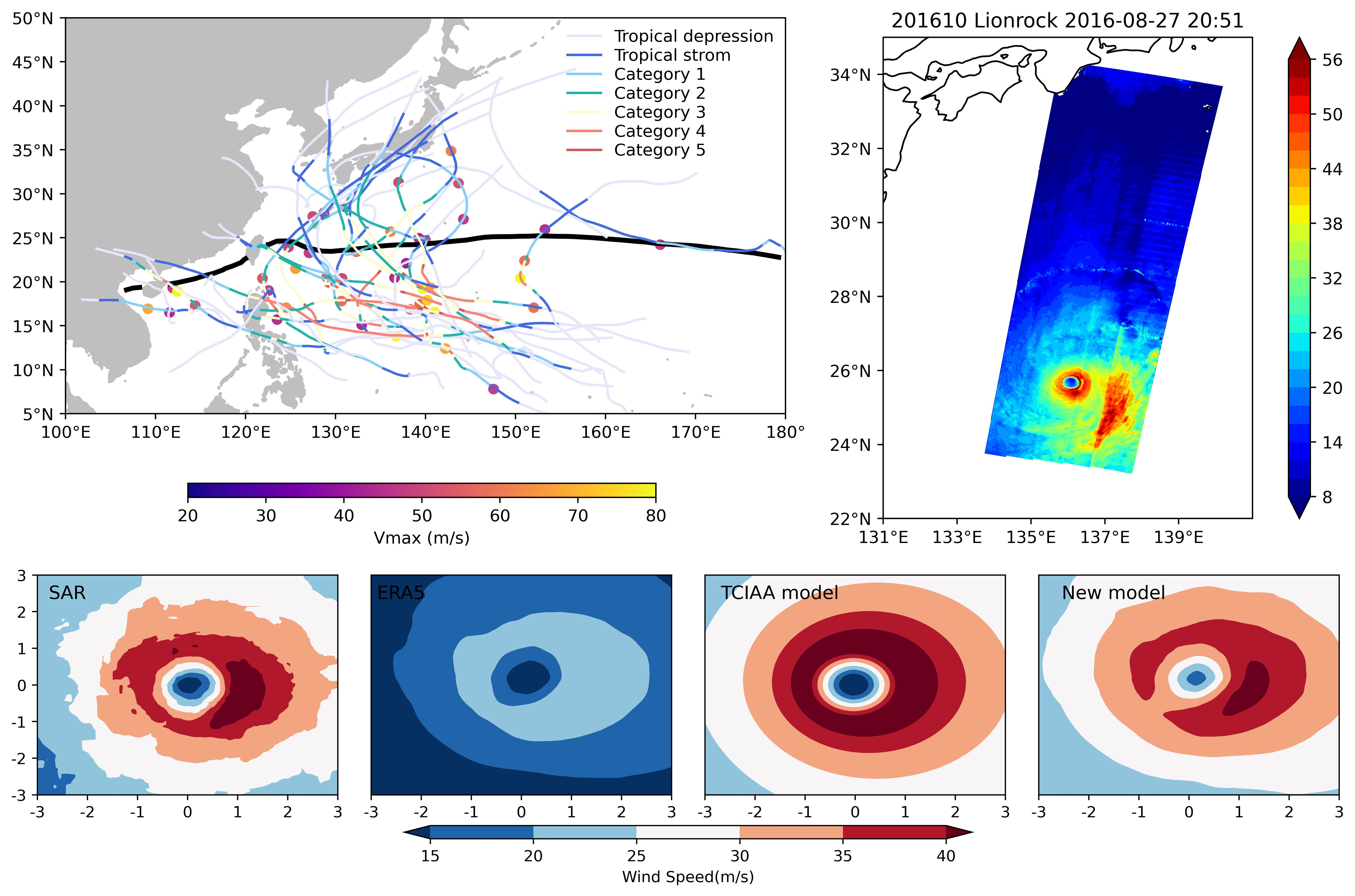
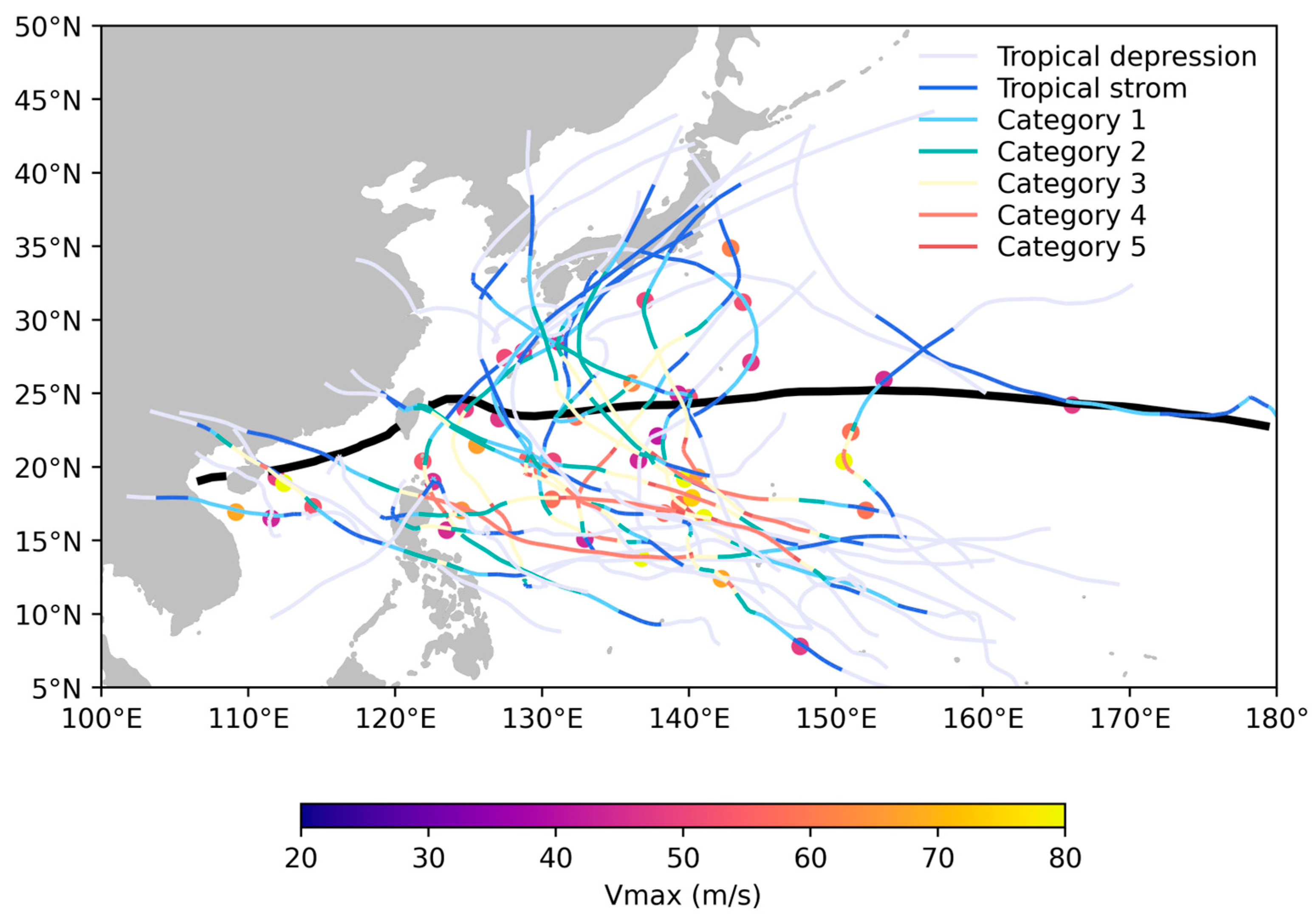
As described above, based on limitations in the data, 44 different severe TC observation times during 28 different TCs over the Western North Pacific Ocean were used in this study, and the tracks of those TCs are shown in Figure 1. The translation speed and direction of each TC can be estimated from the IBTrACS data. Wind speeds, longitude and latitude can be measured from SAR data, and the center location (location of the minimum wind speed in a TC center), the maximum wind speed, the Radius of Maximum Wind speed (RMW), which is the distance between the maximum wind speed and TC center, and the radius of gale-force wind of each TC were calculated. The wind field and precipitation data were interpolated onto a 0.05° × 0.05° grid for subsequent analysis and comparison.
2.2.2. TCIAA Model
The TCIAA (Tropical Cyclone Winds and Inflow Angle Asymmetry) model decomposes the SAR-derived winds into vortex rotational winds and a TC motion vector which represents the asymmetrical surface wind structure [19]. The TCIAA surface wind vector is obtained by superimposing the surface motion vector onto the rotation wind of a symmetric TC vector as:
where is based on the Rankine vortex and is a function of the maximum wind speed, RMW, and a fitting parameter, α, is the surface motion vector of the TC, and r and θ are the radial distance to the center and the angle to the east. In this paper, the RMW, maximum wind speed, α, and surface motion vector are assumed to be given initially, so the hypothesized TCIAA wind field structure is defined temporally. Then, by fitting the reconstructed wind field to the SAR surface wind field, the parameters RMW, max wind speed (), α, and surface wind motion vector () can be determined by the values where the standard deviation is the smallest and the correlation coefficient is the largest. Once these parameters have been obtained, the TCIAA wind speed field can be constructed from Equation (1).
3. Results
3.1. Wind Field Comparison
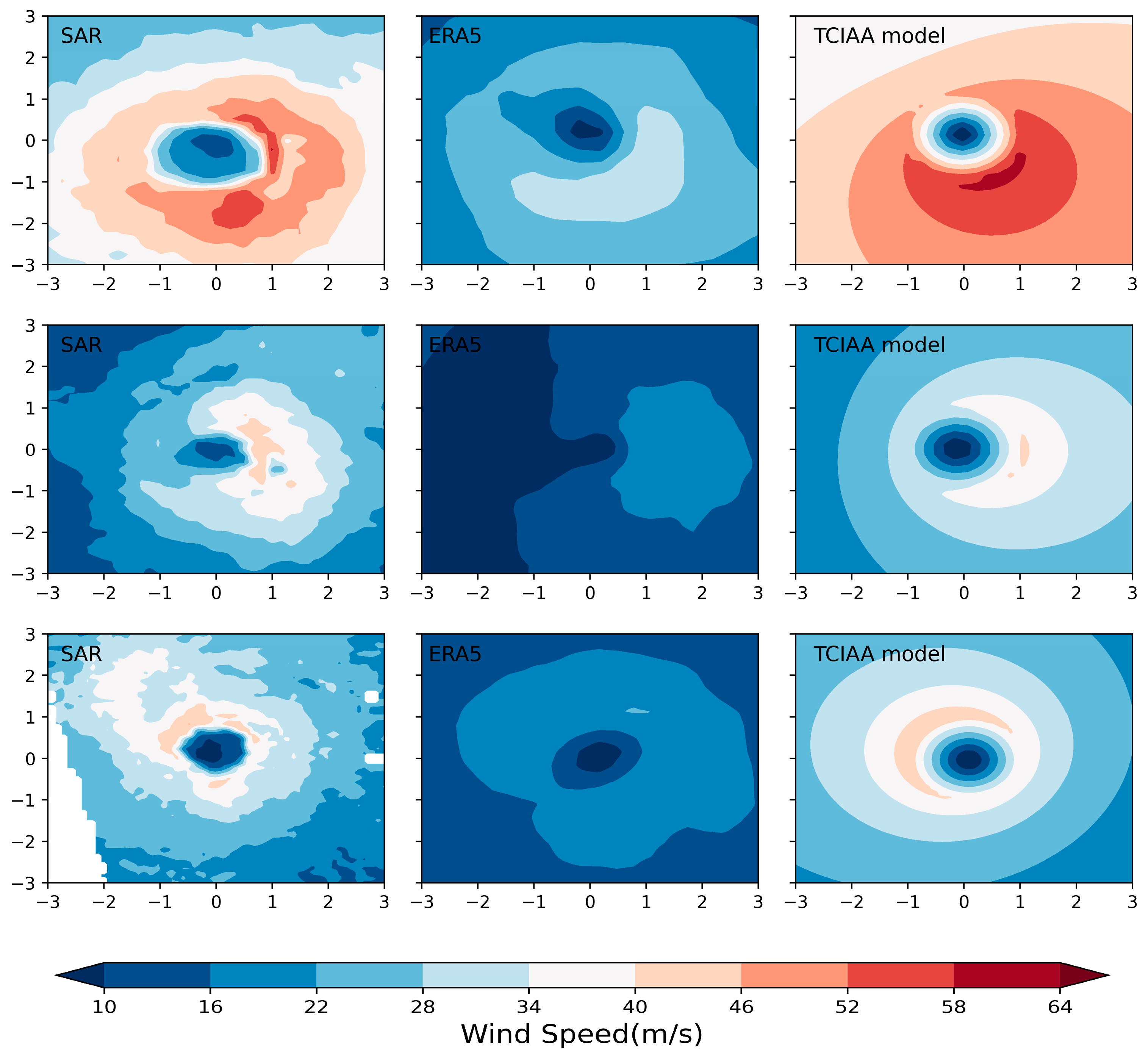
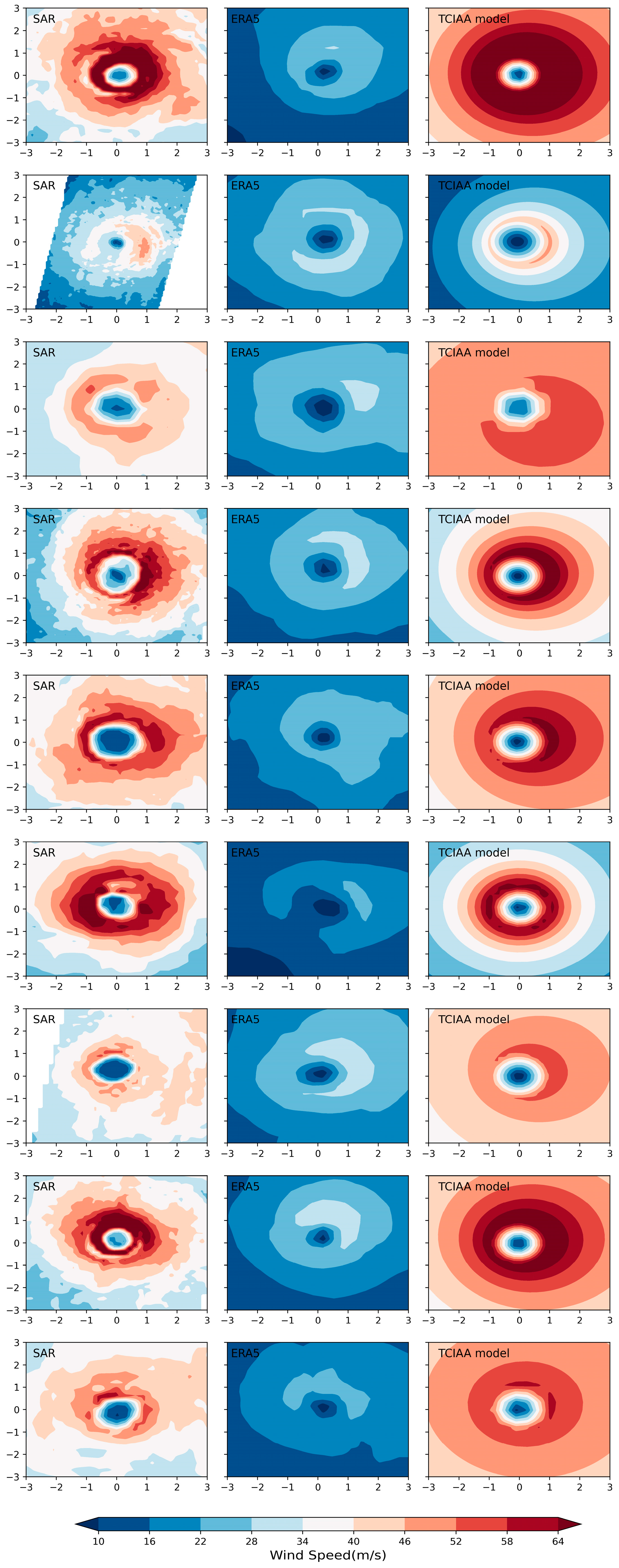
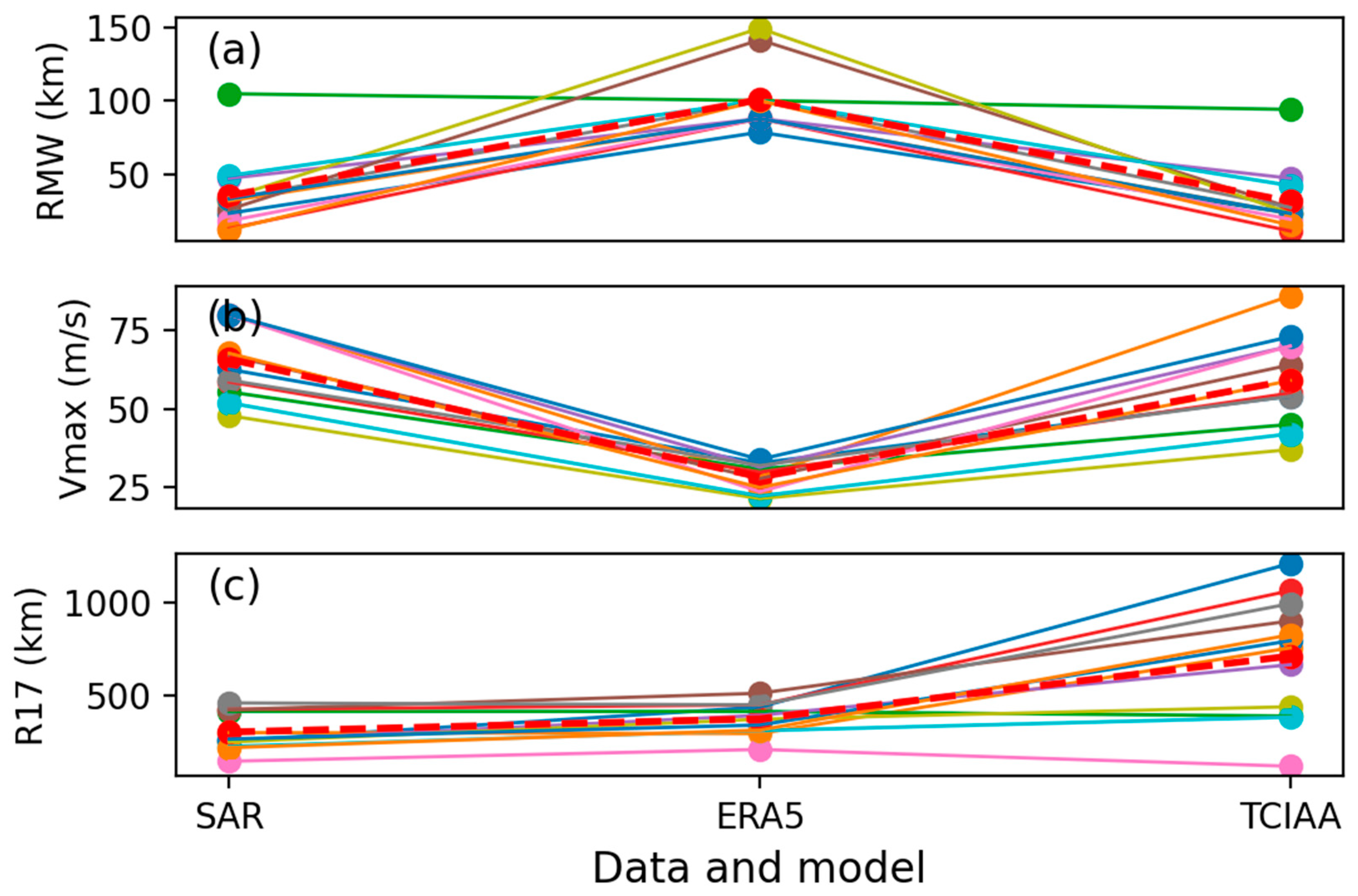
TCs are considered to be intense when they have a small inner-core (or small RMW) and higher maximum winds [36,37]. The TC size can also be represented by R17, which is the radius of the outermost circulation. There were several snapshots (belonging to 12 TCs) with missing values below 30%, and so we first chose one time from each TC as examples. To see the relationship between TC winds and SST, the above 12 times were further divided into two categories based on SST: one was located on the cooler sea surface (SST < 26.5 °C), and the other was located on the warmer (SST > 26.5 °C). The wind fields within 3 radii of the maximum wind (3RMW) from the SAR, ERA5, and TCIAA models over both colder and warmer surface water are shown in Figure 2 and Figure 3, respectively. The three physical parameters calculated from the different products are shown in Figure 4.
The 12 TC samples of SAR TC wind fields show the entire structure of the wind within 3RMW, with clearly visible TC eyes with calm winds (Figure 2 and Figure 3). The double eyewall in some TCs can also be seen in the higher resolution SAR data, but cannot be resolved in either of the other data products. Ten TCs have maximum wind speeds exceeding 50 m/s.
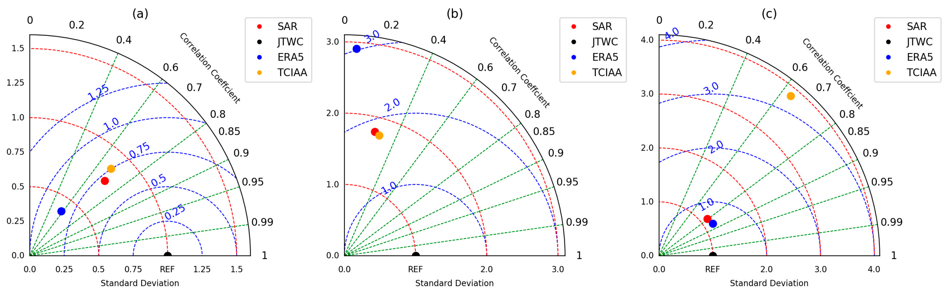
The JTWC data are taken as the reference, and we calculated the three parameters for all 44 TC times. The standard deviation of the maximum wind speed in SAR, ERA5, and TCIAA was 11.32, 5.8, and 12.69, with their average values of maximum wind being 56.71 m/s, 26.26 m/s, and 50.11 m/s, respectively. The corresponding correlation coefficients with the JTWC data were 0.71, 0.58, and 0.68, respectively. The normalized Taylor diagram of the maximum wind speed also demonstrated that SAR shows the best agreement, TCIAA shows the medium, and ERA5 shows the worst (Figure 5a).
We also compared the inner-core and the outermost circulation of the 44 TC snapshots to JTWC. The mean and standard deviation for RMW/R17, as well as the correlation coefficients with JTWC, were also presented in Table 1. The RMW and R17 of the normalized Taylor diagram showed that the ranking from the best to the worst was TCIAA, SAR, and ERA5 for RMW, while the ranking was ERA5, SAR, and TCIAA for R17 (Figure 5b,c). Based on the evaluation of the maximum wind speed and RMW together with R17, the comprehensive assessment demonstrated that SAR was the best overall product for describing the intensity and structure of TCs.
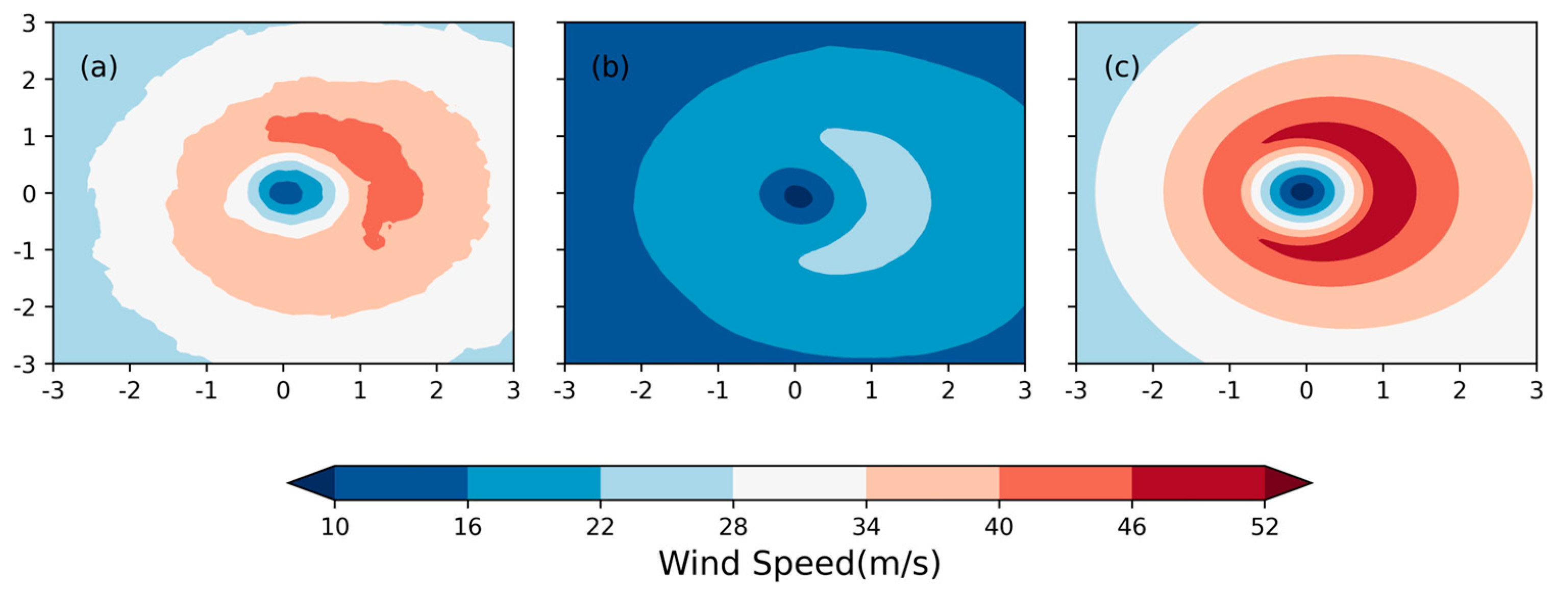
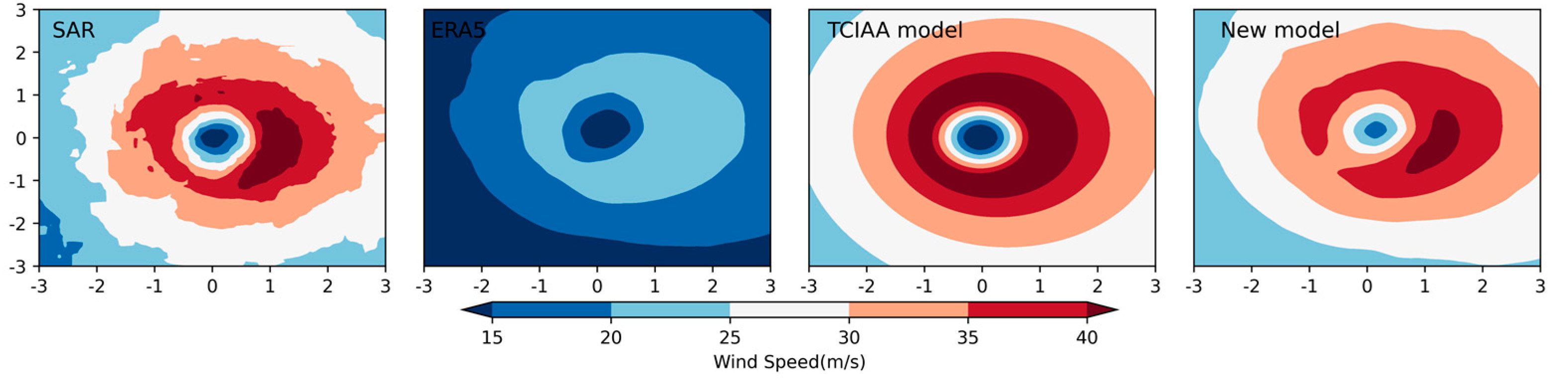
The above 44 TC times were all rotated into an along-track and cross-track coordinate system so that the TCs all moved along the y-axis. The resulting composite TC maps for the three products are shown in Figure 6. The spatial patterns for all data products were quite similar. However, while the TC magnitude in both SAR and TCIAA was similar, the TC magnitude in the ERA5 product was much smaller (which agreed with a previous study [38]). Note that the TCIAA model is based on SAR observational data and could be used to replenish missing values in SAR images.
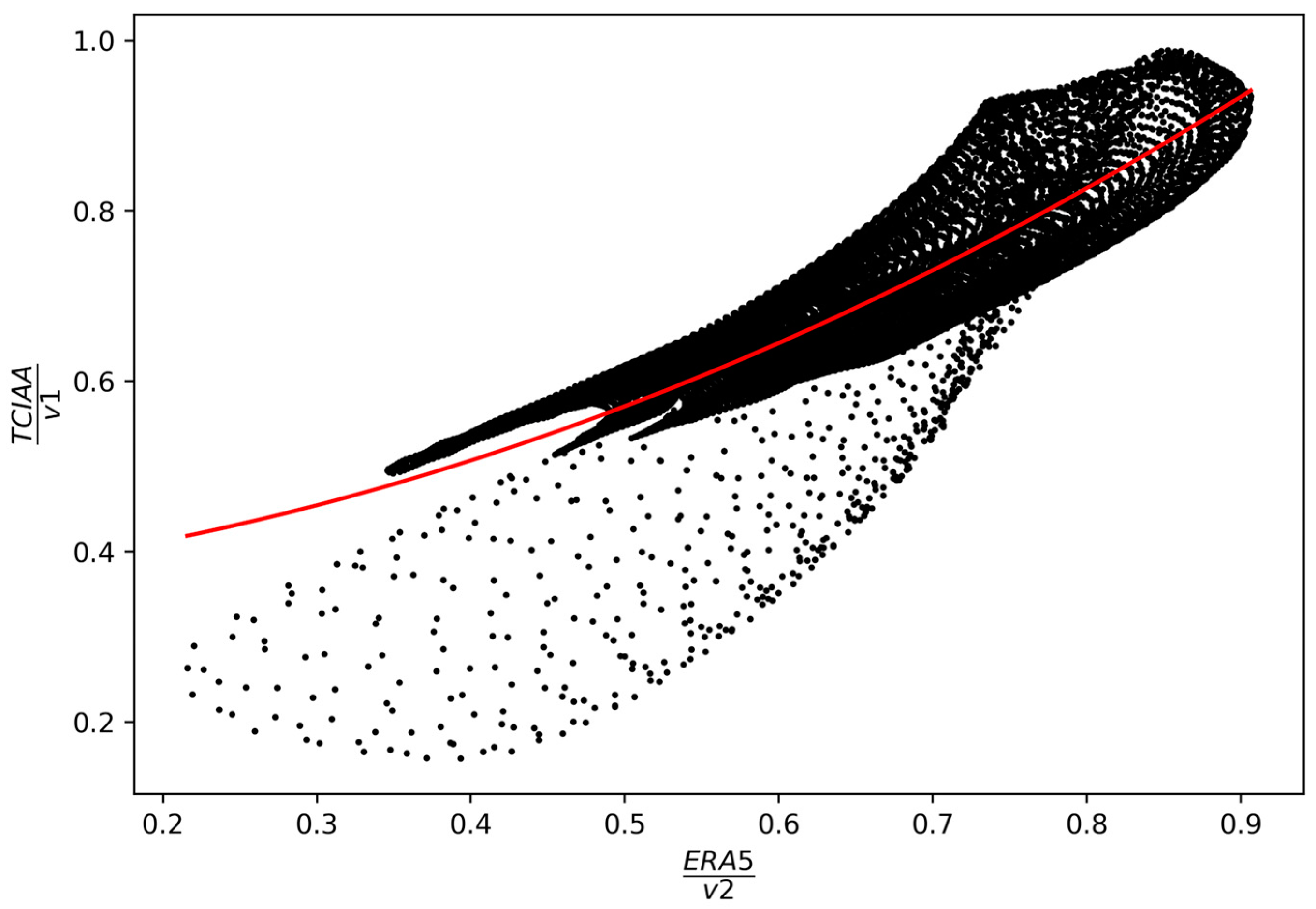
Considering that SAR data are not available for all TCs, while ERA5 data are, we further tried to construct a new TC model based on ERA5 data alone using the above assessment. We first randomly selected 30 times from the 44 TC times and constructed an empirical relationship between SAR observations and the other data products, including the TCIAA model and the reanalysis data mentioned above. We assumed the form of . Note that the first two model terms have been set to ensure that both the spatial pattern and the magnitude in the new wind product are similar to SAR. We derived a, b, and α when the correlation coefficient was the largest and the standard deviation was the smallest between the new data and the corresponding SAR observation. The derived model was , where v1 and v2 were the maximum wind speed in the TCIAA model and ERA5 data, respectively. The empirical relationship between the average coefficients and on each grid was computed and is presented in Figure 7. The scatter diagram shows a rough quadratic relationship, so a quadratic fitting was used to obtain the general relationship between these coefficients. As a result, the final new TC model for the ERA5 data product was where .
The remaining 14 TC times were used to assess the accuracy of the new ERA5 fitted model. It can be seen that the new model did a much better job describing the average TC wind field than the ERA5 data (Figure 8). In particular, both the spatial distribution and the location of maximum wind speed agreed well with the SAR wind field. The correlation coefficient between the new ERA5 model and the SAR was 0.92 (statistically significant at the 90% confidence level), suggesting that the new model using only ERA5 inputs can be used to reconstruct a reasonably accurate structure of the TC wind field.
3.2. The Influence of SST on TC Wind Field and Precipitation
When a TC passes over the sea surface, the high wind speed increases the evaporation rate and provides moisture that feeds the TC rainfall. In addition, strong vertical motions in the convective system of a TC can transport horizontal momentum downward to the low layers and increase the wind speed near the surface [39]. Consequently, the interaction between precipitation and the wind field is quite complex.
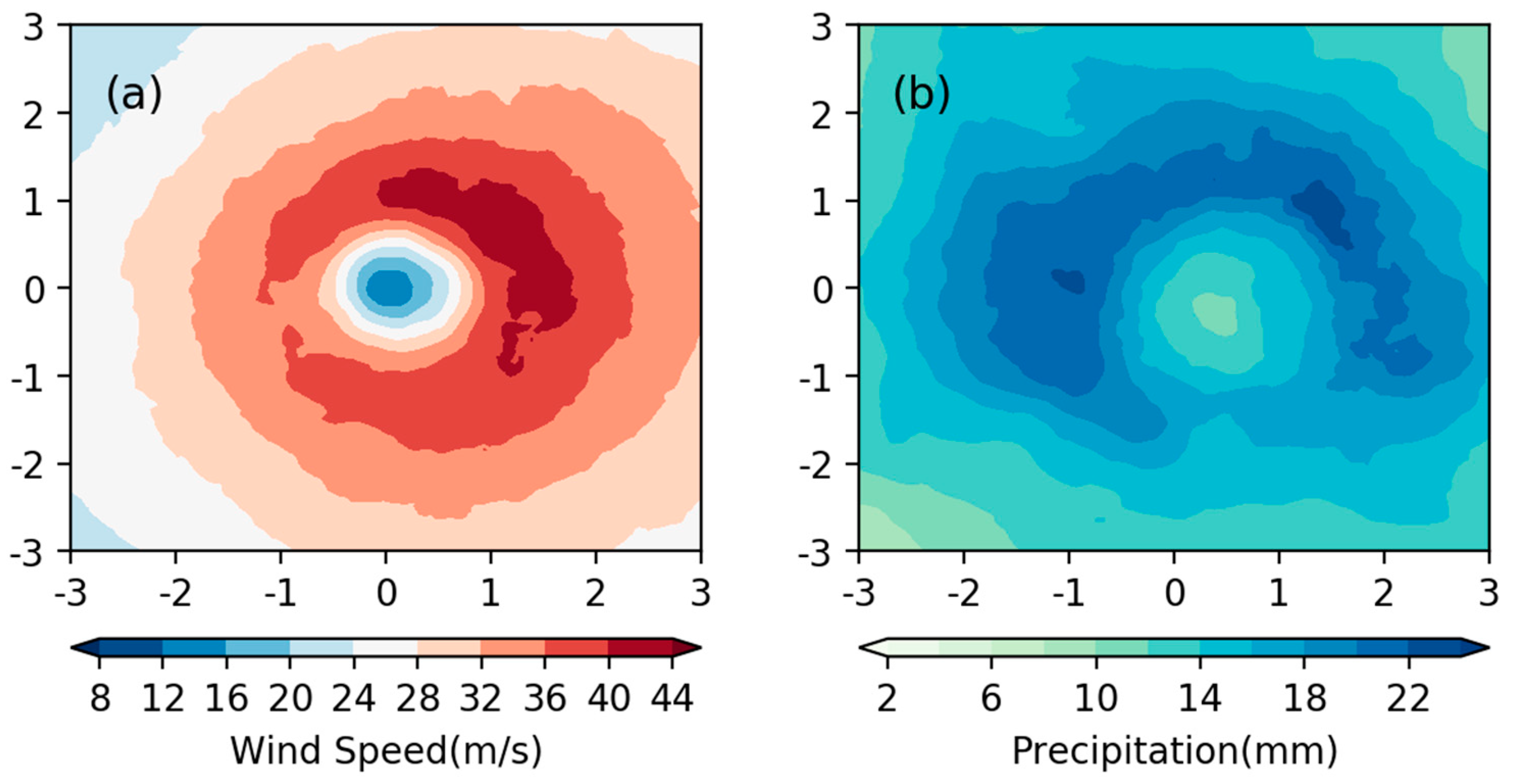
Figure 9 shows the average distributions of SAR wind speed and GPM precipitation for all 44 TC times. It was found that the larger precipitation value was located in the front right quadrant of the TC’s motion. The correlation coefficient between winds and precipitation was 0.669, which is significant at the 90% confidence level. This verifies that TC rainfall is larger when the TC wind speed is stronger.
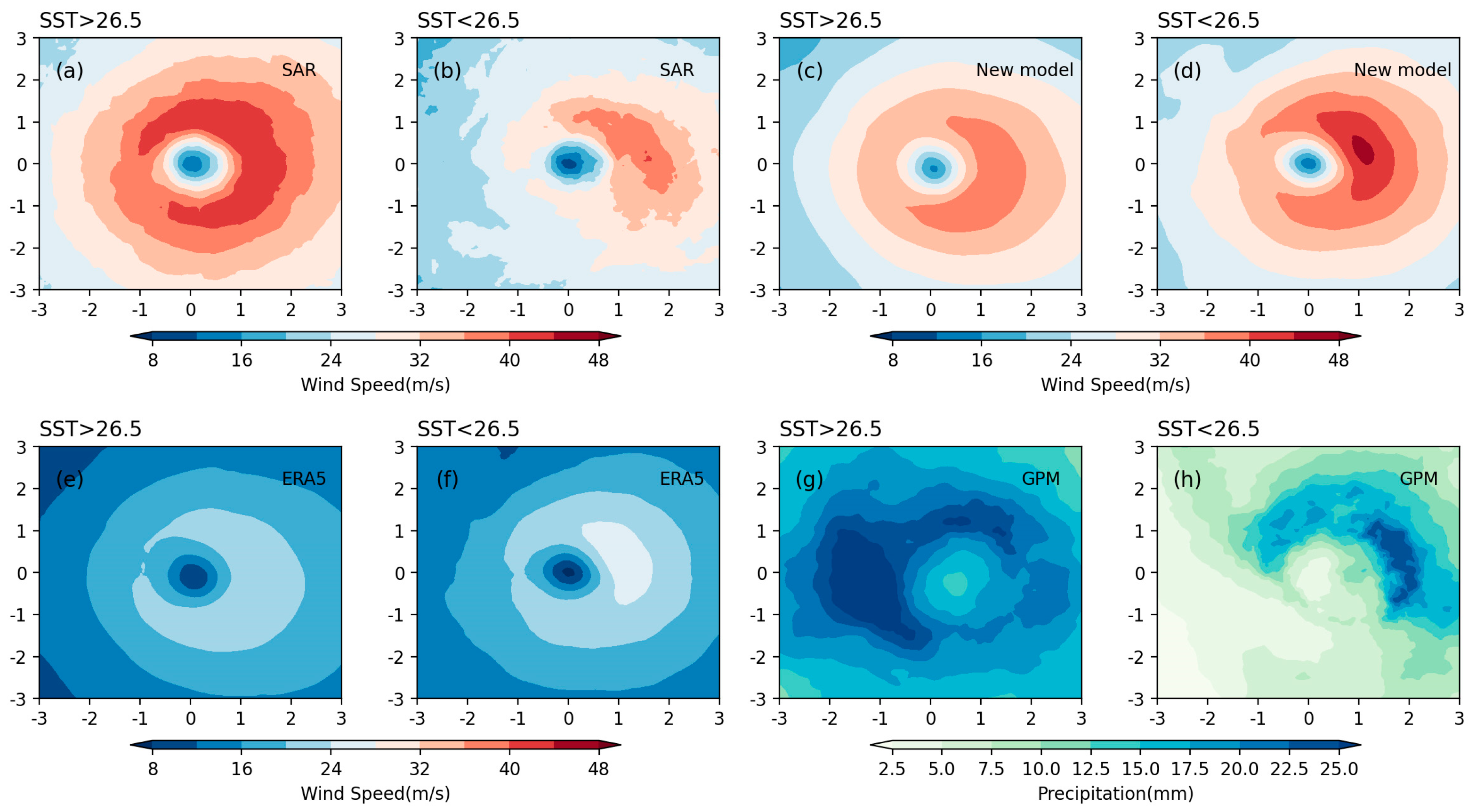
Generally, a warmer ocean enhances tropical cyclones and provides more rainfall. However, both tropical cyclone winds and rainfall can cool the sea surface by entrainment and heat flux exchange processes. How SST influences the correlation between TC winds and precipitation is not yet clear. Therefore, the 44 severe TC times were divided into two categories based on whether the underlying along-track SST was greater than or less than 26.5 °C. Overall, there were 11 TC times in which the underlying SST was lower than 26.5 °C and 33 times when it was higher than 26.5 °C. The distributions of the TC average surface wind field and precipitation are shown in Figure 10.
In the SAR data product, the maximum wind speed was located in the front right quadrant of the TC’s track (Figure 10a), independent of the SST. It is interesting to note that the TC’s intensity was weaker (stronger) when SST was cooler (warmer) than 26.5 °C (Figure 10a vs. Figure 10b). For TC rainfall, the most intense precipitation always appeared in the front left quadrant of the TC’s track when the sea surface was warmer, while the most intense precipitation was weaker and appeared to the right of the TC’s track when the sea surface was cooler (Figure 10g,h). The spatial correlation coefficient between precipitation and TC wind speed from SAR was 0.748 (0.649) when the SST was cooler (warmer) than 26.5 °C. This result suggests that the wind is a more important factor in influencing TC rainfall than SSR under cooler sea surface conditions. The results are similar when using the wind product from the new ERA5 fitted model. It is worth mentioning that the TC rainfall asymmetries can also be affected by vertical wind shear and storm motion [40,41]. Therefore, these factors need to be further investigated in the future.
4. Conclusions
The surface wind field data from high resolution synthetic aperture radar (SAR) with ERA5 reanalysis, and the TCIAA model simulation were used to analyze TC wind structures over the Western North Pacific between 2012 and 2020. Our results suggest that SAR data can accurately estimate the surface wind field structure and give good estimates of the maximum wind speed, RMW, and R17.
Based on the differences between ERA5 and SAR for TC winds, a new model for TC winds was developed to use ERA5 reanalysis data alone. Our results indicated that this new ERA5 fitted model could provide an accurate estimation of the TC wind field. This model was able to accurately reconstruct the TC wind structure for all TC snapshots, with improved wind speeds estimated compared to the ERA5 data. Limited by the quantity of severe TCs observed by SAR, as well as the missing values in SAR data, there might be some differences in some of the TC times. As a result, with new methods such as machine learning, as well as more observational data available in the future, the TC wind field model should also be further investigated and developed.
When a TC propagates over a warmer sea environment (SSTs higher than 26.5 °C), the wind field is stronger and the rainfall is more intense. There is also a strong positive correlation between wind speed and precipitation under TC conditions, with the correlation being higher under cooler sea surface conditions.
The relationship between wind and precipitation involves complicated dynamic and thermodynamic processes. In addition, the rain perturbations can result from changes in the sea surface roughness by impinging drops and can influence the wind vector retrieval [42]. As a result, their connection needs to be further explored. We expect that improving the knowledge of this relationship can be useful for reconstructing better TC wind fields in the future.
Author Contributions
Analyses of the data and preparation of the manuscript, R.D.; methodology, G.Z.; provided important insights, B.H. All authors have read and agreed to the published version of the manuscript.
Funding
This research was funded by the National Key Research and Development Program of China (2019YFC1510102).
Data Availability Statement
The SAR wind speed data come from Professor Zhang Biao from Nanjing University of Information Science and Technology, and the email is [email protected]; the TC dataset was downloaded from https://www.ncei.noaa.gov/products/international-best-track-archive (accessed on 28 September 2021) (noaa.gov). The precipitation dataset was downloaded from https://disc.gsfc.nasa.gov/datasets/GPM_3IMERGHH_06/summary (accessed on 15 December 2021). The ERA5 dataset was downloaded from https://cds.climate.copernicus.eu/cdsapp#!/dataset/reanalysis-era5-single-levels?tab=overview (accessed on 21 April 2022). The monthly SST dataset was downloaded from https://www.psl.noaa.gov/data/gridded/data.cobe.html (accessed on 27 April 2022).
Acknowledgments
I would like to express my thanks to all teachers who have helped me. First, a special acknowledgment should be shown to Zhang Biao, who provided the SAR wind speed dataset; the SAR data are the basis of my research. I would also like to express my thanks to my supervisor, Wang Guihua, who gave me important suggestions and kind encouragement as well as great help in the writing of this manuscript.
Conflicts of Interest
The authors declare no conflict of interest.
References
- Chen, L.; Xu, Y. Review of Typhoon Very Heavy Rainfall in China. Meteorol. Environ. Sci. 2017, 40, 3–10. [Google Scholar]
- Done, J.; Ge, M.; Holland, G.; Dima, I.; Phibbs, S.; Saville, G.; Wang, Y. Modelling global tropical cyclone wind footprints. Nat. Hazards Earth Syst. Sci. 2020, 20, 567–580. [Google Scholar] [CrossRef]
- Lu, Y.; Zhao, H.; Zhao, D.; Qingqing, L. Spatial-temporal characteristic of tropical cyclone disasters in China during 1984–2017. Haiyang Xuebao 2021, 43, 45–61. [Google Scholar]
- Emanuel, K.A. The dependence of hurricane intensity on climate. Nature 1987, 326, 483–485. [Google Scholar] [CrossRef]
- Knutson, T.R.; Tuleya, R.E. Impact of CO2-Induced Warming on Simulated Hurricane Intensity and Precipitation: Sensitivity to the Choice of Climate Model and Convective Parameterization. J. Clim. 2004, 17, 3477–3495. [Google Scholar] [CrossRef]
- Knutson, T.R.; McBride, J.L.; Chan, J.; Emanuel, K.; Holland, G.; Landsea, C.; Held, I.; Kossin, J.P.; Srivastava, A.K.; Sugi, M. Tropical cyclones and climate change. Nat. Geosci. 2010, 3, 157–163. [Google Scholar] [CrossRef]
- Webster, P.J.; Holland, G.J.; Curry, J.A.; Chang, H.-R. Changes in Tropical Cyclone Number, Duration, and Intensity in a Warming Environment. Science 2005, 309, 1844–1846. [Google Scholar] [CrossRef]
- Guishan, Y. Historical change and future trends of storm surge disaster in China’s coastal area. J. Nat. Disasters 2000, 9, 23–30. [Google Scholar]
- Emanuel, K.A. Increasing destructiveness of tropical cyclones over the past 30 years. Nature 2005, 436, 686–688. [Google Scholar] [CrossRef]
- Ge, Y.; Zhao, L.; Xiang, H. Review for numerical typhoon models based on extreme wind velocity prediction. J. Nat. Disasters 2003, 12, 31–40. [Google Scholar]
- Zhou, L.; Chen, D.; Lei, X.; Wang, W.; Wang, G.; Han, G. Progress and perspective on interactions between ocean and typhoon. Chin. Sci. Bull. 2019, 64, 60. [Google Scholar] [CrossRef]
- Ma, Y.; Zhang, Q. Approaches to Several Problems about Progress in the Study of Typhoon. J. Oceanogr. Huanghai Bohai Seas 1999, 17, 62–65. [Google Scholar]
- Russell, L.R. Probability Distributions for Hurricane Effects. J. Waterw. Harb. Coast. Eng. Div. 1971, 97, 139–154. [Google Scholar] [CrossRef]
- Batts, M.E.; Simiu, E.; Russell, L.R. Hurricane Wind Speeds in the United States. J. Struct. Div. 1980, 106, 2001–2016. [Google Scholar] [CrossRef]
- Holland, G.J. An Analytic Model of the Wind and Pressure Profiles in Hurricanes. Mon. Weather Rev. 1980, 108, 1212–1218. [Google Scholar] [CrossRef]
- Shapiro, L.J. The Asymmetric Boundary layer Flow Under a Translating Hurricane. J. Atmos. Sci. 1983, 40, 1984–1998. [Google Scholar] [CrossRef]
- Meng, Y.; Matsui, M.; Hibi, K. An analytical model for simulation of the wind field in a typhoon boundary layer. J. Wind Eng. Ind. Aerodyn. 1995, 56, 291–310. [Google Scholar] [CrossRef]
- Gao, Y.; Zhang, J.; Sun, J.; Guan, C. Application of SAR Data for Tropical Cyclone Intensity Parameters Retrieval and Symmetric Wind Field Model Development. Remote Sens. 2021, 13, 2902. [Google Scholar] [CrossRef]
- Zhang, G.; Li, X.; Perrie, W.; Zhang, J.A. Tropical Cyclone Winds and Inflow Angle Asymmetry From SAR Imagery. Geophys. Res. Lett. 2021, 48, e2021GL095699. [Google Scholar] [CrossRef]
- Fang, G.; Zhao, L.; Cao, S.; Ge, Y.; Pang, W. A novel analytical model for wind field simulation under typhoon boundary layer considering multi-field correlation and height-dependency. J. Wind Eng. Ind. Aerodyn. 2018, 175, 77–89. [Google Scholar] [CrossRef]
- Fang, G.; Zhao, L.; Cao, S.; Zhu, L.; Ge, Y. Estimation of tropical cyclone wind hazards in coastal regions of China. Nat. Hazards Earth Syst. Sci. 2020, 20, 1617–1637. [Google Scholar] [CrossRef]
- Snaiki, R.; Wu, T. A linear height-resolving wind field model for tropical cyclone boundary layer. J. Wind Eng. Ind. Aerodyn. 2017, 171, 248–260. [Google Scholar] [CrossRef]
- Jacob, S.D.; Koblinsky, C.J. Effects of Precipitation on the Upper-Ocean Response to a Hurricane. Mon. Weather Rev. 2007, 135, 2207–2225. [Google Scholar] [CrossRef]
- Jourdain, N.C.; Lengaigne, M.; Vialard, J.; Madec, G.; Menkes, C.E.; Vincent, E.M.; Jullien, S.; Barnier, B. Observation-Based Estimates of Surface Cooling Inhibition by Heavy Rainfall under Tropical Cyclones. J. Phys. Oceanogr. 2013, 43, 205–221. [Google Scholar] [CrossRef]
- Lin, Y.; Zhao, M.; Zhang, M. Tropical cyclone rainfall area controlled by relative sea surface temperature. Nat. Commun. 2015, 6, 6591. [Google Scholar] [CrossRef]
- Zhang, B.; Perrie, W. Cross-Polarized Synthetic Aperture Radar: A New Potential Measurement Technique for Hurricanes. Bull. Am. Meteorol. Soc. 2012, 93, 531–541. [Google Scholar] [CrossRef]
- Mouche, A.A.; Chapron, B.; Zhang, B.; Husson, R. Combined Co- and Cross-Polarized SAR Measurements Under Extreme Wind Conditions. IEEE Trans. Geosci. Remote Sens. 2017, 55, 6746–6755. [Google Scholar] [CrossRef]
- Sapp, J.W.; Alsweiss, S.O.; Jelenak, Z.; Chang, P.S.; Frasier, S.J.; Carswell, J.R. Airborne Co-polarization and Cross-Polarization Observations of the Ocean-Surface NRCS at C-Band. IEEE Trans. Geosci. Remote Sens. 2016, 54, 5975–5992. [Google Scholar] [CrossRef]
- Fernandez, D.E.; Carswell, J.R.; Frasier, S.; Chang, P.S.; Black, P.G.; Marks, F.D. Dual-polarized C- and Ku-band ocean backscatter response to hurricane-force winds. J. Geophys. Res. Ocean. 2006, 111, C08013. [Google Scholar] [CrossRef]
- Knapp, K.R.; Kruk, M.C.; Levinson, D.H.; Diamond, H.J.; Neumann, C.J. The International Best Track Archive for Climate Stewardship (IBTrACS): Unifying Tropical Cyclone Data. Bull. Am. Meteorol. Soc. 2010, 91, 363–376. [Google Scholar] [CrossRef]
- Kruk, M.C.; Knapp, K.R.; Levinson, D.H. A Technique for Combining Global Tropical Cyclone Best Track Data. J. Atmos. Ocean. Technol. 2010, 27, 680–692. [Google Scholar] [CrossRef]
- Levinson, D.; Diamond, H.; Knapp, K.; Kruk, M.; Gibney, E. Toward a Homogenous Global Tropical Cyclone Best-Track Dataset. Bull. Am. Meteorol. Soc. 2010, 91, 377–380. [Google Scholar]
- Jin, D.; Oreopoulos, L.; Lee, D.; Tan, J.; Cho, N. Cloud–Precipitation Hybrid Regimes and Their Projection onto IMERG Precipitation Data. J. Appl. Meteorol. Climatol. 2021, 60, 733–748. [Google Scholar] [CrossRef]
- Hersbach, H.; Bell, B.; Berrisford, P.; Hirahara, S.; Horányi, A.; Muñoz-Sabater, J.; Nicolas, J.; Peubey, C.; Radu, R.; Schepers, D.; et al. The ERA5 global reanalysis. Q. J. R. Meteorol. Soc. 2020, 146, 1999–2049. [Google Scholar] [CrossRef]
- Ishii, M.; Shouji, A.; Sugimoto, S.; Matsumoto, T. Objective analyses of sea-surface temperature and marine meteorological variables for the 20th century using ICOADS and the Kobe Collection. Int. J. Climatol. 2005, 25, 865–879. [Google Scholar] [CrossRef]
- Wu, L.; Tian, W.; Liu, Q.; Cao, J.; Knaff, J.A. Implications of the Observed Relationship between Tropical Cyclone Size and Intensity over the Western North Pacific. J. Clim. 2015, 28, 9501–9506. [Google Scholar] [CrossRef]
- Knaff, J.A.; Longmore, S.P.; DeMaria, R.T.; Molenar, D.A. Improved Tropical-Cyclone Flight-Level Wind Estimates Using Routine Infrared Satellite Reconnaissance. J. Appl. Meteorol. Climatol. 2015, 54, 463–478. [Google Scholar] [CrossRef]
- Hodges, K.; Cobb, A.; Vidale, P.L. How Well Are Tropical Cyclones Represented in Reanalysis Datasets? J. Clim. 2017, 30, 5243–5264. [Google Scholar] [CrossRef]
- Mechem, D.B.; Chen, S.S.; Houze, R.A., Jr. Momentum transport processes in the stratiform regions of mesoscale convective systems over the western Pacific warm pool. Q. J. R. Meteorol. Soc. 2006, 132, 709–736. [Google Scholar] [CrossRef]
- Rogers, R.; Chen, S.; Tenerelli, J.; Willoughby, H. A Numerical Study of the Impact of Vertical Shear on the Distribution of Rainfall in Hurricane Bonnie (1998). Mon. Weather Rev. 2003, 131, 1577–1599. [Google Scholar] [CrossRef]
- Chen, S.S.; Knaff, J.A.; Marks, F.D. Effects of Vertical Wind Shear and Storm Motion on Tropical Cyclone Rainfall Asymmetries Deduced from TRMM. Mon. Weather Rev. 2006, 134, 3190–3208. [Google Scholar] [CrossRef]
- Tournadre, J.; Quilfen, Y. Impact of rain cell on scatterometer data: 1. Theory and modeling. J. Geophys. Res. Ocean. 2003, 108, 3225. [Google Scholar] [CrossRef]
Figure 1.
The locations (dots) and the maximum wind speeds (dot color) of TCs observed by SAR and their tracks between 2012 and 2020. The solid black line shows the 2012 to 2020 climatological average 26.5 °C COBE sea surface temperature isotherm.
Figure 1.
The locations (dots) and the maximum wind speeds (dot color) of TCs observed by SAR and their tracks between 2012 and 2020. The solid black line shows the 2012 to 2020 climatological average 26.5 °C COBE sea surface temperature isotherm.

Figure 2.
The wind fields of 3 selected TC times in 3RMW, which were located on the cooler sea surface (SST < 26.5 °C): left column is from SAR data, middle column is from ERA5, and the right column is from the TCIAA model.
Figure 2.
The wind fields of 3 selected TC times in 3RMW, which were located on the cooler sea surface (SST < 26.5 °C): left column is from SAR data, middle column is from ERA5, and the right column is from the TCIAA model.

Figure 3.
Same as Figure 2, except for 9 TC times located on the warmer sea surface (SST > 26.5 °C).
Figure 3.
Same as Figure 2, except for 9 TC times located on the warmer sea surface (SST > 26.5 °C).

Figure 4.
The (a) RMW, (b) maximum wind speed, and (c) R17 for the 12 different TC times in Figure 2 and Figure 3 from the three data products: SAR, ERA5, and TCIAA models. The red dashed lines represent the average values.

Figure 5.
The normalized Taylor diagram of (a) the maximum wind speed, (b) RMW, and (c) R17 between SAR, ERA5, TCIAA, and JTWC data for all the 44 TC times.
Figure 5.
The normalized Taylor diagram of (a) the maximum wind speed, (b) RMW, and (c) R17 between SAR, ERA5, TCIAA, and JTWC data for all the 44 TC times.

Figure 6.
Average wind field distribution after rotation so that the y-axis is the TC translation direction for (a) SAR data, (b) ERA5, and (c) TCIAA models.
Figure 6.
Average wind field distribution after rotation so that the y-axis is the TC translation direction for (a) SAR data, (b) ERA5, and (c) TCIAA models.

Figure 7.
Scatter diagrams between average coefficient and average coefficient on each grid. The red solid curve is the quadratic fitting curve: y = 0.55x2 + 0.14x + 0.36, where y = and x = .
Figure 7.
Scatter diagrams between average coefficient and average coefficient on each grid. The red solid curve is the quadratic fitting curve: y = 0.55x2 + 0.14x + 0.36, where y = and x = .

Figure 8.
The average TC surface wind field structure for 14 TC times in SAR observation, ERA5, TCIAA model, and the ERA5 fitted model.
Figure 8.
The average TC surface wind field structure for 14 TC times in SAR observation, ERA5, TCIAA model, and the ERA5 fitted model.

Figure 9.
The distribution of (a) wind field from SAR and (b) precipitation from GPM. The storm has been rotated into along-track coordinates with the y-axis in the direction of TC translation.
Figure 9.
The distribution of (a) wind field from SAR and (b) precipitation from GPM. The storm has been rotated into along-track coordinates with the y-axis in the direction of TC translation.

Figure 10.
The along-track wind field distribution of (a) SAR, (c) the new model, (e) ERA5, and (g) the distribution of GPM precipitation when SST is higher than 26.5 °C; (b) SAR, (d) the new model, (f) ERA5, and (h) the distribution of precipitation when SST is lower than 26.5 °C.
Figure 10.
The along-track wind field distribution of (a) SAR, (c) the new model, (e) ERA5, and (g) the distribution of GPM precipitation when SST is higher than 26.5 °C; (b) SAR, (d) the new model, (f) ERA5, and (h) the distribution of precipitation when SST is lower than 26.5 °C.


Table 1.
The RMW, maximum wind speed and R17 statistics for all 44 different TCs in the following products: SAR, ERA5, and TCIAA models.
Table 1.
The RMW, maximum wind speed and R17 statistics for all 44 different TCs in the following products: SAR, ERA5, and TCIAA models.
| RMW | Vmax | R17 | |
|---|---|---|---|
| Mean | 47.37/116.1/44.64 | 56.71/26.26/50.11 | 273.96/357.77/557.46 |
| Standard deviation | 36.62/59.43/35.72 | 11.32/5.8/12.69 | 101.29/104.41/344.85 |
| Correlation with JTWC | 0.24/0.06/0.28 | 0.71/0.58/0.68 | 0.8/0.86/0.64 |
Disclaimer/Publisher’s Note: The statements, opinions and data contained in all publications are solely those of the individual author(s) and contributor(s) and not of MDPI and/or the editor(s). MDPI and/or the editor(s) disclaim responsibility for any injury to people or property resulting from any ideas, methods, instructions or products referred to in the content. |
© 2023 by the authors. Licensee MDPI, Basel, Switzerland. This article is an open access article distributed under the terms and conditions of the Creative Commons Attribution (CC BY) license (https://creativecommons.org/licenses/by/4.0/).
Share and Cite
MDPI and ACS Style
Du, R.; Zhang, G.; Huang, B. Observed Surface Wind Field Structure of Severe Tropical Cyclones and Associated Precipitation. Remote Sens. 2023, 15, 2808. https://doi.org/10.3390/rs15112808
AMA Style
Du R, Zhang G, Huang B. Observed Surface Wind Field Structure of Severe Tropical Cyclones and Associated Precipitation. Remote Sensing. 2023; 15(11):2808. https://doi.org/10.3390/rs15112808
Chicago/Turabian StyleDu, Rong, Guosheng Zhang, and Bin Huang. 2023. "Observed Surface Wind Field Structure of Severe Tropical Cyclones and Associated Precipitation" Remote Sensing 15, no. 11: 2808. https://doi.org/10.3390/rs15112808
Note that from the first issue of 2016, this journal uses article numbers instead of page numbers. See further details here.