
Generation of High Temporal Resolution Full-Coverage Aerosol Optical Depth Based on Remote Sensing and Reanalysis Data


1
College of Meteorology and Oceanography, National University of Defense Technology, Changsha 410037, China
2
School of Resources and Environment, University of Electronic Science and Technology of China, Chengdu 611731, China
*
Author to whom correspondence should be addressed.
Remote Sens. 2023, 15(11), 2769; https://doi.org/10.3390/rs15112769
Submission received: 8 April 2023
/
Revised: 21 May 2023
/
Accepted: 22 May 2023
/
Published: 26 May 2023
Abstract
:Aerosol Optical Depth (AOD) is a crucial physical parameter used to measure the radiative and scattering properties of the atmosphere. Obtaining full-coverage AOD measurements is essential for a thorough understanding of its impact on climate and air quality. However, satellite-based AOD products can be affected by abnormal weather conditions and high reflectance surfaces, leading to gaps in spatial coverage. To address this issue, we propose a satellite-based AOD filling method based on hourly level-3 Himawari-8 AOD products. In this study, the optimal model with a mean bias error (MBE) less than 0.01 and a root-mean-square error (RMSE) less than 0.1 in most land cover types was selected to generate the full-coverage AOD. The generated full-coverage AOD was validated against in situ measurements from the AERONET sites and compared with the performance of Himawari-8 AOD and MERRA-2 AOD over the AERONET sites. The validation results indicate that the accuracy of full-coverage AOD is comparable to that of the Advanced Himawari Imager (AHI) AOD, and for other land cover types (excluding barren land), the accuracy of full-coverage AOD is superior to that of MERRA-2 AOD. To investigate the practical application of full-coverage AOD, we utilized it as an input parameter to perform radiative transfer simulations in northwestern and southern China. The validation results showed that the simulated at-sensor radiance based on full-coverage AOD was in good agreement with the at-sensor radiance observations from MODIS. These results indicate that complete and accurate measurements of AOD have considerable potential for application in the simulation of at-sensor radiance and other related topics.
1. Introduction
Aerosols play a pivotal role in research related to the radiation balance, water cycle, and biogeochemical cycle owing to their relatively stable suspension system [1,2,3]. Aerosol Optical Depth (AOD) is one of the fundamental properties of aerosols, which characterizes the atmosphere’s ability to absorb and scatter radiation [4,5,6,7]. Additionally, the AOD serves as a crucial indicator of air pollution. Obtaining accurate and timely spatiotemporal AOD measurements is vital for monitoring the air pollution status and conducting research on climate change [8]. Ground observation, as an important method for obtaining high-precision AOD data, has the disadvantages of a small observation range, difficult setup, and high price, making it difficult to use for large-scale applications [9,10]. In contrast, satellite remote sensing has the advantages of continuous spatial coverage and rapid revisit cycles [11,12]. Consequently, satellite-based AOD has become an invaluable tool for monitoring air pollution on a large scale. However, its effectiveness can be limited by its sensitivity to various factors (e.g., abnormal weather conditions and high-reflectance surfaces), resulting in a considerable number of non-random gaps [13]. These gaps can restrict their application in certain research areas. Thus, obtaining full-coverage AOD products with gaps filled in has become a pressing concern [14].
Currently, many studies have established several full-coverage AOD models. Initially, a relatively simple statistical interpolation model is used to estimate the AOD at the missing pixels by analyzing the distribution of effective pixel values around the actual pixels of AOD [15,16,17,18,19]. Following previous work, some studies have tried to establish a regression model between AOD and input parameters (e.g., meteorological data and geospatial data) at the effective observation pixel of AOD and then apply the regression model to the missing region of AOD observation [20,21]. The development of machine learning methods has shown an increasingly strong ability for high-dimensional variable processing and nonlinear relationship fitting compared with traditional statistical interpolation models. Such an ability is conducive to establishing regression relationships between the AOD and multiple input parameters effectively [22,23,24]. On this basis, the introduction of AOD with high temporal resolution and spatially seamless estimates by the data assimilation model adds fresh insight to improve the accuracy of the satellite AOD retrieval algorithm [25,26].
In the past, geostationary meteorological satellites have been known to have a higher temporal resolution than polar-orbiting satellites. However, the spatial resolution of geostationary meteorological satellites was coarser, which created difficulties in accurately reflecting the changes in the spatial distribution of AOD. With the successful launch of Himawari-8 on 7 October 2014, the high-resolution AOD generated from the improved Advanced Himawari Imager (AHI) provided more opportunities for related studies [27]. The primary objective of this study is to build an AOD filling model based on Himawari-8 AOD products and to generate a full-coverage AOD product with high temporal resolution. At the same time, the full-coverage AOD was used as an input parameter to simulate the at-sensor radiance to evaluate the role of AOD products in the radiative transfer simulation.
2. Study Area and Datasets
2.1. Study Area
The selected study areas included the Northern Hemisphere (NH) within the Himawari-8 field of view and two sub-regions, including northwestern China (NC) and southern China (SC). The NH was used for producing full-coverage AOD products. The NC and SC sub-regions were selected to explore the applicability of the established full-coverage AOD products in the at-sensor radiance simulation with different environments because of their typical underlying surface.
The NH has a varied topography and a wide range of elevations. The land cover (LC) types in the region are diverse, including 17 LC types, such as forest, grassland, farmland, urban, and barren land [28]. The diverse LC types, complex terrain, and wide range of elevations provide a wide range of input parameters for the AOD filling algorithm, which is beneficial for broadening the application scenarios of the model. However, it also puts forward higher requirements for the AOD-filling algorithm in various usage scenarios. Figure 1 shows the LC-type map of the study areas and the distribution locations of the AERONET sites used in this study to validate the generated full-coverage AOD. More details of the sites can be found in Table A1.
The study area NC is in the Xinjiang Uygur Autonomous Region, with a longitude range of 81°E to 86°E and a latitude range of 38°N to 42°N. The climate is characterized by a temperate continental climate, while the underlying surface is primarily barren. The study area SC is located at the junctions of Guizhou Province, Guangxi Province, and Guangdong Province, with a longitude range of 108°E to 112°E and a latitude range of 22°N to 26°N. The climate is a subtropical monsoon climate, and the underlying surfaces are farmland and natural vegetation.
2.2. Datasets
2.2.1. Satellite Products
The satellite products used in this study included the AHI AOD product, the at-sensor radiance product (MOD02HKN), and the surface reflectance product (MOD09GA). AHI is onboard Himawari-8, which began operation in July 2015 and is in an equatorial synchronous orbit of approximately 35,800 km at 140.7°E [29]. It is capable of frequent and flexible observation, providing full-disk images of the earth every 10 min and regional images with shorter intervals. Full-disk and other regional observations have spatial resolutions of 0.5 to 2 km and spectral coverage incorporating 16 bands (3 for visible, 3 for near-infrared, and 10 for infrared). The AHI AOD retrieval algorithm selects the optimal channel for AOD retrieval by incorporating the weight of each AHI channel into the objective function. After that, different algorithms are employed to retrieve the AOD for land and ocean surfaces. Finally, the retrieval lookup table of AOD is established in the wavelength range of 300~2500 nm with a step of 1 nm to obtain AOD. In this study, the Level 3 AHI AOD with an hourly temporal resolution and a spatial resolution of 5 km × 5 km is used as the prediction target of the AOD filling algorithm in the study.
MOD02HKN, derived from the Moderate Resolution Imaging Spectroradiometer (MODIS), was used for the at-sensor observation simulation in this study. MODIS onboard the Terra/Aqua satellite was launched on 18 February 1999. MODIS consists of 36 medium-resolution spectral bands that are capable of observing land/cloud characteristics, ocean water color, surface temperature, and water vapor. The MOD02HKN radiance product is the channel radiance product of Terra MODIS. The spatial resolution of MOD02HKN is 250 m for bands 1–2 (0.62–0.672 μm, 0.841–0.89 μm), and 500 m for bands 3–7 (0.459–0.479 μm, 0.545–0.565 μm, 1.23–1.25 μm, 1.628–1.652 μm, 2.105–2.155 μm). Its original observation value is processed through radiance calibration and geographic correction. The visible band of MOD02HKN only provides daytime observations.
To validate the use of full-coverage AOD in at-sensor radiance simulation, a large-scale and high-precision surface reflectance product is needed. The MODIS surface reflectance product, MOD09GA, has eliminated the influence of atmospheric scattering and absorption and demonstrated high accuracy (with an error of less than 5%) [30]. Therefore, MOD09GA is used to provide a reliable surface background field for the radiative transfer simulation.
2.2.2. Reanalysis Datasets
The reanalysis datasets utilized in this study included the ERA5 reanalysis dataset and the MERRA-2 reanalysis dataset. The ERA5 reanalysis dataset was mainly used as the input parameters of the AOD filling algorithm. It was obtained from the European Centre for Medium-Range Weather Forecasts (ECMWF) and had a spatial resolution of 0.25° × 0.25° with an hourly temporal resolution [31]. The dataset used in this study included Total Cloud Cover (TCC), 2 m temperature (T2M), Surface Pressure (PS), 2 m u-component of wind (U2M), 2 m v-component of wind (V2M), Planetary Boundary Layer Height (PBLH), and Total Column Water Vapor (TCWV). The MERRA-2 reanalysis dataset was the latest version of the global atmospheric reanalysis dataset produced by NASA’s Global Simulation and Assimilation Office, using the Global Modeling and Assimilation Office (GMAO). The dataset covers land, sea, and atmospheric data products from 1980 to the present [32]. In this study, the TXTEXTTAU AOD of MERRA-2 M2T1NXAER with an hourly temporal resolution and a spatial resolution of 0.625° × 0.5° was used as an important input parameter of the AOD filling algorithm.
2.2.3. Auxiliary Data
The auxiliary data used in this study consisted of the 16-day normalized difference vegetation index (NDVI) product (MYD13C1), yearly LC type product (MCD12C1), Digital Elevation Model (DEM), Gridded Population of World Version 4 (GPWv4), and in situ data. MYD13C1 and MCD12C1 are the products of MODIS with a spatial resolution of 0.05° × 0.05°. MYD13C1 provided the NDVI product, which was computed from atmospherically corrected bi-directional surface reflectance masked for water, clouds, heavy aerosols, and cloud shadows [33]. MCD12C1 provided a global LC-type map with the IGBP classification scheme [28]. The Shuttle Radar Topography Mission (SRTM) DEM, with a resolution of 90 m, provided terrain relief information. GPWv4 provided population density information.
The in situ data from AERONET was used to evaluate the accuracy of full-coverage AOD with high temporal resolution. AERONET is a ground-based aerosol monitoring network by NASA and PHOtométrie pour le Traitement Opérationnel de Normalisation Satellitaire (PHOTONS), covering more than 500 sites worldwide. AERONET is equipped with a CIMEL CE318 sun and sky photometer with a detection band of 0.340 to 1.060 µm, and observations are made every 15 min or less [34]. A large number of studies have proven that AERONET AOD has a very high validation accuracy (±0.02) [35] and is often used as the “truth” to validate the accuracy of satellite-observed AOD. In this study, AERONET AOD (Level 2.0), which is cloud-filtered and quality validated [36], was selected for validation. The site’s information is shown in Table A1.
3. Methodology
3.1. Modelling Method
To generate the spatially seamless full-coverage AOD, the random forest (RF) algorithm was used to construct the nonlinear relationship between AHI AOD and various input parameters. The input parameters commonly used in the existing satellite AOD filling algorithm can be divided into four parts, including atmospheric parameters, surface parameters, socioeconomic parameters, and spatiotemporal parameters [37,38,39]. To ensure comprehensive data input, the selected input parameters included MERRA-2 AOD product (AODMERRA-2), atmospheric parameters (TCC, T2M, PS, U2M, V2M, and PBLH), observing geometric parameters including Solar Zenith Angle (SZA), Sensor Azimuth Angle (SAA), Solar Zenith Angle (SOZ), Solar Azimuth Angle (SOA), socioeconomic parameter (population density), and land surface parameters (NDVI, LC type, and DEM). Moreover, spatiotemporal parameters are also required in the AOD filling algorithm, including pixel geolocation, geographic distance from the pixel to the center, and four corners of the study area (Ucenter, Ubr, Ubl, Utr, Utl), local time (LT), and day-of-year (DOY).
To improve training accuracy, the total sample dataset was divided into various sample subsets. Since the LT and LC types are discrete variables that have an obvious influence on AHI AOD, the LT and LC types were used to divide the sample dataset. Based on the above considerations, we proposed three modeling methods, as follows:
- LC model: The total sample set was divided into 17 subsets according to the LC type, and the LC model was established for each subset as follows:where l (=1, 2, …, 16) represents the IGBP LC-type index.
- LT model: As the study areas are located in the northern hemisphere, sunlight hours were mainly concentrated between 8:00 and 17:00 LT, and AHI was only observed during daylight hours. Therefore, only observations from 8:00 to 17:00 LT were used as the data sample set for modeling. The data sample set was divided into 10 subsets according to LT, and the LT model was established for each subset as follows:where t (=8, 9, …, 17) represents LT.
- LT-LC model: Based on the analysis of the LC model and LT model, the total sample set was divided into 17 LC types and 10 LTs to obtain 170 subsets. The LT-LC model was established for each subset as follows:
3.2. Parameter Reselection and Combination
To avoid a decrease in model accuracy caused by antagonistic operation between input parameters, parameter reselection and a combination of the basic input parameters were performed. Moreover, this approach can also reduce the model training time and computational resources by minimizing the number of input parameters without compromising the model’s accuracy. Input parameters with strong linear correlations with retrieval targets were generally selected [6]. However, in the actual retrieval process, input parameters with a weak linear correlation can significantly improve the model’s accuracy. Therefore, we experimented with different combinations of input parameters and built separate full-coverage filling models using the same modeling approach. In detail, we compared the accuracy of the model’s test set for input parameter selection and evaluated the contribution of each input parameter to the model.
3.3. Validation Strategy
To ensure the credibility of in situ observations from AERONET stations and minimize the impact of random errors, spatiotemporal matching of AERONET in situ data, full-coverage AOD, and AHI AOD was performed. In the temporal dimension, the AERONET AOD was averaged over a time window set of ±30 min of the satellite scanning time. In the spatial dimension, the mean values of full-coverage AOD and AHI AOD, within a certain spatial distance centered around the AERONET site, were compared with in situ data. Generally, 5 × 5 or 3 × 3 spatial windows are preferred to calculate the spatial mean value [40]. In this study, a 3 × 3 spatial window was selected to calculate the spatial mean value to minimize the influence of topography and aerosol heterogeneity.
3.4. Satellite Observation Simulation
Forward radiative transfer simulation is essential in determining the dynamic range of the sensor, which helps ensure the reliability of sensor observations. Therefore, obtaining satellite observations beforehand and using them to assist in setting satellite sensor imaging parameters has become an important issue in optimizing satellite sensor designs [41,42]. At-sensor radiance simulation based on radiative transfer simulation is an effective method for addressing this problem. For radiative transfer simulation in the visible band, AOD plays an indispensable role. Therefore, the generated full-coverage AOD was introduced as the input parameter into an atmospheric radiative transfer simulation to simulate TOA radiance and compare the TOA radiance results with the MERRA-2 AOD as an input parameter and actual TOA observations to help validate the accuracy of the generated full-coverage AOD. This approach is also of great significance to satellite sensor simulation research [43]. Here, MODerate resolution atmospheric TRANsmission (MODTRAN), which has been widely used in academia, was used to simulate a broad range of high-precision visible bands [44,45].
To simulate the at-sensor radiance, one day for each season in NC and SC was selected. The simulation dates for NC were the 67th, 207th, 263rd, and 336th days of 2016. For SC, they were the 60th, 206th, 270th, and 334th days of 2016. The at-sensor radiance of MODIS channel 4, with full-coverage AOD and MERRA-2 AOD as AOD parameters, was simulated. Then, the two simulated at-sensor radiances were compared with the truth, i.e., the observed at-sensor radiance of MODIS channel 4. Moreover, the percentage of the radiance difference between the simulated and the observed was used as an indicator, which was calculated as follows:
where δm is the relative error between the simulated and the truth, expressed as a percentage; rsimulated and robserved are the simulated and observed at-sensor radiance, respectively.
3.5. Method Implementation
The input data for the experiments were taken from 2016, which were divided into different subsets according to the three different modeling schemes. The number of subsets for the three modeling methods (LC, LT, LC-LT) was 10, 17, and 170, respectively. Subsequently, the optimal structural parameters of the RF were determined using the grid search method. To balance the model training time and accuracy, 75% of the samples for each subset were utilized for training, while the remaining 25% were used for testing.
Once the model was constructed, the basic parameter combination was used as the input to establish the model. The optimal input parameter combination was selected, which provided the best performance for the model. Therefore, the corresponding model was called the optimal model. After determining the optimal model, we analyzed its performance at different LC types and different LTs. Subsequently, the generated full-coverage AOD was validated against the in situ AOD. Finally, the full-coverage AOD was taken as the input parameter for conducting simulation experiments and analyzing the accuracy of the results, which is of great significance to research on satellite sensor simulation. The flow chart of this study is shown in Figure 2.
4. Results
4.1. Model Results
Three RF models based on Equations (1–3) were established to obtain full-coverage AOD. The root-mean-square error (RMSE) and the percentage of samples within the expected error (EE) of the models at different LTs and LC types are shown in Figure 3. Figure 3a,b shows that the model accuracy of the three modeling methods varied with LT. Figure 3c,d shows that the model accuracy of the three modeling methods varied with the LC type. Among them, the LC model had the lowest model accuracy within almost different LTs and LC types, with an RMSE of 0.13–0.30 and an EE of about 60% within different LTs and an RMSE of 0.20–0.80 and an EE of 2% to 90% within different LC types. The accuracy of the LT model was the highest, with RMSE ranging from 0.03 to 0.14 and EE over 90% within different LTs and RMSE ranging from 0.05 to 0.28 and EE over 75% within different LC types.
By analyzing Figure 3a–d, two conclusions were made: (1) the LC model had the lowest model accuracy, and the two maximum RMSEs were found over mixed forest and ice and snow. Despite having a much larger number of training data compared with the LT-LC model, the LC model’s accuracy was lower, indicating that only using LC as an input parameter was insufficient to discriminate the differences between different land types. Instead, it was necessary to build a model for different LTs separately. (2) The LT-LC model training set was based on the LT model training set for different LC-type divisions of the results. However, the model accuracy of the LT-LC model was not improved based on the LT model. This shows that the improvement in model accuracy caused by changing the current modeling method was not enough to offset the negative effect of reducing the number of training samples on model accuracy. This suggests that modeling for different LC types is not necessary. Ultimately, the LT model was chosen as the optimal method for building the AOD filling model.
4.2. Parameter Combination Analysis
Figure 4 shows the RMSE of the model training set with different parameter combinations at different LC types, and the parameter combination codes of different input parameter combinations are shown in Table 1. It highlights that arbitrarily adding atmospheric parameters, sensor observation parameters, geolocation, and geographical distances as input parameters significantly improved the accuracy of the model. Land surface parameters, other than ice and snow, were added separately, which reduced the model’s accuracy. However, the presence of land surface parameters, together with the observed geometry, greatly improved the model’s accuracy. Population density did not improve model accuracy apart from input parameters. Interestingly, even without using MERRA-2 AOD as an input parameter, higher accuracy was achieved using a large number of remaining input parameters with weak linear correlations. The AHI AOD prediction model corresponding to C15 had the highest accuracy and therefore was used to predict the hourly full-coverage AOD in the study area in 2016.
4.3. Optimal Model Performance
According to the above, the LT model was the optimal modeling method, and C15 was the optimal parameter combination. The performance of the optimal model based on the optimal modeling method and the optimal parameter combination was studied. Figure 5 shows the MBE, RMSE, R, and EE of the optimal model based on the LT model, with C15 as the input parameter at different LT and LC types of modeling. The optimal model was referred to as the model for the convenience of description. The model had inconspicuous systematic deviations (MBE values are all less than 0.01) and had extremely high accuracy (RMSE values are all less than 0.1), except for waterbodies, stagnant shrubs, ice and snow, and barren land. For all LC types, the RMSE values of the model showed an obvious variation cycle with LT, i.e., the RMSE of the model was higher at 08:00 LT, then gradually decreased, reached a minimum around 10:00 LT, and then started to increase again, peaking at 13:00–14:00 LT, then gradually declined. The variation in RMSE at dissimilar LTs was mainly affected by the accuracy of AHI AOD at different LTs. In addition, there was a high correlation between the predicted results and the truth (R was greater than 0.9), and more than 80% of the predicted results were distributed within the EE range. The stagnant shrubs accounted for only 0.26% of the study area. The effective sample points obtained were 3230, which only accounted for 0.01% of the total sample number, far lower than the sample number of other LC types, resulting in the model being hard to fully train. For waterbodies, ice and snow, and barren land, previous studies revealed that AHI AOD performed the worst over sparsely vegetated surfaces but improved with the increase of NDVI values [46].
Figure 6 shows that most of the predicted value points on barren land were distributed in the EE interval and had a high correlation with the truth. However, there were some abnormal overestimation points in the low value range of the AHI AOD and some abnormal underestimation points in the high value range of the AHI AOD (as shown by the purple circle in Figure 6). To further investigate the causes of outlier points, the isolation forest was used to calculate the outlier degree of each sample point, and barren land was the research object [47]. The top 5% of the sample points of the outlier degree were regarded as outliers, and the remaining 95% were regarded as non-outliers. By comparing the distribution of the input parameters of outliers and non-outliers, the causes of abnormal prediction results were explored. Due to the validation results at 14:00 LT showing the poor performance of the validation accuracy, samples for barren land at 14:00 LT were separated from the outliers for further analysis of the causes. More details about the input parameter distributions of non-outliers and outliers isolated at 14:00 LT on barren land are shown in Figure 6k and Figure 7.
Figure 7 shows that there is an indistinct difference between outliers and non-outliers in the distribution of longitude, latitude, DEM, U2M, V2M, T2M, PS, and other parameters. Although the latitude distribution had a large difference in image appearance, the main reason for this is that the non-outlier values contained some of the lower latitude points, and the values from Figure 7 show that there is no significant difference in the latitude distribution. However, in terms of the AHI AOD distribution, outliers and non-outliers in barren areas showed obvious differences; the AHI AOD of non-outliers was generally small, mainly distributed between 0 and 0.5. The AHI AOD of outliers showed a large number of abnormally high values, mainly distributed between 1 and 3. In summary, the model of the main causes of low precision on barren land was that the AHI AOD of some of the sample points (5~8%) was abnormal. The relationship between outliers and input parameters had an obvious difference from the relationship between non-outliers and input parameters, making the model forecast a significant deviation in these points, which reduced the accuracy of the model.
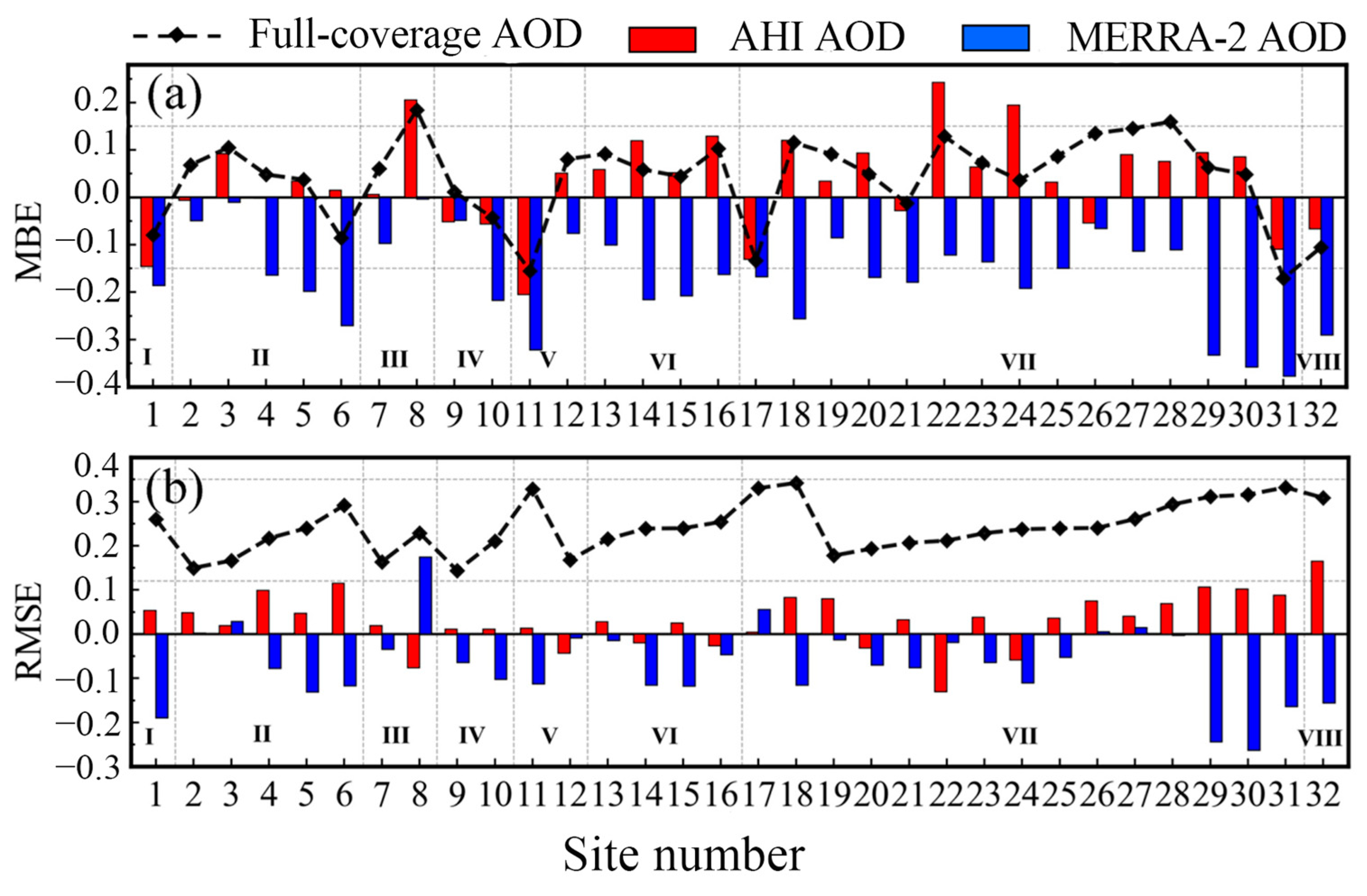
4.4. Site Validation
The full-coverage AOD filled by the LT model was validated against in situ AOD from AERONET data, and the selected AERONET stations are shown in Table A1. Figure 8a,b shows the MBE and RMSE results of full-coverage AOD, AHI AOD, and MERRA-2 AOD against in situ observations at 32 selected AERONET sites. According to Figure 8a, except for some urban sites (No. 21 and No. 23) and barren land sites (No. 32), the MBE of full-coverage AOD was less than 0.15, which was similar to the MBE of AHI AOD. The MBE of MERRA-2 AOD at all sites was less than 0, indicating that there was a significant systematic underestimation of MERRA-2 AOD. Figure 8b shows that the RMSE of full-coverage AOD was lower than 0.35 at all sites of LC types and lower than that of MERRA-2 at most sites. In conclusion, from the perspective of validation, the full-coverage AOD was similar to the AHI AOD with high accuracy. The accuracy was better than that of MERRA-2 AOD in most LC types. Figure 9 shows the scatterplot between the full-coverage AOD, MERRA-2 AOD, and AHI AOD and in situ AOD at No. 32, which had some abnormally high AHI AOD values. Similar outliers also occurred in the full-coverage AOD, with AHI AOD as the training target, which resulted in a reduction in validation accuracy. This also proved that the main reason for the low accuracy of the model on barren land was that there were some outliers in the AHI AOD.
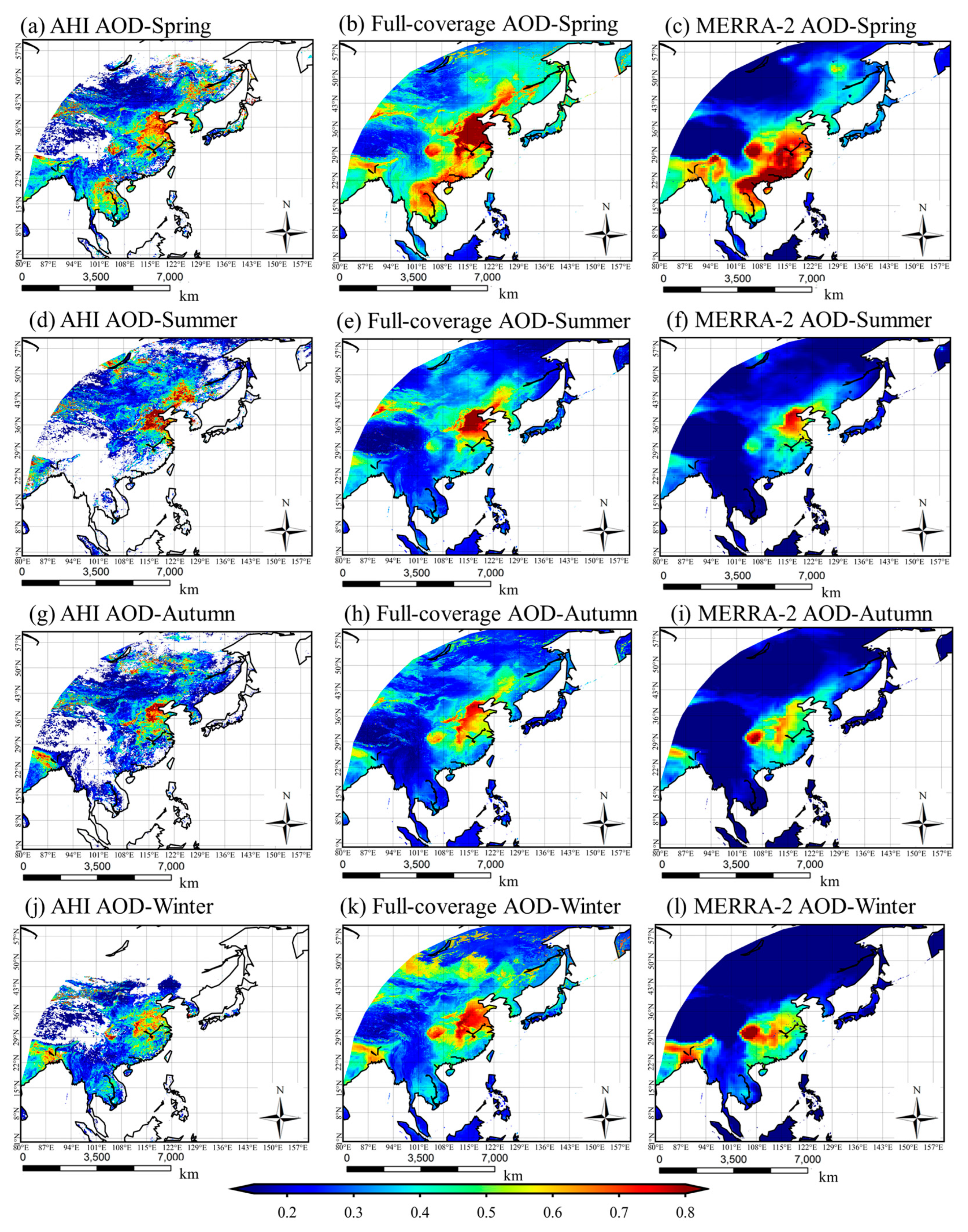
4.5. Spatiotemporal Distribution Analysis of Full-Coverage AOD
Based on the established optimal model, we generated the full-coverage AOD in the study area and analyzed its spatiotemporal distribution. Figure 10 shows the seasonal mean AOD of AHI, full-coverage, and MERRA-2 in spring (months 3–5), summer (months 6–8), autumn (months 9–11), and winter (months 12–2) within the study area, where (a,d,g,j) are AHI AOD, (b,e,h,k) are full-coverage AOD, and (c,f,i,l) is MERRA-2 AOD. As shown in Figure 10, AHI AOD had a low proportion of pixel-valid values (clear-sky AOD) in any season and had clear spatiotemporal variation characteristics. In spring, the proportion of the valid values in the whole study area was relatively high, and pixels with a proportion of 0 valid values only existed in the Qinghai Tibet Plateau and the northernmost part of the study area. In the grassland in the middle of the study area and the farmland vegetation in the south and northwest of the study area, the proportion of valid values of pixels was manifestly higher than that of other areas. In summer, the pixel area with valid values accounting for 0 gradually expanded, reaching a maximum in the southern study area. In autumn, the proportion of valid values in the southern and northwestern study areas further decreased, and the proportion of valid values in the southern study area reached its maximum. In winter, the proportion of valid values in the northern study area decreased significantly, and a large number of pixels with a valid value proportion of 0 appeared. However, the proportion of valid values in the southern study area increased. The main reason was the winter snow in the north, resulting in a reduction in the success rate of the AOD filling algorithm. In the southern region, the climate was dry in winter, which decreased the influence of clouds and fog on AOD retrieval, and the retrieval success probability of the AHI AOD algorithm increased.
The full-coverage AOD had a high spatiotemporal similarity with AHI AOD but had a significant difference from MERRA-2 AOD. Parts with higher AHI AOD and full-coverage AOD values were found in areas of population concentration or industrial density, e.g., northeastern China, eastern China, southern China, northeastern India, and Vietnam. In the grassland areas of northern and northeastern China, the mean AOD decreased but could still clearly reflect rich spatial details. Compared with AHI AOD, the mean value of MERRA-2 AOD was lower. The high-value region of the MERRA-2 AOD had a certain spatial dislocation compared with the AHI AOD, which was mainly concentrated in southeast China and south Asia. In the north and northwest of the study area, it was difficult to show the spatial distribution of AOD on barren land and grassland in the northern and northwestern study areas. Compared with AHI AOD, the mean value of full-coverage AOD significantly increased. One of the reasons for the absence of AHI AOD was the interference of clouds and fog. Moreover, the AOD in the area affected by clouds and fog was generally higher than that in non-cloud-affected areas, which is consistent with [25,48].
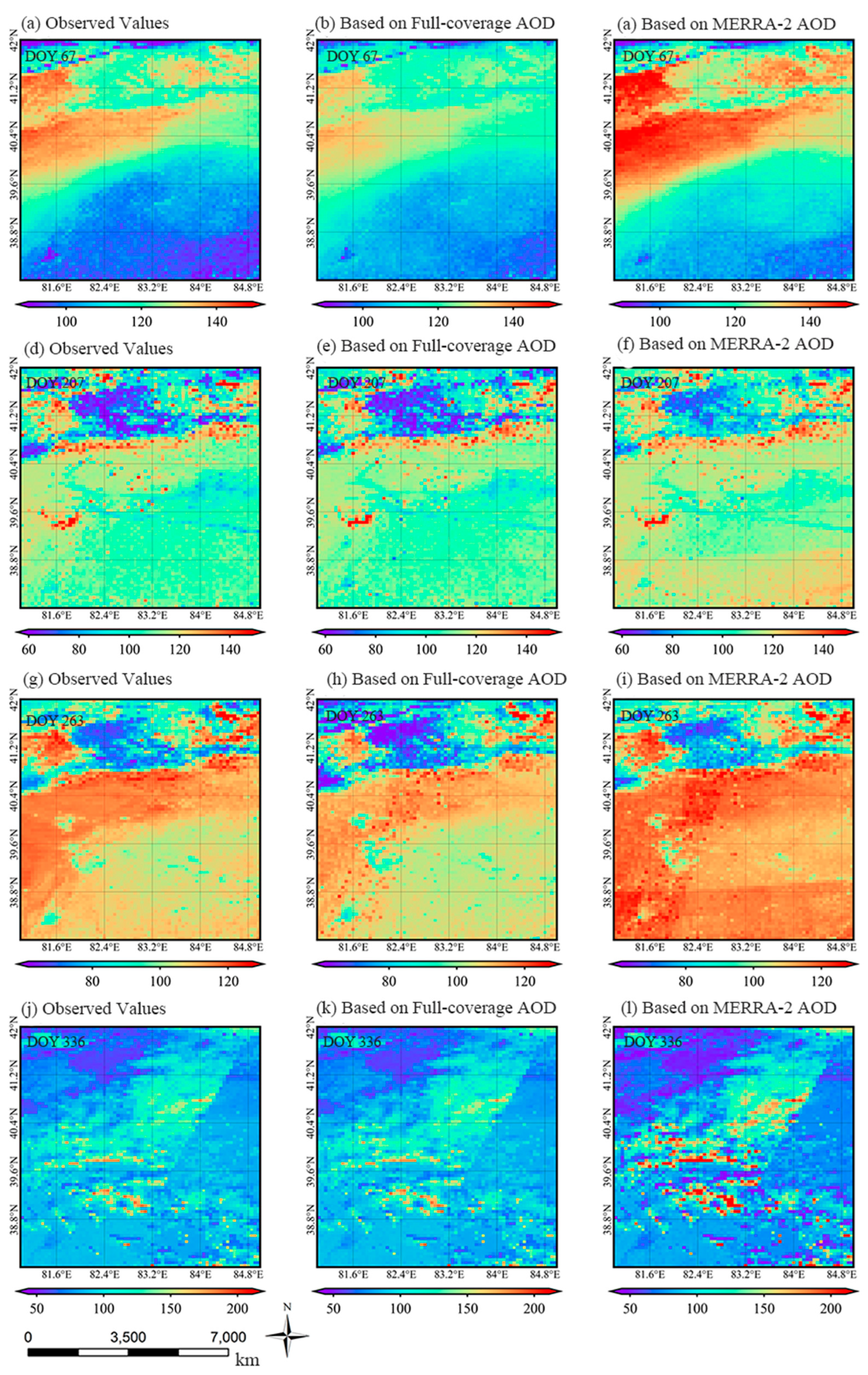
4.6. At-Sensor Radiance Simulation Results
To investigate the performance of full-coverage AOD, it was taken as the input parameter in the at-sensor radiance simulation. Table 2 shows the mean AOD of the full-coverage AOD and MERRA-2 AOD on selected days in NC and SC. The average AOD in SC was notably higher than that in NC. Moreover, the AOD values in both regions showed a certain seasonal cycle pattern, and the seasonal variation of the MERRA-2 AOD was larger than that of the full-coverage AOD. This could be related to the atmospheric water vapor difference between NC and SC.
Table 3 summarizes the statistical parameters of at-sensor radiance differences between the simulated and the truth on the 67th, 207th, 263rd, and 336th of 2016 for NC and the 60th, 206th, 270th, and 334th of 2016 for SC. Figure 11 shows the at-sensor radiance observed by MODIS Channel 4, and the simulation based on full-coverage AOD and MERRA-2 AOD on the corresponding dates in NC. Table 3 shows that the full-coverage AOD-based at-sensor radiance had a higher consistency with the truth in NC. In the four seasons, δm within ±5% between the truth and full-coverage AOD-based at-sensor radiance was 73.4–86.1%. A certain degree of systematic underestimation was found in spring (the proportion of pixels with the δm range of −20% to −5%). The MERRA-2 AOD-based at-sensor radiance showed significant overestimation in the four seasons. From the statistical results, it can be seen that the proportion of pixels with the δm in the range of 5% to 20% between the truth and the MERRA-2 AOD-based at-sensor radiance were higher than 20%. This was much larger than the corresponding value of the results based on the full-coverage AOD. The reason for the large difference between the simulation results obtained based on full-coverage AOD and the truth in spring was that clouds and fog appear more frequently in spring (approximately 50% of the pixels were obscured by clouds and fog). It reduced the accuracy of the full-coverage AOD in spring, resulting in the accuracy of the simulation results based on the full-coverage AOD. Nevertheless, even in areas affected by cloud cover, the precision of the simulation results based on the full-coverage AOD was still better than that based on the MERRA-2 AOD. The difference from the truth was less than an order of magnitude, which satisfied the sensor dynamics in practical applications. In addition, the underlying surface of NC was mainly desert, and the spatial distribution difference of AOD was inconspicuous. Therefore, there was no patch effect in the simulated image.
Figure 12 shows the at-sensor radiance observed by MODIS Channel 4, and simulated based on full-coverage AOD and MERRA-2 AOD on the selected dates in SC. Similar to the comparison in NC, the full-coverage AOD-based at-sensor radiance showed higher consistency with the truth in SC. In the four seasons, the proportion of pixels with δm within ±5% between the truth and the full-coverage AOD-based at-sensor radiance was 78.7–89.7%. The MERRA-2 AOD-based at-sensor radiance showed obvious underestimations in spring and autumn. In spring and autumn, the proportion of pixels with δm in the range of −20% to 5% between the truth and the MERRA-2 AOD-based at-sensor radiance was 68.2% and 38.3%, respectively. This is much higher than the corresponding value of the full-coverage AOD-based result. According to Table 3, the main reason for the underestimation was that the MERRA-2 AOD in SC was significantly higher in spring and autumn. The patch effect can also be found in the MERRA-2 AOD-based at-sensor radiance in Figure 12. The reason for the patch effect was that the MERRA-2 AOD in those sub-regions was significantly different from their adjacent regions. Meanwhile, the spatial resolution of the MERRA-2 AOD was much larger than the rest of the simulation input parameters. Therefore, the scale difference finally appeared as patches in the simulated image. Compared to NC, the underlying surface in SC was more heterogeneous. That is, the heterogeneity within the MERRA-2 AOD pixel led to a significant patch effect in the MERRA-2 AOD-based at-sensor radiance.
5. Discussion
To investigate and optimize the method for filling in the missing values of AOD, three different AOD filling methods based on the RF model were investigated based on selecting relevant input parameters. The key idea was to establish a relationship between the AOD and the relevant parameters. When compared with previous studies, such as introducing a data assimilation algorithm to generate full-coverage AOD [25], the approach in this study was straightforward and convenient. To explore full-coverage AOD in greater detail, future research could focus more on the introduction of weakly correlated factors and advanced deep-learning methods.
To evaluate the generated full-coverage AOD, it was compared with the in situ AOD from AERONET sites. Additionally, the simulated at-sensor radiance was also simulated based on the generated full-coverage AOD and MERRA-2 AOD. The findings suggest that the generated full-coverage AOD performed better than the MERRA-2 AOD, indicating that the method has the potential for producing full-coverage AOD. However, there are challenges with applying this method to nighttime full-coverage AOD, primarily due to a lack of mature nighttime AOD products and ground-based observations for validation.
6. Conclusions
To explore the influence of different RF model construction schemes and parameter selection on the accuracy of the AOD filling model to improve the accuracy of full-coverage AOD, the application effects of three different RF modeling methods in AOD filling were tested in this study. The results of accuracy statistics showed that the LT model had the highest model accuracy, with an RMSE of 0.04–0.13. The full-coverage AOD was validated based on the in situ data of AERONET sites, and the RMSE of the validation results was 0.14–0.34. In addition, the spatial distribution variations of the four seasonal average AHI AOD, full-coverage AOD, and MERRA-2 AOD were analyzed so that the spatial distribution of full-coverage AOD was more consistent with AHI AOD and contained more spatial details than that of MERRA-2 AOD.
We took the full-coverage AOD as the input parameter and used MODTRAN to conduct simulation experiments in northwestern China and southern China to analyze the accuracy of the simulation results. The results showed that the simulation results based on the full-coverage AOD had high consistency with the truth in northwestern China and southern China. However, the simulation results based on the MERRA-2 AOD showed overestimation in northwestern China and underestimation in the spring and autumn of southern China. In conclusion, the accuracy and image quality of at-sensor simulation results based on full-coverage AOD compared with the truth in the simulation were promoted, meeting the design objective of providing suggestions for setting the dynamic range of sensors in practical applications. The AOD filling model proposed in this study has positive research significance in the field of satellite at-sensor simulation.
Aiming at the problem of AOD filling, we established an optimal model from the two perspectives of modeling selection and parameter combination to obtain a full-coverage AOD. In addition, atmospheric radiative transfer simulation was based on full-coverage AOD to validate its applicability. However, due to the lack of existing nighttime AOD products with high accuracy as the label value, nighttime AOD research has not been carried out, and the exploration of night AOD retrieval and filling can be studied in the future.
Author Contributions
Conceptualization, Z.L. and J.M.; methodology, Z.L. and Z.J.; software, validation, formal analysis, investigation; resources, Z.J. and Y.M.; data curation, J.M.; writing—original draft preparation, Z.L.; writing—review and editing, Y.M. and J.M.; visualization, Y.M.; supervision, J.M. and Z.L. All authors have read and agreed to the published version of the manuscript.
Funding
This research was funded by the project “Research on Meteorological Support Application of Satellite Data”.
Data Availability Statement
Data available on request from the authors.
Acknowledgments
The authors would like to thank the Japan Aerospace Exploration Agency (JAXA) (https://global.jaxa.jp/, (accessed on 7 April 2023)) for providing AHI AOD and the Copernicus Climate Change Service (C3S) (https://cds.climate.copernicus.eu/, (accessed on 7 April 2023)) for providing the ERA5 data. We also thank EARTH DATA for providing MODIS (https://earthdata.nasa.gov, (accessed on 7 April 2023)), GPWv4 for providing population density data (https://sedac.ciesin.columbia.edu, (accessed on 7 April 2023)), the Goddard Space Flight Center (GSFC) for providing AERONET (https://aeronet.gsfc.nasa.gov, (accessed on 7 April 2023)), and the Geospatial Data Cloud site, Computer Network Information Center, Chinese Academy of Sciences, for providing DEM (http://www.gscloud.cn/, (accessed on 7 April 2023)).
Conflicts of Interest
The authors declare no conflict of interest.
Appendix A

Table A1.
AERONET sites information.
| Site Name | Number | Longitude | Latitude | LC Type |
|---|---|---|---|---|
| Luang_Namtha | 1 | 20.9311 | 101.4162 | 2 |
| Ussuriysk | 2 | 43.7004 | 132.1635 | 4 |
| KORUS_Daegwallyeong | 3 | 37.68712 | 128.7587 | 4 |
| Hankuk_UFS | 4 | 37.33883 | 127.2658 | 4 |
| KORUS_Taehwa | 5 | 37.31248 | 127.3103 | 4 |
| DRAGON_Hankuk_UFS | 6 | 37.33883 | 127.2658 | 4 |
| KORUS_UNIST_Ulsan | 7 | 35.5819 | 129.1897 | 8 |
| Omkoi | 8 | 17.79833 | 98.43167 | 9 |
| Silpakorn_Univ | 9 | 13.81931 | 100.0412 | 9 |
| Chiang_Mai_Met_Sta | 10 | 18.77113 | 98.97247 | 9 |
| Gangneung_WNU | 11 | 37.771 | 128.867 | 12 |
| KORUS_Mokpo_NU | 12 | 34.91342 | 126.4374 | 12 |
| KORUS_Songchon | 13 | 37.33849 | 127.4895 | 12 |
| KORUS_Baeksa | 14 | 37.41156 | 127.5691 | 12 |
| KORUS_Iksan | 15 | 35.9622 | 127.0052 | 12 |
| Gandhi_College | 16 | 25.871 | 84.12794 | 12 |
| XiangHe | 17 | 39.7536 | 116.9615 | 12 |
| Pusan_NU | 18 | 35.23535 | 129.0825 | 13 |
| KORUS_Kyungpook_NU | 19 | 35.88999 | 128.6064 | 13 |
| Ubon_Ratchathani | 20 | 15.24552 | 104.871 | 13 |
| DRAGON_NIER | 21 | 37.56893 | 126.6397 | 13 |
| Seoul_SNU | 22 | 37.45806 | 126.9511 | 13 |
| KORUS_Olympic_Park | 23 | 37.52165 | 127.1242 | 13 |
| Yonsei_University | 24 | 37.56443 | 126.9348 | 13 |
| EPA-NCU | 25 | 24.96753 | 121.1855 | 13 |
| KORUS_NIER | 26 | 37.56893 | 126.6397 | 13 |
| Chen-Kung_Univ | 27 | 22.99342 | 120.2047 | 13 |
| Beijing-CAMS | 28 | 39.93333 | 116.3167 | 13 |
| Beijing | 29 | 39.97689 | 116.3814 | 13 |
| NGHIA_DO | 30 | 21.04778 | 105.7996 | 13 |
| Chiayi | 31 | 23.49598 | 120.496 | 14 |
| Dalanzadgad | 32 | 43.57722 | 104.4192 | 16 |
References
- Dubovik, O.; Holben, B.N.; Eck, T.F.; Smirnov, A.; Slutsker, I. Variability of Absorption and Optical Properties of Key Aerosol Types Observed in Worldwide Locations. J. Atmos. 2002, 59, 590–608. [Google Scholar] [CrossRef]
- Huang, R.-J.; Zhang, Y.; Bozzetti, C.; Ho, K.-F.; Cao, J.-J.; Han, Y.; Daellenbach, K.R.; Slowik, J.G.; Platt, S.M.; Canonaco, F.; et al. High secondary aerosol contribution to particulate pollution during haze events in China. Nature 2014, 514, 218–222. [Google Scholar] [CrossRef] [PubMed]
- Levy, H.; Horowitz, L.W.; Schwarzkopf, M.D.; Ming, Y.; Golaz, J.-C.; Naik, V.; Ramaswamy, V. The roles of aerosol direct and indirect effects in past and future climate change. J. Geophys. Res. Atmos. 2013, 118, 4521–4532. [Google Scholar] [CrossRef]
- Hänel, G. The Properties of Atmospheric Aerosol Particles as Functions of the Relative Humidity at Thermodynamic Equilibrium with the Surrounding Moist Air. Adv. Geophys. 1976, 19, 73–188. [Google Scholar] [CrossRef]
- Semenov, V.K.; Smirnov, A.; Aref’ev, V.N.; Sinyakov, V.P.; Sorokina, L.I.; Ignatova, N.I. Aerosol optical depth over the mountainous region in central Asia (Issyk-Kul Lake, Kyrgyzstan). Geophys. Res. Lett. 2005, 32, L05807. [Google Scholar] [CrossRef]
- Wang, D.; Zhang, F.; Yang, S.; Xia, N.; Ariken, M. Exploring the spatial-temporal characteristics of the aerosol optical depth (AOD) in Central Asia based on the moderate resolution imaging spectroradiometer (MODIS). Environ. Monit. Assess. 2020, 192, 383. [Google Scholar] [CrossRef]
- Zipfel, L.; Andersen, H.; Cermak, J. Machine-Learning Based Analysis of Liquid Water Path Adjustments to Aerosol Perturbations in Marine Boundary Layer Clouds Using Satellite Observations. Atmosphere 2022, 13, 586. [Google Scholar] [CrossRef]
- Mao, J.T.; Zhang, J.H.; Wang, M.H. Summary comment on research of atmospheric aerosol in China. J. Meteorol. Res. 2002, 60, 625–634. [Google Scholar] [CrossRef]
- Chubarova, N.Y.; Poliukhov, A.A.; Gorlova, I.D. Long-term variability of aerosol optical thickness in Eastern Europe over 2001–2014 according to the measurements at the Moscow MSU MO AERONET site with additional cloud and NO2 correction. Atmos. Meas. Tech. 2016, 9, 313–334. [Google Scholar] [CrossRef]
- Sherman, J.P.; Sheridan, P.J.; Ogren, J.A.; Andrews, E.; Hageman, D.; Schmeisser, L.; Jefferson, A.; Sharma, S. A multi-year study of lower tropospheric aerosol variability and systematic relationships from four North American regions. Atmos. Chem. Phys. 2015, 15, 12487–12517. [Google Scholar] [CrossRef]
- Alexandrov, M.D.; Geogdzhayev, I.V.; Tsigaridis, K.; Marshak, A.; Cairns, B. New statistical model for variability of aerosol optical thickness: Theory and application to MODIS data over ocean. J. Atmos. Sci. 2015, 73, 151201150243008. [Google Scholar] [CrossRef] [PubMed]
- Barnaba, F.; Gobbi, G.P. Aerosol seasonal variability over the Mediterranean region and relative impact of maritime, continental and Saharan dust particles over the basin from MODIS data in the year 2001. Atmos. Chem. Phys. 2004, 4, 188. [Google Scholar] [CrossRef]
- Zhao, C.; Liu, Z.; Wang, Q.; Ban, J.; Chen, N.X.; Li, T. High-resolution daily AOD estimated to full coverage using the random forest model approach in the Beijing-Tianjin-Hebei region. Atmos. Environ. 2019, 203, 70–78. [Google Scholar] [CrossRef]
- Engel-Cox, J.A.; Holloman, C.H.; Coutant, B.W.; Hoff, R.M. Qualitative and quantitative evaluation of MODIS satellite sensor data for regional and urban scale air quality. Atmos. Environ. 2004, 38, 2495–2509. [Google Scholar] [CrossRef]
- Leptoukh, G.; Zubko, V.; Gopalan, A. Spatial aspects of multi-sensor data fusion: Aerosol optical thickness. In Proceedings of the International Geoscience and Remote Sensing Symposium, Barcelona, Spain, 23–27 July 2007. [Google Scholar] [CrossRef]
- Lv, B.; Hu, Y.; Chang, H.H.; Russell, A.G.; Bai, Y. Improving the Accuracy of Daily PM2.5 Distributions Derived from the Fusion of Ground-level Measurements with Aerosol Optical Depth Observations, a Case Study in North China. Environ. Sci. Technol. 2016, 50, 4752. [Google Scholar] [CrossRef]
- Nirala, M. Multi-sensor data fusion of aerosol optical thickness. Int. J. Remote Sens. 2008, 29, 2127–2136. [Google Scholar] [CrossRef]
- Yang, J.; Hu, M. Filling the missing data gaps of daily MODIS AOD using spatiotemporal interpolation. Sci. Total Environ. 2018, 633, 677–683. [Google Scholar] [CrossRef]
- Zhou, C.Y.; Liu, Q.H.; Tang, Y.; Wang, K.; Sun, L. Comparison between MODIS aerosol product C004 and C005 and evaluation of their applicability in the north of China. J. Remote Sens. 2009, 13, 854–872. [Google Scholar] [CrossRef]
- Gao, L.; Jun, L.I.; Chen, L.; Zhang, L. Retrieval Atmospheric Aerosol Optical Depth over China from AVHRR by Multiple Regression Method. J. Atmos. Environ. Opt. 2015, 10. [Google Scholar] [CrossRef]
- Li, G.; Chen, W.; Li, R.; Chen, Y.; Li, L. Prediction of AOD data by geographical and temporal weighted regression with nonlinear principal component analysis. Arab. J. Geosci. 2020, 13. [Google Scholar] [CrossRef]
- Di, Q.; Kloog, I.; Koutrakis, P.; Lyapustin, A.; Wang, Y.; Schwartz, J. Assessing PM2.5 Exposures with High Spatiotemporal Resolution across the Continental United States. Environ. Sci. Technol. 2016, 50, 4712–4721. [Google Scholar] [CrossRef] [PubMed]
- Pu, Q.; Yoo, E.H. Ground PM2.5 prediction using imputed MAIAC AOD with uncertainty quantification. Environ. Pollut. 2021, 274, 116574. [Google Scholar] [CrossRef] [PubMed]
- Tang, D.; Liu, D.; Tang, Y.; Seyler, B.C.; Zhan, Y. Comparison of GOCI and Himawari-8 aerosol optical depth for deriving full-coverage hourly PM2.5 across the Yangtze River Delta. Atmos. Environ. 2019, 217, 116973. [Google Scholar] [CrossRef]
- Jiang, T.; Chen, B.; Nie, Z.; Ren, Z.; Tang, S. Estimation of hourly full-coverage PM2.5 concentrations at 1-km resolution in China using a two-stage random forest model. Atmos. Res. 2020, 248, 105146. [Google Scholar] [CrossRef]
- Xiao, Q.; Wang, Y.; Chang, H.H.; Xia, M.; Yang, L. Full-coverage high-resolution daily PM 2.5 estimation using MAIAC AOD in the Yangtze River Delta of China. Remote Sens. Environ. 2017, 199, 437–446. [Google Scholar] [CrossRef]
- Yoshida, M.; Kikuchi, M.; Nagao, T.M.; Murakami, H.; Nomaki, T.; Higurashi, A. Common Retrieval of Aerosol Properties for Imaging Satellite Sensors. J. Meteorol. Soc. Jpn. Ser. II 2018, 96, 193–209. [Google Scholar] [CrossRef]
- Friedl, M.; Sulla-Menashe, D. MCD12Q1 MODIS/Terra+Aqua Land Cover Type Yearly L3 Global 500m SIN Grid. NASA EOSDIS Land Process. DAAC 2019, 10, 200. [Google Scholar] [CrossRef]
- Bessho, K.; Date, K.; Hayashi, M.; Ikeda, A.; Imai, T.; Inoue, H.; Kumagai, Y.; Miyakawa, T.; Murata, H.; Ohno, T.; et al. An Introduction to Himawari-8/9—Japan’s New-Generation Geostationary Meteorological Satellites. J. Meteorol. Soc. Jpn. Ser. II 2016, 94, 151–183. [Google Scholar] [CrossRef]
- Liang, S.; Fang, H.; Chen, M.; Shuey, C.J.; Walthall, C.; Daughtry, C.; Morisette, J.; Schaaf, C.; Strahler, A. Validating MODIS land surface reflectance and albedo products: Methods and preliminary results. Remote Sens. Environ. 2002, 83, 149–162. [Google Scholar] [CrossRef]
- Hersbach, H.; Bell, B.; Berrisford, P.; Hirahara, S.; Horányi, A.; Muñoz-Sabater, J.; Nicolas, J.; Peubey, C.; Radu, R.; Schepers, D.; et al. The ERA5 global reanalysis. Q. J. R. Meteorol. Soc. 2020, 146, 1999–2049. [Google Scholar] [CrossRef]
- Rienecker, M.M.; Suarez, M.J.; Gelaro, R.; Todling, R.; Bacmeister, J.; Liu, E.; Bosilovich, M.G.; Schubert, S.D.; Takacs, L.; Kim, G.-K.; et al. MERRA: NASA’s Modern-Era Retrospective Analysis for Research and Applications. J. Clim. 2011, 24, 3624–3648. [Google Scholar] [CrossRef]
- Didan, K.; Huete, A. MYD13C1 MODIS/Aqua Vegetation Indices 16-Day L3 Global 0.05Deg CMG. NASA EOSDIS Land Process. DAAC 2015. Available online: https://lpdaac.usgs.gov/products/myd13c1v006/ (accessed on 7 April 2023).
- Kahn, R.A.; Gaitley, B.J.; Garay, M.J.; Diner, D.J.; Eck, T.F.; Smirnov, A.; Holben, B.N. Multiangle Imaging SpectroRadiometer global aerosol product assessment by comparison with the Aerosol Robotic Network. J. Geophys. Res. Atmos. 2010, 115, D23209. [Google Scholar] [CrossRef]
- Holben, B.N.; Tanré, D.; Smirnov, A.; Eck, T.F.; Slutsker, I.; Abuhassan, N.; Newcomb, W.W.; Schafer, J.S.; Chatenet, B.; Lavenu, F. An emerging ground-based aerosol climatology: Aerosol optical depth from AERONET. J. Geophys. Res. 2001, 106, 12067–12097. [Google Scholar] [CrossRef]
- Giles, D.M.; Sinyuk, A.; Sorokin, M.G.; Schafer, J.S.; Smirnov, A.; Slutsker, I.; Eck, T.F.; Holben, B.N.; Lewis, J.R.; Campbell, J.R. Advancements in the Aerosol Robotic Network (AERONET) Version 3 database—Automated near-real-time quality control algorithm with improved cloud screening for Sun photometer aerosol optical depth (AOD) measurements. Copernic. GmbH 2019, 12, 169–209. [Google Scholar] [CrossRef]
- She, L.; Zhang, H.K.; Li, Z.; Leeuw, G.D.; Huang, B. Himawari-8 Aerosol Optical Depth (AOD) Retrieval Using a Deep Neural Network Trained Using AERONET Observations. Remote Sens. 2020, 12, 4125. [Google Scholar] [CrossRef]
- Stafoggia, M.; Bellander, T.; Bucci, S.; Davoli, M.; De Hoogh, K.; De’ Donato, F.; Gariazzo, C.; Lyapustin, A.; Michelozzi, P.; Renzi, M. Estimation of daily PM10 and PM2.5 concentrations in Italy, 2013–2015, using a spatiotemporal land-use random-forest model. Environ. Int. 2019, 124, 170–179. [Google Scholar] [CrossRef]
- Wei, J.; Li, Z.; Pinker, R.T.; Sun, L.; Li, R. Himawari-8-derived diurnal variations of ground-level PM2.5 pollution across China using a fast space-time Light Gradient Boosting Machine. Atmos. Chem. Phys. 2021, 21, 7863–7880. [Google Scholar] [CrossRef]
- Su, Y.; Xie, Y.; Tao, Z.; Hu, Q.; Gu, X. Validation and inter-comparison of MODIS and VIIRS aerosol optical depth products against data from multiple observation networks over East China. Atmos. Environ. 2021, 247, 118205. [Google Scholar] [CrossRef]
- Cao, Q.L.; Dong, L.L.; Zhao, M.; Xu, W.H.; Li, Y. Adaptive Exposure of Space Camera. Acta Photonica Sin. 2016, 45. [Google Scholar] [CrossRef]
- Murthy, K.; Shearn, M.; Smiley, B.D.; Chau, A.H.; Levine, J. MD Robinson SkySat-1: Very high-resolution imagery from a small satellite. In Proceedings of the Sensors, Systems, and Next-Generation Satellites XVIII, Amsterdam, The Netherlands, 22–25 September 2014. [Google Scholar] [CrossRef]
- Cattrall, C.; Thome, K.J. Exploitation of MODTRAN4 capabilities to predict at-sensor radiance. Proc. SPIE Int. Soc. Opt. Eng. 2003, 5157, 98–106. [Google Scholar] [CrossRef]
- Vanhellemont, Q. Automated water surface temperature retrieval from Landsat 8/TIRS. Remote Sens. Environ. 2020, 237, 111518. [Google Scholar] [CrossRef]
- Song, Z.; Liang, S.; Zhou, H. Top-of-Atmosphere Clear-Sky Albedo Estimation over Ocean: Preliminary Framework for MODIS. IEEE Trans. Geosci. Remote Sens. 2022, 60, 1–9. [Google Scholar] [CrossRef]
- Yang, X.; Zhao, C.; Luo, N.; Zhao, W.; Shi, W.; Yan, X. Evaluation and Comparison of Himawari-8 L2 V1.0, V2.1 and MODIS C6.1 aerosol products over Asia and the Oceania regions. Atmos. Environ. 2020, 220, 117068.1–117068.17. [Google Scholar] [CrossRef]
- Liu, F.T.; Ting, K.M.; Zhou, Z.H. Isolation-Based Anomaly Detection. Acm Trans. Knowl. Discov. Data 2012, 6, 1–39. [Google Scholar] [CrossRef]
- Li, T.; Zhang, C.; Shen, H.; Yuan, Q.; Zhang, L. Real-Time and Seamless Monitoring of Ground-Level PM2.5 Using Satellite Remote Sensing. In Proceedings of the ISPRS Annals of the Photogrammetry, Remote Sensing and Spatial Information Sciences, Copernicus GmbH, Beijing, China, 23 April 2018; Volume IV–3, pp. 143–147. [Google Scholar] [CrossRef]
Figure 1.
LC classification and AERONET site map of the study areas; (a) NH within the Himawari-8 field of view, (b) northwestern China (NC), and (c) southern China (SC). The LC codes are as follows: 0, waterbody; 1, evergreen coniferous forest; 2, evergreen broad-leaf forest; 3, deciduous coniferous forest; 4, deciduous broad-leaved forest; 5, mixed forest; 6, stagnant shrubs; 7, sparse shrubs; 8, savannah; 9, savanna; 10, grassland; 11, permanent wetlands; 12, farmland; 13, urban; 14, farmland-vegetation; 15, ice and snow; 16, barren land.

Figure 2.
Flowchart for method implementation.

Figure 3.
Model accuracy of the AOD filling algorithm with three different RF schemes based on different LC types and LTs. (a) RMSE for three different RF schemes based on different LC types; (b) EE for three different RF schemes based on different LC types; (c) RMSE of three different RF schemes based on different LTs; (d) EE of three different RF schemes based on different LTs.

Figure 4.
Model testing set the RMSE of 17 different input parameter combinations at different LC types.
Figure 4.
Model testing set the RMSE of 17 different input parameter combinations at different LC types.

Figure 5.
Model performance on different LTs.

Figure 6.
(a–j) Model accuracy density map of barren land in the optimal model at 8:00–17:00 LT; (k) Outlier classification results of the isolation forest in the optimal model at 14:00 LT.
Figure 6.
(a–j) Model accuracy density map of barren land in the optimal model at 8:00–17:00 LT; (k) Outlier classification results of the isolation forest in the optimal model at 14:00 LT.

Figure 7.
Input parameter distributions of non-outliers and outliers separated from the sample points of the model test set at 14:00 LT on barren land.
Figure 7.
Input parameter distributions of non-outliers and outliers separated from the sample points of the model test set at 14:00 LT on barren land.

Figure 8.
Validation statistics of full-coverage AOD, AHI AOD, and MERRA-2 AOD against in situ observations at No. 32 selected AERONET sites (Table A1); (a) MBE; (b) RMSE (black dash line), RMSE difference between full-coverage AOD and AHI AOD (red bar), and RMSE difference between full-coverage AOD and AHI AOD (blue bar). The Roman numerals I to VIII represent the different LC types located at the sites as follows: I, evergreen broad-leaf forest; II, deciduous broad-leaved forest; III, savannah; IV, savanna; V, farmland; VI, urban; VII, farmland vegetation; VIII, barren land.

Figure 9.
Scatterplot between the four AODs at No. 32 AERONET. (a) MERRA-2 AOD, Full-coverage AOD vs. in situ AOD; (b) MERR-2 AOD, AHI AOD vs. in situ AOD.
Figure 9.
Scatterplot between the four AODs at No. 32 AERONET. (a) MERRA-2 AOD, Full-coverage AOD vs. in situ AOD; (b) MERR-2 AOD, AHI AOD vs. in situ AOD.

Figure 10.
Spatial distribution maps of AHI AOD, full-coverage AOD, and MERRA-2 AOD averaged for spring, summer, autumn, and winter within the study area; (a,d,g,j) are AHI AOD, (b,e,h,k) are full-coverage AOD, and (c,f,i,l) are MERRA-2 AOD.
Figure 10.
Spatial distribution maps of AHI AOD, full-coverage AOD, and MERRA-2 AOD averaged for spring, summer, autumn, and winter within the study area; (a,d,g,j) are AHI AOD, (b,e,h,k) are full-coverage AOD, and (c,f,i,l) are MERRA-2 AOD.

Figure 11.
At-sensor radiance from different sources in NC on the 67th, 207th, 263rd, and 336th of 2016; (a,d,g,j) MODIS Channel 4, (b,e,h,k) simulated based on full-coverage AOD, and (c,f,i,l) simulated based on MERRA-2 AOD.
Figure 11.
At-sensor radiance from different sources in NC on the 67th, 207th, 263rd, and 336th of 2016; (a,d,g,j) MODIS Channel 4, (b,e,h,k) simulated based on full-coverage AOD, and (c,f,i,l) simulated based on MERRA-2 AOD.

Figure 12.
At-sensor radiance from different sources in SC on the 60th, 206th, 270th, and 334th of 2016; (a,d,g,j) MODIS Channel 4, (b,e,h,k) simulated based on full-coverage AOD, and (c,f,i,l) simulated based on MERRA-2 AOD.
Figure 12.
At-sensor radiance from different sources in SC on the 60th, 206th, 270th, and 334th of 2016; (a,d,g,j) MODIS Channel 4, (b,e,h,k) simulated based on full-coverage AOD, and (c,f,i,l) simulated based on MERRA-2 AOD.

Table 1.
Parameter types and corresponding combination codes of different input parameter combinations.
Table 1.
Parameter types and corresponding combination codes of different input parameter combinations.
| Code | AOD | Atmosphere Parameter | Land Surface Parameter | Geometric | Socioeconomic Parameters | Population Density | ||
|---|---|---|---|---|---|---|---|---|
| DOY | Geolocation | Distance | ||||||
| C1 | Y | N | N | N | N | N | N | N |
| C2 | Y | Y | N | N | N | N | N | N |
| C3 | Y | N | Y | N | N | N | N | N |
| C4 | Y | N | N | Y | N | N | N | N |
| C5 | Y | N | Y | Y | N | N | N | N |
| C6 | Y | N | N | N | Y | N | N | N |
| C7 | Y | N | N | N | N | Y | N | N |
| C8 | Y | N | N | N | N | N | Y | N |
| C9 | Y | N | N | N | N | Y | Y | N |
| C10 | Y | N | N | N | Y | Y | Y | N |
| C11 | Y | N | N | N | N | N | N | Y |
| C12 | Y | Y | Y | Y | N | N | N | N |
| C13 | Y | Y | N | N | Y | Y | Y | N |
| C14 | Y | N | Y | Y | Y | Y | Y | N |
| C15 | Y | Y | Y | Y | Y | Y | Y | N |
| C16 | Y | Y | Y | Y | Y | Y | Y | Y |
| C17 | N | Y | Y | Y | Y | Y | Y | Y |
Table 2.
Mean AOD of the full-coverage AOD and MERRA-2 AOD on selected days in spring, summer, autumn, and winter in northwestern China (NC) and southern China (SC).
Table 2.
Mean AOD of the full-coverage AOD and MERRA-2 AOD on selected days in spring, summer, autumn, and winter in northwestern China (NC) and southern China (SC).
| AOD Type | Spring | Summer | Autumn | Winter |
|---|---|---|---|---|
| Full-coverage AOD in NC | 0.32 | 0.18 | 0.15 | 0.23 |
| MERRA-2 AOD in NC | 0.27 | 0.21 | 0.31 | 0.17 |
| Full-coverage AOD in SC | 0.61 | 0.42 | 0.47 | 0.58 |
| MERRA-2 AOD in SC | 0.85 | 0.34 | 0.79 | 0.53 |
Table 3.
Statistical parameter of differences between simulation results and the truth.
| Region | Season | AOD Type | δm ≤ −20 | −20 < δm ≤ −5 | −5 < δm ≤ 5 | 5 < δm ≤ 20 | 20 < δm |
|---|---|---|---|---|---|---|---|
| NC | Spring | Full-coverage AOD | 5.9% | 18.4% | 73.4% | 2.3% | 0% |
| Spring | MERRA-2 AOD | 0.7% | 3.8% | 61.8% | 28.9% | 4.8% | |
| Summer | Full-coverage AOD | 0.8% | 5.2% | 86.1% | 6.7% | 1.2% | |
| Summer | MERRA-2 AOD | 0% | 4.3% | 69.4% | 23.8% | 2.5% | |
| Autumn | Full-coverage AOD | 1.9% | 12.7% | 79.6% | 5.8% | 0% | |
| Autumn | MERRA-2 AOD | 0% | 2.2% | 53.3% | 35.7% | 8.8% | |
| Winter | Full-coverage AOD | 1.6% | 5.2% | 85.3% | 6.8% | 1.1% | |
| Winter | MERRA-2 AOD | 0% | 1.7% | 67.9% | 22.1% | 8.3% | |
| SC | Spring | Full-coverage AOD | 0.0% | 8.8% | 80.9% | 9.1% | 1.2% |
| Spring | MERRA-2 AOD | 13.1% | 68.2% | 18.7% | 0.0 | 0.0% | |
| Summer | Full-coverage AOD | 0.1% | 5.7% | 89.7% | 4.4% | 0.1% | |
| Summer | MERRA-2 AOD | 0.9% | 9.3% | 78.7% | 9.8% | 1.3% | |
| Autumn | Full-coverage AOD | 0.7% | 8.7% | 82.3% | 7.2% | 1.1% | |
| Autumn | MERRA-2 AOD | 7.4% | 38.3% | 54.3% | 0.0% | 0.0% | |
| Winter | Full-coverage AOD | 0.0% | 5.4% | 80.1% | 14.4% | 0.1% | |
| Winter | MERRA-2 AOD | 0.0% | 1.7% | 67.9% | 22.1% | 8.3% |
Disclaimer/Publisher’s Note: The statements, opinions and data contained in all publications are solely those of the individual author(s) and contributor(s) and not of MDPI and/or the editor(s). MDPI and/or the editor(s) disclaim responsibility for any injury to people or property resulting from any ideas, methods, instructions or products referred to in the content. |
© 2023 by the authors. Licensee MDPI, Basel, Switzerland. This article is an open access article distributed under the terms and conditions of the Creative Commons Attribution (CC BY) license (https://creativecommons.org/licenses/by/4.0/).
Share and Cite
MDPI and ACS Style
Long, Z.; Jin, Z.; Meng, Y.; Ma, J. Generation of High Temporal Resolution Full-Coverage Aerosol Optical Depth Based on Remote Sensing and Reanalysis Data. Remote Sens. 2023, 15, 2769. https://doi.org/10.3390/rs15112769
AMA Style
Long Z, Jin Z, Meng Y, Ma J. Generation of High Temporal Resolution Full-Coverage Aerosol Optical Depth Based on Remote Sensing and Reanalysis Data. Remote Sensing. 2023; 15(11):2769. https://doi.org/10.3390/rs15112769
Chicago/Turabian StyleLong, Zhiyong, Zichun Jin, Yizhen Meng, and Jin Ma. 2023. "Generation of High Temporal Resolution Full-Coverage Aerosol Optical Depth Based on Remote Sensing and Reanalysis Data" Remote Sensing 15, no. 11: 2769. https://doi.org/10.3390/rs15112769
Note that from the first issue of 2016, this journal uses article numbers instead of page numbers. See further details here.