
Applicability Assessment of Passive Microwave LST Downscaling over Semi–Homogeneous Desert Underlying Surface Based on Machine Learning

Abstract
:1. Introduction
2. Method
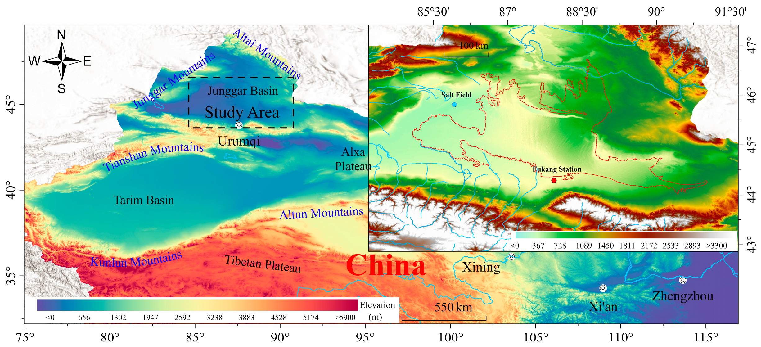
2.1. Study Area
2.2. Datasets
2.2.1. Remote Sensing Data
2.2.2. Ground–Measured Data
2.2.3. Data Processing
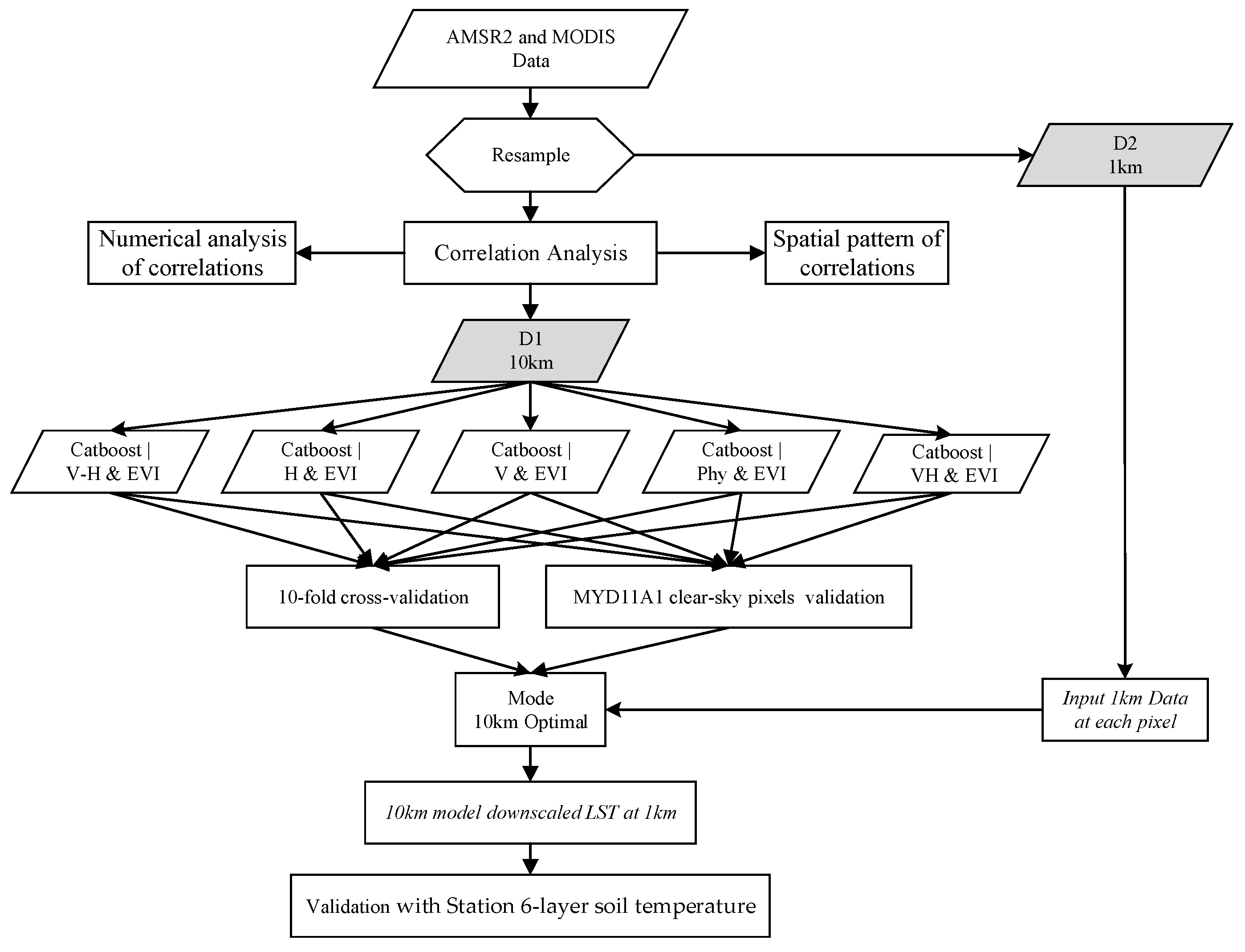
- (1)
- AMSR–2 and MODIS data were resampled to 10 km × 10 km (D1). Then, MYD11A1 pixels with quality average LST error ≤ 1 K were selected to match AMSR–2 microwave BT data and MYD13A2 vegetation index data.
- (2)
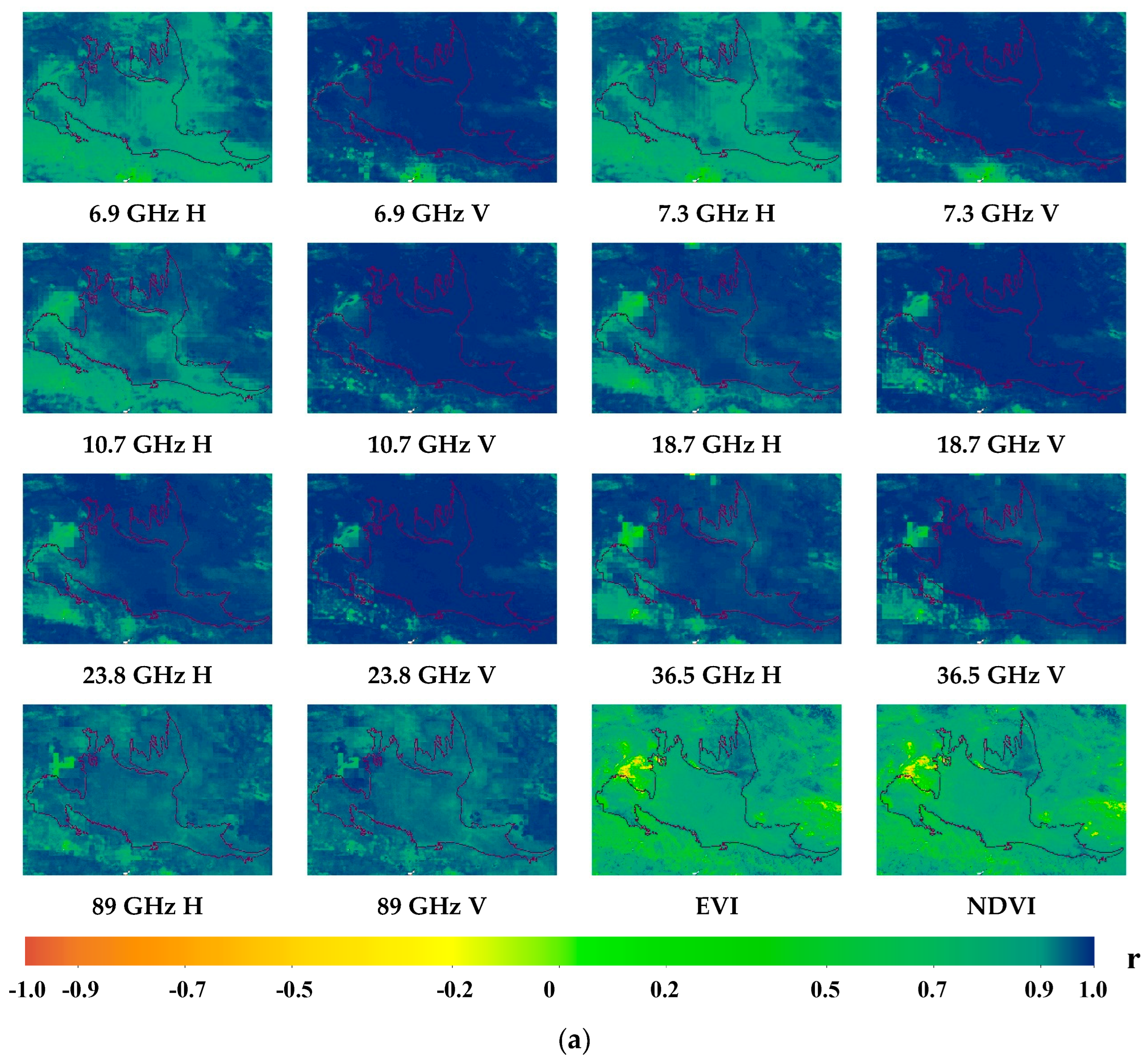
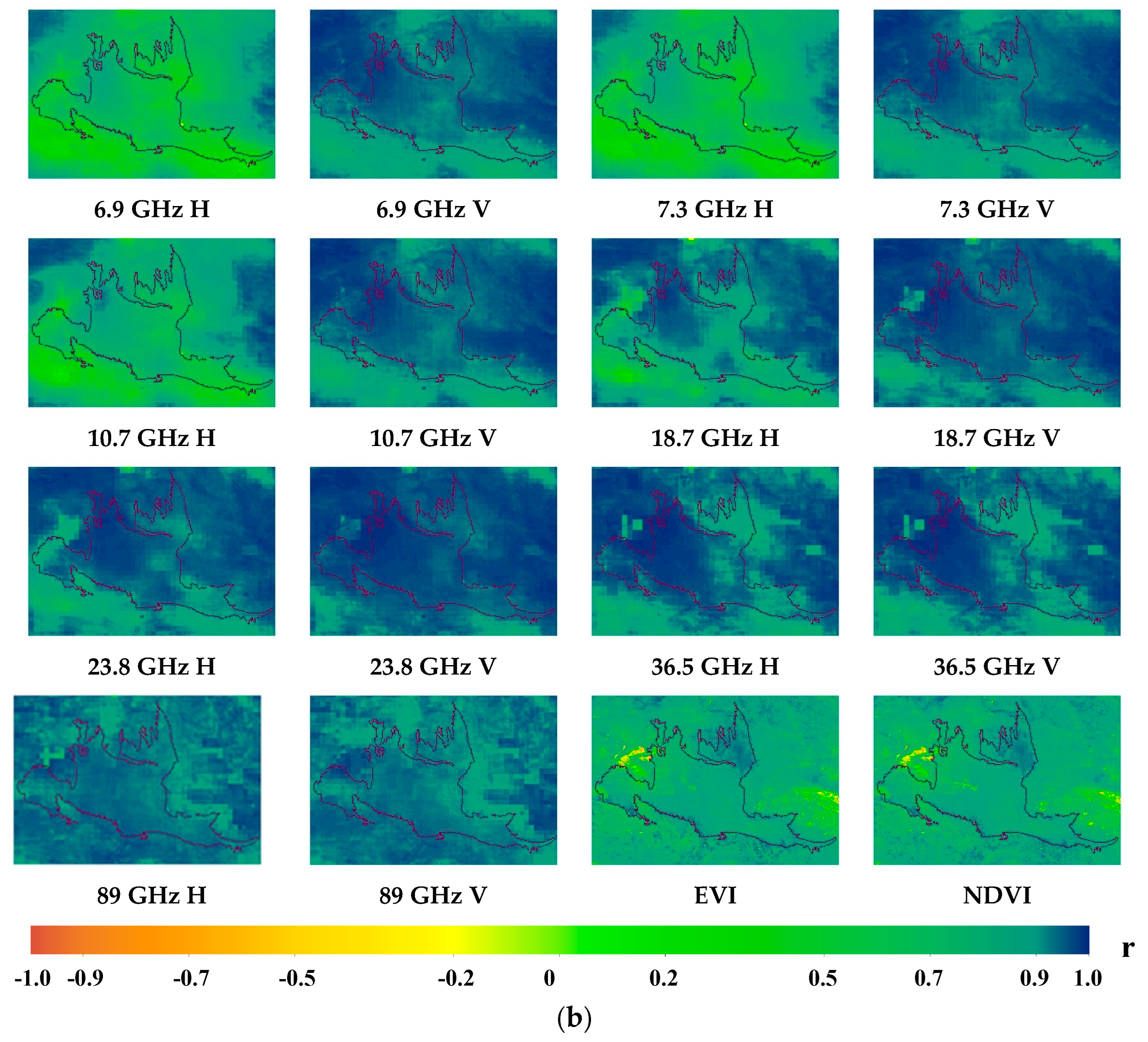
- The spatial correlation of the feature vectors was statistically analyzed. In order to obtain the spatial pattern of correlation coefficients (r) and probability (p) for each feature vector, 14 BTs and 2 vegetation indices were correlated with MYD11A1 data at a resolution of 10 km. The frequency distribution statistics of the correlation coefficients were calculated. On this basis, the frequency distribution characteristics and spatial characteristics of the correlation between each feature vector and LST data were analyzed.
- (3)
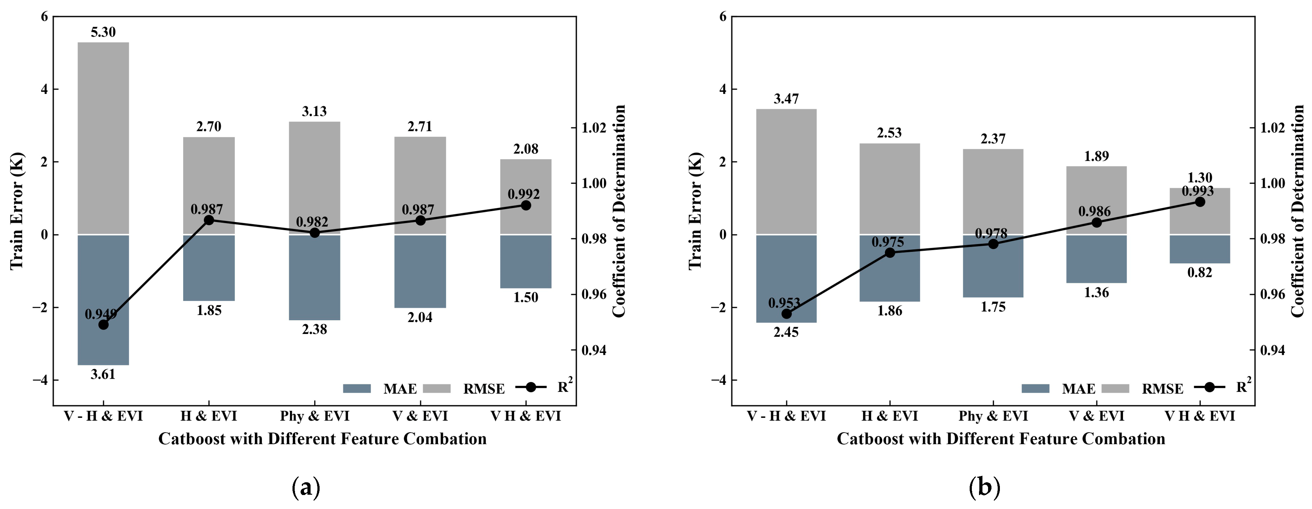
- Downscaled combinations of feature vectors were constructed. Based on the statistical analysis of correlation and the research studies of previous scholars, feature vector combinations were selected to train the Catboost model. The feature combinations were 7–channel algorithm [24] (difference between vertical polarization and horizontal polarization (V–H)), horizontal polarization combination [42] (7 horizontally polarized channels (H)), vertical polarization combination [42] (7 vertically polarized channels (V)), semi–empirical combination [32] (36.5 V/36.5 V–23.8 V/36.5 V–18.7 H/89 V GHz (Phy)), and full channel combination [42] (14 channels (VH)), respectively. The five microwave vector combinations were combined with vegetation indices to train five models of machine learning. The five models were initially evaluated using “10–fold cross–validation” to avoid overfitting [58,59,60].
- (4)
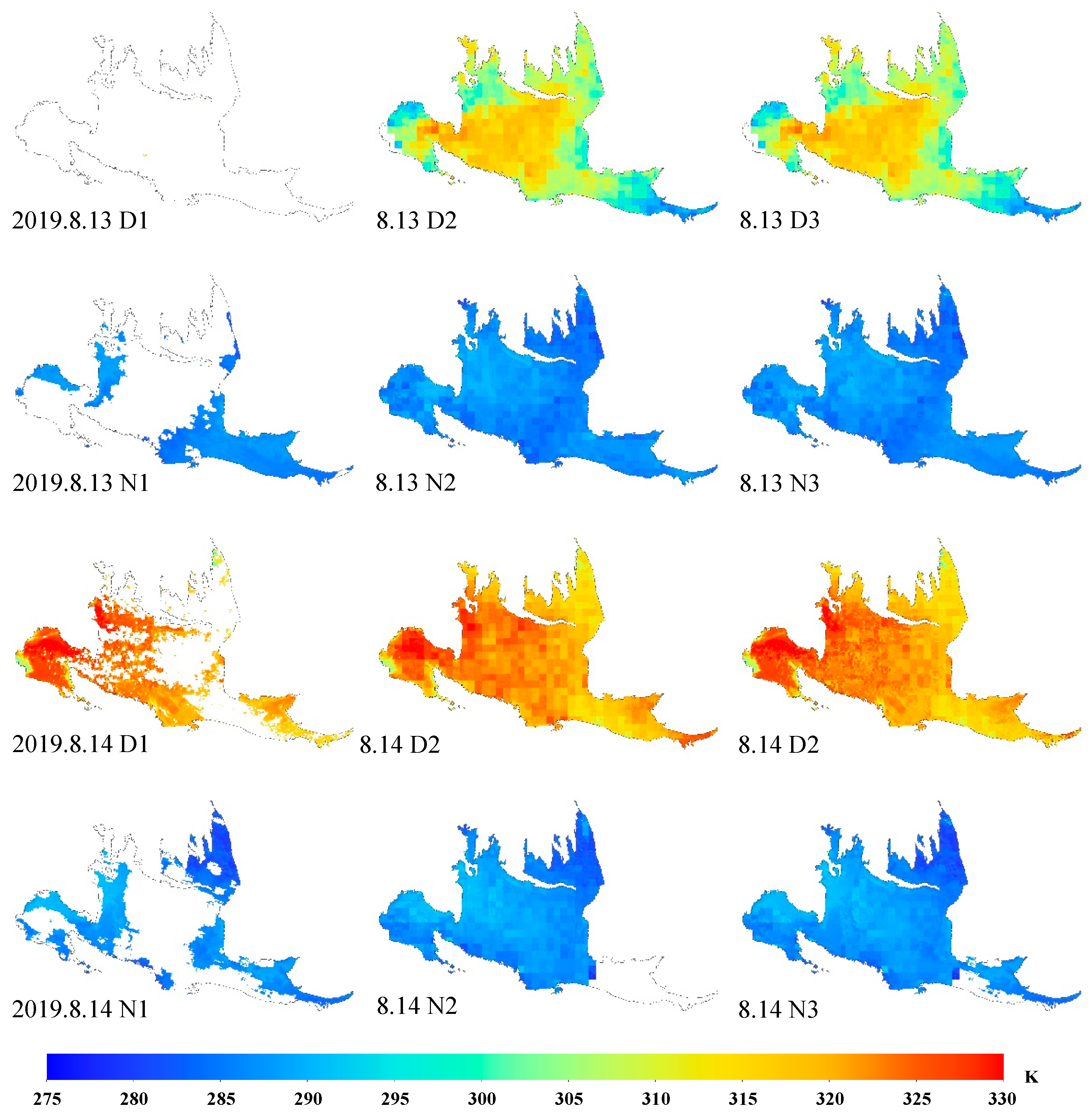
- Passive microwave BT data were resampled to 1 km (D2) using the nearest neighbor algorithm. Then, the 1 km MYD13A3 vegetation index data of the corresponding pixels were composed of five sets of feature vectors, which were input to the five machine learning models at 10 km resolution, respectively. The output 1 km pixels were the passive microwave surface temperature downscaling results.
- (5)
- MYD11A1 quality average LST error ≤1 K clear–sky pixels were selected to assess the consistency of downscaled surface temperature and MODIS data. Ten–fold cross–validation and MODIS validation were used to determine which was the optimal combination of downscaling feature vectors for the LST of a semi–heterogeneous underlying surface.
- (6)
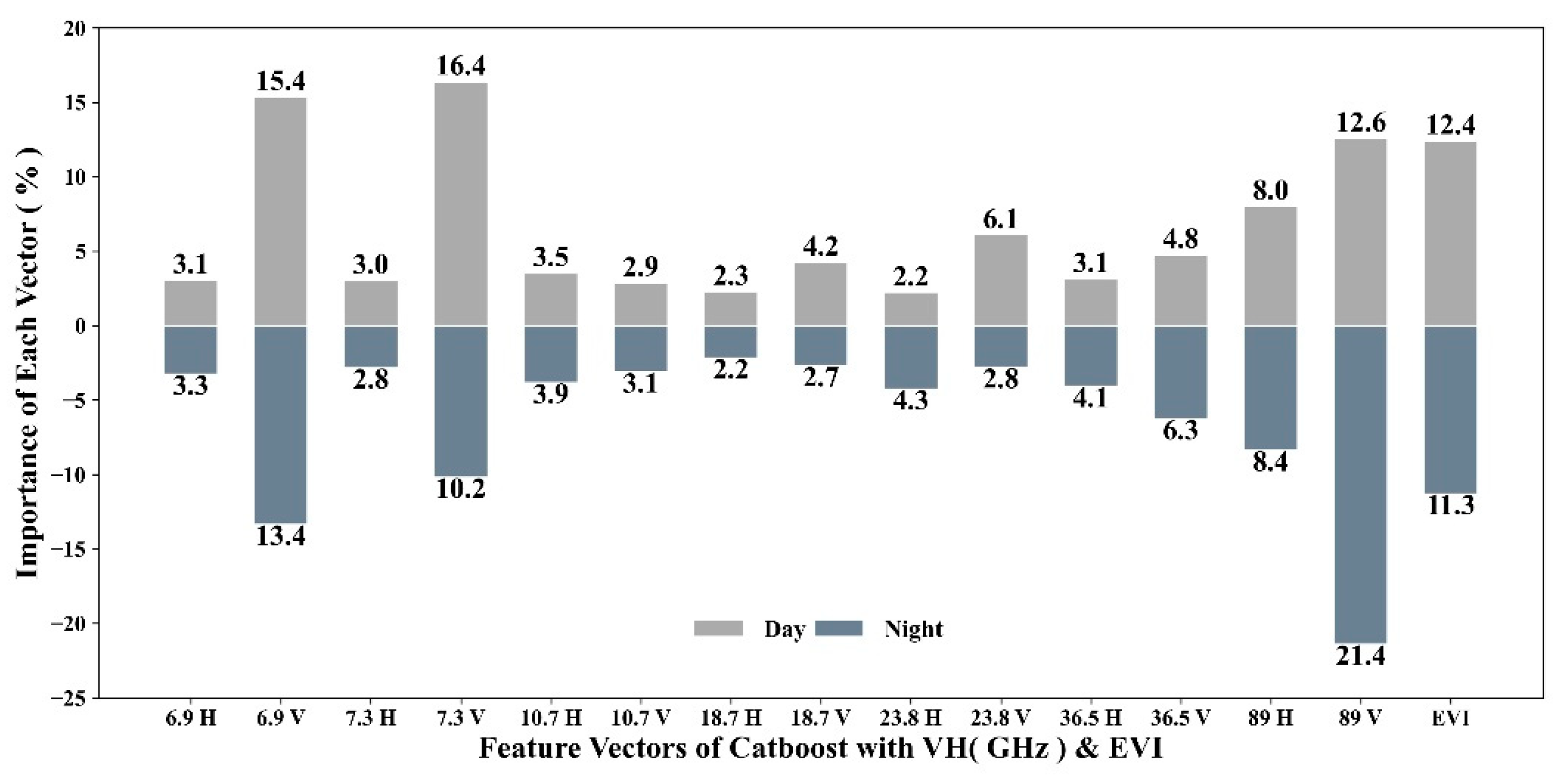
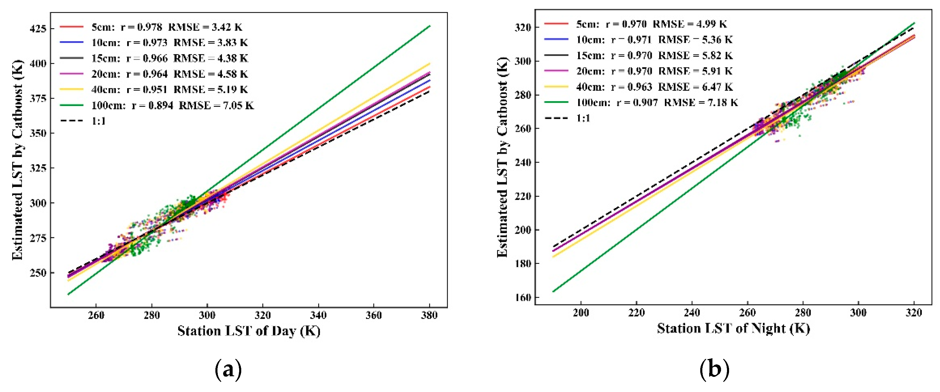
- Six–layer soil temperature data from Fukang station were selected for accuracy verification both to determine the correlation between soil temperature and passive microwave LST downscaling for each layer and to evaluate the optimal model. The importance of each feature vector in the optimal model was also summarized and analyzed in this last step.

2.3. Methods
2.3.1. Microwave Radiation Transmission Theory—Radiative Transmission Model for Microwave Surface Temperature Inversion
2.3.2. Categorical Boosting—Catboost
2.3.3. Validation Methods
3. Result
3.1. Correlation Statistical Analysis of Feature Vectors and LST
3.2. Ten–Fold Cross–Validation of Catboost for Five Feature Vector Combinations
3.3. Intercomparison and Analysis of LST Downscaling Results Based on Catboost
3.4. Microwave Surface Temperature Correlation Analysis Based on Six–Layer Ground Temperature Data
3.5. Catboost–Based, Diurnal, All–Weather Surface Temperature Products
4. Discussion
5. Conclusions
- (1)
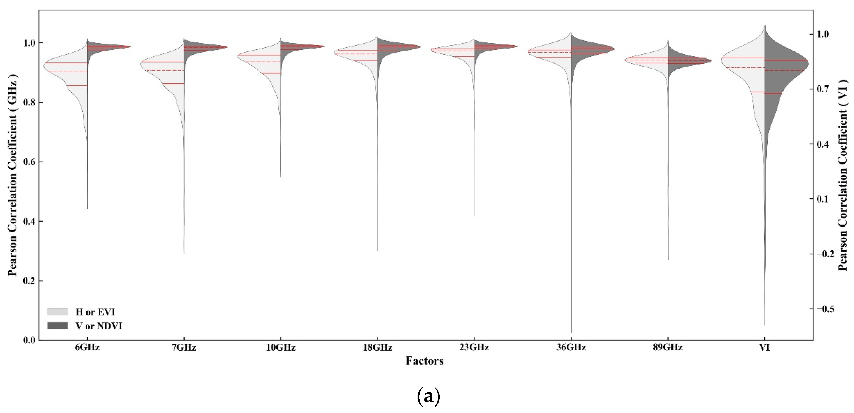
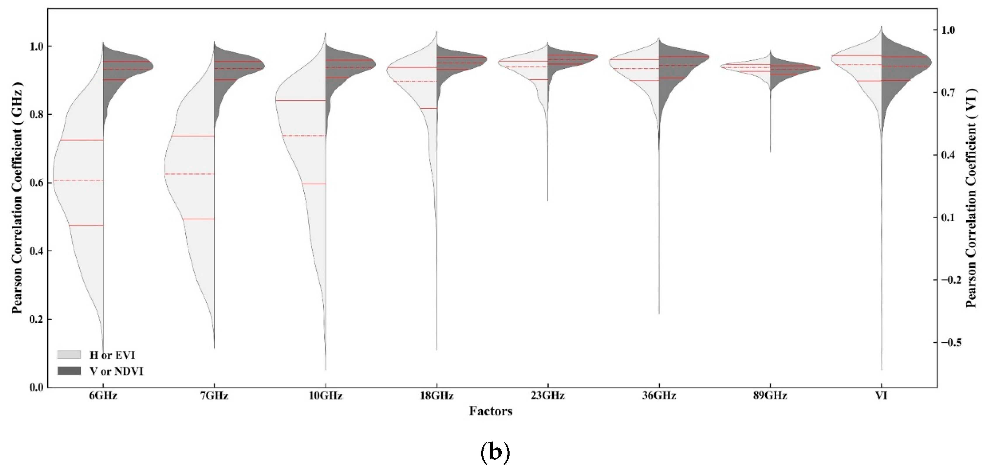
- The correlation coefficients between the feature vectors and LST of the semi–homogeneous underlying surface differed significantly from those of the surrounding oases, with the difference being more pronounced for daytime data. Specifically, the correlation coefficient of the semi–homogeneous underlying surface was high, while that of the surrounding oases was low. Moreover, we observed that the correlations between vertically polarized BT and LST were higher than those of horizontal polarization at the same frequency. As the frequency increased, the differences between the BT–LST correlation with horizontal polarization and that with vertical polarization at the same frequency became smaller.
- (2)
- Our ten–fold cross–validation results revealed that the Catboost model based on VH exhibited the best stability, with daytime R2, MAE, and RMSE mean values of 0.992, 1.50 K, and 2.08 K, respectively, and nighttime R2, MAE, and RMSE mean values of 0.993, 0.82 K, and 1.30 K, respectively. These results indicate that the Catboost model based on VH established the mapping relationship between passive microwave BT and LST more accurately than the other four classical models.
- (3)
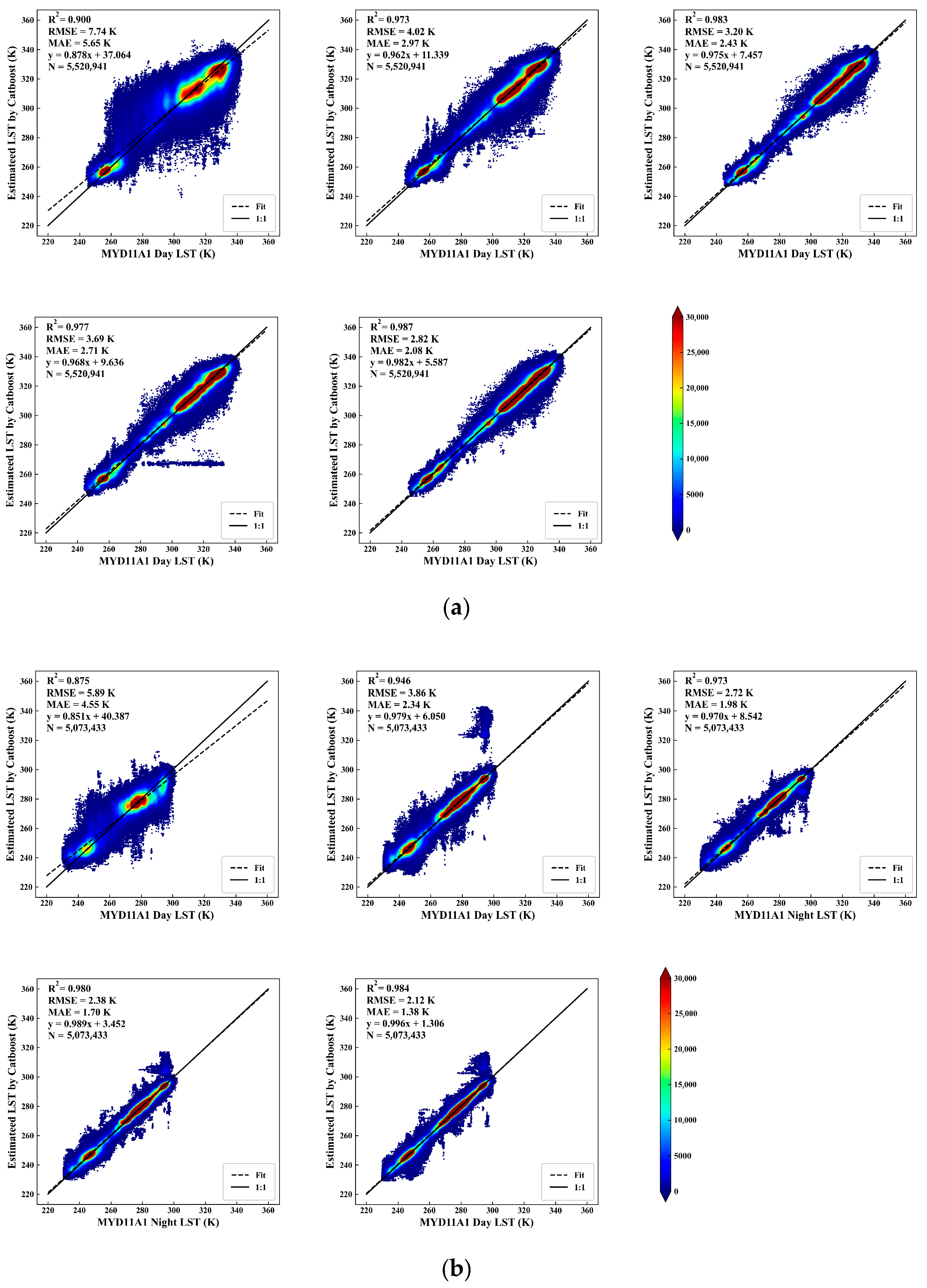
- Validation using MYD11A1 data revealed that LST downscaled with the Catboost model based on VH and EVI had the highest accuracy, with daytime and nighttime R2 of 0.987 and 0.984, RMSE of 2.82 K and 2.12 K, and MAE of 2.08 K and 1.38 K, respectively. Furthermore, we validated the downscaled LST data using the six–layer soil temperature data of the site, which showed a highly significant, positive correlation with all six–layer soil temperature data of the site. However, the correlation coefficients (r) generally showed a decreasing trend with increasing depth, while RMSE showed an increasing trend.
Author Contributions
Funding
Data Availability Statement
Acknowledgments
Conflicts of Interest
References
- Townshend, J.R.G.; Justice, C.O.; Skole, D.; Malingreau, J.P.; Cihlar, J.; Teillet, P.; Sadowski, F.; Ruttenberg, S. The 1 km resolution global data set: Needs of the International Geosphere Biosphere Programme. Int. J. Remote Sens. 1994, 15, 3417–3441. [Google Scholar] [CrossRef]
- Li, Z.L.; Wu, H.; Duan, S.B.; Zhao, W.; Ren, H.; Liu, X.; Leng, P.; Tang, R.; Ye, X.; Zhu, J.; et al. Satellite Remote Sensing of Global Land Surface Temperature: Definition, Methods, Products, and Applications. Rev. Geophys. 2023, 61, e2022RG000777. [Google Scholar] [CrossRef]
- Pérez-Planells, L.; Niclòs, R.; Puchades, J.; Coll, C.; Göttsche, F.-M.; Valiente, J.A.; Valor, E.; Galve, J.M. Validation of Sentinel–3 SLSTR Land Surface Temperature Retrieved by the Operational Product and Comparison with Explicitly Emissivity–Dependent Algorithms. Remote Sens. 2021, 13, 2228. [Google Scholar] [CrossRef]
- Faqe Ibrahim, G. Urban land use land cover changes and their effect on land surface temperature: Case study using Dohuk city in the Kurdistan Region of Iraq. Climate 2017, 5, 13. [Google Scholar] [CrossRef]
- Kimothi, S.; Thapliyal, A.; Gehlot, A.; Aledaily, A.N.; Bilandi, N.; Singh, R.; Malik, P.K.; Akram, S.V. Spatio–temporal fluctuations analysis of land surface temperature (LST) using Remote Sensing data (LANDSAT TM5/8) and multifractal technique to characterize the urban heat Islands (UHIs). Sustain. Energy Technol. Assess. 2023, 55, 102956. [Google Scholar] [CrossRef]
- Maffei, C.; Alfieri, S.; Menenti, M. Relating spatiotemporal patterns of forest fires burned area and duration to diurnal land surface temperature anomalies. Remote Sens. 2018, 10, 1777. [Google Scholar] [CrossRef]
- Wan, Z.; Wang, P.; Li, X. Using MODIS Land Surface Temperature and Normalized Difference Vegetation Index products for monitoring drought in the southern Great Plains, USA. Int. J. Remote Sens. 2010, 25, 61–72. [Google Scholar] [CrossRef]
- Shen, Y.; Shen, H.; Cheng, Q.; Zhang, L. Generating Comparable and Fine–Scale Time Series of Summer Land Surface Temperature for Thermal Environment Monitoring. IEEE J. Sel. Top. Appl. Earth Obs. Remote Sens. 2021, 14, 2136–2147. [Google Scholar] [CrossRef]
- Sun, H.; Chen, Y.; Gong, A.; Zhao, X.; Zhan, W.; Wang, M. Estimating mean air temperature using MODIS day and night land surface temperatures. Appl. Clim. 2014, 118, 81–92. [Google Scholar] [CrossRef]
- Tajfar, E.; Bateni, S.M.; Lakshmi, V.; Ek, M. Estimation of surface heat fluxes via variational assimilation of land surface temperature, air temperature and specific humidity into a coupled land surface–atmospheric boundary layer model. J. Hydrol. 2020, 583, 124577. [Google Scholar] [CrossRef]
- Kalma, J.D.; McVicar, T.R.; McCabe, M.F. Estimating land surface evaporation: A review of methods using remotely sensed surface temperature data. Surv. Geophys. 2008, 29, 421–469. [Google Scholar] [CrossRef]
- Wang, K.; Li, Z.; Cribb, M. Estimation of evaporative fraction from a combination of day and night land surface temperatures and NDVI: A new method to determine the Priestley–Taylor parameter. Remote Sens. Environ. 2006, 102, 293–305. [Google Scholar] [CrossRef]
- Liu, M.; Tang, R.; Li, Z.; Maofang, G.; Yunjun, Y. Progress of data-driven remotely sensed retrieval methods and products on land surface evapotranspiration. Natl. Remote Sens. Bull. 2021, 25, 1517–1537. [Google Scholar]
- Zhao, W.; Wen, F.; Wang, Q.; Sanchez, N.; Piles, M. Seamless downscaling of the ESA CCI soil moisture data at the daily scale with MODIS land products. J. Hydrol. 2021, 603, 126930. [Google Scholar] [CrossRef]
- Neteler, M. Estimating daily land surface temperatures in mountainous environments by reconstructed MODIS LST data. Remote Sens. 2010, 10, 333–351. [Google Scholar] [CrossRef]
- Li, Z.; Tang, B.; Wu, H.; Ren, H.; Yan, G.; Wan, Z.; Trigo, I.F.; Sobrino, J.A. Satellite–derived land surface temperature: Current status and perspectives. Remote Sens. Environ. 2013, 131, 14–37. [Google Scholar] [CrossRef]
- Caselles, V.; Coll, C.; Valor, E. Land surface emissivity and temperature determination in the whole HAPEX–Sahel area from AVHRR data. Int. J. Remote Sens. 1997, 18, 1009–1027. [Google Scholar] [CrossRef]
- Jimenez-Munoz, J.C.; Cristobal, J.; Sobrino, J.A.; Soria, G.; Ninyerola, M.; Pons, X.; Pons, X. Revision of the single–channel algorithm for land surface temperature retrieval from Landsat thermal–infrared data. IEEE Trans. Geosci. Remote Sens. 2009, 47, 339–349. [Google Scholar] [CrossRef]
- Duan, S.-B.; Li, Z.-L.; Wang, C.; Zhang, S.; Tang, B.-H.; Leng, P.; Gao, M.-F. Land–surface temperature retrieval from Landsat 8 single–channel thermal infrared data in combination with NCEP reanalysis data and ASTER GED product. Int. J. Remote Sens. 2018, 40, 1763–1778. [Google Scholar] [CrossRef]
- Mao, K.; Shi, J.; Tang, H.; Li, Z.L.; Wang, X.; Chen, K.S. A Neural Network Technique for Separating Land Surface Emissivity and Temperature From ASTER Imagery. IEEE Trans. Geosci. Remote Sens. 2008, 46, 200–208. [Google Scholar] [CrossRef]
- Chen, X.-Z.; Chen, S.-S.; Zhong, R.-F.; Su, Y.-X.; Liao, J.-S.; Li, D.; Han, L.-S.; Li, Y.; Li, X. A semi–empirical inversion model for assessing surface soil moisture using AMSR–E brightness temperatures. J. Hydrol. 2012, 456–457, 1–11. [Google Scholar] [CrossRef]
- He, W.; Chen, H.; Li, J. Development of land surface microwave emissivity retrieval using satellite observations. Chin. J. Geophys. 2020, 63, 3573–3584. [Google Scholar] [CrossRef]
- Qian, B.; Lu, Q.; Yang, S.; Guan, Y. Review on microwave land surface emissivity by satellite remote sensing. Prog. Geophys. 2016, 31, 960–964. [Google Scholar]
- Sun, D.; Li, Y.; Zhan, X.; Houser, P.; Yang, C.; Chiu, L.; Yang, R. Land Surface Temperature Derivation under All Sky Conditions through Integrating AMSR–E/AMSR–2 and MODIS/GOES Observations. Remote Sens. 2019, 11, 1704. [Google Scholar] [CrossRef]
- Li, Y.; Wang, X.; Ma, Y.; Hu, G.; Gui, H.; Zhang, G. Downscaling land surface temperature through AMSR–2 passive microwave observations by Catboost semiempirical algorithms. Arid Zone Res. 2021, 38, 1637–1649. [Google Scholar] [CrossRef]
- Yongkang, L.; Wang, X.; Yanfei, M.; Bei, C.; Linan, Y.; Guanhong, Z. Downscaling Land Surface Temperature through AMSR–2 Observations by Using Machine Learning Algorithms. Remote Sens. Technol. Appl. 2022, 37, 474–487. [Google Scholar]
- Bechtel, B.; Zakšek, K.; Hoshyaripour, G. Downscaling Land Surface Temperature in an Urban Area: A Case Study for Hamburg, Germany. Remote Sens. 2012, 4, 3184–3200. [Google Scholar] [CrossRef]
- Hutengs, C.; Vohland, M. Downscaling land surface temperatures at regional scales with random forest regression. Remote Sens. Environ. 2016, 178, 127–141. [Google Scholar] [CrossRef]
- Li, W.; Ni, L.; Li, Z.L.; Duan, S.B.; Wu, H. Evaluation of Machine Learning Algorithms in Spatial Downscaling of MODIS Land Surface Temperature. IEEE J. Sel. Top. Appl. Earth Obs. Remote Sens. 2019, 12, 2299–2307. [Google Scholar] [CrossRef]
- Favrichon, S.; Prigent, C.; Jiménez, C. A Method to Downscale Satellite Microwave Land–Surface Temperature. Remote Sens. 2021, 13, 1325. [Google Scholar] [CrossRef]
- Liu, Z.; Schwartz, C.S.; Chen, Y.; Huang, X.-Y. Impact of Assimilating Microwave Radiances with a Limited–Area Ensemble Data Assimilation System on Forecasts of Typhoon Morakot. Weather Forecast. 2012, 27, 424–437. [Google Scholar] [CrossRef]
- Mao, K.; Shi, J.; Li, Z.; Qin, Z.; Li, M.; Xu, B. A Physical Statistical Algorithm for Inverting LST from Passive Microwave AMSR–E Data. Sci. Sin. 2006, 36, 1170–1176. [Google Scholar]
- Mao, K.; Wang, D.; Li, Z.; Zhang, L.; Zhou, Q.; Tang, H.; Li, D. A neural network method for retrieving land–surface temperature from AMSR–E data. Chin. High Technol. Lett. 2009, 19, 1195–1200. [Google Scholar]
- Weng, F.; Grody, N.C. Physical retrieval of land surface temperature using the special sensor microwave imager. J. Geophys. Res. Atmos. 1998, 103, 8839–8848. [Google Scholar] [CrossRef]
- Fily, M. A simple retrieval method for land surface temperature and fraction of water surface determination from satellite microwave brightness temperatures in sub–arctic areas. Remote Sens. Environ. 2003, 85, 328–338. [Google Scholar] [CrossRef]
- Gao, H.; Fu, R.; Dickinson, R.E.; Negron Juarez, R.I. A Practical Method for Retrieving Land Surface Temperature From AMSR–E Over the Amazon Forest. IEEE Trans. Geosci. Remote Sens. 2008, 46, 193–199. [Google Scholar] [CrossRef]
- McFarland, M.J.; Miller, R.L.; Neale, C.M.U. Land surface temperature derived from the SSM/I passive microwave brightness temperatures. IEEE Trans. Geosci. Remote Sens. 1990, 28, 839–845. [Google Scholar] [CrossRef]
- Holmes, T.R.H.; De Jeu, R.A.M.; Owe, M.; Dolman, A.J. Land surface temperature from Ka band (37 GHz) passive microwave observations. J. Geophys. Res. 2009, 114, D04113. [Google Scholar] [CrossRef]
- Njoku, E.G.; Li, L. Retrieval of land surface parameters using passive microwave measurements at 6–18 GHz. IEEE Trans. Geosci. Remote Sens. 1999, 37, 79–93. [Google Scholar] [CrossRef]
- Duan, S.-B.; Li, Z.-L.; Leng, P. A framework for the retrieval of all–weather land surface temperature at a high spatial resolution from polar–orbiting thermal infrared and passive microwave data. Remote Sens. Environ. 2017, 195, 107–117. [Google Scholar] [CrossRef]
- Xu, F.; Fan, J.; Yang, C.; Liu, J.; Zhang, X. Reconstructing all–weather daytime land surface temperature based on energy balance considering the cloud radiative effect. Atmos. Res. 2022, 279, 106397. [Google Scholar] [CrossRef]
- Tan, J.; Esmaeel, N.; Mao, K.; Shi, J.; Li, Z.; Xu, T.; Yuan, Z. Deep Learning Convolutional Neural Network for the Retrieval of Land Surface Temperature from AMSR2 Data in China. Sensors 2019, 19, 2987. [Google Scholar] [CrossRef]
- Prokhorenkova, L.; Gusev, G.; Vorobev, A.; Dorogush, A.V.; Gulin, A. CatBoost: Unbiased boosting with categorical features. arXiv 2018, arXiv:1706.09516. [Google Scholar]
- Huang, G.; Wu, L.; Ma, X.; Zhang, W.; Fan, J.; Yu, X.; Zeng, W.; Zhou, H. Evaluation of CatBoost method for prediction of reference evapotranspiration in humid regions. J. Hydrol. 2019, 574, 1029–1041. [Google Scholar] [CrossRef]
- Zhang, K.; Schölkopf, B.; Muandet, K.; Wang, Z. Domain adaptation under target and conditional shift. In Proceedings of the International Conference on Machine Learning, Atlanta, GA, USA, 16–21 June 2013; pp. 819–827. [Google Scholar]
- Diao, L.; Niu, D.; Zang, Z.; Chen, C. Short–term Weather Forecast Based on Wavelet Denoising and Catboost. In Proceedings of the 2019 Chinese Control Conference (CCC), Guangzhou, China, 27–30 July 2019; pp. 3760–3764. [Google Scholar]
- Kim, H.; Park, S.; Park, H.-J.; Son, H.-G.; Kim, S. Solar Radiation Forecasting Based on the Hybrid CNN–CatBoost Model. IEEE Access 2023, 11, 13492–13500. [Google Scholar] [CrossRef]
- Kampaktsis, P.N.; Siouras, A.; Doulamis, I.P.; Moustakidis, S.; Emfietzoglou, M.; Van den Eynde, J.; Avgerinos, D.V.; Giannakoulas, G.; Alvarez, P.; Briasoulis, A. Machine learning-based prediction of mortality after heart transplantation in adults with congenital heart disease: A UNOS database analysis. Clinical Transplantation 2023, 37, e14845. [Google Scholar] [CrossRef] [PubMed]
- Wei, X.; Rao, C.; Xiao, X.; Chen, L.; Goh, M. Risk assessment of cardiovascular disease based on SOLSSA–CatBoost model. Expert Syst. Appl. 2023, 219, 119648. [Google Scholar] [CrossRef]
- Gao, J.; Wang, Y.; Sayithajigul, M.; Liu, Y.; Zhao, X.; Yang, X.; Huo, W.; Yang, F.; Zhou, C. Characteristics of surface radiation budget in Gurbantunggut Desert. J. Desert Res. 2021, 41, 47–58. [Google Scholar]
- Wang, X.; Zhao, C.; Yang, R.; Li, J. Landscape pattern characteristics of desertification evolution in southern Gurbantunggut Desert. Arid Land Geogr. 2015, 38, 1213–1225. [Google Scholar] [CrossRef]
- Wang, X.; Li, B.; Zhang, Y. Stabilization of Dune Surface and Formation of Mobile Belt at The Top of Longitudinal Dunes in Gurbantonggut Desert, Xinjiang, China. J. Desert Res. 2003, 23, 126. [Google Scholar]
- Ji, F.; Ye, W.; Wei, W. Preliminary study on the formation causes of the fixed and semi–fixed dunes in gurbantonggut desert. Arid Land Geogr. 2000, 23, 32–36. [Google Scholar] [CrossRef]
- Duan, C.; Wu, L.; Wang, S.; He, L. Analysis of spatio–temporal patterns of ephemeral plants in the Gurbantünggüt Desert over the last 30 years. Acta Ecol. Sin. 2017, 37, 2642–2652. [Google Scholar]
- Xie, F. Chinese Academy of Sciences established Fukang Desert Ecological Station. Arid Zone Res. 1988, 1, 8. [Google Scholar] [CrossRef]
- Fukang Desert Ecosystem Observation Experiment Station, Chinese Academy of Sciences. Bull. Chin. Acad. Sci. 1998. Available online: http://www.bcas.cas.cn (accessed on 14 March 2023).
- Chen, L.; Wang, S.; Wang, L. Variation Characteristics and Influencing Factors of NOx and Ozone in Autumn in Fukang Region of Xinjiang. J. Arid Meteorol. 2012, 30, 345–352. [Google Scholar]
- Fushiki, T. Estimation of prediction error by using K–fold cross–validation. Stat. Comput. 2011, 21, 137–146. [Google Scholar] [CrossRef]
- Berrar, D. Cross–Validation. In Encyclopedia of Bioinformatics and Computational Biology; Elsevier: Amsterdam, The Netherlands, 2019; Volume 1, pp. 542–545. [Google Scholar]
- Wong, T.-T.; Yeh, P.-Y. Reliable accuracy estimates from k–fold cross validation. IEEE Trans. Knowl. Data Eng. 2019, 32, 1586–1594. [Google Scholar] [CrossRef]
- Zhang, Y.; Zhao, Z.; Zheng, J. CatBoost: A new approach for estimating daily reference crop evapotranspiration in arid and semi–arid regions of Northern China. J. Hydrol. 2020, 588, 125087. [Google Scholar] [CrossRef]
- Colliander, A.; Jackson, T.J.; Bindlish, R.; Chan, S.; Das, N.; Kim, S.B.; Cosh, M.H.; Dunbar, R.S.; Dang, L.; Pashaian, L.; et al. Validation of SMAP surface soil moisture products with core validation sites. Remote Sens. Environ. 2017, 191, 215–231. [Google Scholar] [CrossRef]
- Wang, W.; Liang, S.; Meyers, T. Validating MODIS land surface temperature products using long–term nighttime ground measurements. Remote Sens. Environ. 2008, 112, 623–635. [Google Scholar] [CrossRef]
- Yu, W.; Ma, M.; Wang, X.; Song, Y.; Tan, J. Validation of MODIS Land Surface Temperature Products Using Ground Measurements in the Heihe River Basin, China; SPIE: Washington, DC, USA, 2011; Volume 8174. [Google Scholar]
- Yu, W.; Ma, M. Validation of the MODIS Land Surface Temperature Products—A Case Study of the Heihe River Basin. Remote Sens. Technol. Appl. 2012, 26, 705–712. [Google Scholar]
- Duan, S.-B.; Li, Z.-L.; Li, H.; Göttsche, F.-M.; Wu, H.; Zhao, W.; Leng, P.; Zhang, X.; Coll, C. Validation of Collection 6 MODIS land surface temperature product using in situ measurements. Remote Sens. Environ. 2019, 225, 16–29. [Google Scholar] [CrossRef]
- Xu, S.; Cheng, J. A new land surface temperature fusion strategy based on cumulative distribution function matching and multiresolution Kalman filtering. Remote Sens. Environ. 2021, 254, 112256. [Google Scholar] [CrossRef]
- Basist, A.; Grody, N.C.; Peterson, T.C.; Williams, C.N. Using the Special Sensor Microwave/Imager to monitor land surface temperatures, wetness, and snow cover. J. Appl. Meteorol. Climatol. 1998, 37, 888–911. [Google Scholar] [CrossRef]
- Liang, S.; Wang, D.; Tao, X.; Cheng, J.; Yao, Y.; Zhang, X.; He, T. 2.12—Methodologies for Integrating Multiple High–Level Remotely Sensed Land Products. In Comprehensive Remote Sensing; Liang, S., Ed.; Elsevier: Oxford, UK, 2018; pp. 278–317. [Google Scholar]
- Zhong, Y.; Meng, L.; Wei, Z.; Yang, J.; Song, W.; Basir, M. Retrieval of All–Weather 1 km Land Surface Temperature from Combined MODIS and AMSR2 Data over the Tibetan Plateau. Remote Sens. 2021, 13, 4575. [Google Scholar] [CrossRef]
- Fu, P.; Xie, Y.; Weng, Q.; Myint, S.; Meacham-Hensold, K.; Bernacchi, C. A physical model–based method for retrieving urban land surface temperatures under cloudy conditions. Remote Sens. Environ. 2019, 230, 111191. [Google Scholar] [CrossRef]
- Shwetha, H.R.; Kumar, D.N. Prediction of high spatio–temporal resolution land surface temperature under cloudy conditions using microwave vegetation index and ANN. ISPRS J. Photogramm. Remote Sens. 2016, 117, 40–55. [Google Scholar] [CrossRef]
- Zhang, X.; Zhou, J.; Gottsche, F.-M.; Zhan, W.; Liu, S.; Cao, R. A Method Based on Temporal Component Decomposition for Estimating 1–km All–Weather Land Surface Temperature by Merging Satellite Thermal Infrared and Passive Microwave Observations. IEEE Trans. Geosci. Remote Sens. 2019, 57, 4670–4691. [Google Scholar] [CrossRef]
- Zhao, W.; Duan, S.-B. Reconstruction of daytime land surface temperatures under cloud–covered conditions using integrated MODIS/Terra land products and MSG geostationary satellite data. Remote Sens. Environ. 2020, 247, 111931. [Google Scholar] [CrossRef]
- Li, Y. A Comparison Study on Microwave Land Surface Temperature Downscaling Methods and Similarity Evaluation of Spatial Structure. Master’s Thesis, Xinjiang Agricultural University, Urumqi, China, 2021. [Google Scholar]
- Peng, J.; Loew, A.; Merlin, O.; Verhoest, N.E.C. A review of spatial downscaling of satellite remotely sensed soil moisture. Rev. Geophys. 2017, 55, 341–366. [Google Scholar] [CrossRef]


| AMSR–2 Passive Microwave Bright Temperature Data | MODIS Data | ||||
|---|---|---|---|---|---|
| Center Frequency (GHz) | Polarization Direction | Spatial Resolution (km) | Data Types | Spatial Resolution (km) | Dataset |
| 6.925/7.3 | V/H | 10 | MYD 11A1 | 1 | LST_Day_1 kmQC_Day |
| 10.65 | V/H | 10 | |||
| 18.7 | V/H | 10 | |||
| 23.8 | V/H | 10 | MYD 13A2 | 1 | 1 km_16_days_EVI1 km_16_days_NDVI |
| 36.5 | V/H | 10 | |||
| 89 | V/H | 5 | |||
Disclaimer/Publisher’s Note: The statements, opinions and data contained in all publications are solely those of the individual author(s) and contributor(s) and not of MDPI and/or the editor(s). MDPI and/or the editor(s) disclaim responsibility for any injury to people or property resulting from any ideas, methods, instructions or products referred to in the content. |
© 2023 by the authors. Licensee MDPI, Basel, Switzerland. This article is an open access article distributed under the terms and conditions of the Creative Commons Attribution (CC BY) license (https://creativecommons.org/licenses/by/4.0/).
Share and Cite
Li, Y.; Liu, Y.; Huang, W.; Yan, Y.; Tan, J.; He, Q. Applicability Assessment of Passive Microwave LST Downscaling over Semi–Homogeneous Desert Underlying Surface Based on Machine Learning. Remote Sens. 2023, 15, 2626. https://doi.org/10.3390/rs15102626
Li Y, Liu Y, Huang W, Yan Y, Tan J, He Q. Applicability Assessment of Passive Microwave LST Downscaling over Semi–Homogeneous Desert Underlying Surface Based on Machine Learning. Remote Sensing. 2023; 15(10):2626. https://doi.org/10.3390/rs15102626
Chicago/Turabian StyleLi, Yongkang, Yongqiang Liu, Wenjiang Huang, Yang Yan, Jiao Tan, and Qing He. 2023. "Applicability Assessment of Passive Microwave LST Downscaling over Semi–Homogeneous Desert Underlying Surface Based on Machine Learning" Remote Sensing 15, no. 10: 2626. https://doi.org/10.3390/rs15102626