Prediction Models of ≥2 MeV Electron Daily Fluences for 3 Days at GEO Orbit Using a Long Short-Term Memory Network

Abstract

Geostationary satellites are exposed to harsh space weather conditions, including ≥2 MeV electrons from the Earth’s radiation belts. To predict ≥2 MeV electron daily fluences at 75°W and 135°W at geostationary orbit for the following three days, long short-term memory (LSTM) network models have been developed using various parameter combinations. Based on the prediction efficiency (PE) values, the most suitable time step of inputs and best combinations of two or three input parameters of models for predictions are recommended. The highest PE values for the following three days with three input parameters were 0.801, 0.658 and 0.523 for 75°W from 1995 to August 2010, and 0.819, 0.643 and 0.508 for 135°W from 1999 to 2010. Based on yearly PE values, the performances of the above models show the solar cycle dependence. The yearly PE values are significantly inversely correlated with the sunspot number, and they vary from 0.606 to 0.859 in predicting the following day at 75°W from 1995 to 2010. We have proven that the poor yearly PE is related to relativistic electron enhancement events, and the first day of events is the most difficult to predict. Compared with previous models, our models are comparable to the top performances of previous models for the first day, and significantly improve the performance for second and third days.

1. Introduction

Geostationary (GEO) orbit is an orbit at an altitude of approximately 36,000 km above the equator. Satellites at GEO orbit are crucial for telecommunication, weather monitoring, navigation, broadcasting, and other applications. However, being located in the outer electron radiation belt, GEO satellites are exposed to harsh space weather conditions, including relativistic electrons from the Earth’s radiation belts, which can cause damage to the electronic components of satellites, leading to malfunctions or even complete failure [1,2,3,4,5,6,7]. The energetic electrons, especially those ≥2 MeV, are a major source of radiation that pose a threat to the safety and longevity of GEO satellites [8,9,10,11]. Accurately predicting ≥2 MeV electron daily fluences for the following three days at GEO orbit is one of the indispensable aspects of daily space environment forecasting. Therefore, developing accurate prediction models for ≥2 MeV electron daily fluences is critical to assess the potential risk of radiation damage to GEO satellites and improve our ability to predict and mitigate the effects of space weather events.

In the past few decades, significant advancements have been made in predicting daily fluences of relativistic electrons at the geosynchronous Earth orbit. Li et al. [12,13,14,15] established a theoretical model based on radial diffusion. Solar wind parameters, Dst, and historical ≥2 MeV electron daily fluences are used in this model to predict the average daily fluences of ≥2 MeV electrons for the following 2 days. Various statistical models have also been developed, such as the REFM [16,17], Low-E [18], Combo [18], KLM by Rigler et al. [19], NARMAX by Ukhorskiy et al. [20] and Boynton et al. [21], DRX by Lam [22], probabilistic forecast model by Miyoshi and Kataoka [23,24], geomagnetic pulsation model by He et al. [25], EOF by Li et al. [26], multivariate regression model by Potapov et al. [27], multivariate autoregressive model by Sakaguchi et al. [28], NICT by Zhong et al. [29], hourly EMD prediction model by Qian et al. [30], and SaRIF by Glauert et al. [31].

With the continuous maturation of artificial intelligence technology, machine learning methods are constantly being developed and have been rapidly implemented in all walks of life. They can establish the complex relationship between inputs and outputs through the learning of data samples. The machine learning methods have also been used to predict relativistic electron fluxes. For example, Koon and Gorney [32], Fukata et al. [33], Xue and Ye [34], Guo et al. [35], Ling et al. [36], Shin et al. [37], and Zhang et al. [38] used neural networks with various external parameters as inputs to predict the ≥2 MeV electron daily fluences on the following day. Some researchers, such as Wang et al. [39], used the support vector machine (SVM)) method to predict the ≥2 MeV electron daily fluences at GEO orbit.

Deep learning methods, one research directions in machine learning, have achieved rapid development in recent years and are being widely employed in various applications, including natural language processing, speech recognition, target recognition, classification, and other applications [40,41,42]. Hinton et al. [43] proposed the concept of deep learning in 2006, which is an artificial neural network with multiple hidden layers. One of the most popular deep learning methods is the long short-term memory network (LSTM), a type of recurrent neural network (RNN) designed to handle time series data. Wei et al. [44] applied LSTM to develop models for predicting ≥2 MeV electron daily fluences on the following day at GEO orbit.

The models mentioned above require external parameters as inputs to make accurate predictions. These parameters may include the consecutive data of ≥2 MeV electron daily fluences, solar wind parameters (such as solar wind speed, density, and dynamic pressure, interplanetary magnetic field, etc.), geomagnetic disturbance indices (such as ap, kp, Dst, and AE), and low- or medium-energy electron fluxes on the previous day or a few days. The models above mainly predict the ≥2 MeV electron daily fluence on the following day, less so for the second and third days, which bring difficulties for predicting the daily space environment.

In addition, most of the models above only used data from one satellite, such as the radial diffusion model [12,13,14,15], Combo [18], LOW-E [18], multivariate autoregressive model by Sakaguchi et al. [28], geomagnetic pulsation model by He et al. [25], and RBF by Guo et al. [35]. These models should be used to predict the ≥2 MeV electron daily fluences at a certain location in geostationary orbit, which is the data used for modelling. Some models use the data from multiple geostationary satellites at different longitudes and ignore the differences in ≥2 MeV electron daily fluences at different longitudes in geostationary orbit, such as REFM [16,17], DRX by Lam [22], probabilistic forecast model by Miyoshi and Kataoka [23,24], neural network model by Fukata et al. [33], SVM by Wang et al. [39], and NARMAX by Ukhorskiy et al. [20] and Boynton et al. [21].

The different ≥2 MeV electron daily fluences at different longitudes in GEO orbit has been researched researchers, such as Ling et al. [36], Shin et al. [37], Onsager et al. [45], Sun et al. [46] and Sun et al. [47]. Sun et al. [47] reported that the ratios of ≥2 MeV electron daily fluences (cm⁻²·sr⁻¹·day⁻¹) from GOES-10 at about 135°W to those from GOES-12 at about 75°W are mainly in the range of 1.0 to 4.0, with an average of 1.92. With the assumption that the solar wind and geomagnetic disturbance conditions are stable and unchanged, Sun et al. [46] calculated ≥2 MeV electron daily fluences at different longitudes in GEO orbit on the same day based on the AE8+IGRF+T96 model. The minimum and maximum values of ≥2 MeV electron fluences of the GEO satellites on every day of the year appear near 70°W and 170°W, respectively, with their ratios varying from 1.86 to 2.13 per year. According to Sun et al. [47], the ratios of ≥2 MeV electron daily fluences at 135°W and 75°W per year range from 1.63 to 1.79, with an average ratio of 1.71. The differences between ≥2 MeV electron daily fluences at different longitudes in GEO orbit are primarily influenced by magnetic latitudes [45,46]. This is due to an angle of around 11° between the magnetic axis and the Earth’s axis of rotation [48,49]. These studies highlight the importance of considering longitude differences in the data used to model and predict.

The efficiencies of these models mentioned above for predicting ≥2 MeV electron daily fluences on the following day mostly range from 0.60 to 0.90. It is often difficult to judge which model is better when only relying on the prediction efficiencies given by the model articles, because their testing data are usually different, including the period or length of testing data, the longitude corresponding to the testing data, and so on. These factors all affect the prediction efficiency.

In this study, we develop models to predict ≥2 MeV electron daily fluences at 75°W and 135°W in GEO orbit for the following three days using an LSTM network, evaluate the model’s performance for each year from 1995 to 2010, and analyse the variation in the prediction efficiencies over the whole solar cycle. The paper is organized as follows: the data, the LSTM network, and the model evaluation are introduced in Section 2. In Section 3.1, we use data from 1995 to August 2010 for 75°W and from 1999 to 2010 for 135°W to determine the best offset time for modelling. We develop the models to predict the ≥2 MeV electron daily fluences on the following day at 75°W and 135°W at GEO orbit, evaluate the performances of the models with various parameters as inputs by their prediction efficiencies (PE), and compare our models with other models in Section 3.2. The models with different combinations as inputs are developed for the prediction of ≥2 MeV electron daily fluences on the next second or third day at GEO orbit, and the best combination of inputs is selected in Section 3.3. The solar cycle variation of the prediction efficiency is discussed in Section 4, and a summary and conclusions of this research are given in Section 5.

2. Materials and Methods

2.1. Data and Processing

The data used in this work include ≥2 MeV electron fluxes, ≥10 MeV proton fluxes and magnetic field data from GOES satellites, geomagnetic disturbance indices, solar wind parameters, and magnetopause subsolar distances from 1995 to 2010.

GOES satellites are equipped with energetic particle sensors (EPSs) and magnetometers (MAGs), which can recorded ≥2 MeV electron fluxes, ≥10 MeV proton fluxes, and vector magnetic fields. The ≥2 MeV electron fluxes and total magnitude of the magnetic field (Ht) are recorded with a 1 min resolution, and ≥10 MeV proton fluxes are recorded with a 5 min resolution.

Sun et al. [47] showed GOES satellites are mostly around 135°W or 75°W, and ≥2 MeV electron daily fluences between 135°W and 75°W are different. In this study, the ≥2 MeV electron daily fluences at a 1 min resolution from GOES-08 and GOES-12 satellites at roughly 75°W between 1995 and 2010, and from GOES-10 and GOES-11 satellites at about 135°W between 1999 and 2010 are used. The data of GOES satellites are available from the National Environmental Information Center (NCEI) website.

High-energy electron fluxes from GOES satellites may be contaminated during solar proton events [1,31,50], so the data of ≥2 MeV electron fluxes are removed, when ≥10 MeV proton fluxes at GEO orbit are greater than 3 cm⁻²·s⁻¹·sr⁻¹. If there is less than one hour of poor data in one day, including missing data from GOES satellites and data with proton contamination, linear interpolation is used to complete the data, otherwise, the data for that day is marked as poor. Then the ≥2 MeV electron daily fluences from different GOES satellites are calculated and converted to log₁₀ (≥2 MeV electron daily fluences), abbreviated as log₁₀ (daily fluences). The poor data will be kept in the dataset but skipped during training to ensure data consistency. The final available data are plotted in Figure 1. Figure 1a shows the available ≥2 MeV electron daily fluences from GOES-08 at roughly 75°W between 1995 and 2002 and from GOES-12 at roughly 75°W between September 2003 and August 2010. Figure 1b displays the available ≥2 MeV electron daily fluences from GOES-10 and GOES-11 at about 135°W between 1999 and 2010. The day of available data in each year is plotted as blue curves in Figure 1a,b. The distribution of ≥10 MeV proton fluxes from 1995 to 2010 and the 13 month smoothed sunspot number as an indicator for the solar cycle are shown in Figure 1c. There are several solar proton events between 1998 and 2006, mainly concentrated in years of high solar activity. The other external parameters, including solar wind speed (Vsw), density (N), dynamic pressure (Pd), temperature (T), kp, AE, Dst, and magnetopause subsolar distance (R0) are plotted in Figure 1d–g, respectively. The solar wind parameters, R0 and AE index are recorded with a 1 min resolution. Dst index is recorded with a 1 h resolution, and kp index is recorded with a 3 h resolution.

As shown in Figure 2 of Sun et al. [47], the calibration consistency of ≥2 MeV electron fluxes among GOES-10, GOES-11 and GOES-12 satellites had been verified. Based on the same method, Figure 2a displays the data from GOES-10 (black dots) and GOES-08 (blue dots) at almost the same longitude, covering each other very well during June and August 2003, and Figure 2b shows the observations of both satellites at the same time. The red dashed line is y = x, indicating that the calibration is consistent. The green dashed line is the result of linear fitting and almost coincides with the red line. This proves that the calibrations of ≥2 MeV electron fluxes among GOES-10 and GOES-08 are consistent. Therefore, the calibrations of ≥2 MeV electron fluxes among GOES-08, GOES-10, GOES-11, and GOES-12 are all consistent.

Solar wind parameters include speed (Vsw), density (N), dynamic pressure (Pd), electric field (E), temperature (T), plasma beta (beta), and the total magnitude of interplanetary magnetic field (Bt), Bx, By, Bz components of interplanetary magnetic field (IMF) in the GSM coordinates. Geomagnetic disturbance indices consist of kp, AE and Dst. Solar wind parameters and AE index are recorded with a 1 min resolution. Dst index is recorded with a 1 h resolution, and kp index is recorded with a 3 h resolution. The solar wind parameters and geomagnetic disturbance indices are all from the OMNI database. The magnetopause subsolar distances, R0, are calculated using Lin et al. [51]’s model with a 1 min resolution based on the solar wind data from the OMNI database. Missing values are repaired by linear interpolation. The daily averaged values of these parameters are used as inputs when modelling, so the transmission time from the locations of the OMNI data to GEO orbit is not considered.

2.2. Long Short-Term Memory (LSTM) and the Parameters of the Model

A recurrent neural network (RNN) is a type of deep learning method. Its structure is similar to the ordinary feedforward neural network, but its neurons in the same layer are not only connected to the neurons in the next layer but also connected in order. In this way, it refers to not only the current input information, but also the information entered previously [52]. Due to the addition of the time dimension, RNN can preserve more input information and overcome the shortcomings of traditional neural networks.

The LSTM network can be regarded as a variant of the RNN [53,54,55]. It was originally proposed by Hochreiter and Schmidhuber [56] and perfected by Graves et al. [52,53]. LSTM inherits the advantages of the RNN, and introduces a gating mechanism, allowing the model to selectively remember or forget certain information during the learning process. It can overcome the gradient vanishing and explosion problem existing in RNNs when the input sequence is too long [57,58,59]. LSTM adds a structure called the “memory cell” (mc) to memorize past information, and is controlled by input, output, and forget gates that regulate the flow of historical information. This architecture is particularly effective for processing long-term sequences, making it well-suited for time series analysis and other applications [60,61].

The forget gate in LSTM is responsible for receiving the output from the previous cell states and determining what should be kept and forgotten. The input gate is used to decide how much content the current cell needs to remember. It searches for relevant information in the unit module and adds it as a supplement to the information discarded by the forget gate. Lastly, the output gate decides which part of the cell state can be output and processes it accordingly [61]. Further details can be found in Sofiyanti et al. [59].

Since LSTM with memory capabilities shows strong advantages in dealing with time series forecasting and non-linear mapping problems [62,63], we develop models using LSTM with TensorFlow as the deep learning framework and Keras as the application program interface (API). TensorFlow is an open-source software library for numerical computation using data flow graphs, and Keras is a deep learning library based on Python, initially created by François Chollet as part of the ONEIROS project back in 2015.

We built a five-layer LSTM network containing an input layer, three LSTM layers, and an output layer. Multiple LSTMs can be stacked on top of each other, where the first LSTM gives the intermediate hidden states as the input for the second LSTM, and so on. Compared with the mono-directional LSTM, multiple LSTMs perform better in the stability of prediction results. The loss function is the MSE (mean square error), the optimizer is the AdamOptimizer [64], and the learning rate (lr) is 1 × 10⁻⁴.

The parameters of the model were hand-picked using cross-validation and iteration. The numbers of neurons in the LSTM layers are 64, 32, and 16, respectively. The batch size of the training set is 64, and the number of epochs is 60. When the model performance stops improving on the validation set, indicating overfitting, the training of the models is stopped.

We use a ten-fold cross-validation to evaluate the performance and stability of the models. The training set is divided into 10 equally sized parts, one as the validation set, and the rest as the training set. A total of 10 training test processes were carried out, and the test set comprised other datasets. Finally, the mean values of the 10 cross-validations are used as the model results.

2.3. Model Evaluation

The model’s performance is evaluated by the prediction efficiency (PE) and the root-mean-square error (RMSE). They are defined as:

$$PE=1-{\displaystyle \frac{{\sum }_{i=1}^n{(m_i-p_i)}^2}{{\sum }_{i=1}^n{(m_i-\overline{m})}^2}},$$

(1)

$$RMSE=\sqrt{{\displaystyle \frac{1}{n}}\sum _{i=1}^n{(p_i-m_i)}^2},$$

(2)

where m_i and p_i are the ith observation and prediction, respectively, $\overline{m}$ is the mean value of all observation samples, and n is the total number of samples. The larger the PE or smaller the RMSE, the better the model’s performance. When the PE value is below 0, this indicates that the prediction effect is unfavourable. In this study, the m_i is the log₁₀ (daily fluences) from the GOES satellites and the p_i is the log₁₀ (daily fluences) predicted by the models. In addition, the linear correlation coefficient (LC) and the relative errors are also used to evaluate the model’s performance.

3. Results

3.1. The Selection of the Best Offset Time

The offset time is the length of the time series of the model inputs. For example, if the offset time is two days, the model will use the consecutive data in the last two days as the inputs. The historical ≥2 MeV electron daily fluences are the most important parameter for predicting ≥2 MeV electron daily fluences on the following days. Solar wind speed (Vsw) and Kp index are also the most common training parameters in previous models [16,17,20,26,28,30,35,36,39,44]. We only use log₁₀ (daily fluences) or the combination of log₁₀ (daily fluences) and Vsw or Kp as the input parameters to determine the most suitable time step.

The data of the log₁₀ (daily fluences) from GOES-08 and GOES-12 (75°W) during January 1995 and August 2010 and log₁₀ (daily fluences) from GOES-10 and GOES-11 (135°W) during 1999 and 2010 are used to select the best offset time. Figure 3 shows the PE values of the models with different offset times and different input parameters to predict the ≥2 MeV electron daily fluences at 75°W in the left panels and 135°W in the right panels at GEO orbit for the following three days. The offset time ranges from 1 to 10 days. The different colour curves correspond to the different inputs shown at the top of Figure 3. The hollow circles represent the average PE values of the 10 cross-validation models, and the error bars represent the standard deviation of the PE values. The latter reflects the stability, while the former reflects the performance of the model.

The best offset time for the models are different with different input combinations. For the prediction of the following day, the best offset time for the model with (F, Vsw) as the input for predicting the following day at 75°W and 135°W is four days, and that for the model with (F, Kp) as the input is two days. When the offset time exceeds two days, the PE values of most models grows slowly or gradually decreases with the increasing offset time, as shown in Figure 3a,d. In addition, the error bars of a two day offset time are also relatively small. Considering the computational cost and the stability of the models, two days are taken as the best offset time for predicting the following day. For the same reason, three days will be used for predicting the following second or third day. That is, the data from day $n-2$ to day n are used for the prediction of day $n+2$ or day $n+3$.

3.2. The LSTM Models for Predicting ≥2 MeV Electron Daily Fluences on the Following Day at GEO Orbit

3.2.1. The Development of the LSTM Models

In this section, the data during 1999 and 2009 from GOES-10 and GOES-11 are used to develop models predicting ≥2 MeV electron daily fluences on the following day at 135°W at GEO orbit by the LSTM network with different input parameters, and tested during 1999 and 2010. The data during January 1995 and August 2009 from GOES-08 and GOES-12 are used to develop models predicting ≥2 MeV electron daily fluences on the following day at 75°W at GEO orbit, and the annual data during January 1995 and August 2010 are used to evaluate the solar cycle variation of the model’s performances. The gap between January and August 2003 will be kept in the dataset but skipped when modelling.

The PE values of models in each year for 75°W (left panels) and 135°W (right panels) with different inputs are plotted in Figure 4. The PE values of the models only using log₁₀ (daily fluences) as the input to predict ≥2 MeV electron daily fluences on the following day (black dots) and the persistence model (red dots) for 135°W and 75°W are shown in Figure 4a and Figure 4d, respectively. The persistence model uses the value at the current time as the prediction in the next time step. It is worth noting that due to the data gap between January 2003 and August 2003 at 75°W, only four months of data are used to calculate the PE value in 2003 and eight months of data for the PE value in 2010. The performances of the models with the five best combinations of two and three parameters are shown in the second and third row panels of Figure 4, respectively. The top five combinations were determined by the average PE values of 10 cross-validation models during the whole test set. The different combinations are listed in the panels with different colours and the PE values of each model are plotted with the same colour. The log₁₀ (daily fluences) are abbreviated as F and the “Per” represents the persistence model. The dark blue curve in each panel is the 13 month smoothed sunspot number, corresponding to the coordinates on the right.

When only using the log₁₀ (daily fluences) of the past two days as the inputs to predict the following day, the PE values of the LSTM models for 75°W based on the data from 1995 to August 2010 and for 135°W based on the data from 1999 to 2010 are 0.731 and 0.748, respectively, better than 0.671 and 0.736 from the persistence models. Figure 4a,d shows that the performances of the LSTM models only using log₁₀ (daily fluences) as the inputs are quite different for different years. The PE value in each year varies between 0.435 and 0.839. The PE values in 2009 and 2010 at 135°W are the highest, 0.816 and 0.839, respectively. The LSTM model usually behaves a bit better than the persistence model for each year. In addition, during the periods between 1999 and 2010, the models for 135°W usually performed better than the models for 75°W, except in 2007.

When using log₁₀ (daily fluences) and one of the external parameters listed in Section 2.1 as the inputs, (F, Vsw) and (F, Kp) are usually the best combinations of our models for the prediction of the following day, as shown in Figure 4b,e. The PE values of the model for 75°W from 1995 to August 2010 are 0.771 with (F, Vsw) and 0.769 with (F, Kp), and for 135°W are 0.790 and 0.784, respectively. The RMSE values of the model for 75°W are 0.3903 with (F, Vsw) and 0.3935 with (F, Kp), and for 135°W are 0.3801 and 0.3867, respectively. In addition, T, R0, N, AE, and Pd as inputs also contribute to improving the model’s performances in comparison to models only using log₁₀ (daily fluences) as the input.

When using a combinations of three parameters, the model with (F, Vsw, Kp) as the inputs performed best at both 75°W and 135°W, with PE values of 0.801 from 1995 to August 2010 and 0.819 from 1999 to 2010. The other best combinations are (F, N, Kp), (F, Vsw, AE), (F, T, Kp), and (F, N, AE). Although the top five combinations are ranked differently at 75°W and 135°W, there are no obvious differences in PE values of the corresponding models. The RMSE values of the models for 75°W and 135°W with (F, Vsw, Kp) as the inputs are 0.3753 and 0.3655, respectively. Modelling with a combination of three parameters, the (F, Vsw, Kp) performed the best. This combination is commonly used by previous researchers.

The PE values of our LSTM models with top five combinations of two or three parameters for predicting ≥2 MeV electron daily fluences on the following day are shown in

Table 1. The PE values of our LSTM models with the top five combinations of two or three parameters to predict ≥2 MeV electron daily fluences for the following day.

Longitude	Year	The Combinations of Different Parameters	PE of LSTM Model with Different Combinations
75°W	1995–2010.08	F + Vsw	0.771
		F + Kp	0.769
		F + N	0.765
		F + T	0.764
		F + AE	0.758
135°W	1999–2010	F + Vsw	0.790
		F + Kp	0.784
		F + T	0.780
		F + R0	0.779
		F + Pd	0.778
75°W	1995–2010.08	F + Vsw + Kp	0.801
		F + N + Kp	0.801
		F + Vsw + AE	0.799
		F + T + Kp	0.795
		F + N + AE	0.792
135°W	1999–2010	F + Vsw + Kp	0.819
		F + Vsw + AE	0.818
		F + N + AE	0.815
		F + T + Kp	0.811
		F + N + Kp	0.810

. The best combinations are often ordered differently at 135°W or 75°W. The best combination of three parameters are frequently the combinations of solar wind parameters and geomagnetic indices. the findings show that some external parameters have significant impacts on the PE values. Vsw, Kp, N and AE are the most important external parameters when predicting the ≥2 MeV electron daily fluences for the following day.

Compared to the model only using log₁₀ (daily fluences) as the input for the prediction at 75°W (135°W), the PE value increases by 5.5% (5.6%) for the model with (F, Vsw) as the input, and 9.6% (9.5%) for the model with (F, Vsw, Kp) as the input. In addition, the RMSE value increases by 7.9% (7.8%) for the model with (F, Vsw) as the input, and 11.4% (11.4%) for the model with (F, Vsw, Kp) as the input. The models with combinations of (F, Vsw) and (F, Vsw, Kp) as the inputs perform well at 75°W and 135°W, which can be taken as the best combinations of two and three parameters as inputs for modelling, respectively.

The performances of all the above models for various input parameters for 75°W and 135°W, including the persistence model, show solar cycle dependence, inversely correlated PE values with sunspot number, and the models always perform better during low solar activity periods. The linear correlation coefficient (LC) between the PE values of the model at 135°W with (F, Vsw, Kp) as the inputs and the sunspot number is −0.79.

Figure 5 shows a comparison of ≥2 MeV electron daily fluences between the observations from GOES satellites and the predictions of the LSTM models with (F, Vsw) or (F, Vsw, Kp) as the inputs. The black dots in Figure 5a–d represent the ≥2 MeV electron daily fluences from the GOES satellites as shown in each panel. The red dots in Figure 5a,b are the predictions of the LSTM models with (F, Vsw) as the inputs at 75°W or 135°W, respectively, and the red dots in Figure 5c,d are the predictions of the LSTM models with (F, Vsw, Kp) as the inputs. The blue dashed lines in each panel indicate that the ≥2 MeV electron daily fluences are equal to 10⁸ cm⁻²·sr⁻¹·day⁻¹. The data in Figure 5a–d are plotted as fluence–fluence coordinates in Figure 5e–h with black dots on their right to show the linear relationship of the observations and model results. The red lines, y = x, indicate that the observations are completely consistent with the predictions.

As shown in Figure 5, the LC values of the ≥2 MeV electron daily fluences between the observations from the GOES satellites and the predictions of the LSTM models with (F, Vsw) as the inputs are 0.82 and 0.80 at 75°W and 135°W, respectively, and 0.85 and 0.82 for the LSTM models with (F, Vsw, Kp) as the inputs at 75°W and 135°W, respectively. In Figure 5c, the absolute relative errors of log₁₀ (daily fluences) from the predictions with (F, Vsw, Kp) are mainly within 10%, and the absolute relative errors are within 5% for 79.7% of the time. In Figure 5d, the absolute relative errors of log₁₀ (daily fluences) from the predictions with (F, Vsw, Kp) are within 5% for 77.1% of the time.

3.2.2. Comparisons with Different Models

It has been proved that the prediction efficiencies of ≥2 MeV electron daily fluences have solar cycle dependence; however, previous models are typically evaluated in one or several years rather than an entire solar cycle, and different models are usually evaluated in different years. Therefore, it is not our objective to evaluate which model is better according to the PE values provided by their articles.

In order to evaluate each model objectively, the PE value of our LSTM model with (F, Vsw, Kp) as the inputs is shown in

Table 2. A comparison of the prediction efficiencies of the ≥2 MeV electron daily fluences (+1 day) of the different models.

Model/Year	The Sunspot Number	LSTM Model for 75°W (135°W)	SVM Model by Wang et al. (2012) [39]	RBF Model by Guo et al. (2013) [35]	Geomagnetic Pulsation Model by He et al., 2013) [25]	Empirical Orthogonal Function Model by Li et al., 2017) [26]	LSTM Model by Wei et al. (2018) [44]	EMD Model by Qian et al., 2020) [30]
		F + Vsw + Kp	A Total of Five Parameters	F + Vsw + ap	F + Pi12 + Pc5	A Total of Eight Parameters	F + Vsw + Kp or F + R0 + Kp	A Total of Ten Parameters
1995	24.78	0.769
1996	12.56	0.827
1997	30.50	0.743
1998	85.79	0.785
1999	139.67	0.790 (0.812)
2000	169.89	0.607 (0.589)
2001	168.28	0.606 (0.586)						0.730
2002	160.48	0.646 (0.705)	0.670					0.810
2003	102.95	0.777 (0.678)			0.730	0.613		0.780
2004	66.29	0.790 (0.816)			0.620	0.673		0.810
2005	44.83	0.765 (0.787)			0.720	0.664		0.790
2006	26.05	0.859 (0.840)				0.762		0.830
2007	13.18	0.848 (0.779)
2008	4.21	0.837 (0.806)	0.710	0.776			0.833
2009	6.39	0.759 (0.886)		0.808			0.896
2010	26.19	0.833 (0.891)		0.882			0.911
1995–2010 (1999–2010)	67.62	0.801 (0.819)

for each year from 1995 to 2010. The PE values of the SVM model by Wang et al. [39], RBF model by Guo et al. [35], geomagnetic pulsation model by He et al. [25], EOF model by Li et al. [26], LSTM model by Wei et al. [44], and EMD model by Qian et al. [30] are also listed in Table 2. This allows us to compare the performance of our model with other models in the same year. In addition, it is possible to indirectly compare the performances of many earlier models. Other models mentioned in this article, such as the FLUXPRED [36] and REFM models [16,17], are not listed in Table 2, because these models did not predict during the same years as our models.

Table 2 lists the prediction efficiencies of ≥2 MeV electron daily fluences (+1 Day) of our models for 75°W and 135°W and previous models. The RBF model [35] and geomagnetic pulsation model [25] used the data from GOES-12 at 75°W; EOF [26] and EMD models [30] used the data from GOES-10 at 135°W; and the SVM [39] and LSTM models [44] used the data from 75°W and 135°W. By comparing the PE values of each model in the same longitude and the same year, our LSTM model performs better than the SVM model [39], geomagnetic pulsation model [25] and EOF model [26] in predicting the ≥2 MeV electron daily fluences for the following day, but worse than the RBF model by Guo et al. [35] in 2009 and 2010, the LSTM model by Wei et al. [44], and the EMD model by Qian et al. [30].

The PE values of the RBF model by Guo et al. [35] in 2009 and 2010 were relatively high, because they used data throughout both years and the abnormal data were repaired by linear interpolation. There are only 249 and 243 days of data available from September 2008 to August 2009 and from September 2009 to August 2010. If the same data as Guo et al. [35] is used, the PE values of our LSTM model in 2009 and 2010 are 0.858 and 0.889, respectively, higher than those of the RBF model. Wei et al. [44] obtained higher PE values due to a longer offset time. If the same offset time (5 days) as Wei et al. [44] is used, the PE values of our LSTM model in 2008, 2009 and 2010 are 0.847, 0.899 and 0.918, respectively.

Additionally, the EMD model developed by Qian et al. [30] is an hourly prediction model, which uses the summation to predict the daily fluences for the following day. Wei et al. [44] obtained higher resolution data containing more characteristics of the diurnal variation, ignored in the daily fluences or averaged values. The characteristics preserved by higher-resolution data will be learned by the networks, so the hourly prediction model performs better than the daily prediction model. The highest PE values of the daily fluences for the following day based on the hourly prediction model of the LSTM model by Wei et al. [44] reached 0.900 in 2008.

In general, the overall effect of the LSTM model is better than the traditional prediction models and our LSTM model may be used for the prediction of ≥2 MeV electron daily fluences for the following day at GEO orbit.

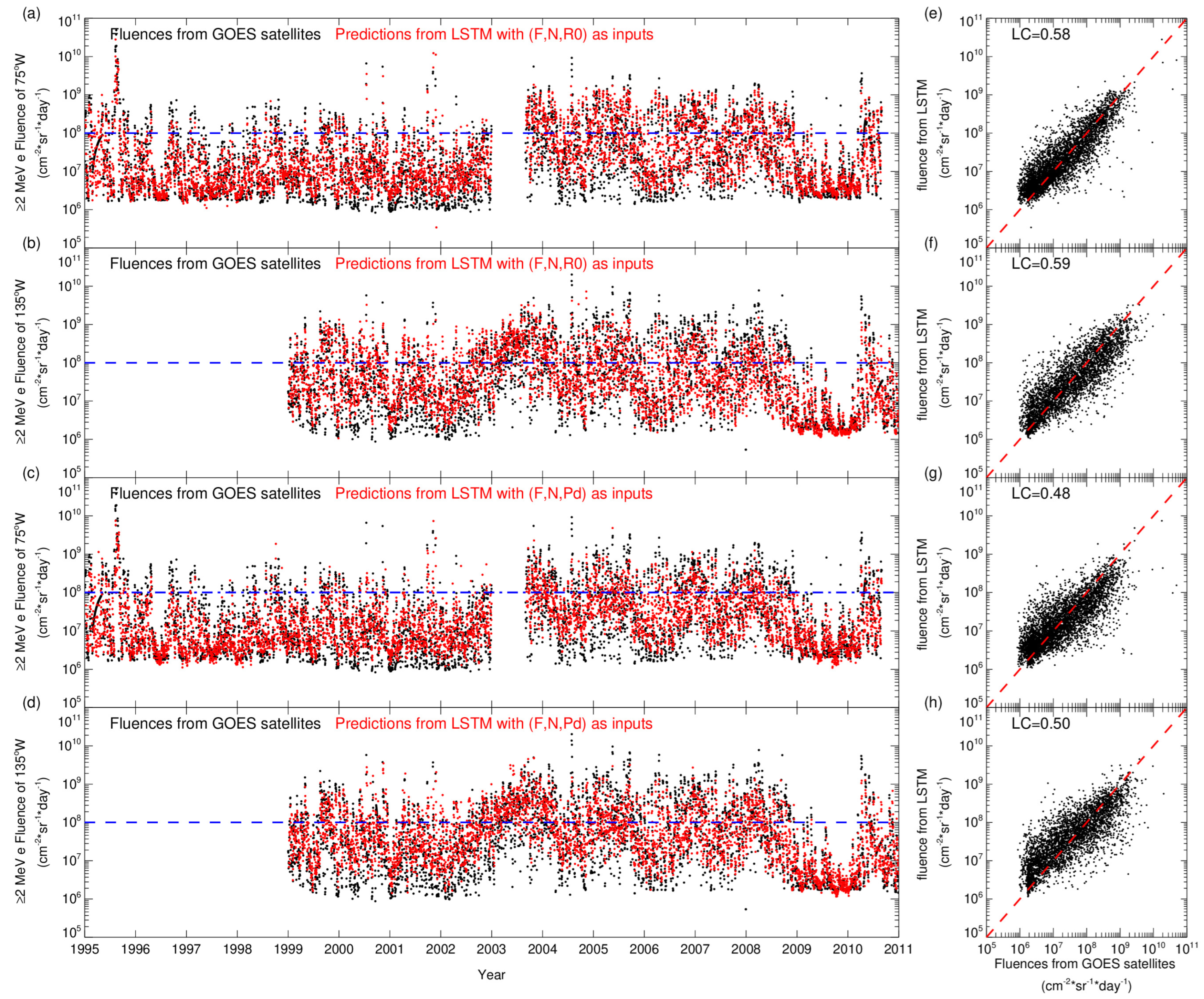
3.3. The LSTM Models for Predicting ≥2 MeV Electron Daily Fluences for the Following Second or Third Day at GEO Orbit

The previous prediction models primarily focused on the ≥2 MeV electron daily fluences on the following day and paid less attention to predicting further into the future. To test the impacts of different external factors and find models with the best combinations for daily space environment forecasting, we developed models to predict the ≥2 MeV electron daily fluences for the following second and third days. The datasets were the same as in Section 3.2.

The PE values of models in each year for 135°W (left panels) and 75°W (right panels) with different inputs for predicting the ≥2 MeV electron daily fluences on the second and third days are plotted in Figure 6 and Figure 7. The formats are the same as in Figure 4.

When only using log₁₀ (daily fluences) as the inputs for predicting the second or third days, the PE values of our models for 75°W based on the data from 1995 to August 2010 are 0.497 and 0.327, better than 0.342 and 0.076 from the persistence models, and they are 0.528 and 0.373 for 135°W based on the data from 1999 to 2010, better than 0.404 and 0.149 from the persistence models, respectively.

The performances of our LSTM models with the top five combinations of two or three parameters for predicting the ≥2 MeV electron daily fluences on the second or third days are shown in

Table 3. The performances of our LSTM models with the top five best combinations of two or three parameters for predicting ≥2 MeV electron daily fluences on the second or third days.

Prediction	Longitude	Year	The Combinations of Different Parameters	PE of LSTM Model with Different Combinations
For the second day	75°W	1995–2010.08	F + Vsw	0.605
			F + T	0.586
			F + Dst	0.580
			F + Bz	0.573
			F + N	0.550
	135°W	1999–2010	F + Vsw	0.608
			F + T	0.594
			F + N	0.543
			F + Bz	0.530
			F + Dst	0.528
For the third day	75°W	1995–2010.08	F + Vsw	0.461
			F + T	0.454
			F + Bz	0.410
			F + Dst	0.406
			F + N	0.401
	135°W	1999–2010	F + Vsw	0.475
			F + T	0.467
			F + Dst	0.397
			F + N	0.391
			F + Bz	0.387
For the second day	75°W	1995–2010.08	F + Vsw + N	0.658
			F + N + R0	0.651
			F + Vsw + Pd	0.649
			F + Vsw + R0	0.638
			F + N + Pd	0.632
	135°W	1999–2010	F + Vsw + AE	0.643
			F + N + R0	0.637
			F + Vsw + R0	0.632
			F + N + Pd	0.626
			F + Vsw + Kp	0.619
For the third day	75°W	1995–2010.08	F + N + Pd	0.523
			F + Vsw + R0	0.514
			F + Vsw + T	0.507
			F + Vsw + Dst	0.505
			F + Vsw + N	0.504
	135°W	1999–2010	F + N + Pd	0.508
			F + N + R0	0.504
			F + Vsw + N	0.501
			F + Vsw + R0	0.485
			F + Vsw + Dst	0.483

and Figure 6 and Figure 7. If only one external parameter is used as the input for predicting the second or third days, Vsw, T, Dst, N and Bz are the top five parameters in order based on the PE values during the test set, as listed in Table 3. (F, Vsw) and (F, T) are usually the better combinations of our models for predicting the second or third days. The PE values of our models with (F, Vsw) and (F, T) as the inputs are 0.605 and 0.586 at 75°W from 1995 to August 2010, and 0.608 and 0.594 at 135°W from 1999 to 2010, respectively. The RMSE values of the model with (F, Vsw) and (F, T) as the inputs for predicting the second day at 75°W are 0.5143 and 0.5262, and 0.5121 and 0.5137 for 135°W, separately.

If two external parameters are used as the input for predicting the second or third days, the best combinations are often ordered differently at 135°W and 75°W. Vsw, N, R0 and Pd are the most frequent external parameters in the top five best combinations for predicting the ≥2 MeV electron daily fluences on the second or third days, as shown in Figure 6c,f and Figure 7c,f and Table 3. The best combinations as inputs for predicting the second day are (F, Vsw, N) for 75°W, with a PE value of 0.658 from January 1995 to August 2010, and (F, Vsw, AE) for 135°W, with a PE value of 0.643 from 1999 to 2010. The second best combinations as the inputs for predicting the second day are both (F, N, R0), with a PE value of 0.651 at 75°W from January 1995 to August 2010, and 0.637 at 135°W from 1999 to 2010. The RMSE values of the model with (F, Vsw, N) and (F, N, R0) as the inputs for predicting the second day at 75°W are 0.4780 and 0.4821, and those for 135°W with (F, Vsw, AE) and (F, N, R0) as the inputs are 0.4851 and 0.4924, respectively. For the predictions of the third day, the models with (F, N, Pd) as inputs perform best for both 75°W and 135°W, with PE values of 0.523 at 75°W from January 1995 to August 2010 and 0.508 at 135°W from 1999 to 2010, and RMSE values of 0.5649 at 75°W and 0.5789 at 135°W.

When compared to the model only using log₁₀ (daily fluences) as the input, it is clear that some combinations with two or three parameters as the inputs can improve model performances. The highest PE value is 0.784 (three parameters) or 0.640 (two parameters) in 2007 at 75°W for predicting the second day, and 0.690 (three parameters) or 0.528 (two parameters) in 2010 at 135°W for predicting the third day. It can also be seen that the models with three parameters as inputs perform better than those with two parameters as inputs in general.

As listed in Table 3, the rankings of the top five combinations vary, but the discrepancies are not substantial. The models with the combinations of (F, N, R0) as inputs perform well for both 75°W and 135°W on the second day, and the models with the combinations of (F, N, Pd) as inputs perform well for both 75°W and 135°W on the third day. The performances of all the above models with various inputs for predicting the second or third days at 75°W and 135°W show solar cycle dependence, inversely correlated PE values with sunspot number, and the models always perform better during low solar activity periods.

The prediction results of the LSTM model for 75°W and 135°W with different combinations on the second and third days are shown in Figure 8. The format is the same as Figure 5. The black dots in each panel represent the available data from the GOES satellites, and the red dots in Figure 8a–d are the predictions of the LSTM model for 135°W or 75°W with the best combination of three parameters as the inputs. The inputs are (F, N, R0), (F, N, R0), (F, N, Pd), and (F, N, Pd) from top to bottom.

It is obvious that the PE values gradually decrease with the increase in forecast days. The predictions of the LSTM model for the following days are more consistent with the observations from the GOES satellites than those from the LSTM model for the second or third days. For the test data with (F, N, R0) as the inputs in Figure 8a,b, the absolute relative errors of log₁₀ (daily fluences) between the GOES satellites and the predictions are mainly within 10%. The absolute relative errors at 75°W are within 5% for 72.7% of the time, and those at 135°W are within 5% for 67.2% of the time. For the test data with (F, N, Pd) as inputs in Figure 8c,d, the absolute relative errors at 75°W are within 5% for 58.3% of the time, and those at 135°W are within 5% for 54.9% of the time. The absolute relative errors of the log₁₀ (daily fluences) greater than 10% mostly occur at the beginning and end of the relativistic electron enhancement events.

As mentioned before, the previous models paid less attention to predictions of the ≥2 MeV electron daily fluences on the second and third days. Ling et al. [36] developed the FLUXPRED model to predict the following three days. The PE values of the FLUXPRED and REFM models for predicting the ≥2 MeV electron daily fluences on the second day for 6-month intervals over the period 1998–2008 are 0.49 and 0.09, respectively, and those for the prediction of the third day are 0.31 and −0.04, respectively [36]. Our LSTM model performs better than those models in predicting the ≥2 MeV electron daily fluences on the second or third days.

4. Discussion

Based on the yearly PE values of the LSTM models in Section 3.2 and Section 3.3, the performances of the models to predict the ≥2 MeV electron daily fluences for the following three days at GEO orbit show solar cycle dependence, and the yearly PE values are significantly inversely correlated with the sunspot number. This inverse correlation is independent of the input parameters and the advance day of prediction, so it will be discussed below using the prediction model with (F, Vsw, Kp) as the inputs on the following day.

Figure 9a–c show the relationship between the PE values of the LSTM model for predicting the following day using (F, Vsw, Kp) as the input at 75°W (red dots) and 135°W (black dots) and the event number, the total number of days and the average duration of relativistic electron enhancement events in each year from 1995 to 2009, respectively. A relativistic electron enhancement event is identified by ≥2 MeV electron daily fluences higher than 10⁸ cm⁻²·sr⁻¹·day⁻¹. The black dotted curve in each panel is the result of the linear fitting. The number of relativistic electron enhancement events in each year at 75°W (red curves) and 135°W (black curves) from 1995 to 2009 is plotted in Figure 9d. The dark blue curve in Figure 9d is the 13-month smoothed sunspot number, corresponding to the coordinates on the right.

Figure 9a–c illustrates that the PE value in each year decreases with an increase in the event number or the total number of days of relativistic electron enhancement events. As the average duration of each relativistic electron enhancement event increases, the PE values gradually rise. That is, the PE values of the models for predicting the ≥2 MeV electron daily fluences are related to the relativistic electron enhancement events.

In order to know which stage of a relativistic electron enhancement event is the most difficult to predict, the PE values at different stages were compared. Figure 9e shows the PE values for the predictions of the following day at 135°W before the first day, on the first day, on the second day, on the last day and the day after the last day of the relativistic electron enhancement events in each year from 1999 and 2008. In each year these events are all greater than 10, as shown in Figure 9d. It is obvious that the first day of events are the most difficult to predict, as their PE values are significantly lower than the results of other days.

5. Conclusions

≥2 MeV electrons at the geosynchronous orbit cause various types of space weather effects such as radiation damage to spacecrafts and astronauts, degradation of satellite electronics, and interference with radio communication systems. Understanding the behaviour and predicting the ≥2 MeV daily fluences are critical for space weather forecasting and mitigating the potential impacts of space weather on technological systems. Considering that deep learning can process massive data samples and solve time series problems, one of the deep learning methods, LSTM, was used to develop models to predict the ≥2 MeV electron daily fluences at 75°W and 135°W for the following three days. Based on the PE values, the best offset time and combination of input parameters for predicting the following three days were determined. In addition, our LSTM models were compared with the previous models, and the solar cycle dependence of the model performances was discussed. The conclusions are as follows.

Since the ≥2 MeV electron daily fluences, solar wind speed (Vsw) and Kp index are the most important parameters for predicting the ≥2 MeV electron daily fluences, the log₁₀ (daily fluences), the combination of log₁₀ (daily fluences) and Vsw, and the combination of log₁₀ (daily fluences) and Kp were used as the input parameters for modelling using the LSTM method to determine the best offset time for predicting the following three days. Based on the PE values and the computational cost, two and three days were considered as the best offset time for predicting the ≥2 MeV electron daily fluences on the following day and the second or third days, respectively.

For predicting the ≥2 MeV electron daily fluences on the following day at 75°W and 135°W, log₁₀ (daily fluences) or its combination with one or two other parameters were used as inputs to develop models using LSTM. If only using historical log₁₀ (daily fluences), the PE values of the LSTM models for 75°W from 1995 to August 2010 or 135°W from 1999 to 2010 are 0.731 and 0.748, respectively. If using two (three) parameters, the highest PE values of the LSTM models with various combined parameters are 0.771 (0.801) for 75°W and 0.790 (0.819) for 135°W. (F, Vsw), (F, Kp) and (F, Vsw, Kp) were usually the best combinations of two or three parameters for predicting the following day.

For predicting the ≥2 MeV electron daily fluences on the second or third days at 75°W and 135°W, the PE values gradually decrease with the increase in forecast days. The highest PE values of the LSTM models with various combined parameters to predict the ≥2 MeV electron daily fluences on the second (third) day are 0.658 (0.523) at 75°W during 1995 to August 2010, and 0.643 (0.508) at 135°W during 1999 to 2010. (F, N, R0) and (F, N, Pd) are considered as the best inputs to predict the ≥2 MeV electron daily fluences on the second or third days.

The performances of above models show solar cycle dependence, and the yearly PE values are significantly inversely correlated with the sunspot number. This is related to the relativistic electron enhancement event. The PE value in each year decreases with an increase in the event number or the total number of days of relativistic electron enhancement events, and with a decrease in the average duration of each event. Comparing the PE values at different stages of events, we confirmed that the first day of events is the most difficult to predict.

Compared with previous models, our models are comparable in terms of performance of the previous models for the first day. When predicting the ≥2 MeV electron daily fluences on the second and third days, our LSTM model performs better than the FLUXPRED and REFM models. If using input parameters with higher resolution or a longer offset time, PE values of the LSTM models can be further improved.

References

1. Horne, R. Space weather impacts on satellites and forecasting the Earth’s electron radiation belts with SPACECAST. Space Weather 2013, 11, 169–186. [Google Scholar] [CrossRef]
2. Lai, S. Deep dielectric charging and spacecraft anomalies. In Extreme Events in Geospace; Elsevier: Amsterdam, The Netherlands, 2018; pp. 419–432. [Google Scholar]
3. Pilipenko, V. Statistical relationships between satellite anomalies at geostationary orbit and high-energy particles. Adv. Space Res. 2006, 37, 1192–1205. [Google Scholar] [CrossRef]
4. Reagan, J. Space charging currents and their effects on spacecraft systems. IEEE Trans. Electr. Insul. 1983, El-18, 354–365. [Google Scholar] [CrossRef]
5. Baker, D. Highly relativistic magnetospheric electrons: A role in coupling g to the middle atmosphere. Geophys. Res. Lett. 1987, 14, 1027. [Google Scholar] [CrossRef]
6. Violet, M. Spacecraft anomalies on the CRRES satellite correlated with the environment and insulator samples. IEEE Trans. Nucl. Sci. 1993, 40, 1512–1520. [Google Scholar] [CrossRef]
7. Lanzerotti, L. Studies of spacecraft charging on a geosynchronous telecommunications satellite. Adv. Space Res. 1998, 22, 79–82. [Google Scholar] [CrossRef]
8. Koons, H. The Impact of the Space Environment on Space Systems. In Proceedings of the 6th Spacecraft Charging Conference, AFRL Science Center USA, Hanscom, MA, USA, 2–6 November 1998. [Google Scholar]
9. Wrenn, G. A solar cycle of spacecraft anomalies due to internal charging. Ann. Geophys. 2002, 20, 953–956. [Google Scholar] [CrossRef]
10. Lucci, N. Space weather conditions and spacecraft anomalies in different orbits. Space Weather 2013, 3, 1–16. [Google Scholar]
11. Lohmeyer, W. Response of geostationary communications satellite solidstate power amplifiers to high-energy electron fluence. Space Weather 2015, 13, 298–315. [Google Scholar] [CrossRef]
12. Li, X. Quantitative prediction of radiation belt electrons at geostationary orbit based on solar wind measurements. Geophys. Res. Lett. 2001, 28, 1887–1890. [Google Scholar] [CrossRef]
13. Li, X. Variations of 0.7–6.0 MeV electrons at geosynchronous orbit as a function of solar wind. Space Weather 2004, 2. [Google Scholar] [CrossRef]
14. Li, X. Correlation between the inner edge of outer radiation belt electrons and the innermost plasmapause location. Geophys. Res. Lett. 2006, 33, 14107. [Google Scholar] [CrossRef]
15. Li, X. Behavior of MeV electrons at geosynchronous orbit during last two solar cycles. J. Geophys. Res. 2011, 116. [Google Scholar] [CrossRef]
16. Baker, D. Deep dielectric charging effects due to high energy electrons in the earth’s outer magnetosphere. J. Electrost. 1987, 20, 3–19. [Google Scholar] [CrossRef]
17. Baker, D. Linear prediction filter analysis of relativistic electron properties at 6.6RE. J. Geophys. Res. 1990, 95, 15133–15140. [Google Scholar] [CrossRef]
18. Turner, D. Quantitative forecast of relativistic electron flux at geosynchronous orbit based on low-energy electron flux. Space Weather 2008, 6. [Google Scholar] [CrossRef]
19. Rigler, E. Adaptive linear prediction of radiation belt electrons using the Kalman fillter. Space Weather 2004, 2, S03003. [Google Scholar] [CrossRef]
20. Ukhorskiy, A. Data-derived forecasting model for relativistic electron intensity at geosynchronous orbit. Geophys. Res. Lett. 2004, 31. [Google Scholar] [CrossRef]
21. Boynton, R. Online NARMAX model for electron fluxes at GEO. Ann. Geophys. 2015, 33, 405–411. [Google Scholar] [CrossRef]
22. Lam, H. Prediction of relativistic electron fluence using magnetic observatory data. COSPAR Colloq. Ser. 2002, 14, 439–442. [Google Scholar]
23. Kataoka, R. Flux enhancement of radiation belt electrons during geomagnetic storms driven by coronal mass ejections and corotating interaction regions. Space Weather 2006, 4. [Google Scholar] [CrossRef]
24. Miyoshi, Y. Probabilistic space weather forecast of the relativistic electron flux enhancement at geosynchronous orbit. J. Atmos.-Sol.-Terr. Phys. 2008, 70, 475–481. [Google Scholar] [CrossRef]
25. He, T. Quantitative prediction of relativistic electron flux at geosynchronous orbit with geomagnetic pulsations parameters. Chin. J. Space Sci. 2013, 33, 20–27. [Google Scholar] [CrossRef]
26. Li, S. Dynamic prediction model of relativistic electron differential fluxes at the geosynchronous orbit. Chin. J. Space Sci. 2017, 37, 298–311. [Google Scholar]
27. Potapova, A. Solar cycle variation of “killer” electrons at geosynchronous orbit and electron flux correlation with the solar wind parameters and ULF waves intensity. Acta Astronaut. 2014, 95, 55–63. [Google Scholar] [CrossRef]
28. Sakaguchi, K. Relativistic electron flux forecast at geostationary orbit using Kalman filter based on multivariate autoregressive model. Space Weather 2013, 11, 79–89. [Google Scholar] [CrossRef]
29. Zhong, Q. Statistical model of the relativistic electron fluence forecast at geostationary orbit. Chin. J. Space Sci. 2019, 39, 18–27. [Google Scholar] [CrossRef]
30. Qian, Y. An hourly prediction model of relativistic electrons based on empirical mode decomposition. Space Weather 2020, 17, e2018SW0022078. [Google Scholar] [CrossRef]
31. Glauert, S. Evaluation of SaRIF High-Energy Electron Reconstructions and Forecasts. Space Weather 2021, 19, 22. [Google Scholar] [CrossRef]
32. Koon, H. A neural network model of the relativistic electron flux at geosynchronous orbit. J. Geophys. Res. 1991, 96, 5549–5559. [Google Scholar] [CrossRef]
33. Fukata, M. Neural network prediction of relativistic electrons at geosynchronous orbit during the storm recovery phase: Effects of recurring substorms. Ann. Geophys. 2002, 20, 947–951. [Google Scholar] [CrossRef]
34. Xue, B. Forcast of the enhancement of relativistic eletron at the GEO-synchronous orbit. Chin. J. Space Sci. 2004, 24, 283–288. [Google Scholar]
35. Guo, C. Approach for predicting the energetic electron flux in geosynchronous earth orbit. Chin. J. Space Sci. 2013, 33, 418–426. [Google Scholar] [CrossRef]
36. Ling, A. A neural network-based geosynchronous relativistic electron flux forecasting model. Space Weather 2010, 8. [Google Scholar] [CrossRef]
37. Shin, D. Artificial neural network prediction model for geosynchronous electron fluxes: Dependence on satellite position and particle energy. Space Weather 2016, 14, 313–321. [Google Scholar] [CrossRef]
38. Zhang, H. Relativistic electron flux prediction at geosynchronous orbit based on the neural network and the quantile regression method. Space Weather 2020, 18, e2020SW002445. [Google Scholar] [CrossRef]
39. Wang, R. Study on the forecasting method of relativistic electron flux at geostationary orbit based on support vector machine. Chin. J. Space Sci. 2012, 32, 354–361. [Google Scholar] [CrossRef]
40. Hinton, G. Deep neural networks for acoustic modeling in speech recognition: The shared views of four research groups. IEEE Signal Process. Mag. 2012, 29, 82–97. [Google Scholar] [CrossRef]
41. Krizhevsky, A. Imagenet classification with deep convolutional neural networks. Commun. ACM 2012, 60, 84–90. [Google Scholar] [CrossRef]
42. Lecun, Y. Deep learning. Nature 2015, 521, 436–444. [Google Scholar] [CrossRef]
43. Hinton, G. Reducing the Dimensionality of Data with Neural Networks. Science 2006, 313, 504–507. [Google Scholar] [CrossRef] [PubMed]
44. Wei, L.H. Quantitative prediction of high-energy electron integral flux at geostationary orbit based on deep learning. Space Weather 2018, 16, 903–916. [Google Scholar] [CrossRef]
45. Onsager, T. The radial gradient of relativistic electrons at geosynchronous orbit. J. Geophys. Res. 2004, 109, A05221. [Google Scholar] [CrossRef]
46. Sun, X. Influence of geomagnetic field structure on ≥2 MeV electron distribution at geostationary orbit. Chin. J. Geophys. 2020, 63, 3604–3625. [Google Scholar]
47. Sun, X. Modeling the relationship of ≥2 MeV electron fluxes at different longitudes in geostationary orbit by the machine learning method. Remote Sens. 2021, 13, 3347. [Google Scholar] [CrossRef]
48. Ohno, M. Geomagnetic poles over the past 10000 years. Geophys. Res. Lett. 1992, 19, 1715–1718. [Google Scholar] [CrossRef]
49. Korte, M. Magnetic poles and dipole tilt variation in recent decades to millennia. Earth Planet 2008, 60, 937–948. [Google Scholar] [CrossRef]
50. Meredith, N. Extreme relativistic electron fluxes at geosynchronous orbit: Analysis of goes e ≥2 mev electrons. Earth Planet 2015, 13, 170–184. [Google Scholar] [CrossRef]
51. Lin, R. A three-dimensional asymmetric magnetopause model. J. Geophys. Res. 2010, 115, A04207. [Google Scholar] [CrossRef]
52. Graves, A. Supervised Sequence Labeling with Recurrent Neural Networks. Doctoral Dissertation, Technical University of Munich, Munich, Germany, 2008. [Google Scholar]
53. Graves, A. Framewise phoneme classification with bidirectional LSTM and other neural network architectures. Neural Netw. 2005, 18, 602. [Google Scholar] [CrossRef]
54. Vinyals, O. Show and tell: A neural image caption generator. In Proceedings of the 2015 IEEE Conference on Computer Vision and Pattern Recognition (CVPR), Boston, MA, USA, 7–12 June 2015; pp. 3156–3164. [Google Scholar]
55. Greff, K. LSTM: A search space odyssey. IEEE Trans. Neural Netw. Learn. Syst. 2016, 99, 1–11. [Google Scholar] [CrossRef] [PubMed]
56. Hochreiter, S. Long short-term memory. Neural Comput. 1997, 9, 1735–1780. [Google Scholar] [CrossRef] [PubMed]
57. Werbos, P. Backpropagation through time: What it does and how to do it. Proc. IEEE 1990, 78, 1550–1560. [Google Scholar] [CrossRef]
58. Bengio, Y. Learning long-term dependencies with gradient descent is difficult. IEEE Trans. Neural Netw. 1994, 5, 157–166. [Google Scholar] [CrossRef]
59. Sofiyanti, N. Understanding LSTM Networks. GITHUB Colah Blog 2015, 22, 137–141. [Google Scholar]
60. Chung, J. Empirical evaluation of gated recurrent neural networks on sequence modeling. arXiv 2014, arXiv:1412.3555. [Google Scholar]
61. He, X. Solar Flare Short-term Forecast Model Based on Long and Short-term Memory Neural Network. Chin. Astron. Astrophys. 2023, 47, 108–126. [Google Scholar]
62. Yu, K. Deep learning: Yesterday, today, and tomorrow. J. Comput. Res. Dev. 2013, 20, 1349. [Google Scholar]
63. Cai, M. Maxout neurons for deep convolutional and LSTM neural networks in speech recognition. Speech Commun. 2016, 77, 53–64. [Google Scholar] [CrossRef]
64. Kingma, D. Adam: A method for stochastic optimization. arXiv 2015, arXiv:1412.6980. [Google Scholar]
Figure 1. (a,b) The distribution of the available ≥2 MeV electron daily fluences at roughly 75°W and 135°W; (c) the distribution of ≥10 MeV proton fluxes and the 13 month smoothed sunspot number; (d) the distribution of Vsw and N; (e) T and Pd; (f) kp and AE; and (g) Dst and R0 from 1995 to 2010.
Remotesensing 15 02538 g001
Figure 2. (a) The distribution of ≥2 MeV electron fluxes from GOES-08 and GOES-10; (b) the calibration verification of ≥2 MeV electron fluxes between GOES-08 and GOES-10.
Remotesensing 15 02538 g002
Figure 3. (ac) The PE values of models with different offset times and different input parameters for predicting ≥2 MeV electron daily fluences on the following three days at 75°W in the left panels; and (df) the PE values of models with different offset times and different input parameters for predicting ≥2 MeV electron daily fluences on the following three days at 135°W in the right panels at GEO orbit.
Remotesensing 15 02538 g003
Figure 4. (ac) The PE values of models for 75°W with different inputs in the left panels; and (df) the PE values of models for 135°W with different inputs in the right panels. The different combinations are listed in the panels and the PE values from the models with different combinations as the inputs are plotted with different colours.
Remotesensing 15 02538 g004
Figure 5. (a,b) The comparisons of the ≥2 MeV electron daily fluences between the observations from the GOES satellites and the predictions of the LSTM model with (F, Vsw) as the inputs at 75°W or 135°W, and (c,d) the comparisons of the ≥2 MeV electron daily fluences between the observations from the GOES satellites and the predictions of the LSTM model with (F, Vsw, Kp) as the inputs at 75°W or 135°W. (eh) Fluence–fluence coordinates.
Remotesensing 15 02538 g005
Figure 6. (ac) The PE values of models predicting the ≥2 MeV electron daily fluences for the second day with different inputs at 75°W, and (df) the PE values of models predicting the ≥2 MeV electron daily fluences for the second day with different inputs at 135°W. The format is the same as in Figure 4.
Remotesensing 15 02538 g006
Figure 7. (ac) The PE values of models predicting the ≥2 MeV electron daily fluences for the third day with different inputs at 75°W, and (df) the PE values of models predicting the ≥2 MeV electron daily fluences for the third day with different inputs at 135°W. The format is the same as in Figure 4.
Remotesensing 15 02538 g007
Figure 8. (ac) The comparisons of the ≥2 MeV electron daily fluences between the observations from the GOES satellites and the prediction results of the LSTM models for second day with (F, N, R0) as input at 75°W and 135°W, and (c,d) the comparisons of the ≥2 MeV electron daily fluences between the observations from the GOES satellites and the prediction results of the LSTM models for third day with (F, N, Pd) as input at 75°W and 135°W. (eh) Fluence–fluence coordinates.
Remotesensing 15 02538 g008
Figure 9. (ac) The relationship between the PE values of the LSTM models for predicting the following day using (F, Vsw, Kp) as the inputs at 75°W (red dots) and 135°W (black dots) and the event number, day number and average duration of relativistic electron enhancement events in each year from 1995 to 2010; (d) the number of the relativistic electron enhancement events at 75°W (red curves) and 135°W (black curves) in each year from 1995 to 2010; and (e) the PE values during different stages of relativistic electron enhancement events from 1999 to 2008.
Remotesensing 15 02538 g009