
Temporal Synchrony in Satellite-Derived Ocean Parameters in the Inner Sea of Chiloé, Northern Patagonia, Chile
 , ,
, ,  ,
,  , , , and
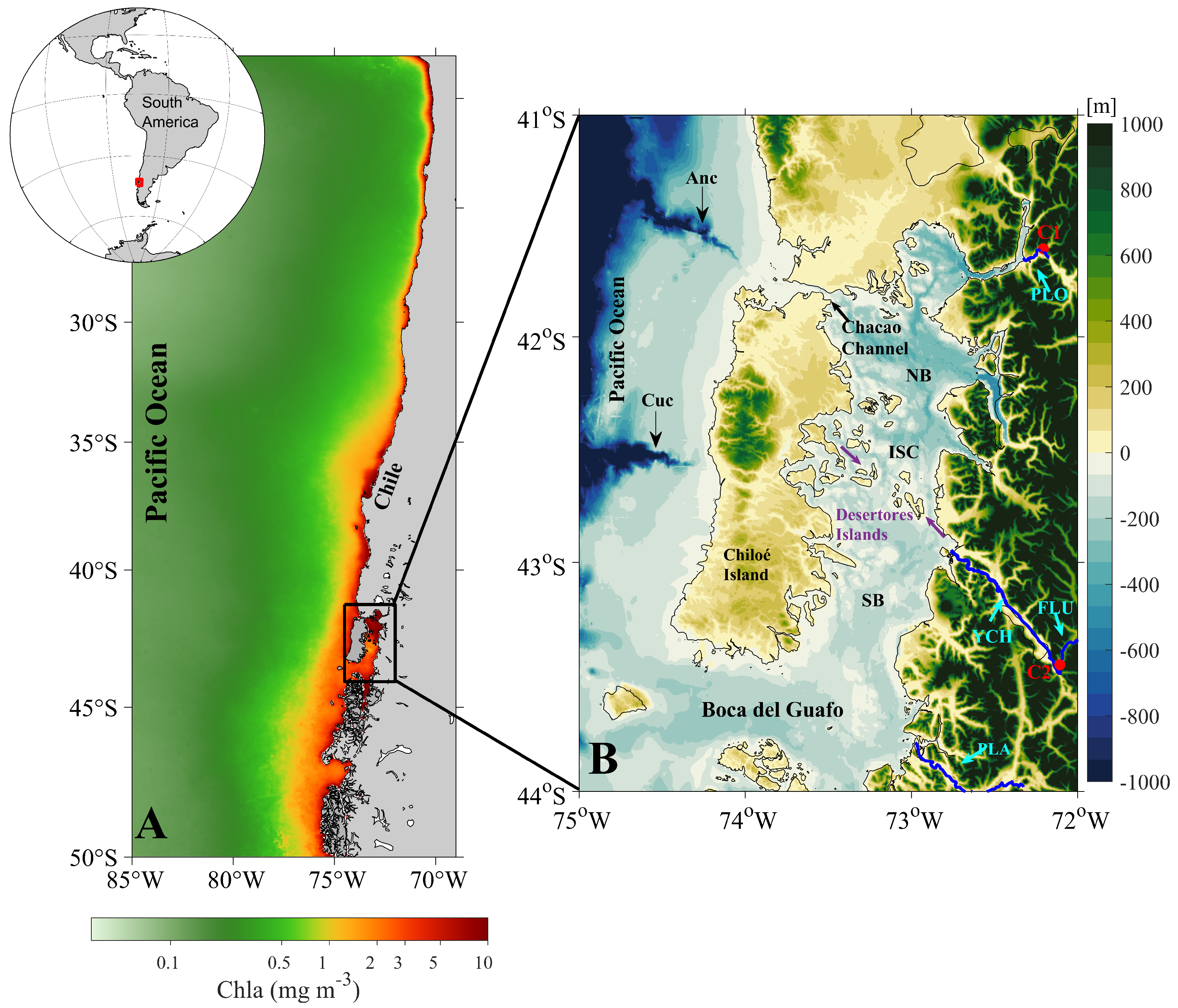
Abstract
:1. Introduction
2. Materials and Methods
2.1. Study Area
2.2. Satellite Data
2.3. River Discharge and Climatic Indices
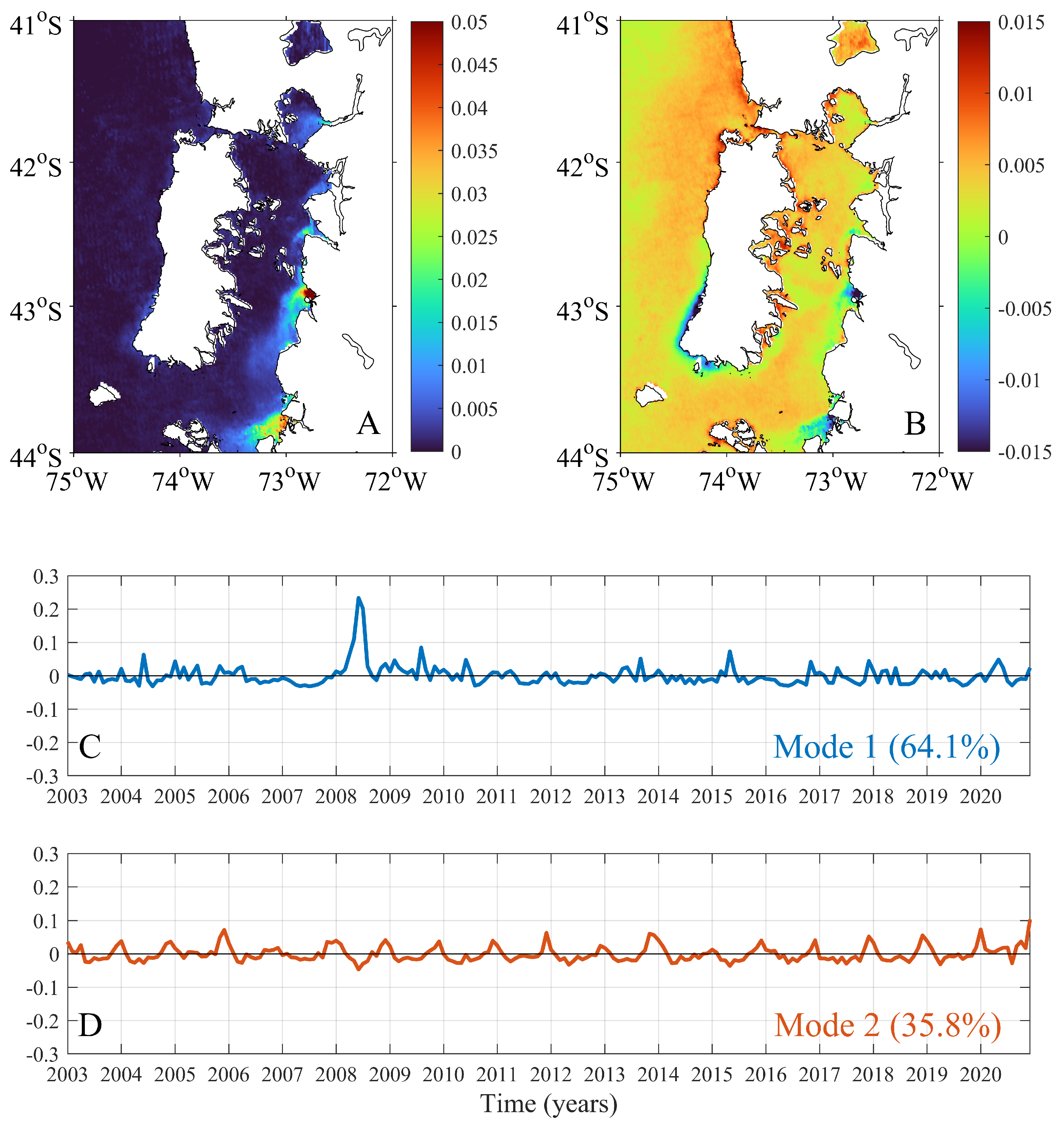
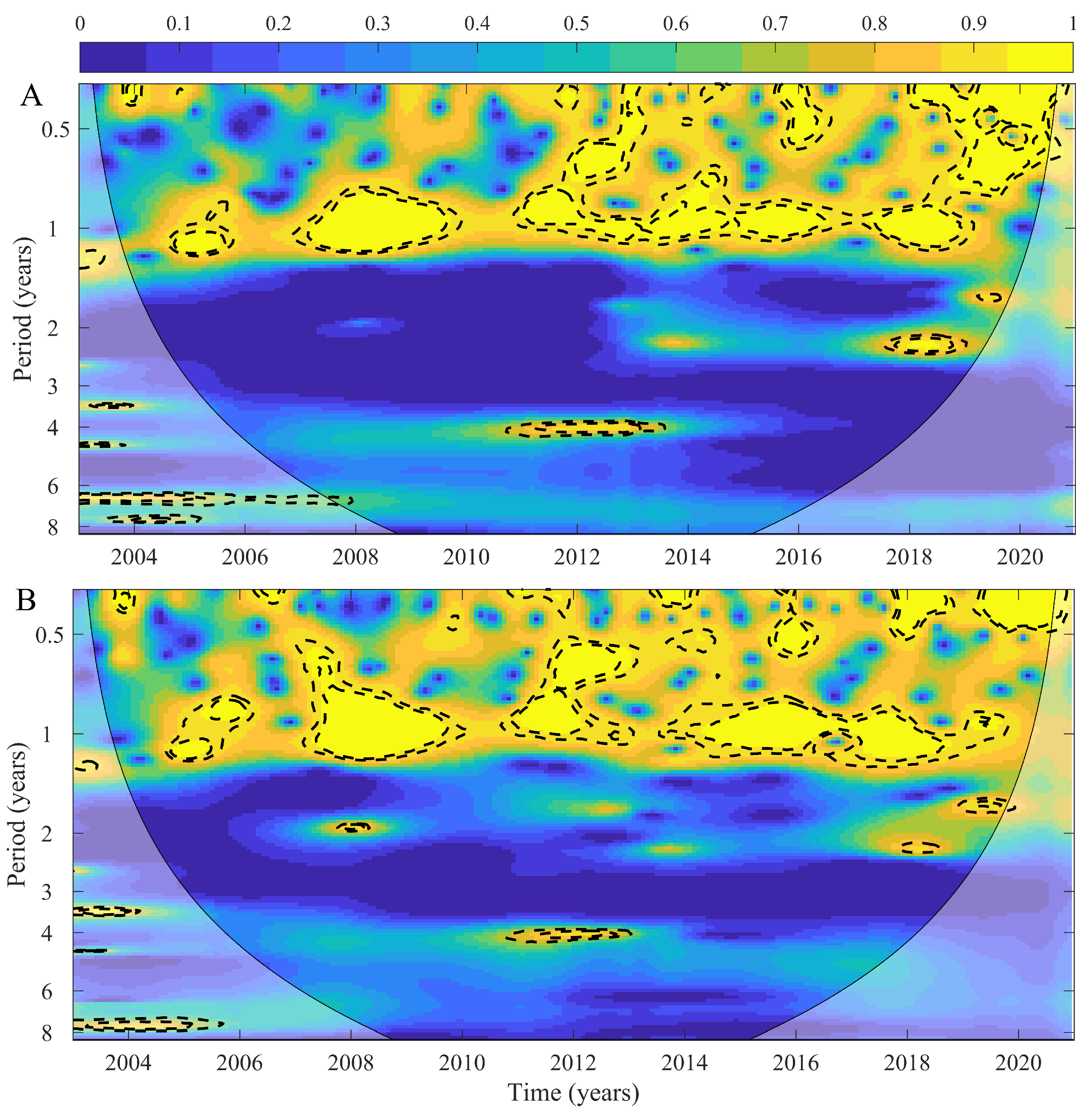
2.4. Wavelet and Temporal Synchrony in Northern Patagonia
3. Results
4. Discussion
5. Conclusions
Author Contributions
Funding
Data Availability Statement
Conflicts of Interest
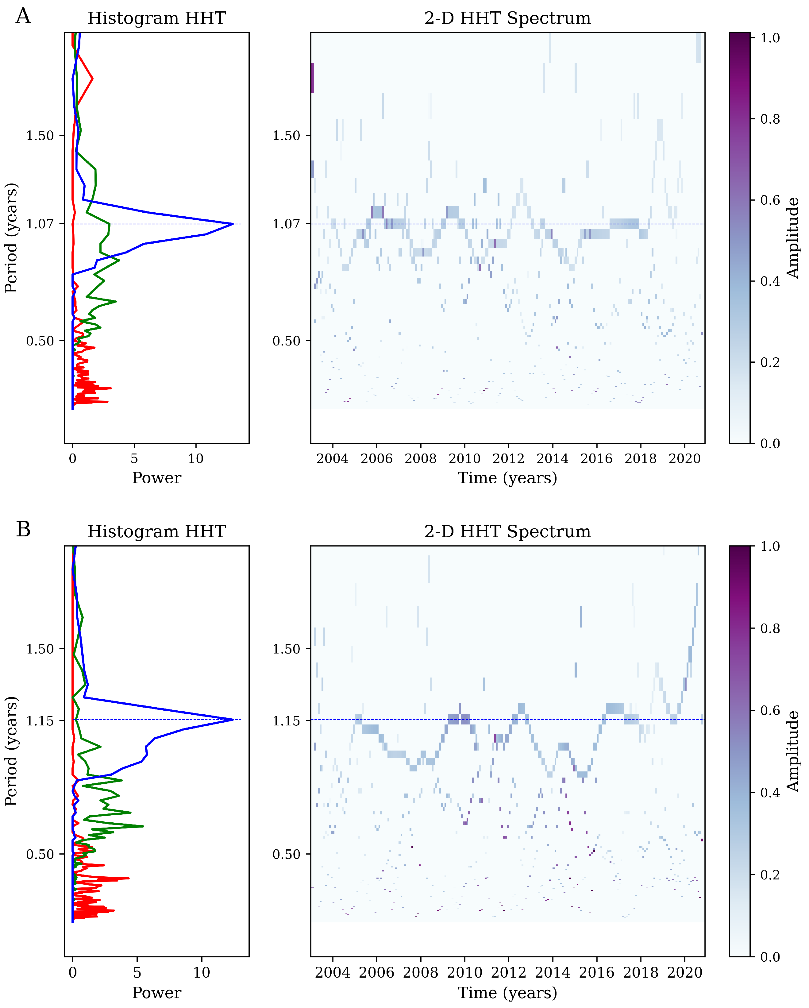
Appendix A. Hilbert–Huang Transform (HHT) Analysis


References
- Gouhier, T.C.; Guichard, F. Synchrony: Quantifying variability in space and time. Methods Ecol. Evol. 2014, 5, 524–533. [Google Scholar] [CrossRef]
- Chavez, M.; Cazelles, B. Detecting dynamic spatial correlation patterns with generalized wavelet coherence and non-stationary surrogate data. Sci. Rep. 2019, 9, 1–9. [Google Scholar] [CrossRef] [PubMed]
- Navarrete, S.S.A.S.; Broitman, B.R.; Menge, B.A.B. Interhemispheric comparison of recruitment to intertidal communities: Pattern persistence and scales of variation. Ecology 2008, 89, 1308–1322. [Google Scholar] [CrossRef]
- Koenig, W.D.; Liebhold, A.M. Temporally increasing spatial synchrony of North American temperature and bird populations. Nat. Clim. Chang. 2016, 6, 614–617. [Google Scholar] [CrossRef]
- Desharnais, R.A.; Reuman, D.C.; Costantino, R.F.; Cohen, J.E. Temporal scale of environmental correlations affects ecological synchrony. Ecol. Lett. 2018, 21, 1800–1811. [Google Scholar] [CrossRef] [PubMed]
- Anderson, T.L.; Sheppard, L.W.; Walter, J.A.; Hendricks, S.P.; Levine, T.D.; White, D.S.; Reuman, D.C. The dependence of synchrony on timescale and geography in freshwater plankton. Limnol. Oceanogr. 2019, 64, 483–502. [Google Scholar] [CrossRef]
- Defriez, E.J.; Reuman, D.C. A global geography of synchrony for marine phytoplankton. Glob. Ecol. Biogeogr. 2017, 26, 867–877. [Google Scholar] [CrossRef]
- Tanner, S.E.; Giacomello, E.; Menezes, G.M.; Mirasole, A.; Neves, J.; Sequeira, V.; Vasconcelos, R.P.; Vieira, A.R.; Morrongiello, J.R. Marine regime shifts impact synchrony of deep-sea fish growth in the northeast Atlantic. Oikos 2020, 129, 1781–1794. [Google Scholar] [CrossRef]
- Marshall, K.N.; Duffy-Anderson, J.T.; Ward, E.J.; Anderson, S.C.; Hunsicker, M.E.; Williams, B.C. Long-term trends in ichthyoplankton assemblage structure, biodiversity, and synchrony in the Gulf of Alaska and their relationships to climate. Prog. Oceanogr. 2019, 170, 134–145. [Google Scholar] [CrossRef]
- Hunt, G.L., Jr.; Coyle, K.O.; Eisner, L.B.; Farley, E.V.; Heintz, R.A.; Mueter, F.; Napp, J.M.; Overland, J.E.; Ressler, P.H.; Salo, S.; et al. Climate impacts on eastern Bering Sea foodwebs: A synthesis of new data and an assessment of the Oscillating Control Hypothesis. ICES J. Mar. Sci. 2011, 68, 1230–1243. [Google Scholar] [CrossRef]
- Batchelder, H.P.; Mackas, D.L.; O’Brien, T.D. Spatial–temporal scales of synchrony in marine zooplankton biomass and abundance patterns: A world-wide comparison. Prog. Oceanogr. 2012, 97, 15–30. [Google Scholar] [CrossRef]
- Ong, J.J.; Rountrey, A.N.; Zinke, J.; Meeuwig, J.J.; Grierson, P.F.; O’Donnell, A.J.; Newman, S.J.; Lough, J.M.; Trougan, M.; Meekan, M.G. Evidence for climate-driven synchrony of marine and terrestrial ecosystems in northwest Australia. Glob. Chang. Biol. 2016, 22, 2776–2786. [Google Scholar] [CrossRef] [PubMed]
- Defriez, E.J.; Sheppard, L.W.; Reid, P.C.; Reuman, D.C. Climate change-related regime shifts have altered spatial synchrony of plankton dynamics in the North Sea. Glob. Chang. Biol. 2016, 22, 2069–2080. [Google Scholar] [CrossRef] [PubMed]
- Messié, M.; Chavez, F.P. A global analysis of ENSO synchrony: The oceans’ biological response to physical forcing. J. Geophys. Res. Ocean. 2012, 117, C09001. [Google Scholar] [CrossRef]
- He, J.; Christakos, G.; Cazelles, B.; Wu, J.; Leng, J. Spatio–temporal variation of the association between sea surface temperature and chlorophyll in global ocean during 2002–2019 based on a novel WCA-BME approach. Int. J. Appl. Earth Obs. Geoinf. 2021, 105, 102620. [Google Scholar]
- da Silva, M.N.; Granzotti, R.V.; de Carvalho, P.; Rodrigues, L.C.; Bini, L.M. Niche measures and growth rate do not predict interspecific variation in spatial synchrony of phytoplankton. Limnology 2021, 22, 121–127. [Google Scholar] [CrossRef]
- Cazelles, B.; Chavez, M.; Berteaux, D.; Ménard, F.; Vik, J.O.; Jenouvrier, S.; Stenseth, N.C. Wavelet analysis of ecological time series. Oecologia 2008, 156, 287–304. [Google Scholar] [CrossRef]
- Roushangar, K.; Alizadeh, F.; Adamowski, J. Exploring the effects of climatic variables on monthly precipitation variation using a continuous wavelet-based multiscale entropy approach. Environ. Res. 2018, 165, 176–192. [Google Scholar] [CrossRef]
- Xiao, X.; He, J.; Yu, Y.; Cazelles, B.; Li, M.; Jiang, Q.; Xu, C. Teleconnection between phytoplankton dynamics in north temperate lakes and global climatic oscillation by time-frequency analysis. Water Res. 2019, 154, 267–276. [Google Scholar] [CrossRef]
- Yadav, J.; Kumar, A.; Srivastava, A.; Mohan, R. Sea ice variability and trends in the Indian Ocean sector of Antarctica: Interaction with ENSO and SAM. Environ. Res. 2022, 212, 113481. [Google Scholar] [CrossRef]
- Ménard, F.; Marsac, F.; Bellier, E.; Cazelles, B. Climatic oscillations and tuna catch rates in the Indian Ocean: A wavelet approach to time series analysis. Fish. Oceanogr. 2007, 16, 95–104. [Google Scholar] [CrossRef]
- Buttay, L.; Cazelles, B.; Miranda, A.; Casas, G.; Nogueira, E.; González-Quirós, R. Environmental multi-scale effects on zooplankton inter-specific synchrony. Limnol. Oceanogr. 2017, 62, 1355–1365. [Google Scholar] [CrossRef]
- León-Muñoz, J.; Urbina, M.A.; Garreaud, R.; Iriarte, J.L. Hydroclimatic conditions trigger record harmful algal bloom in western Patagonia (summer 2016). Sci. Rep. 2018, 8, 1–10. [Google Scholar] [CrossRef] [PubMed]
- Curra-Sánchez, E.D.; Lara, C.; Cornejo-D’Ottone, M.; Nimptsch, J.; Aguayo, M.; Broitman, B.R.; Saldías, G.S.; Vargas, C.A. Contrasting land-uses in two small river basins impact the colored dissolved organic matter concentration and carbonate system along a river-coastal ocean continuum. Sci. Total Environ. 2022, 806, 150435. [Google Scholar] [CrossRef]
- González, H.; Calderón, M.; Castro, L.; Clement, A.; Cuevas, L.; Daneri, G.; Iriarte, J.; Lizárraga, L.; Martínez, R.; Menschel, E.; et al. Primary production and plankton dynamics in the Reloncaví Fjord and the Interior Sea of Chiloé, Northern Patagonia, Chile. Mar. Ecol. Prog. Ser. 2010, 402, 13–30. [Google Scholar] [CrossRef]
- Cuevas, L.A.; Tapia, F.J.; Iriarte, J.L.; González, H.E.; Silva, N.; Vargas, C.A. Interplay between freshwater discharge and oceanic waters modulates phytoplankton size-structure in fjords and channel systems of the Chilean Patagonia. Prog. Oceanogr. 2019, 173, 103–113. [Google Scholar] [CrossRef]
- Galán, A.; Saldías, G.S.; Corredor-Acosta, A.; Muñoz, R.; Lara, C.; Iriarte, J.L. Argo float reveals biogeochemical characteristics along the freshwater gradient off western Patagonia. Front. Mar. Sci. 2021, 8, 613265. [Google Scholar] [CrossRef]
- Lara, C.; Cazelles, B.; Saldías, G.S.; Flores, R.P.; Paredes, Á.L.; Broitman, B.R. Coupled biospheric synchrony of the coastal temperate ecosystem in Northern Patagonia: A remote sensing analysis. Remote Sens. 2019, 11, 2092. [Google Scholar] [CrossRef]
- Strub, P.T.; James, C.; Montecino, V.; Rutllant, J.A.; Blanco, J.L. Ocean circulation along the southern Chile transition region (38–46 S): Mean, seasonal and interannual variability, with a focus on 2014–2016. Prog. Oceanogr. 2019, 172, 159–198. [Google Scholar] [CrossRef]
- Thomas, A.C.; Brickley, P.; Weatherbee, R. Interannual variability in chlorophyll concentrations in the Humboldt and California Current Systems. Prog. Oceanogr. 2009, 83, 386–392. [Google Scholar] [CrossRef]
- Fogt, R.L.; Marshall, G.J. The Southern Annular Mode: Variability, trends, and climate impacts across the Southern Hemisphere. Wiley Interdiscip. Rev. Clim. Chang. 2020, 11, e652. [Google Scholar] [CrossRef]
- Giesecke, R.; Clement, A.; Garcés-Vargas, J.; Mardones, J.I.; González, H.E.; Caputo, L.; Castro, L. Massive salp outbreaks in the Inner Sea of Chiloé Island (Southern Chile): Possible causes and ecological consequences. Lat. Am. J. Aquat. Res. 2014, 42, 604–621. [Google Scholar] [CrossRef]
- Lara, C.; Saldías, G.S.; Tapia, F.J.; Iriarte, J.L.; Broitman, B.R. Interannual variability in temporal patterns of Chlorophyll–a and their potential influence on the supply of mussel larvae to inner waters in northern Patagonia (41°–44°S). J. Mar. Syst. 2016, 155, 11–18. [Google Scholar] [CrossRef]
- Saldías, G.S.; Hernández, W.; Lara, C.; Muñoz, R.; Rojas, C.; Vásquez, S.; Pérez-Santos, I.; Soto-Mardones, L. Seasonal variability of SST fronts in the Inner Sea of Chiloé and its adjacent coastal ocean, northern Patagonia. Remote Sens. 2021, 13, 181. [Google Scholar] [CrossRef]
- FAO. State of the World Fisheries and Aquaculture—2022 (SOFIA); FAO: Rome, Italy, 2022; p. 236. [Google Scholar]
- SERNAPESCA, Servicio Nacional de Pesca y Acuicultura. Anuario Estadístico de Pesca; Ministerio de Economía: Fomento y Turismo, Chile, 2022.
- Narváez, D.A.; Vargas, C.A.; Cuevas, L.A.; García-Loyola, S.A.; Lara, C.; Segura, C.; Tapia, F.J.; Broitman, B.R. Dominant scales of subtidal variability in coastal hydrography of the Northern Chilean Patagonia. J. Mar. Syst. 2019, 193, 59–73. [Google Scholar] [CrossRef]
- Vásquez, S.I.; de la Torre, M.B.; Saldías, G.S.; Montecinos, A. Meridional Changes in Satellite Chlorophyll and Fluorescence in Optically-Complex Coastal Waters of Northern Patagonia. Remote Sens. 2021, 13, 1026. [Google Scholar] [CrossRef]
- Flores, R.P.; Lara, C.; Saldías, G.S.; Vásquez, S.I.; Roco, A. Spatio-temporal variability of turbid freshwater plumes in the Inner Sea of Chiloé, northern Patagonia. J. Mar. Syst. 2022, 228, 103709. [Google Scholar] [CrossRef]
- Saldías, G.S.; Sobarzo, M.; Quiñones, R. Freshwater structure and its seasonal variability off western Patagonia. Prog. Oceanogr. 2019, 174, 143–153. [Google Scholar] [CrossRef]
- Lara, C.; Miranda, M.; Montecino, V.; Iriarte, J.L. Chlorophyll-a MODIS mesoscale variability in the Inner Sea of Chiloé, Patagonia, Chile (41-43°S): Patches and Gradients? Rev. De Biol. Mar. Y Oceanogr. 2010, 45, 217–225. [Google Scholar] [CrossRef]
- O’Reilly, J.E.; Maritorena, S.; Siegel, D.A.; O’Brien, M.C.; Toole, D.; Mitchell, B.G.; Kahru, M.; Chavez, F.P.; Strutton, P.; Cota, G.F.; et al. Ocean color chlorophyll a algorithms for SeaWiFS, OC2, and OC4: Version 4. SeaWiFS Postlaunch Calibration Valid. Anal. Part 2000, 3, 9–23. [Google Scholar]
- Garreaud, R. Record-breaking climate anomalies lead to severe drought and environmental disruption in western Patagonia in 2016. Clim. Res. 2018, 74, 217–229. [Google Scholar] [CrossRef]
- Thomson, R.E.; Emery, W.J. Data Analysis Methods in Physical Oceanography; Newnes: Boston, MA, USA, 2014. [Google Scholar]
- Cazelles, B.; Chavez, M.; Magny, G.C.d.; Guégan, J.F.; Hales, S. Time-dependent spectral analysis of epidemiological time-series with wavelets. J. R. Soc. Interface 2007, 4, 625–636. [Google Scholar] [CrossRef] [PubMed]
- Medkour, T.; Walden, A.T.; Burgess, A. Graphical modelling for brain connectivity via partial coherence. J. Neurosci. Meth. 2009, 180, 374–383. [Google Scholar] [CrossRef]
- Cazelles, B.; Chavez, M.; McMichael, A.J.; Hales, S. Nonstationary influence of El Nino on the synchronous dengue epidemics in Thailand. PLoS Med. 2005, 2, e106. [Google Scholar] [CrossRef] [PubMed]
- Huang, N.E.; Shen, Z.; Long, S.R.; Wu, M.C.; Shih, H.H.; Zheng, Q.; Yen, N.C.; Tung, C.C.; Liu, H.H. The empirical mode decomposition and the Hilbert spectrum for nonlinear and non-stationary time series analysis. Proc. R. Soc. London Ser. A Math. Phys. Eng. Sci. 1998, 454, 903–995. [Google Scholar] [CrossRef]
- Huang, N.E.; Wu, M.L.C.; Long, S.R.; Shen, S.S.; Qu, W.; Gloersen, P.; Fan, K.L. A confidence limit for the empirical mode decomposition and Hilbert spectral analysis. Proc. R. Soc. London Ser. A Math. Phys. Eng. Sci. 2003, 459, 2317–2345. [Google Scholar] [CrossRef]
- Cazelles, B.; Cazelles, K.; Chavez, M. Wavelet analysis in ecology and epidemiology: Impact of statistical tests. J. R. Soc. Interface 2014, 11, 20130585. [Google Scholar] [CrossRef]
- He, J.; Christakos, G.; Zhang, W.; Wang, Y. A space-time study of hemorrhagic fever with renal syndrome (HFRS) and its climatic associations inHeilongjiang province, China. Front. Appl. Math. Stat. 2017, 3, 16. [Google Scholar] [CrossRef]
- He, J.; Christakos, G.; Wu, J.; Cazelles, B.; Qian, Q.; Mu, D.; Wang, Y.; Yin, W.; Zhang, W. Spatiotemporal variation of the association between climate dynamics and HFRS outbreaks in Eastern China during 2005-2016 and its geographic determinants. PLoS Neglected Trop. Dis. 2018, 12, e0006554. [Google Scholar] [CrossRef]
- Xiao, X.; He, J.; Huang, H.; Miller, T.R.; Christakos, G.; Reichwaldt, E.S.; Ghadouani, A.; Lin, S.; Xu, X.; Shi, J. A novel single-parameter approach for forecasting algal blooms. Water Res. 2017, 108, 222–231. [Google Scholar] [CrossRef]
- Kowalczuk, P. Seasonal variability of yellow substance absorption in the surface layer of the Baltic Sea. J. Geophys. Res. Ocean. 1999, 104, 30047–30058. [Google Scholar] [CrossRef]
- Darecki, M.; Weeks, A.; Sagan, S.; Kowalczuk, P.; Kaczmarek, S. Optical characteristics of two contrasting Case 2 waters and their influence on remote sensing algorithms. Cont. Shelf Res. 2003, 23, 237–250. [Google Scholar] [CrossRef]
- Mishra, S.; Mishra, D.R. Normalized Difference Chlorophyll Index: A novel model for remote estimation of chlorophyll-a concentration in turbid productive waters. Remote Sens. Environ. 2012, 117, 394–406. [Google Scholar] [CrossRef]
- D’Sa, E.J.; Miller, R.L. Bio-optical properties in waters influenced by the Mississippi River during low flow conditions. Remote Sens. Environ. 2003, 84, 538–549. [Google Scholar] [CrossRef]
- Hestir, E.L.; Brando, V.E.; Bresciani, M.; Giardino, C.; Matta, E.; Villa, P.; Dekker, A.G. Measuring freshwater aquatic ecosystems: The need for a hyperspectral global mapping satellite mission. Remote Sens. Environ. 2015, 167, 181–195. [Google Scholar] [CrossRef]
- Dávila, P.M.; Figueroa, D.; Müller, E. Freshwater input into the coastal ocean and its relation with the salinity distribution off austral Chile (35–55°S). Cont. Shelf Res. 2002, 22, 521–534. [Google Scholar] [CrossRef]
- Wu, Z.; Huang, N.E.; Long, S.R.; Peng, C.K. On the trend, detrending, and variability of nonlinear and nonstationary time series. Proc. Natl. Acad. Sci. USA 2007, 104, 14889–14894. [Google Scholar] [CrossRef]
- Aguayo, R.; León-Muñoz, J.; Garreaud, R.; Montecinos, A. Hydrological droughts in the southern Andes (40–45°S) from an ensemble experiment using CMIP5 and CMIP6 models. Sci. Rep. 2021, 11, 1–16. [Google Scholar] [CrossRef]
- Garreaud, R.D.; Alvarez-Garreton, C.; Barichivich, J.; Boisier, J.P.; Christie, D.; Galleguillos, M.; LeQuesne, C.; McPhee, J.; Zambrano-Bigiarini, M. The 2010–2015 megadrought in central Chile: Impacts on regional hydroclimate and vegetation. Hydrol. Earth Syst. Sci. 2017, 21, 6307–6327. [Google Scholar] [CrossRef]
- Lara, C.; Saldías, G.S.; Cazelles, B.; Rivadeneira, M.M.; Haye, P.A.; Broitman, B.R. Coastal biophysical processes and the biogeography of rocky intertidal species along the south-eastern Pacific. J. Biogeogr. 2019, 46, 420–431. [Google Scholar] [CrossRef]
- Crawford, D.W.; Montero, P.; Daneri, G. Blooms of Alexandrium catenella in Coastal Waters of Chilean Patagonia: Is Subantarctic Surface Water Involved? Front. Mar. Sci. 2021, 8, 612628. [Google Scholar] [CrossRef]
- Díaz, P.A.; Peréz-Santos, I.; Álvarez, G.; Garreaud, R.; Pinilla, E.; Díaz, M.; Sandoval, A.; Araya, M.; Álvarez, F.; Rengel, J.; et al. Multiscale physical background to an exceptional harmful algal bloom of Dinophysis acuta in a fjord system. Sci. Total Environ. 2021, 773, 145621. [Google Scholar] [CrossRef] [PubMed]
- Aguayo, R.; León-Muñoz, J.; Vargas-Baecheler, J.; Montecinos, A.; Garreaud, R.; Urbina, M.; Soto, D.; Iriarte, J.L. The glass half-empty: Climate change drives lower freshwater input in the coastal system of the Chilean Northern Patagonia. Clim. Chang. 2019, 155, 417–435. [Google Scholar] [CrossRef]
- Hansen, B.B.; Grøtan, V.; Herfindal, I.; Lee, A.M. The Moran effect revisited: Spatial population synchrony under global warming. Ecography 2020, 43, 1591–1602. [Google Scholar] [CrossRef]
- Cavanaugh, K.C.; Kendall, B.E.; Siegel, D.A.; Reed, D.C.; Alberto, F.; Assis, J. Synchrony in dynamics of giant kelp forests is driven by both local recruitment and regional environmental controls. Ecology 2013, 94, 499–509. [Google Scholar] [CrossRef]
- Mandal, S.; Nair, M.A.; Kumar, V.S. Hilbert-Huang transform analysis of surface wavefield under tropical cyclone Hudhud. Appl. Ocean Res. 2020, 101, 102269. [Google Scholar] [CrossRef]
- Quinn, A.J.; Lopes-dos Santos, V.; Dupret, D.; Nobre, A.C.; Woolrich, M.W. EMD: Empirical mode decomposition and Hilbert-Huang spectral analyses in Python. J. Open Source Softw. 2021, 6, 2977. [Google Scholar] [CrossRef]


Disclaimer/Publisher’s Note: The statements, opinions and data contained in all publications are solely those of the individual author(s) and contributor(s) and not of MDPI and/or the editor(s). MDPI and/or the editor(s) disclaim responsibility for any injury to people or property resulting from any ideas, methods, instructions or products referred to in the content. |
© 2023 by the authors. Licensee MDPI, Basel, Switzerland. This article is an open access article distributed under the terms and conditions of the Creative Commons Attribution (CC BY) license (https://creativecommons.org/licenses/by/4.0/).
Share and Cite
Muñoz, R.; Lara, C.; Arteaga, J.; Vásquez, S.I.; Saldías, G.S.; Flores, R.P.; He, J.; Broitman, B.R.; Cazelles, B. Temporal Synchrony in Satellite-Derived Ocean Parameters in the Inner Sea of Chiloé, Northern Patagonia, Chile. Remote Sens. 2023, 15, 2182. https://doi.org/10.3390/rs15082182
Muñoz R, Lara C, Arteaga J, Vásquez SI, Saldías GS, Flores RP, He J, Broitman BR, Cazelles B. Temporal Synchrony in Satellite-Derived Ocean Parameters in the Inner Sea of Chiloé, Northern Patagonia, Chile. Remote Sensing. 2023; 15(8):2182. https://doi.org/10.3390/rs15082182
Chicago/Turabian StyleMuñoz, Richard, Carlos Lara, Johny Arteaga, Sebastián I. Vásquez, Gonzalo S. Saldías, Raúl P. Flores, Junyu He, Bernardo R. Broitman, and Bernard Cazelles. 2023. "Temporal Synchrony in Satellite-Derived Ocean Parameters in the Inner Sea of Chiloé, Northern Patagonia, Chile" Remote Sensing 15, no. 8: 2182. https://doi.org/10.3390/rs15082182