1. Introduction
Since the first remote sensing (RS) satellite termed Sputnik-1 was launched in 1957, the collection of RS images from space has been uninterrupted [
1]. The imaging mode of visible RS images is most consistent with human visual perception. This characteristic has led to the development of several ground detection techniques and continuous monitoring methods. In addition, it has found considerable applications in disaster relief, geology, environmental monitoring, and engineering construction, accompanied by extensive promotion and adoption [
2]. Nonetheless, the global surface cloud coverage can fluctuate between 58% [
3] and 61% [
4], which, subsequently, leads to a reduction in the availability of most visible remote sensing products.
Therefore, enhancing the efficacy of visible RS images is of utmost importance. Furthermore, the process of cloud removal can be regarded as a type of image reconstruction, which is heavily dependent on precise cloud detection [
5]. The principal techniques for cloud removal can be divided into two primary categories based on the number of RS images utilized: multi-temporal methods and single-image methods [
6,
7,
8,
9].
Cloud removal in time-series remote sensing images is a widely used method, particularly in big data platforms such as the Google Earth Engine, which involves combining same-track images for efficient image element replacement. Researchers have established various cloud removal restoration models, such as those using dictionary learning [
10,
11], spatially and temporally weighted regression [
12], low-rank representation [
13], deep learning [
9,
14], and nonnegative matrix factorization [
15]. Despite this, removing time-series remote sensing images may result in inconsistent image tone and surface information due to the temporal consistency and seasonal variability of remote sensing images, especially in tropical and mountainous regions, where the number of cloud-free images is limited, further exacerbating information variability.
Single remote sensing image cloud removal can be achieved using four primary methods: image enhancement, spatial interpolation, atmospheric transport model, and generate adversarial network-based surface information reconstruction. Image enhancement methods alter contrast and weaken image components to suppress clouds, resulting in unrealistic visual completion that cannot be used for remote sensing target detection and quantitative analysis [
16,
17,
18]. Spatial interpolation techniques such as Kriging spatial interpolation and the neighborhood similar pixel interpolator can eliminate speckled clouds, but they face challenges in effectively recovering the surface information under a wide range of clouds [
19,
20,
21]. Atmospheric transport models such as haze-optimized transformation and dark channel defogging exploit prior knowledge and can effectively remove clouds, but changes in the prior knowledge may lead to biased image estimates [
7,
8,
22,
23]. Generative adversarial networks have shown promise in cloud removal and surface information reconstruction, but they do not recognize when thin and thick clouds coexist, resulting in significant disparities between the output and original image [
24,
25,
26,
27,
28].
Recently, researchers have proposed novel techniques for improving the stability of remote sensing images through cloud removal. Li et al. developed a deep-learning-based approach, CR-MSS, which leverages short-wave infrared to eliminate thin clouds from high-resolution images [
29]. Image matting technology has also made significant advances in recent years [
30,
31,
32,
33,
34], finding applications in fields such as image fusion [
35], shadow removal [
36], semantic segmentation [
37], image defogging [
38], cloud estimation [
39], and beyond. By overlaying foreground and background images and measuring foreground transparency, precise foreground information can be extracted.
CNNs are highly competent in extracting image features as a result of their local connectivity, parameter sharing, and translational invariance, resulting in a more comprehensive feature extraction compared to generative adversarial networks [
40]. Moreover, CNN optimization is simpler, and the model quickly and stably converges. In this study, our primary goal is to estimate cloud opacity, which may be considered a type of noise (akin to Perlin noise). While the discriminator can create a more natural, smooth, and visually appealing generated image in generative adversarial networks, the generator can easily generate noise signals to deceive the discriminator, which may result in limited significance of the loss function presented by the discriminator and instability in the model training process. Thus, we suggest employing a CNN to assess the background information and extract the foreground information in the image. Based on this, we propose the “SCM-CNN” (Saliency Cloud Matting Convolutional Neural Network) model that integrates deep learning techniques with image matting for remote sensing image cloud recognition, cloud opacity estimation, and cloud removal.
The conventional method for image matting necessitates the incorporation of a “Trimap”, which involves the triple classification of images. To lessen the model’s dependence on Trimaps, we employed a saliency monitoring network to enhance the model’s applicability.
It is crucial to acknowledge that the surface characteristics will evolve over time, and the levels of solar radiation and aerosol concentration will vary with each RS satellite observation. Obtaining an actual control group of overcast and clear images is unfeasible. Therefore, creating an RS image that is as close to reality as possible is a prerequisite for the SCM-CNN model to converge successfully. In this regard, we refer to Matting dataset construction scenarios such as the alpha-matting dataset [
41], the portrait image matting dataset [
42], and the traditional RS image process for generating samples for cloud detection, such as L7 Irish [
43] and L8 SPARCS [
44], in this study. Cloud opacity is determined based on the color range extracted from Sentinel-2 satellite images covering the sea’s surface. Subsequently, the samples are aggregated into a single image to form the precise label, and then the training and validation dataset required for the study are constructed using the RGB band images of cloud-free Sentinel-2 as the base image.
The contributions of this article are summarized as follows.
We constructed a cloud-matting dataset generation method and created a set of high-quality cloud-matting datasets based on Sentinel-2 imagery. The cloud-matting dataset outperforms the commonly used semantic labels for cloud detection, by effectively distinguishing the clouded and cloud-free areas in RS images with 100% accuracy. Moreover, it accurately describes the mixing degree of image elements in cloud-covered areas. As the cloud-matting dataset closely resembles cloud scenes in real RS images, it enables various applications such as accurate cloud detection, image reconstruction, and cloud opacity estimation.
This work presents an integrated model for cloud detection, cloud opacity estimation, and cloud removal based on the principle of deep learning Image-matting. The model utilizes the saliency detection function to eliminate the need for a “Trimap”, enabling cloud removal from a different perspective. Cloud removal in this model relies on cloud identification and similarity analysis with the original image. It effectively recovers the surface area beneath thin clouds, even in scenarios of coexisting thick and thin clouds.
The proposed method includes a “Channel Global Max/Average Pooling” structure that estimates the reflection of the foreground pixel efficiently with minimal parameters. The structure efficiently extracts the foreground pixel reflection with minimal parameters from the feature map.
Our proposed method is a multi-objective loss function gradient optimization approach that calculates the gradient deviation of the loss function rather than relying on the conventional weight linear combination of multiple loss functions. The model gradient is updated accordingly.
The following is the organization of this article.
Section 2 presents the superposition model of the remote sensing (RS) images, the formulation of cloud removal under the image matting framework, and the dataset and evaluation metrics that were utilized.
Section 3 provides a detailed exposition of the experimental procedures and results. In
Section 4, we analyze the relative advantages and disadvantages of various methods and propose possible enhancements. Finally,
Section 5 draws conclusive remarks.
2. Materials and Methods
2.1. Dataset
The current cloud dataset is primarily designed for cloud detection, using a mask to distinguish cloud areas from others. However, this dataset is unsuitable for cloud–fog retrieval tasks, and its inherent bias may significantly reduce the accuracy of machine learning models. To address these issues, we employ a colorimetric approach and Sentinel-2 satellite ocean imagery to obtain simulated cloud images and establish a normalized cloud opacity layer. By overlaying and merging opacity layers of cloud layers from multiple scenes, we were able to generate highly realistic cloud simulations.
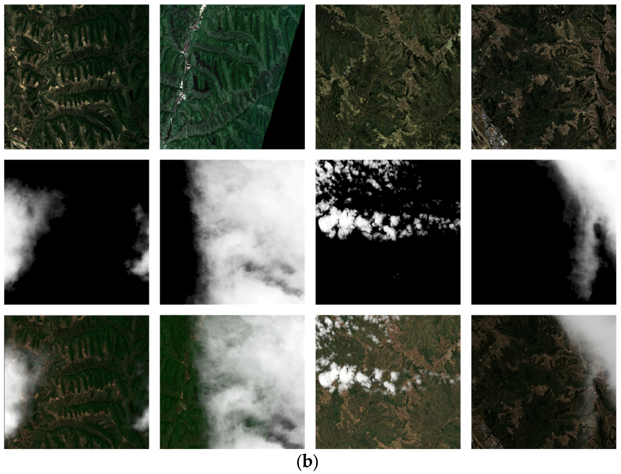
Cloud-Free Image Construction: Our objective was to remove thin clouds under less cloudy mountainous conditions. To achieve this, we used a dataset of 24 Sentinel-2 remote sensing images covering the southeastern Tibetan region. The images were processed with S2Cloudless to detect clouds and calculate cloud shadows based on satellite incidence angles and surface dark pixel information. A sliding window of a 512 × 512 pixel size with a step of 256 pixels was then used to traverse the images, generating cut-out remote sensing images without clouds and cloud shadows and discarding those with clouds or cloud shadows.
Cloud Opacity Image Construction: Some researchers utilized manual masking [
9] or Perlin noise [
45] to generate cloud images, while simulating cloud images that approximated real cloud distributions. Therefore, we extracted cloud distributions from actual ocean surface remote sensing images to simplify the process and reduce errors. Multiple Sentinel-2 remote sensing images were selected, and the opacity of clouds was extracted using a color range. The opacity of clouds was normalized, and image closing operations were performed to eliminate holes caused by convective cloud shadows. Multiple cloud opacity images with different cloud thicknesses and shapes were obtained by multiple extractions and merging.
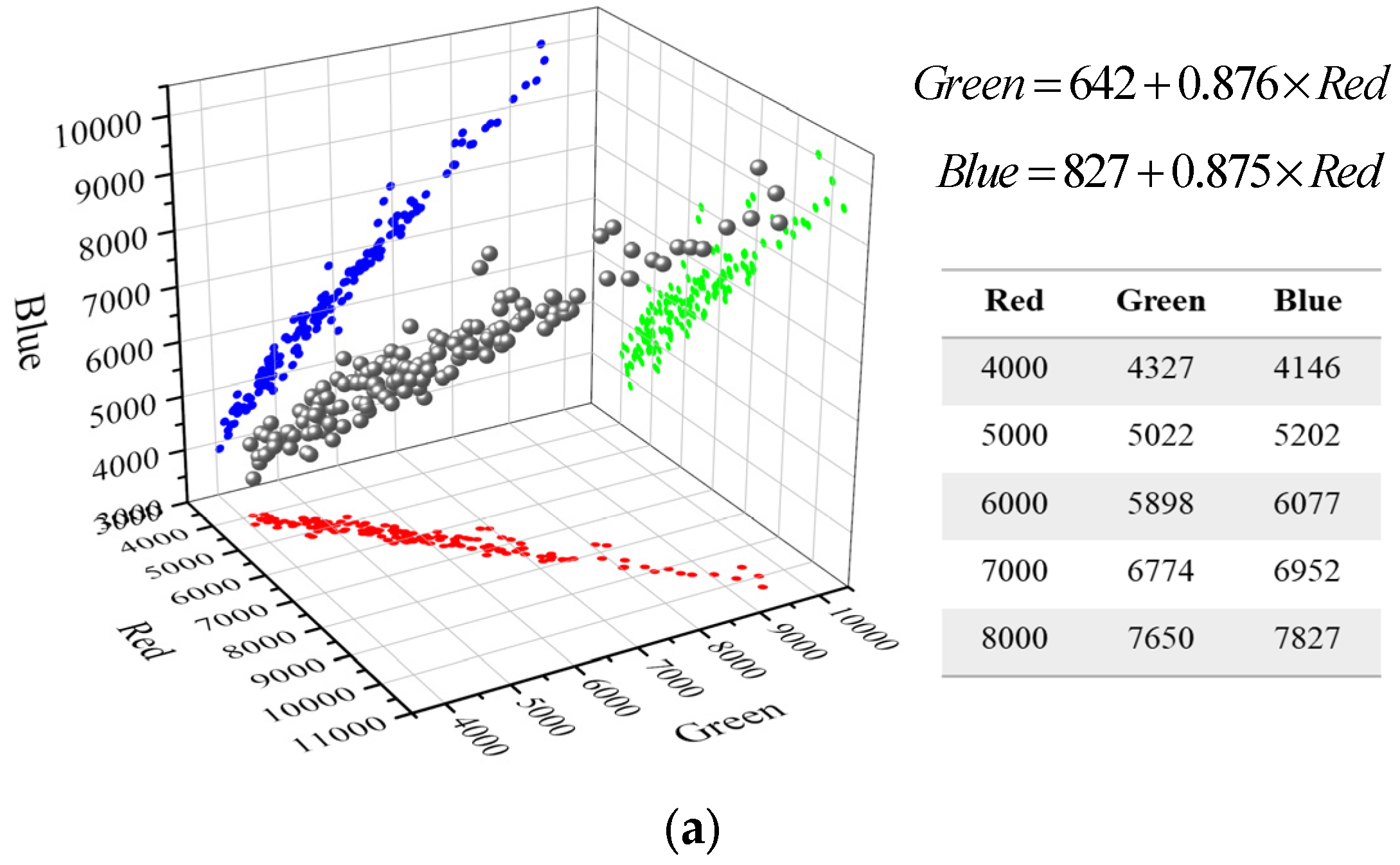
Simulating Cloud Image Generation: In Sentinel-2 images, there is no evident distinction between the red, green, and blue bands of cloud areas. They exhibit a strong linear relationship with some perturbations around the linear regression function. In
Figure 1a, we randomly selected some points for fitting, and the results indicated that there was little difference in pixel brightness between the red, green, and blue bands in the range of 4000–8000 pixels. As red, green, and blue all belong to the visible light band, their wavelengths vary slightly, resulting in similar penetration capabilities for clouds. Therefore, pixel value perturbations are more likely caused by factors such as surface objects, particles in the cloud layer, and aerosols. Simulating these perturbations is a complex task. To avoid human errors and simplify the model, we assume that the RGB bands of cloud layers in RS images have the same opacity value. According to the assumption in
Section 2.2 that
can be a constant in a local area, we simulated cloud images based on reference formula
, where
and
are 512 × 512 random blocks in the opacity map of cloud layers, as shown in
Figure 1b.
2.2. Superposition Model of RS Images
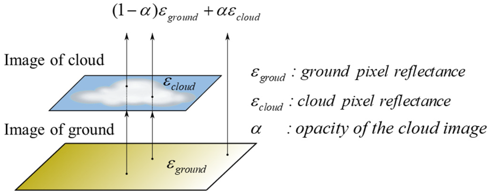
In
Figure 2, the cloud represents the foreground image, while the surface object acts as the background image, with the cloud’s opacity being corresponding to the foreground image’s opacity (
). As a result, the satellite RS image is formed after superimposing the background pixel reflection signal (
) and the foreground pixel reflection signal (
). The thin cloud effect is created by combining the multiplicative factor that attenuates the light from below the clouds and the additive factor that adds reflected light at the cloud tops.
This paper adopts image matting for RS image cloud removal, and the cloud shadow is not considered for the time being. If assuming that cloud shadow does not exist, Equation (1) is a simplified model which has three unknowns. Substantially, we only need to obtain the
and
to calculate
.
Nevertheless, it should be noted that
is independent of
if we use
to solve the derivative at both ends of Equation (2).
Equation (3) shows the relationship between and after each cloud removal restoration process in the image. When , the denominator is infinitely close to 0, and even a small perturbation will lead to a significant error, reducing the model’s reliability. For that reason, we classify clouds into thin clouds () and thick clouds (), according to their opacity.
2.3. Overview of SCM-CNN
The SCM-CNN model suggested in this research performs three significant roles, which are as follows.
I. Cloud matting: The central focus of the research presented in this paper is the concept of cloud matting, which ultimately leads to cloud opacity. In order to reduce model complexity, we have discontinued the use of the “Trimap” input and “Trimap” generating strategy, although this decision has resulted in significant challenges for model inference. To address this issue, we propose the use of a salient target detection function, which has proven to be highly effective in detecting the desired target type. This approach involves learning multi-scale features from datasets with diverse backgrounds and cloud combinations of varying brightness and opacity followed by the merging the multi-features of pixel similarity and spatial similarity to produce high-precision cloud matting results.
II. Cloud Maximum Digital Number (CMaxDN) value: On a local scale, foreground pixel reflection intensity is a constant approximation to solar radiation. Thus, we assume that the maximum brightness of clouds () in a scene of RS images is consistent and may, likewise, be viewed as a constant.
This assumption can greatly simplify model operation. Because of hardware constraints, the convolutional neural network cannot simultaneously read and write the entire RS image. We usually train the model by image slicing, thus is used in the actual operation, representing the solar radiation, representing the slicing range of the image, and indicating the maximum reflected brightness of the cloud within the slicing range.
III. Cloud removal: Cloud removal and cloud matting are inextricably linked. Equation (3) explores the relationship between the
and
, demonstrating that a single RS image cannot restore surface information that thick clouds have covered. Combining Equation (3) and observing the generated cloud images, we found that even slight disturbances in the estimation of cloud opacity of a single image with
could greatly affect the result of cloud removal. That is to say that the effect of cloud removal for some single images with
is poor. In order to improve the reliability of the model for cloud removal and image restoration, we adopted the method of setting a threshold to constrain the range of
values considered, and the process for cloud removal and restoration is shown in Equation (4).
2.4. Model and Algorithm
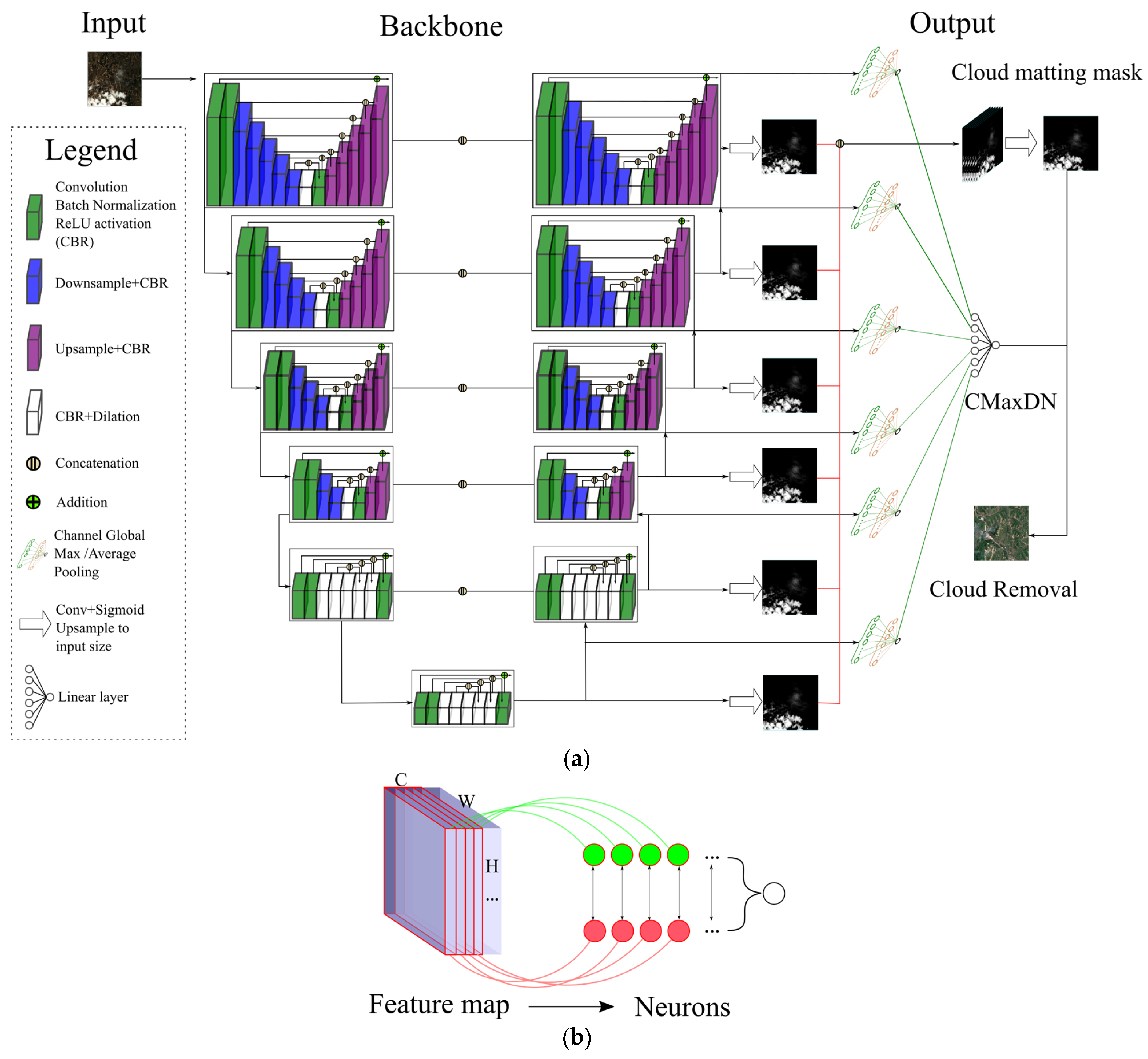
SCM-CNN employs a superior saliency detection network capable of analyzing RS images from many sizes and scenes and fusing multi-stage features. As depicted in
Figure 3a, the SCM-CNN consists of two primary components: the automatic production of the cloud-matting mask and the slice maximum digital number estimation. SCM-CNN’s backbone network is U
2Net [
46], and the RSU (Residual U-block) is employed for feature extraction and feature fusion. The traditional Residual block (RES) can be expressed as
, where
denotes the mapping result of the input feature’s expectation;
denote the two-weight layers, respectively. Each residual operation of RSU adopts a U-shaped structure, and the overall operation of RSU is expressed as
. Each residual operation yields global multi-scale features, and the RES module is superior in the model perception field and feature redundancy. The FLOPs of the RSU module are similar to the RES module, which can be faster for training and model inference (15FPS, with the input size of 512 × 512 × 3 on P4000 GPU). The model reference Feature Pyramid Networks (FPN) structure has 12 outputs, and a total of 14 outputs are obtained after further stacking to obtain two outputs of fusion features. Seven outputs represent the cloud-matting mask, and the others represent the CMaxDN value.
The CMaxDN is a piece of intrinsic information contained within the feature map. However, using the convolutional branch to perform operations based on the feature maps leads to a considerable increase in computational complexity since there are a large number of feature maps. To simplify the calculation process and obtain the CMaxDN value comprehensively based on multi-channel feature maps, we have designed a structure known as “Channel Global Average/Max Pooling”, as shown in
Figure 3b.
Typically, the CMaxDN value approached the global brightest value. Therefore, we used global max pooling to obtain the brightest value of the feature map. However, there are times when CMaxDN was greater than the brightest value of the feature map, such as in the case of low cloud opacity. In these scenarios, we hope that the model could extract more realistic CMaxDN values from the feature map. Consequently, we utilized global average pooling to summarize the feature map information.
In addition, we incorporated two Linear layers to fuse the maximum/average pooling values obtained from each feature map. Nonlinear transformation was then performed using the Relu activation function. Finally, we fused the multiple outputs of the Feature Pyramid Networks (FPN) to obtain the predicted CMaxDN. The “Channel Global Average/Max Pooling” structure only used 7144 parameters from the essence of CMaxDN to yield excellent prediction results. It integrated features from multiple channels and could effectively assist in cloud removal tasks.
The “Channel Global Average & Max Pooling” structure consisted of two linear layers. The primary objective of the first linear layer was to calculate the global average pooling and global maximum pooling values for each channel of every feature map, with the aim of generating a condensed representation of the feature map. The second linear layer employed multiple feature map compression expressions to establish the CMaxDN value.
2.5. Loss Function
The output of SCM-CNN consisted of two parts. Thus, we use the combined loss function to evaluate the model outcomes based on pixel and structural similarity, respectively. The 1-norm’s prediction results are more precise and consistent with human visual perception than other norms. Then, Equations (5) and (6) used 1-norm to establish
and
to measure the gap between pixels for the cloud-matting mask (
) and CMaxDN value (
), respectively.
We also considered the image’s general structural similarity to improve the efficacy of cloud removal. However, the structural similarity
was not apparent. To solve this problem, we used
and
pollute the cloud-free tag image (Equation (7)) and judge the structural similarity between the contaminated image and the input image. This strategy could prevent the occurrence of a zero denominator and ensure the smooth execution of model training. “MS-SSIM” is an image quality evaluation method that combines image features with different resolutions, which may be evaluated comprehensively based on the two images’ brightness, contrast, and structural similarity [
47]. The “MS-SSIM” loss function is calculated as shown in Equation (8),
represents the scale factor,
represents the mean value of the predicted feature map and the actual image,
represents the standard deviation between the predicted image and the actual image,
represents the covariance between the predicted image and the actual image,
represents the importance between the two multipliers, and
is a constant term to prevent the divisor from being zero.
Equation (9) superimposes all the error functions to obtain the loss function used in the model training.
It is worth mentioning that this paper has seven sets of output results, thus we finally get the loss value as shown in Equation (10).
The optimization objectives of the three loss functions were distinct from each other. The common practice is to fuse multiple loss functions by linearly combining them with weights. Through careful observation and experimentation, it was discovered that
could effectively balance multiple loss functions. However, linear weighting may not always produce optimal results due to the differences in gradient direction among loss functions. Instead of using a simple linear weighting approach, this paper adopted an algorithm inspired by multi-task learning, which was suitable for optimizing multiple objectives in a single task [
48,
49,
50]. As depicted in Algorithm 1, the algorithm calculated the deviation of the gradient norm for each loss function and assigned smaller weights to those with larger deviations and larger weights to those with smaller deviations. This ensured that loss functions with larger gradients do not dominate during model updates, thus ensuring equal attention is given to all loss functions.
| Algorithm 1 Automatic weighting of loss functions |
| Input: [loss1.loss2], Model, Learning Rate: |
| Output: Model |
| 1: |
|
| | %CALCULATE THE GRADIENT OF ALL LOSS FUNCTIONS |
| 2: |
|
| | %FAN OF THE GRADIENT OF THE LOSS FUNCTION |
| 3: |
|
| | %AVERAGE OF THE NORM OF THE GRADIENT OF THE LOSS FUNCTION |
| 4: |
|
| | %DEVIATION FROM THE NORM OF THE GRADIENT OF THE LOSS FUNCTION |
| 5: |
|
| | %CALCULATE THE WEIGHTS ACCORDING TO THE DEGREE OF DEVIATION |
| 6: |
|
| | %NORMALISATION OF THE OBTAINED WEIGHTS |
| 7: |
|
| 8: |
|
| 9: |
|
| | %CALCULATE THE WEIGHTED GRADIENT |
| 10: |
|
| | %UPDATE THE MODEL PARAMETERS ACCORDING TO THE GRADIENT |
| 11: |
|
| 12: |
|
| 13: |
|
| 14: |
|
2.6. Evaluation Metrics
We evaluated the model output and actual samples using metrics based on pixel similarity and structural similarity. Three major types of evaluation metrics were used. (1) The mean square error MSE (Equation (11)) was used to verify the computational accuracy of cloud opacity directly; the actuarial accuracy of the CMaxDN and pixel gap between the synthetic cloud image and the input image was denoted as
,
and
, respectively. (2) The peak signal-to-noise ratio PSNR (Equation (12)) and structural similarity SSIM (Equation (13)) were used to measure the structure of cloud opacity, synthetic cloud image, and actual sample. The disparity was noted as
,
,
, and
, respectively. (3) Accuracy (Equation (14)) was used to measure the classification approximation of cloud opacity and was noted as
.
In Equations (11)–(14), represents the prediction image, represents the reference image, and represents the mean of the predicted image and the reference image, respectively. represents the standard deviation between the predicted image and the reference image, respectively. represents the covariance between the predicted image and the reference image, is a constant term to prevent the divisor from being 0, and represents the TruePositive, FalseNegative, TrueNegative, and FalsePositive, respectively.
3. Results
This paper presented a novel deep learning-based matting model named SCM-CNN, which significantly improved the accuracy of cloud removal in visible imagery. However, existing cloud removal techniques, such as image interpolation and enhancement, have shown fewer promising results compared to the chosen two categories, which were compared in this study. (1) Atmospheric transport models, “Dark Channel” [
22], and “HOT” [
23]. (2) Image element reconstruction, “SpA-GAN” [
24,
27], “Pix2pix” [
28], and “CR-GAN” [
26]. Additionally, a standard image-matting method: “Closed-form matting” [
51].
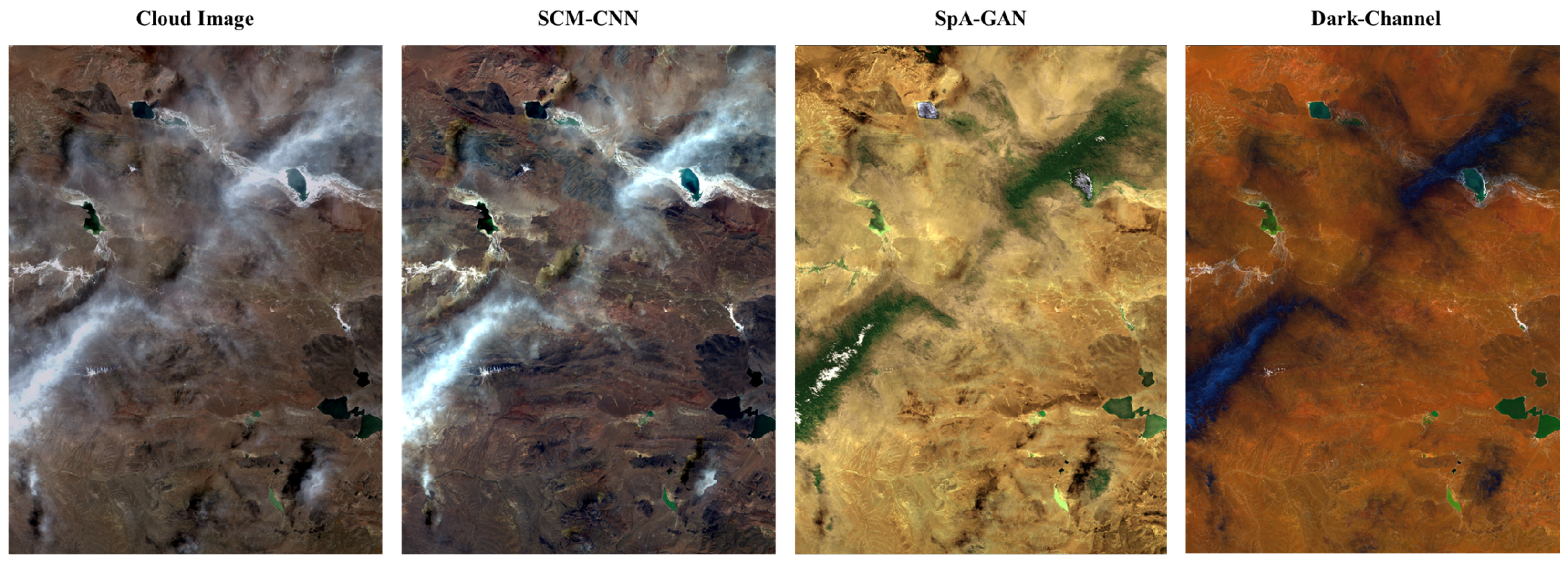
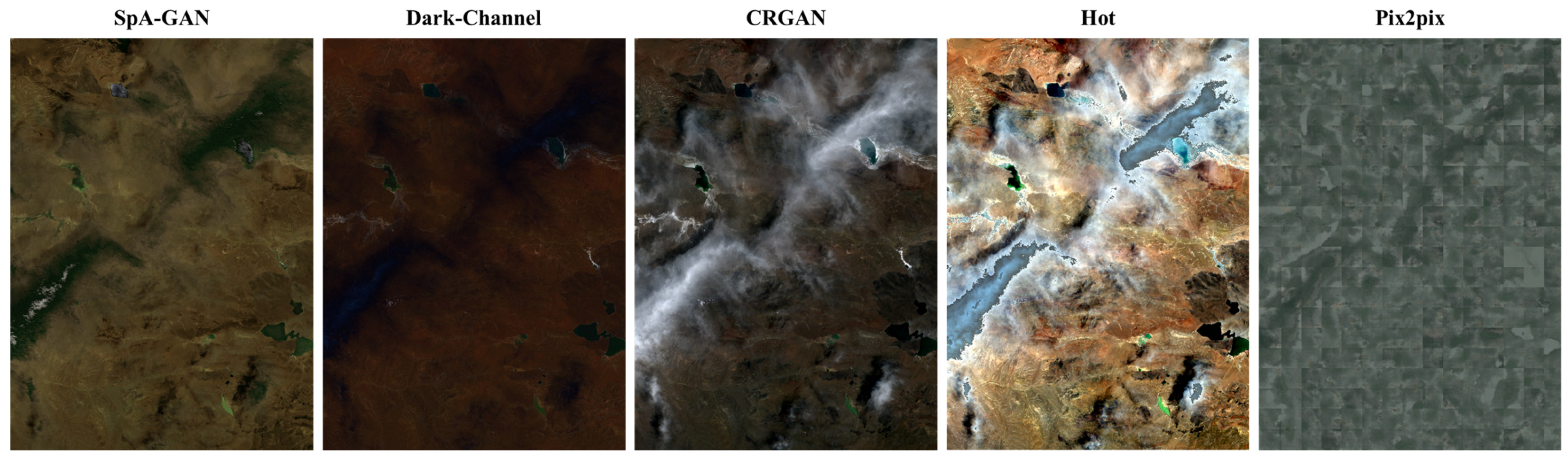
However, the usage of “Trimap” as prior input in “Closed-form matting” poses a significant challenge in practical applications. Nevertheless, because of the “Closed-form matting” strong deductibility, it only proves the feasibility of cloud removal based on matting in simulated data sets. “Hot”, “Pix2pix”, and “CRGAN” have all failed and will cause damage to the original image. Limited to space, we put this part of the results and the initial results of “Dark Channel” and “SpA-GAN” in
Figure A1.
In
Figure 4, “SCM-CNN”, “Pix2pix”, “CR-GAN”, and “SpA-GAN” are trained using the simulated dataset. The cloud removal effect of “SCM-CNN” is generally better than other methods, and “SpA-GAN” has an excellent cloud removal effect, and there is almost no color difference between slices. The cloud removal effect of “Dark Channel” is second only to “SpA-GAN”. Below that, the image changes with “Dark Channel” and “SpA-GAN”; although the clouds are removed, the overall amount of information changes significantly, and brighter objects such as roads and snow become uniform. Neither “Dark Channel” nor “SpA-GAN” can accurately obtain the cloud mask and cannot achieve post-filtering in thick cloud regions, seriously impacting its practical application. In contrast, “SCM-CNN” can generate better cloud opacity information and removal results, and image colors remain pristine.
Due to differences in time, atmosphere, lighting, and other factors in each RS image, the hue and saturation of the image may vary significantly. Methods such as histogram matching can make image colors look similar, but they also reduce the realism of image elements. Therefore, considering the above factors,
Table 1 only uses the “Cloud Image” as the noise image and the prediction result as the denoising result to measure the cloud removal effect of the image roughly with the PNSR function. However, the evaluation score is very different from human visual perception.
Figure 4 shows the usefulness of SCM-CNN for removing real RS image clouds, but evaluating the quality of RS image cloud removal results is challenging. Therefore, this work focuses on the validation of simulation data sets.
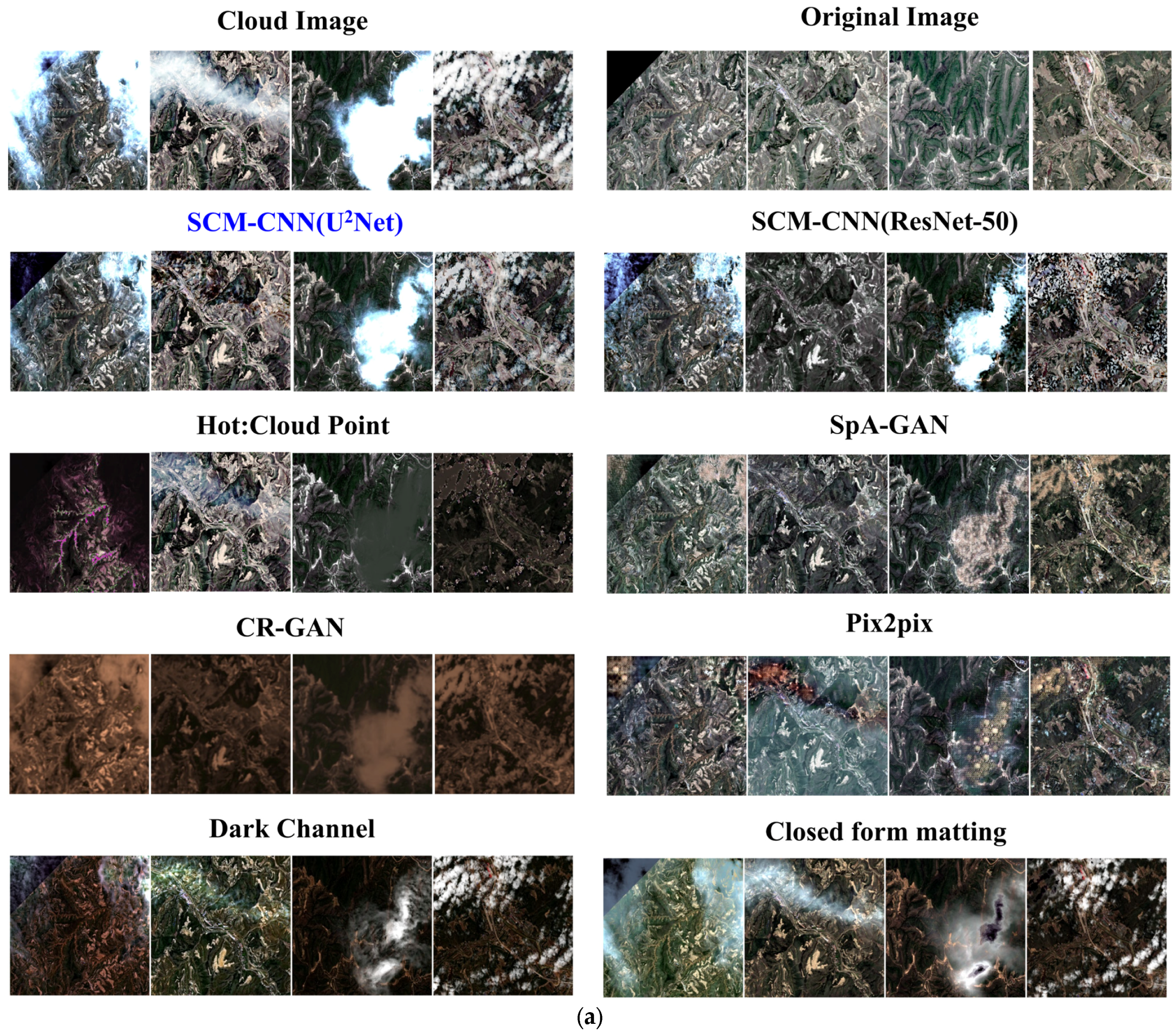
In
Figure 5a, the “Trimap” was employed as an input to direct the “Closed-form matting” method. The “Dark Channel” approach utilized a 15 × 15 filtering window for dark visual elements. “SpA-GAN”, “CR-GAN”, and “Pix2pix” are variants of CGAN (Condition Generative Adversarial Networks), with “SpA-GAN” and “CR-GAN” incorporating an attention mechanism. In this paper, the “SCM-CNN” is trained to utilize the U
2Net and ResNet-50 backbone networks, respectively. All cloud removal techniques, including deep learning and non-deep-learning methods, can produce superior results when only thin clouds are in the image. However, when thick and thin clouds coexist in the image, the accuracy of “CGANs” (SpA-GAN, Pix2pix, CR-GAN) decreases significantly. “HOT”, “Dark-channel”, “Closed-form matting”, and “SCM-CNN” can still assess the thin cloud zone more accurately to recover surface details.
4. Discussion
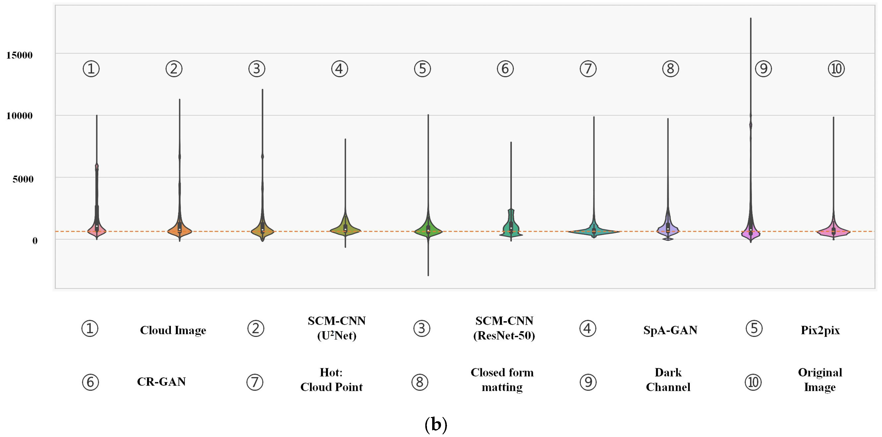
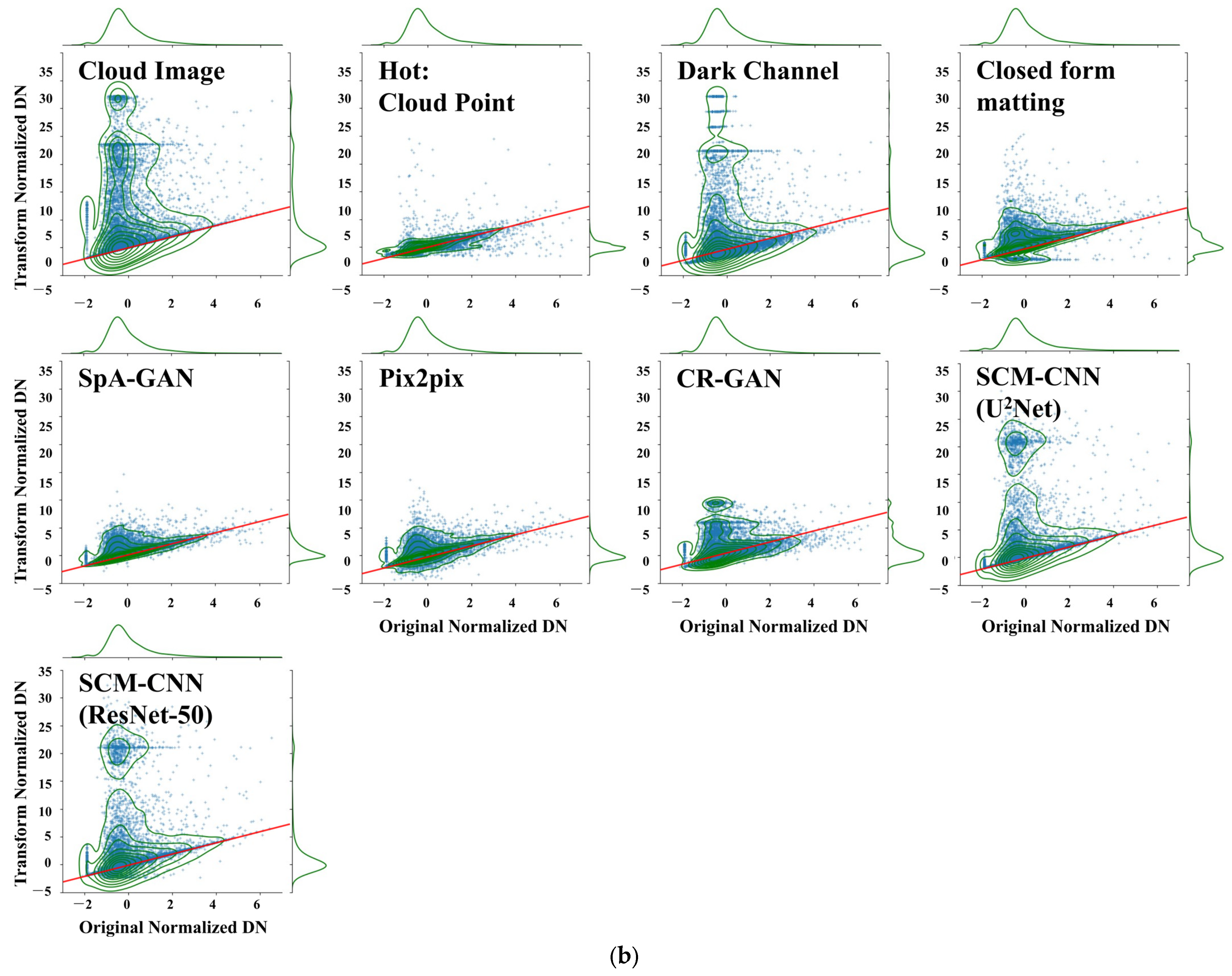
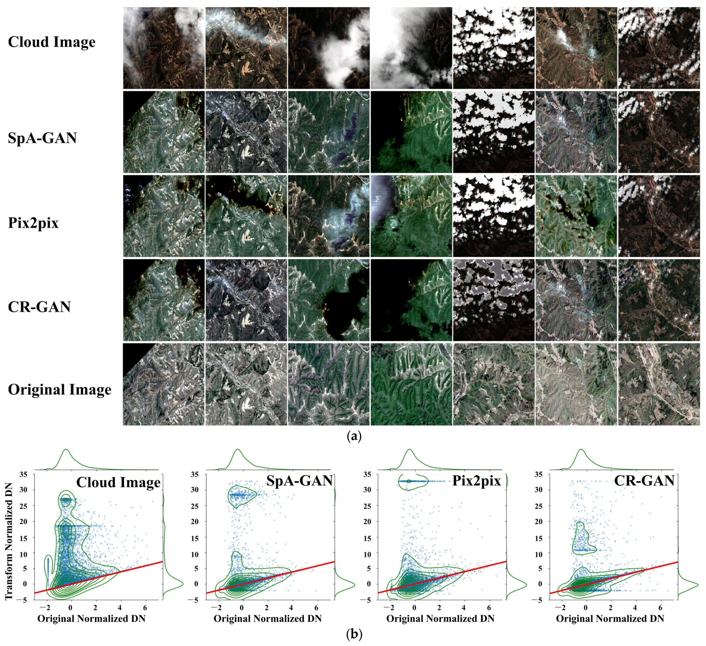
Due to cloud contamination, the local pixel features of the synthesized cloudy image are altered in
Figure 5b, and the overall image has fewer dark features than bright features. However, the image elements in the uncontaminated region will preserve their original distribution characteristics. Consequently, the primary elements continue to be dispersed around the orange dashed line. Based on the various model outputs, we can make the following preliminary assessment:
The “Hot” method adjusts the pixel brightness distribution by setting the unmistakable skyline. Therefore, the model is more sensitive to the ground feature, leading to variable variations in the unmistakable skyline, and it is prone to over-correction and color distortion.
Because of differences between traditional and satellite RS images (Refer to
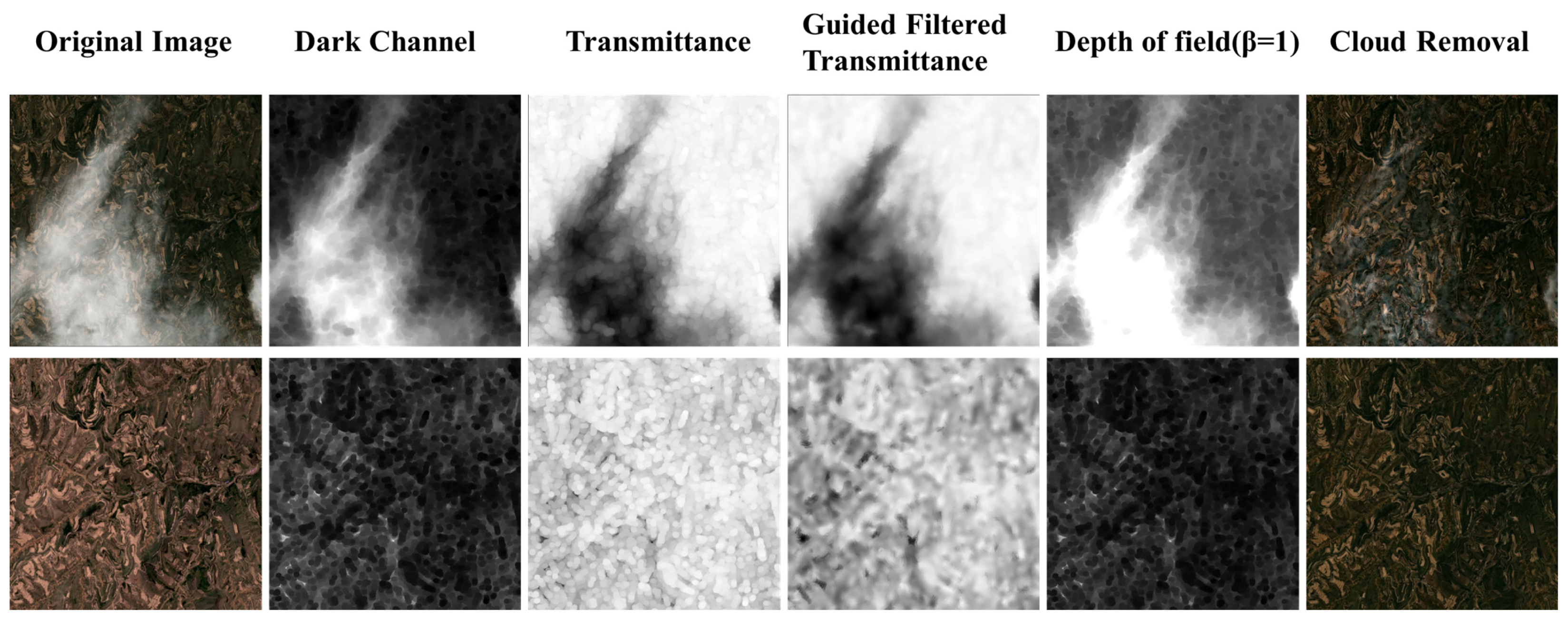
Figure A2 for details). “Dark Channel” will cause the image’s overall color to darken.
“Closed-form matting” demonstrates the feasibility of matting in remote sensing image cloud removal, which uses the color line model and ridge regression optimization algorithm. However, this method requires an accurate “Trimap” as an a priori input, significantly limiting the applicable scenarios.
“SpA-GAN”, “Pix2pix”, and “CR-GAN” are advanced conditional generative adversarial models. However, the most crucial point is that partial pixel loss may lead to multiple entities may be invisible in RS images. Therefore, the generative adversarial network can show significant distortion in areas covered by thick clouds.
“SCM-CNN (U2Net)” and “SCM-CNN (ResNet-50)” receive good cloud removal results, with almost no color deviation from the original image. The reason is that “SCM-CNN” is based on image-matting, which embedded cloud detection. The cloud removal results of the “SCM-CNN (U2Net)” model are more reliable. Additionally, with more accurate cloud opacity estimation and less patchiness. This further demonstrates the superiority of our chosen saliency detection network.
To summarize, the different approaches to cloud removal substantially alter the values of image elements, even in the areas of the image that are free from clouds. Consequently, meeting the requirements for secondary production is a challenging task. On the contrary, the “SCM-CNN” technique identifies clouds preferentially, produces cloud opacity and CMaxDN data, and then employs the Image matting formula to restore the image after removing the clouds. Therefore, the outcomes are highly dependable and do not alter the image elements in the cloud-free regions.
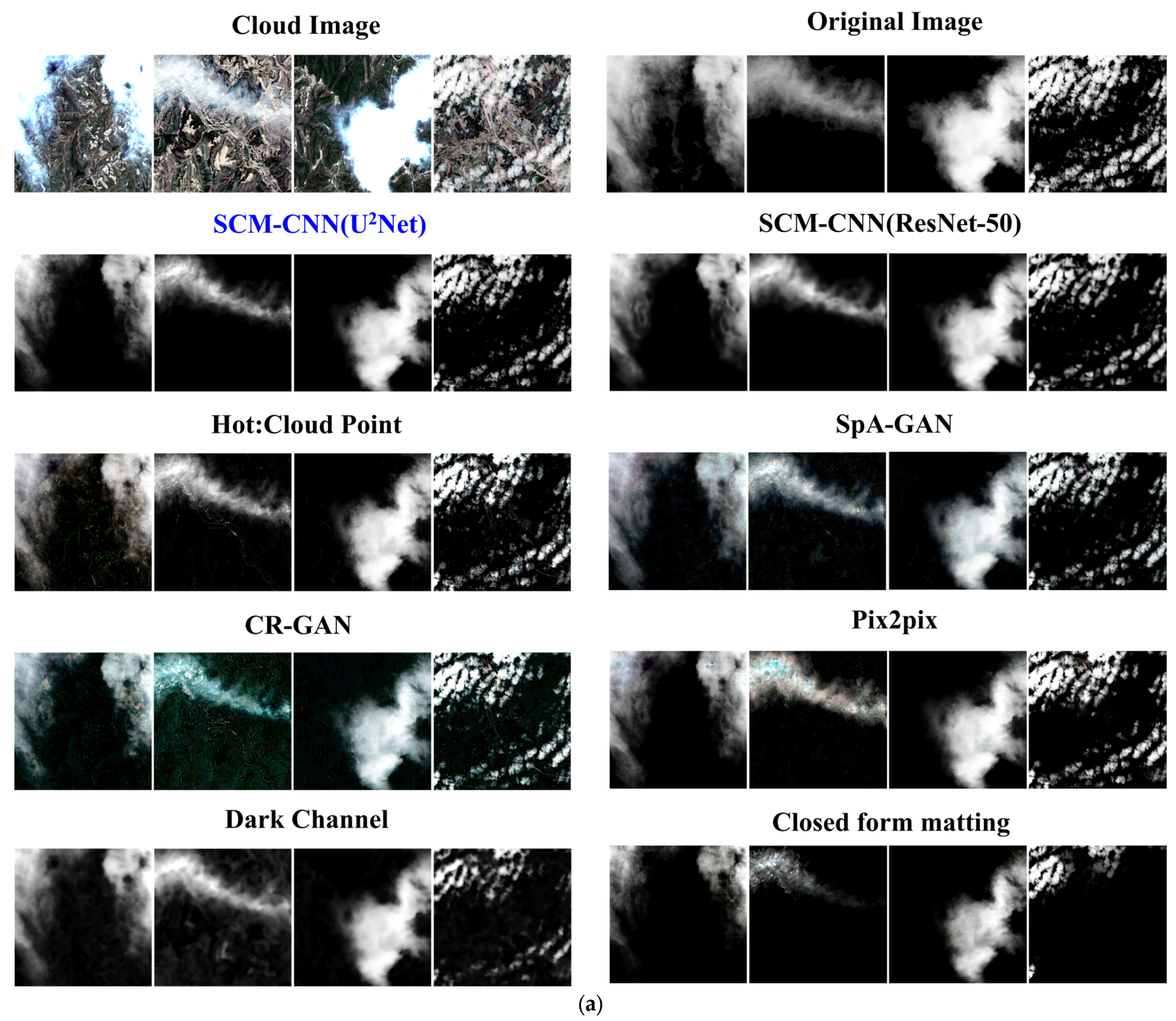
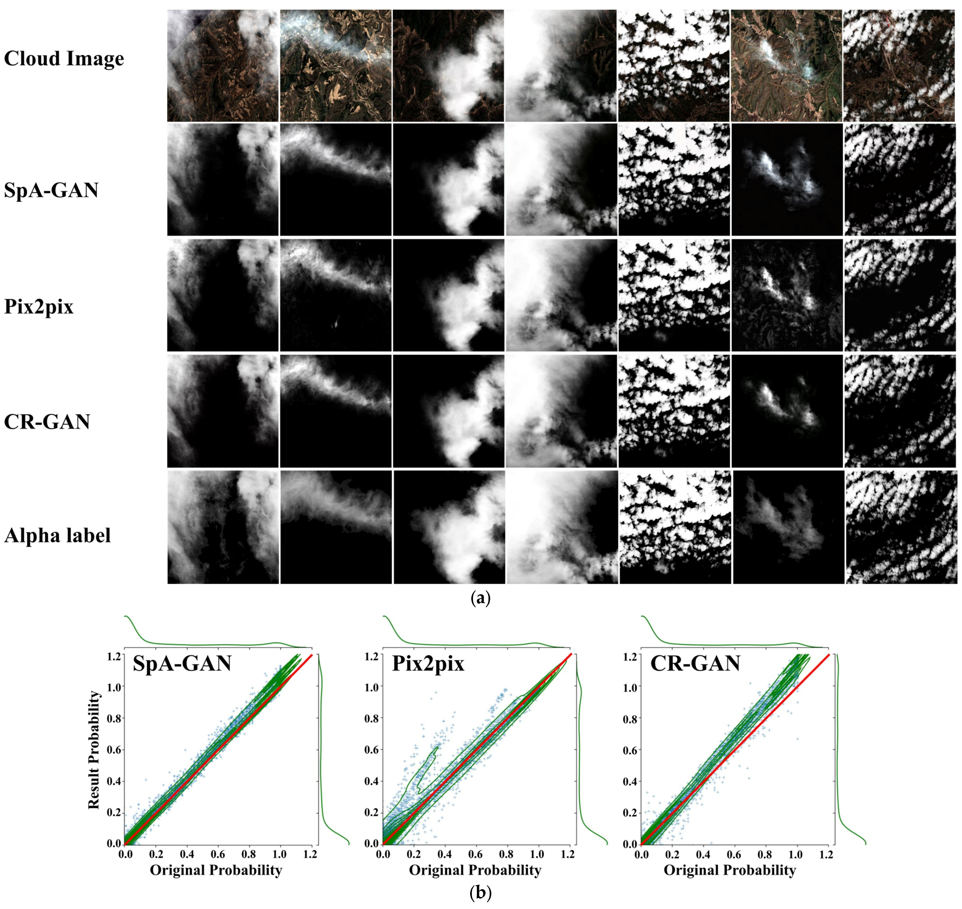
Figure 6a,b represent the results from the estimated image of cloud opacity to intuitively evaluate the quality of image de-clouding. Due to Equation (3), theoretically, all the calculated
values are greater than or equal to 0. However, the “Hot”, “Dark Channel”, and “CGANs” will have unreasonable values, and we set the
values to
and the
values to
. Since the noisy background of the image no longer limits it, it can reflect the effect of model cloud removal more intuitively.
Visual observation can evaluate from two essential points: 1. The purity of the image. 2. The light and dark changes of the image. The purity of the image reflects the effect of foreground rejection during the cloud opacity operation, and the higher the purity the lower the noise of the cloud removal result. On the contrary, the cloud removal process will significantly modify the background image elements. The light and dark changes in the image reflect the accuracy of the cloud opacity calculation, and the closer to the label the higher the accuracy. The combined performance is that
Figure 6a has higher clarity and contrast, and
Figure 6b’s scatter points are clustered around the red line. With careful consideration of the purity and the light and dark changes of the images, “U
2Net” is better than “ResNet-50”as the backbone.
Nevertheless, biases based on visual interpretation, such as “SpA-GAN”, can deceive human vision more effectively by replacing cloud-contaminated image elements with those of a similar hue. However, there is a significant discrepancy between the simulated and actual surface information. To precisely measure the cloud removal effect, we begin the mathematical statistic comparison by validating the cloud removal and cloud opacity estimation results.
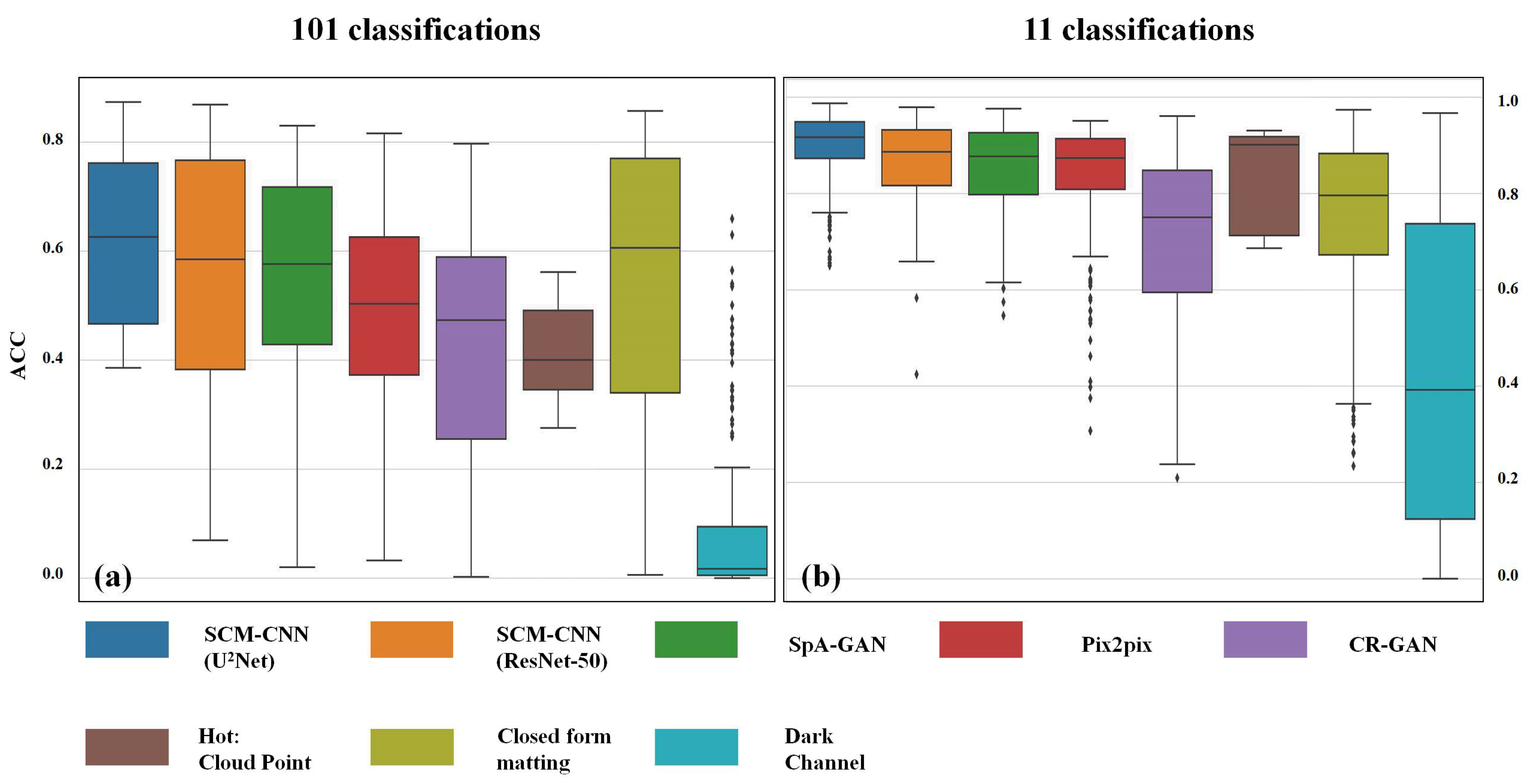
We developed only 20 sets of typical image slices for statistical purposes because the Hot technique requires manual screening operations and is less automated. Other methods employed 640 sets of image slices to assess the model’s performance based on image element similarity RMSE, structural similarity SSIM, peak signal-to-noise ratio PSNR, and classification accuracy ACC, respectively. The evaluation outcomes are presented in
Table 2 and
Figure 7.
Table 2 displays the various classification metrics produced for cloud removal and opacity estimation images using various methods. “CGANs” map the cloudy image element into the cloud-free image distribution characteristics, minimizing the difference between the cloudy image element and the cloud-free image element. However, the reflection characteristics of the image element are not identical to the semantic information. Therefore, “GANs” contribute to the deceptive image element of the metrics and the low reliability of the direct measurement of cloud removal findings. Consequently, we perform the metrics operation based on each model cloud opacity image. The estimations of cloud opacity, namely, RMSE (Alpha), SSIM (Alpha), and PSNR (Alpha), demonstrate that the efficacy of “SCM-CNN (U
2Net)” surpasses that of other methods by a significant margin, while “SCM-CNN (ResNet-50)” also achieves commendable results. On the other hand, although Hot and CGANs exhibit better RMSE (Alpha) scores in terms of image element similarity, their performance in the structural similarity index SSIM (Alpha) is generally subpar.
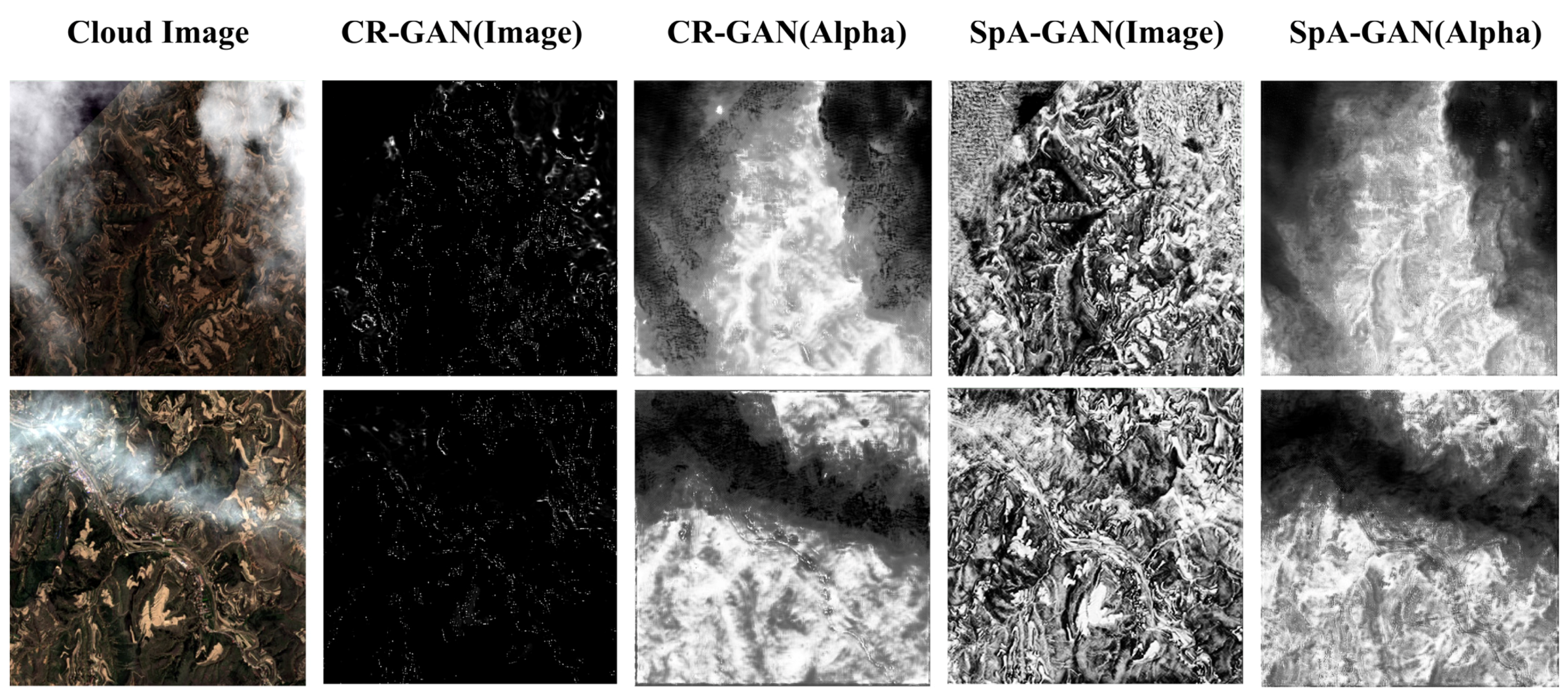
In addition, “Hot” and “CGANs” also modify many image elements in the original image’s cloud-free region, resulting in many noise points in the cloud opacity estimation map. “SpA-GAN” output results are very similar to the global features, and the obtained ones are filled with a large number of ground surface texture features, but the pixel gap is small.
Figure 7 divided the prediction results into 101 and 11 classes based on intervals from 0–1, and then obtained the prediction pixel accuracy based on matching the prediction results to labels. In
Figure 7, the ACC101 (Alpha) shows that “SCM-CNN” has the best performance, while CGANs and Closed-form matting metrics are unstable. In addition, ACC11 (Alpha) shows that each method of cloud removal possesses better accuracy and the probability density of CGANs is more concentrated on a particular part.
The disadvantage of “Dark Channel” transmittance estimation is that it does not conform to the imaging mechanism of RS images and will enhance or weaken the image according to the image element brightness. The “Hot” is more sensitive to the feature, leading to the apparent skyline variation. The magnitude is variable, and all the image elements that deviate from the clear skyline must return to the clear skyline, but this step introduces much noise. The methods employed in this study for image generation are known as conditional generative adversarial networks (CGANs), which are currently considered state-of-the-art. The comparison of the three CGANs utilized in this study, SpA-GAN, CR-GAN, and Pix2pix, indicates that the overall effect of SpA-GAN is greater than that of CR-GAN and Pix2pix. This is primarily due to the attention mechanism introduced by SpA-GAN and CR-GAN. For more details, please refer to
Figure A5, which presents the attention images under different conditions. However, the models cannot distinguish between thin and thick clouds. When complex meteorological conditions occur, the model results appear to be “fabricated,” reducing the realism of the cloud removal results. In contrast, our proposed “SCM-CNN” is based on cloud detection, which achieves cloud removal by estimating clouds’ opacity and maximum reflectance in RS images without modifying the image elements in cloud-free areas.
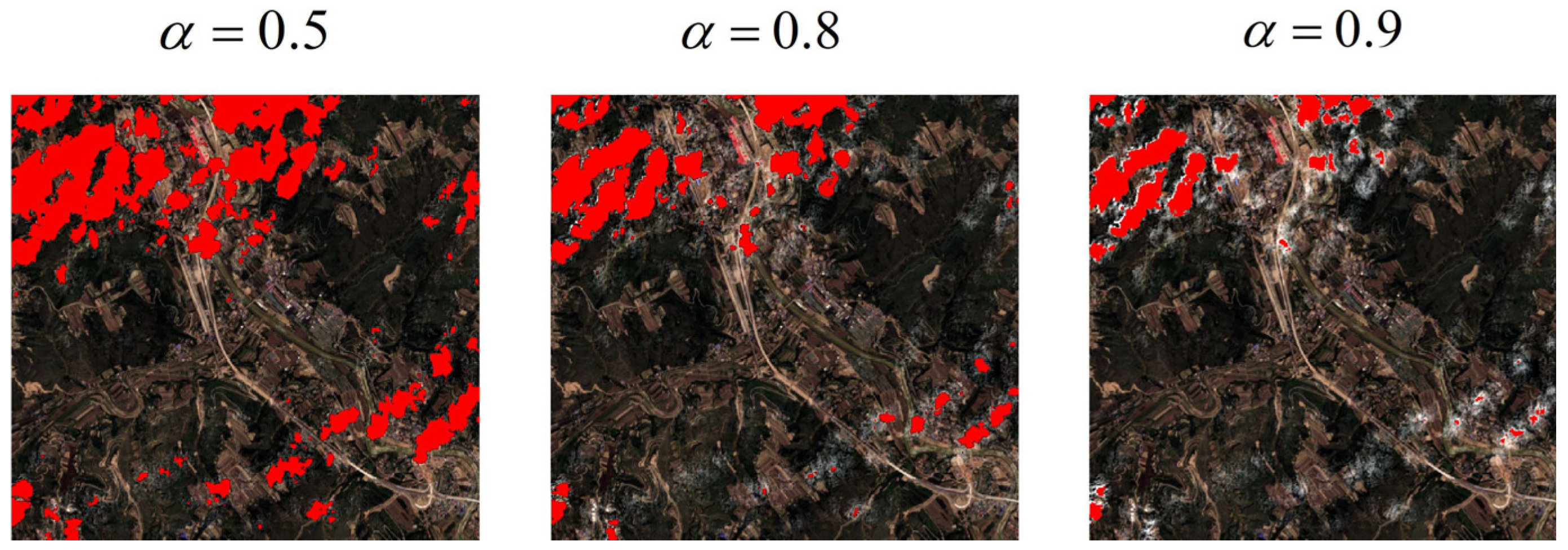
In addition, it is worth mentioning that as the cloud opacity increases, the confidence level of the surface image elements recovered results will gradually decrease. Depending on the scenario, “SCM-CNN” can be artificially set as a threshold in practical applications to assist human interpretation and data processing (
Figure 8).
“SCM-CNN” demonstrates considerable generalization and stability in removing clouds from a single image, but it still has some shortcomings. Firstly, it is worth noting that the Sentinel-2 image data are Uint16, and the upper limit of image reflection brightness is variable. To normalize the training sample, we divide the atmospherically corrected Sentinel-2 image by 10,000. However, since the reflection value of the data obtained in this way is generally small, we will use “z-score” normalization to organize the data in the subsequent study to improve its universality. Secondly, the simulated data resemble natural remote sensing imagery, and the model can be effectively transferred to natural Sentinel-2 satellite imagery cloud scenes. However, the model presents some blurry artifacts in the cloud shadow areas of remote sensing images due to shadow issues being neglected. Thirdly, to achieve accurate estimation and removal of cloud opacity, this paper employs a backbone network based on saliency detection and a multi-scale feature extraction and fusion strategy. Compared with existing algorithms for thin cloud removal, SCM-CNN can remove thin clouds better under the condition of coexisting thin and thick clouds. Therefore, it has good applicability for the frozen zone with severe fog and cloud cover. However, the model still exhibits some misjudgment when clouds are located above highly reflective ice and snow, typically recognizing highly reflective snow as thick clouds.
In the following research, we propose adopting strategies to optimize the algorithm: 1. Replace the CNN network with the Transformer network, which has performed better in recent years to achieve the attention mechanism and multi-scale feature fusion [
52]. 2. Collect heterogeneous region image base map to improve the robustness of the model. 3. Fuse more wavebands and other auxiliary information (DEM, DSM, and others.) from RS images into the model to achieve higher accuracy of cloud-snow differentiation. 4. Replacing “Channel Global Average & Max Pooling” with an MLP-Mixer may lead to better generalization and accuracy improvements [
53].
5. Conclusions
In this research, we approached the subject of single-frame RS image cloud removal from the image-matting angle. Moreover, we discussed the principles, advantages, and disadvantages of various single-frame image cloud removal methods. We established an open-source “SCM-CNN” model and supporting data.
We can draw the following conclusions from the research results: 1. Single-frame RS image cloud removal can only recover the surface information covered by thin clouds. Then, improving model stability in thick and thin cloud scenes is very important. 2. “SCM-CNN” adopts a saliency detection network, multi-scale extraction, and the fusion of image features to achieve high-precision cloud opacity generation. Furthermore, the cloud removal process is more consistent with the imaging mechanism of RS images. 3. “SCM-CNN” is based on cloud detection, and the results of cloud removal do not interfere with the original images of cloud-free areas. 4. A synthetic data set is created. All cloud removal methods can operate efficiently on our datasets. 5. The effect of the “SCM-CNN” method is significantly better than other comparison methods. It is worth mentioning that CGANs’ image element reconstruction ability is powerful, thus it is easy to obtain similar but not identical image elements. 6. Changing the conditions of “CGANs” can also obtain better cloud opacity estimation results (
Figure A3 and
Figure A4). Thus, cloud matting can be effectively migrated to other types of deep learning models.
Above all, “SCM-CNN” can effectively build the cloud opacity information from single-frame RS images. Moreover, “SCM-CNN” demonstrates good anti-interference performance in the coexistence of thick and thin clouds. Cloud matting is very helpful for remote sensing image processing in cloudy areas, and we will continue to intensify our efforts in this area.


 ,
, 


