
Multi-Temporal Trend Analysis of Coastal Vegetation Using Metrics Derived from Hyperspectral and LiDAR Data


1
U.S. Army Corps of Engineers, ERDC, Wetlands and Environmental Technologies Research Facility, Lafayette, LA 70504, USA
2
U.S. Army Corps of Engineers, ERDC, Geospatial Data Analysis Facility, Vicksburg, MS 39180, USA
3
U.S. Army Corps of Engineers, ERDC, Joint Airborne Lidar Bathymetry Technical Center of Expertise, Kiln, MS 39556, USA
*
Author to whom correspondence should be addressed.
Remote Sens. 2023, 15(8), 2098; https://doi.org/10.3390/rs15082098
Submission received: 9 March 2023
/
Revised: 11 April 2023
/
Accepted: 12 April 2023
/
Published: 16 April 2023
(This article belongs to the Special Issue Seasonal Vegetation Index Changes: Cases and Solutions)
Abstract
:Monitoring and modeling of coastal vegetation and wetland systems are considered major challenges, especially when considering environmental response to hazards, disturbances, and management activities. Remote sensing applications can provide alternatives and complementary approaches to the often costly and laborious field-based collection methods traditionally used for coastal ecosystem monitoring. New and improved sensors and data analysis techniques have become available, making remote sensing applications attractive for evaluation and potential use in monitoring coastal vegetation properties and ecosystem conditions and change. This study involves the extraction of vegetation metrics from airborne LiDAR (Light Detection and Ranging) and hyperspectral imagery (HSI) to quantify coastal dune vegetation characteristics and assesses landscape-level trends from those derived metrics. HSI- and LiDAR-derived elevation (digital elevation model) and vegetation metrics (canopy height model, leaf area index, and normalized difference vegetation index) were used in conjunction with per-pixel linear regression and hot spot analyses to evaluate hurricane-induced spatial and temporal changes in elevation and vegetation properties. These assessments showed areas with greatest decreases in vegetation metric values were associated with direct tropical storm energies and processes (i.e., overwashing events eroding beach and dune features), while those with the greatest increases in vegetation metric values were in areas where overwashed sediments were distributed. This study narrows existing gaps in dune vegetation data by advancing new methodologies to classify, quantify, and estimate critical coastal vegetation metrics. The tools and methods developed in this study will ultimately improve future estimates and predictions of nearshore dynamics and impacts from disturbance events.
1. Introduction
Coastal landscape features (e.g., beaches, dunes, wetlands) provide benefits that range from regulating services (floods, drought, and land degradation), supporting services (soil formation and nutrient cycling), and provisioning services (food and fresh water), to maintaining high biological productivity and serving as critical habitat for fish and wildlife. Coastal dunes also yield substantial economic benefits by reducing damage to residential and commercial infrastructure during significant storm events. However, these dynamic environments are inherently vulnerable and geomorphologically unstable by nature of their position at the interface of land and sea [1]. While coastal beach, dune, and wetland features frequently undergo nominal changes due to natural fair-weather pressures (i.e., wind, waves, and tides), the effects of climate change, especially large storms and irregular weather patterns, can induce significant shifts in the state, evolution, and dynamics of these features, thereby increasing the susceptibility of these systems to destructive erosional forces [2,3]. Therefore, many restoration activities and coastal reconstruction projects focus on dune resiliency to help reduce the risk to coastal communities [4].
Vegetation is a critical biotic component of coastal ecosystems since they have direct and indirect impacts on system stability and resilience [1]. Plants can contribute to erosion control through their above- and belowground components. For example, high leaf-area and stem densities in aboveground plant mass can reduce rain and wave splash impacts, mitigate storm surge, and diminish near-bed shear stresses, as well as facilitate vertical and horizontal accretion through organic matter accumulation and sediment trapping [5]. Belowground root mass can also increase the sheer strength of the substrate and thereby prevent erosion by resisting structural failure and creating shore bathymetric profiles that assist in dissipating wave energy [6]. Therefore, within the coastal ecosystem, dune vegetation productivity and processes play a complex and vital role in shoreline stability and wetland resilience [6]. Estimating vegetation characteristics (i.e., biomass) can be essential for monitoring and predicting wetland productivity, resilience, and ecosystem health [7,8]. Thus, rapidly quantifying vegetation dynamics across the dune profile (from the dune toe to beyond the more elevated and heavily vegetated primary dune) is an important aspect for understanding dune morphology and associated impacts from coastal processes [9].
Recent studies have focused on evaluating physical and biological processes and the long-term evolution of coastal systems as functions of natural processes and anthropogenic activities [7,10,11]. Although some emphasis has been on coastal vegetation monitoring and influence on erosion potential, fewer studies have directly evaluated correlations to vegetation structural properties (i.e., vegetative densities), presumably in part due to limited and insufficient data to support these efforts. Similarly, there are data and knowledge gaps regarding required vegetation inputs to coastal numerical models, particularly for large-scale or regional coastal projects, resulting in many models incorporating synthetic vegetation data or constant values as inputs [12]. Despite ongoing improvements, monitoring and modeling are still considered major challenges in anticipating environmental response to hazards, disturbances, and management activities.
Some major challenges associated with monitoring of coastal wetland landscapes are the cost and laborious nature of traditional ground-based data collections. Remote sensing systems and applications have been shown to provide cost-effective and more efficient alternatives and complementary approaches to ground-based collections and assessments [13]. However, monitoring wetland landscapes and measuring vegetation biophysical and biochemical properties using traditional broadband sensors (usually up to six spectral bands) [14] can be limited (due to spectral resolution) and ineffective (due to the underlying soil types, canopy and leaf properties, and atmospheric conditions), leading to asymptotic saturation for some vegetation metrics [8,15]. Other challenges associated with the monitoring of coastal landscapes are related to the quantification of changes in vegetation structure or function at scales (i.e., spatial, spectral, and temporal) necessary to adequately evaluate system stability. However, studies have shown that narrowband data (i.e., hyperspectral imagery [HSI]) are more sensitive to differences in energy wavelengths and have higher potential to detect subtle variations in vegetation characteristics, as compared to broadband multispectral imagery [15,16,17,18]. Higher spectral information is useful for estimating important vegetation photosynthetic activities and canopy structural variations [19]. Similarly, Light Detection and Ranging (LiDAR) data can provide efficient and effective alternatives to ground-based structural measurements. Some LiDAR sensors can penetrate vegetation cover to obtain estimates of relative heights above ground and detailed vegetation structure parameters (depending on point spacing) [20,21,22]. Using high-resolution HSI imagery in conjunction with LiDAR data can assist in discriminating plant species, determining biomass distribution, and extracting key coastal dune vegetation metrics [23,24,25,26], all of which are useful in monitoring and modeling changes in expansive wetland ecosystems [27].
The goal of this study was to develop simple but effective methods for mapping and monitoring coastal vegetation properties within the dune complex by capitalizing on recent sensor improvements, analytical techniques, and the temporal resolution of data collected by the U.S. Army Corps of Engineers’ (USACE) National Coastal Mapping Program (NCMP). The USACE NCMP provides regional, repetitive, high-resolution, high-accuracy elevation and imagery data that are useful for assessing changes and trends in geomorphological and environmental properties. Therefore, the objectives of this study were to (1) develop tools to semi-automate metric extraction from NCMP LiDAR and HSI data to quantify dune vegetation biological characteristics; and (2) use a pilot study to demonstrate how derived metrics can be utilized to evaluate and compare spatial and temporal changes in vegetation properties, whether due to episodic events (i.e., hurricane impacts) or natural processes. This study advances existing dune and wetland system knowledge and remote sensing techniques by utilizing spatially and temporally coincident HSI and LiDAR data for developing new tools to more efficiently classify, quantify, and estimate critical dune vegetation metrics, thereby improving future estimates and predictions of storm processes and impacts.
2. Materials and Methods
2.1. Study Area
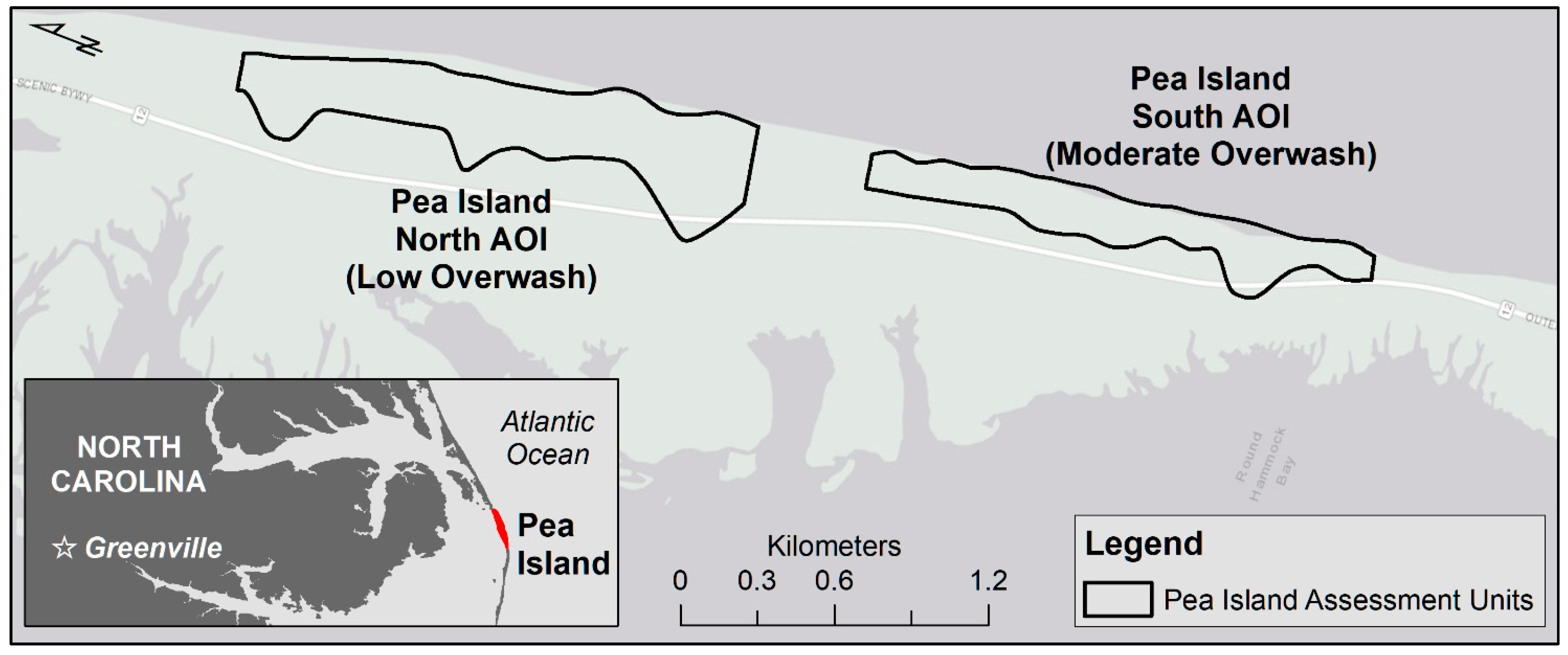
The study site (Figure 1), which is located on Pea Island in the Outer Banks of North Carolina, United States (approximately 170 km east of Greenville), was chosen to evaluate methods for extracting dune vegetation (DuneVeg) metrics, develop an automated workflow for remote extraction techniques, and perform a trend analysis using the derived vegetation metrics. The site is part of the US Coastal Research Program’s DUring Nearshore Event eXperiment (DUNEX), which is a multi-agency, academia, and stakeholder collaboration to study nearshore processes during coastal storm events [19,21,22]. The Pea Island site is part of the Pea Island National Wildlife Refuge and is approximately 19 km in length and 2.4 km wide.
2.2. Vegetation Metric Extraction
2.2.1. Airborne Hyperspectral Imagery and LiDAR Data
This study utilized coastal HSI and LiDAR data routinely collected for the USACE NCMP to evaluate extraction methods of coastal vegetation characteristics. These data are collected by the Joint Airborne LiDAR Bathymetry Technical Center of Expertise [24] to capture existing beach and near-shore conditions along the sandy coastlines of the U.S. The NCMP uses the Coastal Zone Mapping and Imaging Lidar (CZMIL) system, which integrates a Teledyne Optech LiDAR sensor with topographic (70 kHz pulse rate) and bathymetric (10 kHz pulse rate) capabilities, a digital camera, and the Itres Compact Airborne Spectrographic Imager (CASI)-1500 on a single remote sensing platform mounted on a fixed-wing aircraft. The CZMIL HSI and LiDAR data are acquired spatially and temporally coincident and at a consistent scale and resolution in the coastal zone [27]. Thus, they represent a unique opportunity to use open-access, freely available imagery (in this case HSI) with high-fidelity LiDAR data to extract regional-scale vegetation metrics at project-relevant spatial resolutions, which is not currently possible with standard cameras or other available imagery sources.
The HSI data were collected at an altitude of 400 m across a 300 m ground swath. Although the CASI-1500 imager is a programmable sensor capable of hundreds of narrow spectral bands (288 channels at a spectral resolution of 3.5 nanometer [nm] Full Width Half Max [FWHM]), the data were collected in a 48-band configuration with a spectral range of 362 to 1045 nm at a spectral resolution of 14.4 nm (FWHM). The spectral resolution of each band was 14.4 nm, assigned at the center of the FWHM. The CZMIL system used Teledyne’s HydroFusion software suite to perform radiometric calibration processing, which includes conversion of Digital Number (DN) to at-sensor radiance, glint/ripple correction to smooth water surface effects, and conduct atmospheric corrections which convert surface radiance to surface reflectance, prior to mosaicking into 1 m spatial resolution imagery [25,26,28]. The true-color three band (RGB) collection returned higher spatial resolution imagery (approximately 5 cm ground resolution for 400 m altitude collection), which were used as ancillary data for visual accuracy and feature verification [25].
The integrated system, which was developed specifically for use in coastal mapping and charting activities, was designed to meet or exceed U.S. Geological Survey Quality Level 2 (QL2) standards for topographic LiDAR data collections, and produces a vertical accuracy ≤ 10 cm RMSEZ on land surfaces and shallow water [24]. Vertical positions from the LiDAR data were referenced to the NAD83 ellipsoid (GRS 1980) and were converted to NAVD88 orthometric heights using geoid model 12B. Seamless topobathymetric first return and bare-earth digital elevation model (DEM) grids (1 m spot spacing and approximately 19.5 cm elevation accuracy at a 95% confidence level) were produced through CZMIL processing [26,28,29].
Table 1 provides a summary of all qualifying NCMP data from the late-growing season (2016 NCMP data were collected several weeks past the typical growing season for North Carolina) [30] across the study period (2016 to 2019). These data were used to develop DuneVeg tools [31] to semi-automate vegetation metric extraction and to demonstrate how derived metrics can be used to evaluate and compare spatial and temporal changes in key vegetation properties.
2.2.2. Dune Vegetation Metric Extraction
A suite of custom geospatial processing tools (DuneVeg Toolbox, hereafter) was developed to automate the extraction of metrics from the NCMP data [31]. Using standard NCMP imagery and LiDAR products enable workflow automation to extract prioritized dune vegetation metrics in an efficient and repeatable way. The software used to develop the methodological framework for process automation was ENVI version 5.5 (L3Harris Geospatial Solutions, Inc., Broomfield, CO, USA). The ENVI Application Programming Interface (API) in IDL was used to customize ENVI functionality for automating metric extraction processes and the ENVI Py for ArcGIS module allowed for integrated access using ArcGIS Pro (version 2.3) software (ESRI, Redlands, CA, USA). The software integration allows extended capabilities that make use of spatial analytics and spectral band math algorithms to derive the vegetation metrics. Table 2 provides a list of NCMP data used in conjunction with the DuneVeg Toolbox to generate elevation and vegetation metrics.
2.2.3. Vegetation Metric: Normalized Difference Vegetation Index (NDVI)
The normalized difference vegetation index (NDVI) provides an efficient means of monitoring changes in vegetation biomass (relative biomass of live, green plants) and health. Previous studies have used NDVI data to evaluate vegetation impacts and recovery from anthropogenic, natural, and invasive disturbances [8,32,33]. Chlorophyll, the pigment in plant leaves that is used in photosynthesis, strongly absorbs visible light (from 400 to 700 nm). Conversely, the cell structure of the leaves strongly reflects near-infrared (NIR) light (from 700 to 1100 nm). The more leaves a plant has, the more these wavelengths of light are affected [34]. Previous studies have demonstrated the use of high spectral resolution HSI-derived NDVI for vegetation monitoring [35,36,37] and have shown optimal contrast between chlorophyll pigment absorption (red band) and the high reflectivity of plant material (NIR band). Moreover, when leaves become stressed or otherwise diseased, they turn yellow and as such reflect significantly less in the NIR range. Because of these photosynthetic influences, the red and NIR bands are standard for calculating NDVI [38], as shown in Equation (1):
where NDVI is the normalized difference vegetation index, NIR is HSI band 35 (856 nm), the near infrared spectral band center value, and Red is HSI band 21 (656 nm), the red spectral band center value. Band assignments were based on the wavelength closest to the band center within each spectral range according to ENVI software functionality and spectral index requirements (L3Harris Geospatial Solutions, Inc.). NDVI values range from −1 to 1, where lower values (closer to −1) generally represent non-vegetated features and higher values (closer to 1) tend to represent healthy, green vegetation [39]. Therefore, the higher the NDVI value, the higher the biomass, productivity, and vigor inferred from these calculations.
2.2.4. Vegetation Metric: Density Estimation (Vegetation Cover)
Delineation of temporal dune vegetation presence and extraction of vegetation density estimates from the atmospherically corrected NCMP HSI, were performed using the ENVI Spectral Processing Exploitation and Analysis Resource (SPEAR) vegetation delineation tool. The SPEAR tool performs a density slice method based on NDVI-derived images to generate density categories. This method was used since NDVI has a strong correlation to aboveground biomass estimation [39,40]. Therefore, inferences can be made about the level of vigor and vegetation density using NDVI value ranges. The density categories estimated from this method were (1) dense vegetation (NDVI = 0.70–1.00), (2) moderate vegetation (NDVI = 0.50–0.69), (3) sparse vegetation (NDVI = 0.25–0.49), and (4) non-vegetation (NDVI = −1.0–0.24).
The output format for this analysis was ESRI polygon features (shapefiles) indicative of the NDVI threshold estimates from each vegetation density category. Once the output densities were derived, a spatial merge (geoprocessing task) was used to join the three vegetation densities (dense, moderate, and sparse) into one category representing all vegetation (polygon feature layer). Subsequently, the output of the merge operation represented vegetation presence for the image scene. Likewise, the non-vegetation layer represented vegetation absence. Wetland, submerged, or inundated areas appearing to have brown or dying (non-green) vegetation were included as non-vegetation for purposes of deriving vegetation density estimates. The resultant products of this analysis were used as mask layers for subsequent vegetation metric extraction.
2.2.5. Vegetation Metric: Leaf Area Index (LAI)
A commonly used variable for quantifying vegetation canopy is the leaf area index (LAI), which is a measure of green leaf area (m2) per unit of ground surface area (m2). In basic terms, it is the estimated (image-derived) or measured (field-derived) amount of foliage in a plant canopy. Leaf surfaces are the primary driver of energy and mass exchange. Therefore, important processes such as canopy interception, evapotranspiration, and photosynthesis are directly proportional to LAI [41]. Moreover, the amount of leaf area directly influences net primary productivity and biomass potential, and in many systems aboveground biomass can be used to estimate belowground biomass [42].
For this study, LAI was estimated from optical remote methods using the NCMP HSI and select spectral bands. The calculations were made using ENVI band algebra and a spectral indices tool specifically designed for LAI. The equation used for calculating this vegetation index is shown in Equation (2) [43]:
where EVI is the Enhanced Vegetation Index and is an important variable for estimating the LAI using remote sensing methods, especially in areas with high relative biomass. EVI is a broadband greenness index, which was calculated using Equation (3) [44]:
where G is the gain factor (2.5), NIR is HSI band 35, Red is HSI band 21, Blue is HSI band 8 (471 nm, the blue spectral band center value; all spectral bands were atmospherically corrected surface reflectance values), and the numerical coefficients (C1, C2) and canopy background adjustment (L) that ENVI uses as part of the EVI equation. The EVI is useful for optimizing the vegetation signal in areas of high LAI (very dense vegetation), and where NDVI may saturate, which can be a limitation of using NDVI alone [45]. This algorithm makes use of the blue band to correct for soil background signals and to reduce atmospheric influences such as aerosol scattering (L3Harris Geospatial Solutions, Inc., Boulder, CO, USA).
2.2.6. Vegetation Metric: Canopy Height Model
The LiDAR data were processed to generate gridded models of the topography and surface features. A 1 m DEM was created from points classified as ground returns from the classified LAS files. A DEM is a regularly spaced raster grid of elevation values of a surface terrain with non-ground points removed so the output is a surface representation of bare ground void of vegetation and other aboveground features. A Triangulated Irregular Network (TIN) interpolation method was used with rural area filtering to produce the DEM. Similarly, a 1 m Digital Surface Model (DSM) was created from points classified as non-ground using the first return points from the classified LAS file. A DSM is a regularly spaced raster grid of surface elevation values that includes vegetation and other aboveground features. The LAS files were processed using an interpolation method in ENVI that is optimized for vegetation analysis and filters points specifically for extracting vegetation heights. A vegetation canopy height model (CHM) was created by performing a subtraction (DSM—DEM) routine using band math in ENVI to derive a height model with 1 m spatial resolution. The non-vegetation polygon feature (from the density estimate calculation) was used as a mask (geoprocessing task) to exclude non-vegetation features. The CHM contains vegetation canopy height for all areas identified as vegetation within the LiDAR extent footprint.
2.2.7. Vegetation Metric: Statistical Analysis
Vertical accuracies of LiDAR-based elevation models were assessed using ground control points (GCPs) surveyed as part of an associated DUNEX study [46]. The field-based elevation measurements on Pea Island were collected using a real-time kinematic (RTK) Global Positioning System at designated island feature (foredune, dune toe, back toe, highest dune, extra dune, and landward limit) locations along transects with 100 m spacings. The mean error and root mean square error (RMSE) were calculated using the LiDAR-derived DEM elevations relative to the RTK ground survey elevations [47]. The RMSE has been previously used to quantify the accuracy of LiDAR-derived DEMs for open and sparsely vegetated coastal environments [48,49] and the mean error is a good indicator of vertical offsets in wetland landscapes [50,51].
In the absence of in situ measurements of vegetation density and biomass, ancillary imagery and visual assessments were used to evaluate accuracies in HSI-derived NDVI (as well as vegetation density and LAI, by inference). The criterion standards for validating density and biomass were constructed through vegetation presence and greenness ratings based on independent visual examination of project HSI and RGB imagery, as well as ancillary aerial photographs (e.g., National Agriculture Imagery Program imagery collected in close temporal proximity to project HSI). To assess the accuracies of the extracted vegetation metrics, the ArcGIS Desktop v10.7.1 Confusion Matrix tool was used to compute user and producer accuracies, derive Cohen’s Kappa statistic for measuring agreement, and generate an overall accuracy score. Producer’s accuracy was used to assess the probability that real on-the-ground features (based on independent visual examination) were correctly estimated using HSI-based extraction methods. User’s accuracy was used to assess the probability that features identified using HSI-based extractions were present on the ground (per individual visual estimates of density and greenness). Cohen’s Kappa was used as a general measure of inter-rater agreement or reliability [52].
Moreover, to attain comparability among vegetation metrics, statistical analyses were performed using Statistical Analysis System software version 9.2. The PROC General Linear Models (GLM) procedure was used to do a one-way analysis of variance (ANOVA) and a means separation test (Tukey’s, α = 0.01) to evaluate the significance of differences between years for each assessment unit.
2.3. Pilot Study: Multi-Temporal Trend Analysis
Storm Impacts
Deriving vegetation metrics that bracket major disturbance events (i.e., tropical storms) provides useful data for assessing episodic impacts and ecosystem resilience and recovery. A pilot study was conducted to demonstrate the use of the derived vegetation metrics for identifying and evaluating differences and trends across a range of storm-induced impacts. For trend analyses, select areas of interest (AOIs, also referred to as assessment units; Figure 1) from within the Pea Island study site were used to evaluate recent changes in elevation and vegetation properties. The AOIs were selected based on coastal and geomorphological changes related to recent storms, i.e., overwash. An overwash event occurs when storm surge overtops the foredune ridge or when the foredune ridge is eroded by prolonged wave energies [53]. Table 3 provides a list of major storms that impacted the Pea Island study site between 2016 and 2019. These storms, which ranged in wind speed from 11.6 ms−1 to 23.2 ms−1 at Pea Island, and had a maximum storm surge from 0.9 m to 1.65 m, include Hurricanes Hermine, Matthew, Florence, Michael, and Dorian [23]. Unlike major storms, which typically provide more direct and measurable impacts, these moderate and higher frequency storms can cause more subtle yet extended impacts that can be more difficult to monitor.
Very high spatial resolution airborne true-color imagery and high-resolution LiDAR-based elevation data (described in the Airborne Hyperspectral Imagery and LiDAR Data section) were used to identify hurricane-related overwash areas within the Pea Island site. The AOIs selected for this study consisted of 2 km long bins along island dunes—with widths extending from the dune toe to the furthest landward dune [46]—that experienced moderate or low overwash impacts related to tropical storms between 2016 and 2019 (Figure 1).
Vegetation-based analyses were performed for each AOI (excluding non-vegetated areas) using summary statistics and per-pixel linear regression and hot spot analyses. To evaluate and compare spatial and temporal changes in vegetation properties, the Spatial Analyst Zonal Statistics as Table tool was applied in ArcGIS to generate summary statistics (i.e., mean, min, max, range, standard deviation) for each vegetation metric, by AOI and date combination. Trends analyses were performed using the Curve Fit v10.1 [54] ArcGIS extension to conduct linear regressions across the period of record (2016 to 2019). The Curve Fit extension, which utilized the range of vegetation metric values at each pixel location (regressed over time), was used to generate raster surfaces of regression model parameter estimates, standard errors, and goodness-of-fit for each DuneVeg metric [54]. The per-pixel linear regression data, which can provide spatial representation of vegetation change over time, were used with a Getis–Ord Gi* hot spot analysis to identify areas that have been significantly impacted by disturbance events and/or may be susceptible to future pressures.
3. Results
3.1. DuneVeg Toolbox
3.1.1. Dune Vegetation Metric Products
The DuneVeg Toolbox was developed as a means of automating methodologies and standardizing target vegetation metric and elevation-based products as part of the National Coastal Mapping Program. Figure 2 shows example NCMP data and vegetation metric products from the Pea Island South assessment unit (moderate overwash). Figure 2A,B show the NCMP HSI and LiDAR (represented as digital elevation model) data, and panels C-F show examples of the canopy height model (CHM), normalized difference vegetation index (NDVI), vegetation density (VD), and leaf area index (LAI), within a portion of the Pea Island South AOI. The HSI in Figure 2A shows, from west-to-east, the Pea Island back barrier wetlands, North Carolina Highway 12, back-island dunes, fore-island dunes, and beach, respectively. Figure 2B illustrates an example of Pea Island ground elevation, represented as a DEM (last return), derived from NCMP LiDAR data. Minimum and maximum elevations (NAVD88) occurred along the back barrier wetlands and the fore-island dunes, respectively. The elevations between these extremes were occupied by the back-island dunes and beach features, which are located at moderately high and moderately low elevations, respectively.
Example CHM data, which were generated by subtracting project DEM (last return/ground) from DSM (first return) data, are shown in Figure 2C. The minimum CHM elevations correspond to unvegetated island features (i.e., beach and developed; represented by beige in Figure 2C) and the maximum elevations correspond to shrub species located between the back-island dunes and wetland zones. The locations of these shrub features, represented by the yellow and blue colors in Figure 2C, are corroborated by estuarine scrub/shrub wetlands identified in NOAA’s 10 m Coastal Change Analysis Program (C-CAP) Regional Land Cover data [55].
Figure 2D–F represent the other vegetation metrics that were generated using the DuneVeg Toolbox. Figure 2D shows NDVI, which has a well-established correlation to photosynthetic activity and plant health. Orange and red areas indicate vegetation with low plant vigor, while green and blue areas represent vegetation with higher biomass and vigor (Figure 2D). The lower NDVI areas consist of low biomass beachgrasses, while the higher NDVI areas consist of high biomass shrubs and emergent wetland plants. Figure 2E shows an example of vegetation density data that were generated using density thresholds and the NDVI data. Blue represents high density vegetation, yellow represents moderate density vegetation, and red represents sparse vegetation (Figure 2E). These vegetation density zones correspond to regions of greenness and density observed in the HSI (Figure 2A). LAI, which is an estimate of leaf productivity, is shown in Figure 2F. Red areas represent vegetation with low LAI (low leaf productivity) and greens and blues represent vegetation with high LAI (high leaf productivity). LAI values in Figure 2F correspond well to observed regions of high and low vegetation productivity (greenness and density, Figure 2A).
3.1.2. Elevation and Vegetation Metric Accuracy Assessments
The overall average vertical accuracies of the LiDAR-derived DEMs for all dates and assessment units—expressed as the mean error and RMSE—were −0.006 m (n = 1228) and 0.214 m, respectively. The mean errors for the 2016, 2018, and 2019 DEMs were −0.03 m (n = 421), −0.07 m (n = 400), and 0.08 m (n = 407), respectively. The RMSE values for the 2016, 2018, and 2019 DEMs were 0.146 m, 0.225 m, and 0.257 m, respectively. Across all dates, the average vertical accuracies of DEMs ranged from a low RMSE of 0.15 m (secondary dune features) to a high RMSE of 0.28 m (dune toe). All other features had RMSE ≤ 0.25 m. These derived errors fall within the expected range for LiDAR-based DEMs, and those reported as part of other barrier island studies [56,57].
To assess the accuracy of the HSI-derived NDVI data, a total of 180 assessment points (stratified random sample) were used across all dates and assessment units to construct a confusion matrix (Table 4). Accuracy assessments of NDVI returned minimum and maximum accuracies of 0.85 and 0.97 for the moderate and low NDVI ranges, respectively. The confusion matrix returned an overall accuracy and Cohen’s Kappa value of 0.91 and 0.87, respectively. Most misclassifications occurred in the moderate vegetation class. This is due to difficulties in differentiating moderate from sparse or dense vegetation when greenness and biomass approach class thresholds.
3.1.3. Vegetation Metric Summary Statistics
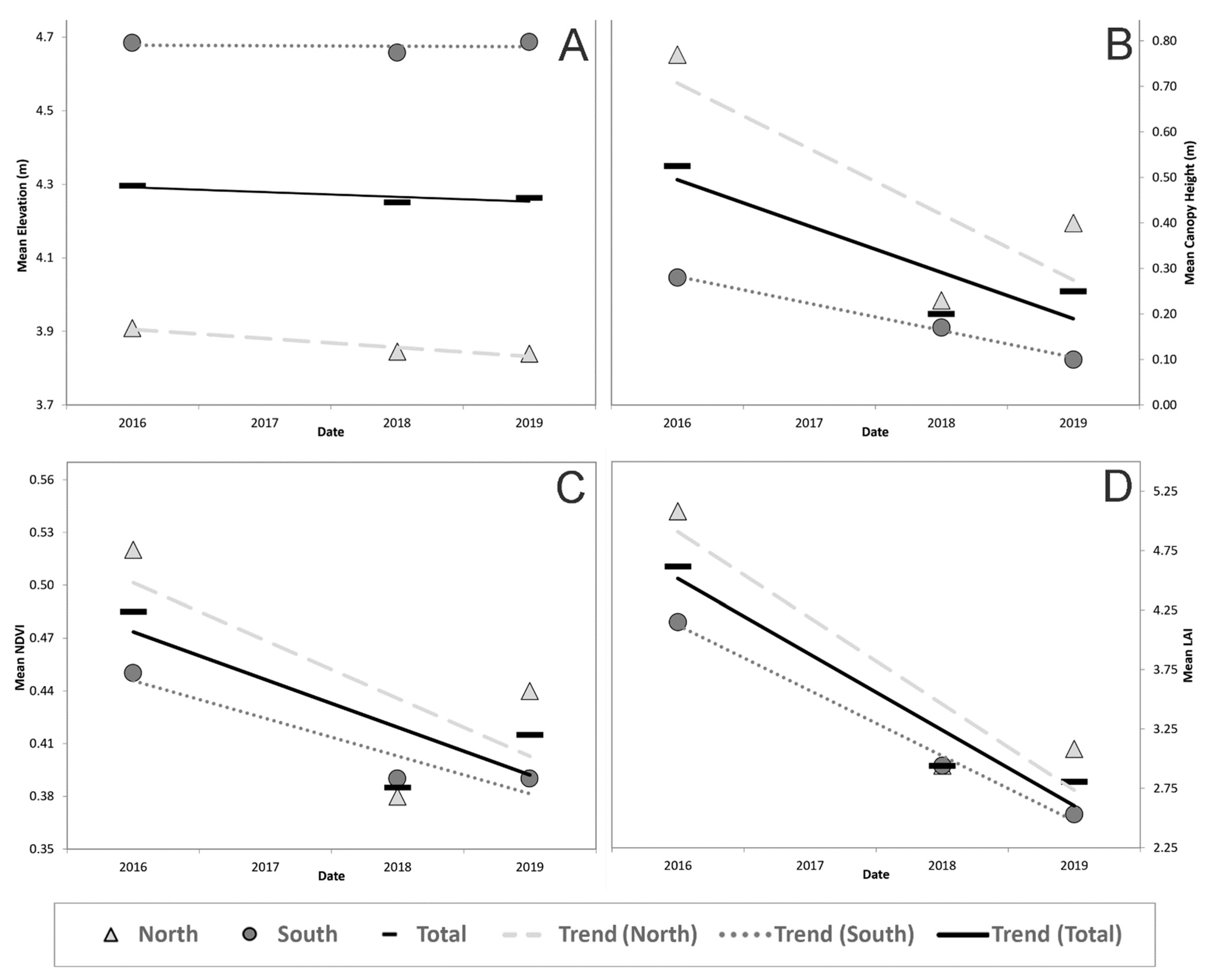
The Pea Island North and South AOIs had Low and Moderate overwash events, respectively. Table 5 provides the overwash designation, along with vegetation metric summary statistics (i.e., means and standard deviations) for Total Area, Vegetation Cover (VC), CHM, NDVI, and LAI, all derived from the DuneVeg Toolbox for the North and South assessment units. Similarly, Figure 3 provides the means and trends of DEM (A), CHM (B), NDVI (C), and LAI (D) values for the Pea Island units. These represent all qualifying data, from late-growing season, across the period of record (2016 to 2019).
The total area for the Pea Island North and South AOIs were 0.47 km2 and 0.27 km2, respectively (Table 5). The percentage of each AOI that was vegetated at any time ranged from a minimum of 10.52% (North AOI in 2016) to a maximum of 57.36% (North AOI in 2018). NOAA’s C-CAP land cover data show the vegetation in 2016 consisted of 84% emergent and 16% shrub in the North AOI, and 95% emergent and 5% shrub in the South AOI [55]. The summary statistics show all AOIs experienced similar vegetation cover trends, increasing significantly from 2016 to 2018, then experiencing smaller decreases between 2018 and 2019.
The elevation ranged from a low of 3.84 m to a high of 4.69 m (NAVD88), for the North AOI (2016) and South AOI (2019), respectively (Table 5 and Figure 3A). While the mean elevation in the South AOI remained relatively unchanged from 2016 through 2019, the North AOI experienced slight decreases in mean elevations, across the period of analysis. The total mean elevation for the Pea Island site (across all AOIs) remained relatively unchanged from year-to-year, decreasing from 4.29 m in 2016 to 4.25 m 2018, then increasing slightly to 4.26 m by 2019 (Figure 3A). Given the known overwash events within the AOIs, these mean elevations are indicative of sediment that was either reworked within the system or moved out of the system and replaced by sediment introduced via wind and tidal forces.
The range of CHM values for Pea Island was 0.1 m to 20 m. The mean CHM values ranged from a low of 0.12 m for the South AOI in 2019 to a high of 0.77 m for the North AOI in 2016 (Table 5 and Figure 3B). The North and South AOIs both experienced decreasing trends in CHM values across the entire period of analysis (2016 to 2019). The initial loss was driven largely by a reduction in canopy height in the North AOI, which experienced a −0.54 m reduction in mean CHM from 2016 to 2018. The North AOI did experience a minimal increase in mean CHM values from 2018 to 2019, while the South AOI experienced decreases across both time periods (2016–2018 and 2018–2019) (Figure 3B). All AOI-specific mean CHM values were significantly different between years (Tukey’s HSD [honestly significant difference]: p < 0.01).
Individual NDVI values (pixel-wise) ranged from 0 to 1 across all vegetated areas within the Pea Island study site, where low and high values were related to lower and higher levels of vegetation greenness (for vegetated areas), respectively. The mean NDVI values ranged from a low of 0.37 for the North AOI in 2018 to a high of 0.52 for the same AOI in 2016 (Table 5 and Figure 3C). The Pea Island sites experienced significant decreases in mean NDVI values between 2016 and 2018, decreasing from 0.52 to 0.37 and 0.45 to 0.39 for the North and South AOIs, respectfully (Figure 3C). While the North AOI did experience a moderate increase (recovery) in NDVI by 2019, the South AOI underwent a nominal decrease. By comparison, the decade (2006 to 2015) preceding this period of analysis (2016 to 2019) encountered larger but less frequent storms (Hurricane Irene, 2011; 25.9 ms−1 sustained winds and 2.35 m surge) and experienced moderately increasing NDVI trends (based on Landsat-derived NDVI data for the Pea Island study site). This is corroborated by previous studies which have shown vegetation typically recovers by the next full growing season after a major disturbance event [58].
The range of pixel-wise LAI values was 0 to ~10 (m2/m2) for the dune vegetation across all AOIs, where higher values were related to higher leaf area. Mean LAI values ranged from a low of 2.53 for the South AOI in 2019 to a high of 5.07 for the North AOI in 2016. The mean total LAI values for the Pea Island study site decreased from 4.38 in 2016, to 3.44 in 2018, to 3.09 in 2019 (Figure 3D). LAI experienced similar overall trends to those of CHM and NDVI, however, there was much smaller increase (recovery) in LAI in the North AOI in 2019, as compared to CHM and NDVI.
3.2. Multi-Temporal Trend Analysis
3.2.1. Elevation and Vegetation Metrics
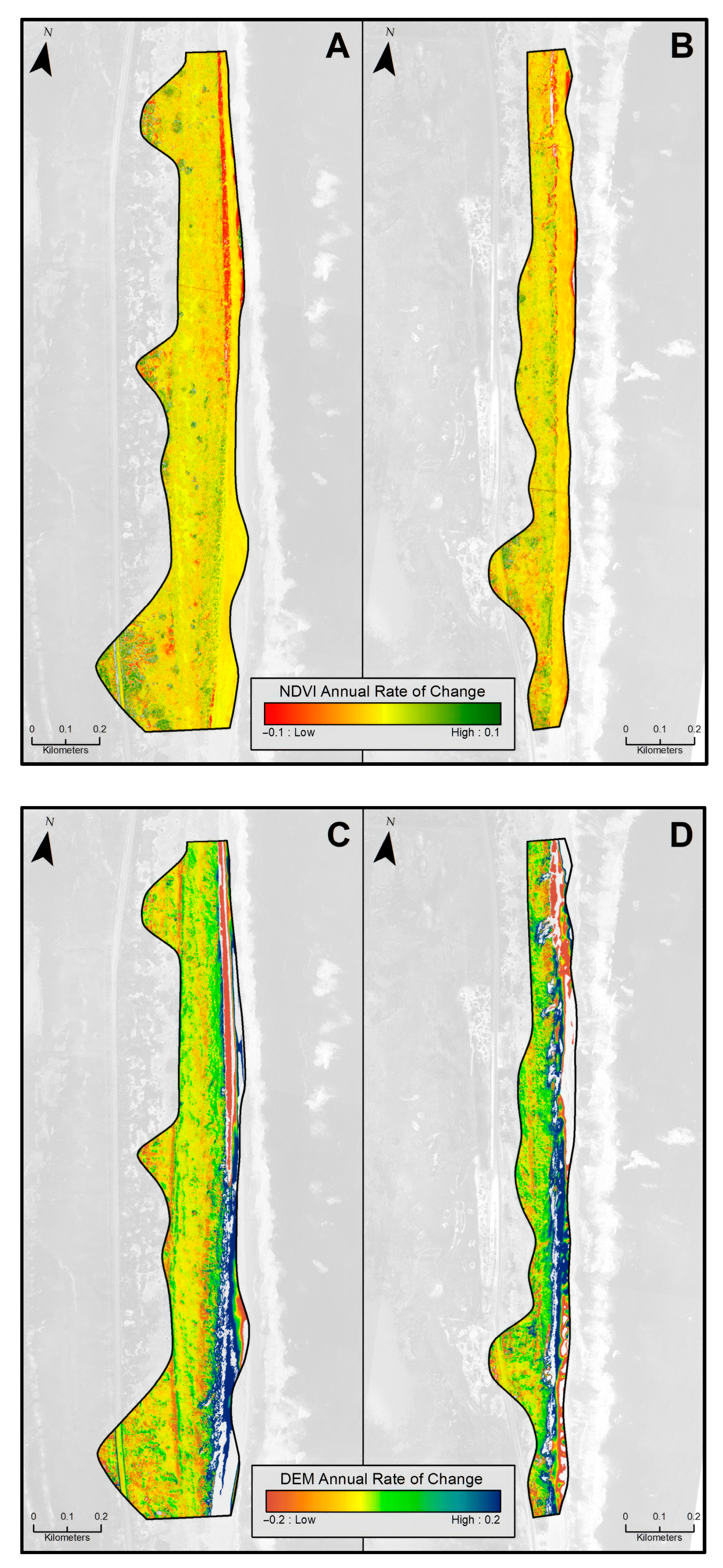
Although mean elevation and vegetation attribute values can provide general measures of wetland disturbance and recovery, they can also lack the detail required to evaluate the spatial variability and patterns associated with short- and long-term stressors. Data derived from the DuneVeg Toolbox were used in conjunction with the Curve Fit tool to evaluate changes in elevation and vegetation over space (across areas of low and moderate hurricane impacts) and time (across the period of analysis). Figure 4 provides examples of the rate of change and spatial variability of elevation (Panels A, B) and vegetation productivity (Panels C, D), on a pixel-by-pixel basis. For the Northern AOI (Figure 4A), most elevation changes occurred oceanside along the beach and dune toe, with linear erosion along the northern beach (orange and red colors in Figure 4A) and sediment deposition in the central and southern portions (blue color in Figure 4A) of the AOI. The erosion in the Southern AOI was non-linear and indicative of sediment erosion and distribution induced by an overwash event. This is evidenced by the fragmented areas of erosion (orange and red in Figure 4B) throughout the northern and southern dunes in the Southern AOI. The central region of the South AOI was not overwashed and therefore experienced increasing rates of elevation (greens and blue in Figure 4B) as a result of sediment transport and deposition. The overwash events within the Southern AOI resulted in higher rates of accretion along the inter- and back-dunes (green color in Figure 4B) due to sediment transport beyond the primary dune.
Figure 4 also illustrates the vegetation biomass (NDVI) rates of change and spatial patterns on a per-pixel basis within the Pea Island AOIs. The NDVI rates of change are color-ramped (Figure 4, Panels C and D), where the orange-to-red colors represent decreasing rates of NDVI, and the yellow-to-green colors represent increasing rates. The Pea Island North AOI (Panel C) and South AOI (Panel D) encountered similar patterns of change, with the majority of each unit experiencing slight decreasing rates of NDVI (represented by a light orange color), while smaller regions experienced higher decreasing (linear features to the north, represented by darker shades of red) and higher increasing (disaggregated regions to the south, represented by darker shades of green) rates of NDVI. The areas of distinct decreasing NDVI were primarily along the beach and foredune features in each AOI while the areas of increasing NDVI occurred primarily at leeward positions within inter- or along secondary-dune features (Figure 4C,D). These change rates are consistent with the NDVI summary statistics for Pea Island, which showed an overall decreasing trend in NDVI within the period of analysis (Table 5 and Figure 3). The vegetation-based regression data (Figure 4C,D) correspond to the elevation data (Figure 4A,B), where areas of distinct reductions in NDVI (along dune features) coincide with distinct reductions in elevation. Likewise, areas with moderate increasing NDVI (interdune features) coincide with areas that experienced moderate elevation increases. The areas of distinct reductions are indicative of direct hurricane impacts (caused by wind and wave energies) in barrier island systems. The areas of increasing NDVI are indicative of indirect hurricane impacts in wetland systems, where overwashed sediments can result in elevation benefits, including flood stress reduction, and increases in productivity and aboveground biomass [59]. Similar trend analysis results were observed with LAI and CHM data, and are therefore not presented here, for brevity.
3.2.2. Hot Spot Analysis: Vegetation Metrics
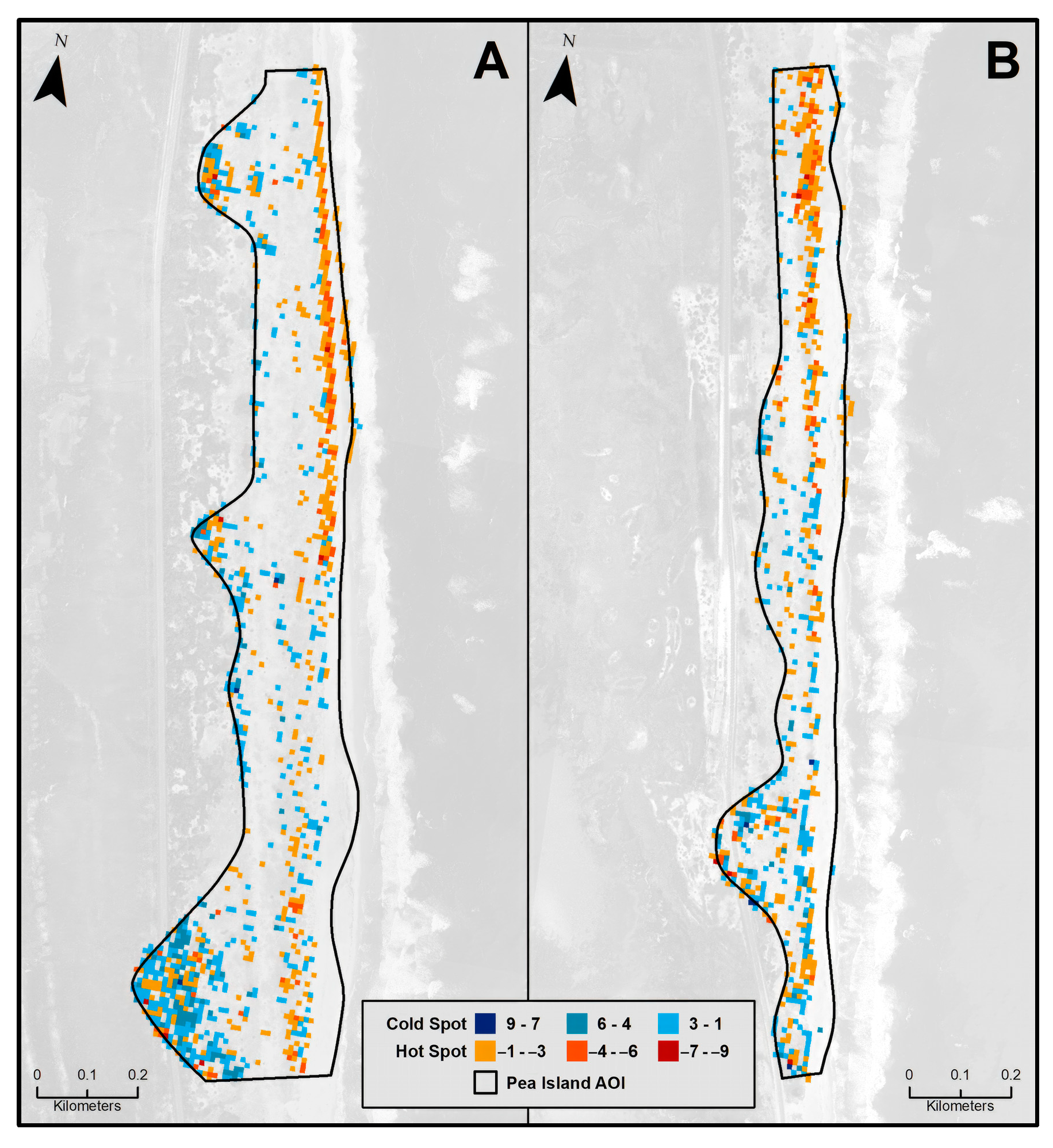
The Getis–Ord Gi* hot spot analysis was performed for each vegetation metric (CHM, LAI, NDVI). This process identifies pixels with significant values and assigns them to associated Gi* bins based on p-value confidence levels (Table 6). Bins for single metric analyses are determined at the p < 0.05, 0.01, and 0.001 levels, and assigned values of 1, 2, 3, and −1, −2, −3, for the Cold and Hot Spots, respectively. To perform a more comprehensive evaluation of vegetation change, the output layers from each individual hot spot analysis (CHM, LAI, and NDVI) were overlayed (summed) to provide a more robust vegetation hot spot assessment. This combined approach resulted in Gi* bins that ranged from 1 to 9 and −1 to −9, for cold and hot spots, respectively. Table 6 shows the results of the Getis–Ord Gi* hot spot analyses. Single metric assessments show only small portions of each AOI were classified as hot or cold spots, with a majority of those occurring at the p < 0.001 designations (3 and −3). For the multi-metric assessment, most of the hot and cold spot regions occurred at the p < 0.05 designation. This indicates most pixels that experienced significant vegetation-based rates of change either experienced those at the p < 0.001 level for only one vegetation metric, or at the p < 0.01 and/or 0.05 levels for multiple metrics.
Figure 5 shows the overall vegetation hot spot analysis, where the hot spot bins are represented by light orange (−1, −2, −3), dark orange (−4, −5, −6), and dark red (−7, −8, −9), respectively; while the cold spot bins are represented by light green (1, 2, 3), medium green (4, 5, 6), and dark green (7, 8, 9), respectively. Most of the hot spot areas (orange and red pixels, Figure 5) are concentrated within linear features at the northern reach of each Pea Island AOI or scattered throughout the southern portions of the AOIs. These hot spot areas represent regions within Pea Island where vegetation biomass and health experienced significant reductions across the entire period of analysis (2016 to 2019). The cold spot areas (Figure 5, blue pixels), which represent regions where vegetation biomass and health experienced significant increases across the period of analysis, are found primarily leeward of the primary dune along southern portions of the AOIs, or intermittently scattered throughout central portions of the AOIs.
4. Discussion
Dune vegetation plays a crucial role in the processes that control erosion, dune stability, and overall coastal resilience. Therefore, it is important for coastal managers to rapidly and accurately evaluate coastal vegetation properties and dynamics, especially in the face of current and future climate change trends. However, collecting or generating vegetation data that are useful for ecosystem management, or as inputs to coastal numerical models, can be challenging in coastal and island systems. Even when traditional data collections or monitoring techniques can be applied, they often lack the detail (i.e., spatial and temporal) or coverage required to evaluate finer scale changes, especially in complex and dynamic landscapes. This research effort demonstrated the use of DuneVeg Tool generated elevation and vegetation metric data to assess hurricane-induced trends and changes in coastal morphology and habitat. Summary statistics were shown to provide general elevation and vegetation trends across the period of analysis, but per-pixel regression and hot spot analyses provide the spatial detail necessary for assessing areas or features of concern. Although the period of analysis used to demonstrate the utility of the developed tools and metrics is relatively short (evaluating short-term and direct impacts from hurricanes), the application should be equally useful in assessing indirect impacts over longer time periods.
The DuneVeg tools and metrics may likewise prove useful in coastal numerical modeling. Models rely greatly on estimates of vegetation properties [60]. For instance, wave attenuation through vegetation is a highly variable function of not only hydrodynamics, but also of general vegetation characteristics. Recent studies have updated models that account for wave interactions using spatially explicit and variable vegetation characteristics as inputs [12]. However, model input data are limited, particularly for large scale or regional coastal projects, and therefore many models currently incorporate synthetic vegetation data or constant values as inputs. The vegetation data gaps that exist for many coastal numerical models could be narrowed by way of the vegetation metrics generated through the DuneVeg Tool. Future studies should evaluate the use of these vegetation metrics to refine numerical models and quantify the performance and accuracy of those models relative to existing data model inputs.
5. Conclusions
This study advances existing dune and coastal wetland system knowledge involving remote sensing techniques for classifying, quantifying, and estimating elevation and critical dune vegetation metrics. It also describes the use of summary statistics and regression analyses to evaluate spatial and temporal changes in vegetation properties. Future studies should evaluate the ability of the derived methods and metrics to quantify and monitor long-term indirect changes in coastal wetland vegetation. Future assessments should also investigate the power of fusing DuneVeg Toolbox data (combining geomorphology and environmental characteristics) for a holistic analysis paradigm (as opposed to individual assessments). The ability to combine and analyze spectral and LiDAR data together opens possibilities to explore landscapes as mosaics [61,62]. Still, the methodology and products derived as part of this study can aid researchers and managers in improving predictions of future disturbance, which would help in the advancement of coastal wetland monitoring, restoration, and adaptive management.
Author Contributions
Conceptualization, G.M.S., S.J. and M.R.; methodology, G.M.S. and S.J.; software, C.S.; validation, G.M.S. and S.J.; formal analysis, G.M.S.; investigation, G.M.S. and S.J.; data curation, M.R.; writing—original draft preparation, G.M.S. and S.J.; writing—review and editing, G.M.S., S.J., C.S. and M.R.; visualization, G.M.S.; supervision, G.M.S. and S.J.; project administration, M.R.; funding acquisition, M.R. All authors have read and agreed to the published version of the manuscript.
Funding
This research was funded by the U.S. Army Corps of Engineers, Engineer Research and Development Center’s Joint Airborne LiDAR Bathymetry Technical Center of Expertise (JALBTCX), Kiln, MS, USA and the National Coastal Mapping Program (NCMP), Mobile, AL, USA.
Data Availability Statement
Publicly available National Coastal Mapping Data are accessible at the National Oceanic and Atmospheric Administration (NOAA) Digital Coast website: https://coast.noaa.gov/digitalcoast/, accessed on 16 March 2020.
Acknowledgments
The authors would like to thank Jennifer Wozencraft, JALBTCX Director and NCMP Program Manager, for her support in authorizing and funding this work unit.
Conflicts of Interest
The authors declare no conflict of interest. The funders had no role in the design of the study; in the analyses, or interpretation of data; in the writing of the manuscript, or in the decision to publish the results.
References
- Charbonneau, B.R.; Wnek, J.P.; Langley, J.A.; Lee, G.; Balsamo, R.A. Above vs. belowground plant biomass along a barrier island: Implications for dune stabilization. J. Environ. Manag. 2016, 182, 126–133. [Google Scholar] [CrossRef]
- Michener, W.K.; Blood, E.R.; Bildstein, K.L.; Brinson, M.M.; Gardner, L.R. Climate change, hurricanes and tropical storms, and rising sea level in coastal wetlands. Ecol. Appl. 1997, 7, 770–801. [Google Scholar] [CrossRef]
- Robin, N.; Billy, J.; Castelle, B.; Hesp, P.; Nicolae Lerma, A.; Laporte-Fauret, Q.; Marieu, V.; Rosebery, D.; Bujan, S.; Destribats, B.; et al. 150 Years of foredune initiation and evolution driven by human and natural processes. Geomorphology 2021, 374, 107516. [Google Scholar] [CrossRef]
- U.S. Army Corps of Engineers (USACE). Hurricane Sandy Coastal Projects Performance Evaluation Study: Disaster Relief Appropriations Act 2013; U.S. Army Corps of Engineers, Report submitted to Congress by the Assistant Secretary of the Arm for Civil Works; American Shore and Beach Preservation Association: Redondo Beach, CA, USA, 2013; p. 106. [Google Scholar]
- Wigand, C.; Ardito, T.; Chaffee, C.; Ferguson, W.; Paton, S.; Raposa, K.; Vandemoer, C.; Watson, E. A climate change adaptation strategy for management of coastal marsh systems. Estuaries Coasts 2017, 40, 682–693. [Google Scholar] [CrossRef] [PubMed]
- Sigren, J.M.; Figlus, J.; Armitage, A.R. Coastal sand dunes and dune vegetation: Restoration, erosion, and storm protection. Shore Beach 2014, 82, 5–12. [Google Scholar]
- Suir, G.M.; Sasser, C.E.; Harris, J.M. Use of Remote Sensing and Field Data to Quantify the Performance and Resilience of Restored Louisiana Wetlands. Wetlands 2020, 40, 2643–2658. [Google Scholar] [CrossRef]
- Klemas, V. Remote sensing of coastal wetland biomass: An overview. J. Coast. Res. 2013, 29, 1016–1028. [Google Scholar] [CrossRef]
- Davies, J.L. Geographical Variation in Coastal Development, 2nd ed.; Longman: London, UK, 1980; p. 212. [Google Scholar]
- Board, O.S. Understanding the Long-Term Evolution of the Coupled Natural-Human Coastal System: The Future of the US Gulf Coast; National Academies Press: Washington, DC, USA, 2018; p. 156. [Google Scholar] [CrossRef]
- Suir, G.M.; Sasser, C.E. Redistribution and impacts of nearshore berm sediments on the Chandeleur barrier islands, Louisiana. Ocean. Coast. Manag. 2019, 168, 103–116. [Google Scholar] [CrossRef]
- Anderson, M.E.; Smith, J.M.; Bryant, D.B.; McComas, R.W. Laboratory Studies of Wave Attenuation through Artificial and Real Vegetation; ERDC TR-13-11; U.S. Army Corps of Engineers: Washington, DC, USA, 2013; p. 93. [Google Scholar]
- Shuman, C.S.; Ambrose, R.F. A comparison of remote sensing and ground-based methods for monitoring wetland restoration success. Restor. Ecol. 2003, 11, 325–333. [Google Scholar] [CrossRef]
- Rosette, J.; Suárez, J.; Nelson, R.; Los, S.; Cook, B.; North, P. Lidar remote sensing for biomass assessment. In Remote Sensing of Biomass-Principles and Applications; Fatoyinbo, T., Ed.; InTech: Rijeka, Croatia, 2012; p. 322. [Google Scholar]
- Deo, R.K.; Russell, M.B.; Domke, G.M.; Woodall, C.W.; Falkowski, M.J.; Cohen, W.B. Using Landsat time-series and LiDAR to inform aboveground forest biomass baselines in northern Minnesota, USA. Can. J. Remote Sens. 2017, 43, 28–47. [Google Scholar] [CrossRef]
- Wang, J.; Liu, Z.; Yu, H.; Li, F. Mapping Spartina alterniflora Biomass Using LiDAR and Hyperspectral Data. Remote Sens. 2017, 9, 589. [Google Scholar] [CrossRef]
- Luo, S.; Wang, C.; Xi, X.; Pan, F.; Qian, M.; Peng, D.; Nie, S.; Qin, H.; Lin, Y. Retrieving aboveground biomass of wetland Phragmites australis (common reed) using a combination of airborne discrete-return LiDAR and hyperspectral data. Int. J. Appl. Earth Obs. Geoinf. 2017, 58, 107–117. [Google Scholar] [CrossRef]
- Luo, S.; Wang, C.; Xi, X.; Pan, F.; Peng, D.; Zou, J.; Nie, S.; Qin, H. Fusion of airborne LiDAR data and hyperspectral imagery for aboveground and belowground forest biomass estimation. Ecol. Indic. 2017, 73, 378–387. [Google Scholar] [CrossRef]
- Jaber, R.; Florence, M.; Brilli, N.; Paprocki, J.; Popelka, J.; Stark, N. Geotechnical Investigation of the Intertidal Zone in Duck, North Carolina, during Tropical Storm Melissa and DUNEX. In Proceedings of the American Geophysical Union Meeting on Ocean Sciences, San Diego, CA, USA, 16–21 February 2020. [Google Scholar]
- Bork, B.W.; West, N.E.; Price, K.P. Calibration of broad- and narrow-band spectral variables for rangeland cover component quantification. Int. J. Remote Sens. 1999, 20, 3641–3662. [Google Scholar] [CrossRef]
- Cialone, M.; Elko, N.; Lillycrop, J.; Stockdon, H.; Raubenheimer, B.; Rosati, J. During Nearshore Event Experiment (DUNEX): A Collaborative Community Field Data Collection Effort. In Proceedings of the 9th International Conference on Coastal Sediments, Tampa, FL, USA, 27–31 May 2019; pp. 2958–2966. [Google Scholar] [CrossRef]
- Rey, A.J.; Mulligan, R.P. Influence of Hurricane Wind Field Variability on Real-time Forecast Simulations of the Coastal Environment. J. Geophys. Res. Ocean. 2021, 126, e2020JC016489. [Google Scholar] [CrossRef]
- National Oceanic and Atmospheric Administration (NOAA). National Weather Service Event Summaries and Case Studies: Newort/Morehead City, North Carolina. Available online: https://www.weather.gov/mhx/SignificantEvents (accessed on 21 May 2021).
- Kiln, M.S.; U.S. Army Corps of Engineers (USACE). Joint Airborne LiDAR Bathymetry Technical Center of Expertise (JALBTCX). 2020. Available online: www.sam.usace.army.mil/Missions/Spatial-Data-Branch/JALBTCX (accessed on 16 March 2020).
- Schowengerdt, R.A. Remote Sensing: Models and Methods for Image Processing, 3rd ed.; Academic Press: Cambridge, MA, USA; Elsevier: Burlington, MA, USA, 2007; p. 515. [Google Scholar]
- Park, J.Y.; Tuell, G. Conceptual design of the CZMIL data processing system (DPS): Algorithms and software for fusing lidar, hyperspectral data, and digital images. In Proceedings of the Society of Photo-optical Instrumentation Engineers Conference on Algorithms and Technologies for Multispectral, Hyperspectral, and Ultraspectral Imagery XVI, 769510, Orlando, FL, USA, 5–9 April 2010. [Google Scholar] [CrossRef]
- Wozencraft, J.; Dunkin, L.; Eisemann, E.; Reif, M. Chapter 7: Applications, Ancillary Systems, and Fusion. In Airborne Laser Hydrography II; Philpot, W., Ed.; eCommons: Ithaca, NY, USA, 2019; pp. 207–230. [Google Scholar]
- Reif, M.K.; Krumwiede, B.S.; Brown, S.E.; Theuerkauf, E.J.; Harwood, J.H. Nearshore Benthic Mapping in the Great Lakes: A Multi-Agency Data Integration Approach in Southwest Lake Michigan. Remote Sens. 2021, 13, 3026. [Google Scholar] [CrossRef]
- Wozencraft, J.M.; Lillycrop, W.J. JALBTCX coastal mapping for the USACE. Int. Hydrogr. Rev. 2006, 7, 28–37. [Google Scholar]
- Malone, K.; Williams, H. Growing Season Definition and Use in Wetland Delineation; ERDC/CRREL CR-10-3; U.S. Army Corps of Engineers: Washington, DC, USA, 2010; p. 48. [Google Scholar]
- Jackson, S.S.; Saltus, C.L.; Reif, M.K.; Suir, G.M. During Nearshore Event Vegetation Gradation (DUNEVEG): Geospatial Tools for Automating Remote Vegetation Extraction; ERDC/EL SR-23-X; U.S. Army Corps of Engineers, Engineer Research and Development Center: Washington, DC, USA, 2023; Special Report; in press. [Google Scholar]
- Suir, G.M.; Sasser, C.E. Use of NDVI and landscape metrics to assess effects of riverine inputs on wetland productivity and stability. Wetlands 2019, 39, 815–830. [Google Scholar] [CrossRef]
- Suir, G.M.; Saltus, C.L.; Reif, M.K. Geospatial Assessments of Phragmites australis Die-Off in South Louisiana: Preliminary Findings; ERDC/EL TR-18-9; U.S. Army Engineer Research and Development Center: Vicksburg, MS, USA, 2018. [Google Scholar]
- Weier, J.; Herring, D. Measuring Vegetation: NDVI and EVI. NASA Earth Observatory. 2000. Available online: https://earthobservatory.nasa.gov/features/MeasuringVegetation/measuring_vegetation_2.php (accessed on 15 March 2023).
- Lan, Y.; Zhang, H.; Lacey, R.; Hoffmann, W.C.; Wu, W. Development of an integrated sensor and instrumentation system for measuring crop conditions. Agric. Eng. J. 2009, 11, 11–15. [Google Scholar]
- Myneni, R.B.; Hall, F.G.; Sellers, P.J.; Marshak, A.L. The interpretation of spectral vegetation indexes. IEEE Trans. Geosci. Remote Sens. 1995, 33, 481–486. [Google Scholar] [CrossRef]
- Yang, Y.; Zhu, J.; Zhao, C.; Liu Tong, S. The spatial continuity study of NDVI based on Kriging and BPNN algorithm. J. Math. Comput. Model. 2011, 54, 1138–1144. [Google Scholar] [CrossRef]
- Rouse, J.W.; Haas, R.H.; Scheel, J.A.; Deering, D.W. Monitoring Vegetation Systems in the Great Plains with ERTS. In Proceedings of the 3rd Earth Resource Technology Satellite (ERTS) Symposium, Washington, DC, USA, 10–14 December 1973. [Google Scholar]
- Lillesand, T.M.; Kiefer, R.W.; Chipman, J.W. Remote Sensing and Image Interpretation, 5th ed.; John Wiley and Sons: New York, NY, USA, 2004; p. 763. [Google Scholar]
- Moreau, S.; Bossenob, R.; Xing, F.G.; Baret, F. Assessing the biomass dynamics of Andean bofedal and totora high-protein wetland grasses from NOAA/AVHRR. Remote Sens. Environ. 2003, 85, 516–529. [Google Scholar] [CrossRef]
- Fang, H.; Liang, S. Leaf area index models. In Encyclopedia of Ecology; Jørgensen, S.E., Fath, B.D., Eds.; Elsevier: Amsterdam, The Netherlands, 2008; pp. 2139–2148. [Google Scholar] [CrossRef]
- O’Connell, J.L.; Byrd, K.B.; Kelly, M. A Hybrid Model for Mapping Relative Differences in Belowground Biomass and Root:Shoot Ratios Using Spectral Reflectance, Foliar N and Plant Biophysical Data within Coastal Marsh. Remote Sens. J. 2015, 7, 16480–16503. [Google Scholar] [CrossRef]
- Boegh, E.; Soegaard, H.; Broge, N.; Hasager, C.B.; Jensen, N.O.; Schelde, K.; Thomsen, A. Airborne multispectral data for quantifying leaf area index, nitrogen concentration, and photosynthetic efficiency in agriculture. Remote Sens. Environ. 2002, 81, 179–193. [Google Scholar]
- Huete, A.; Didan, K.; Miura, T.; Rodriguez, E.P.; Gao, X.; Ferreira, L.G. Overview of the radiometric and biophysical performance of the MODIS vegetation indices. Remote Sens. Environ. 2002, 83, 195–213. [Google Scholar] [CrossRef]
- Huete, A.R.; Justice, C.; van Leeuwen, W. MODIS Vegetation Index (MOD13): Algorithm Theoretical Basis Document; University of Arizona, Vegetation Index and Phenology Lab: Tucson, AZ, USA, 1999; Volume 3, pp. 295–309. [Google Scholar]
- Gremillion, S.; Wallace, D.; Eisemann, E.; Culver-Miller, E.; Funderburk, W. Washover Volume Analysis of Hatteras and Pea Islands, North Carolina, USA over Centennial Timescales. Authorea Prepr. 2022. [Google Scholar] [CrossRef]
- ASPRS. ASPRS Accuracy Standards for Digital Geospatial Data. 2015. Available online: http://www.asprs.org/a/society/divisions/pad/Accuracy/Draft_ASPRS_Accuracy_Standards_for_Digital_Geospatial_Data_PE&RS.pdf (accessed on 16 July 2022).
- Doran, K.J.; Sallenger, A.H.; Reynolds, B.J.; Wright, C. Accuracy of EAARL Lidar Ground Elevations Using a Bare-Earth Algorithm in Marsh and Beach Grasses on the Chandeleur Islands, Louisiana; U.S. Geological Survey OpenFile Report 2010–1163; USGS Science for a Changing World: Washington, DC, USA, 2010; 9p. [Google Scholar]
- Wang, C.; Menenti, M.; Stoll, M.P.; Feola, A.; Belluco, E.; Marani, M. Separation of Ground and Low Vegetation Signatures in LiDAR Measurements of Salt-Marsh Environments. IEEE Trans. Geosci. Remote Sens. 2009, 47, 2014–2023. [Google Scholar] [CrossRef]
- Hladik, C.; Alber, M. Accuracy assessment and correction of a LIDAR-derived salt marsh digital elevation model. Remote Sens. Environ. 2012, 121, 224–235. [Google Scholar] [CrossRef]
- Populus, J.; Barreau, G.; Fazilleau, J.; Kerdreux, M.; L’Yavanc, J. Assessment of the LIDAR topographic technique over a coastal area. In Proceedings of the CoastGIS’01: 4th International Symposium on GIS and Computer Mapping for Coastal Zone Management, Halifax, NS, Canada, 18–20 June 2001. [Google Scholar]
- Rau, G.; Shih, Y.S. Evaluation of Cohen’s kappa and other measures of inter-rater agreement for genre analysis and other nominal data. J. Engl. Acad. Purp. 2021, 53, 101026. [Google Scholar] [CrossRef]
- Wang, P.; Briggs, T.M.R. 2015. Storm-Induced morphology changes along barrier islands and poststorm recovery. In Coastal and Marine Hazards, Risks, and Disasters; Elsevier: Amsterdam, The Netherlands, 2015; pp. 271–306. [Google Scholar]
- De Jager, N.R.; Fox, T.J. Curve Fit: A pixel-level raster regression tool for mapping spatial patterns. Methods Ecol. Evol. 2013, 4, 789–792. [Google Scholar] [CrossRef]
- Office for Coastal Management. NOAA’s Coastal Change Analysis Program (C-CAP) 2016 Regional Land Cover Data—Coastal United States from 2010-06-15 to 2010-08-15. NOAA National Centers for Environmental Information. 2022. Available online: https://www.fisheries.noaa.gov/inport/item/48336 (accessed on 15 March 2023).
- Meredith, A.W.; Krabill, W.B.; List, J.H.; Reiss, T.E.; Frederick, E.B. An Assessment of NASA’s Airborne Topographic Mapper Instrument for Beach Topographic Mapping at Duck, North Carolina; Coastal Services Center Technical Report CSC/9-98/001 Version 1.0; National Oceanic and Atmospheric Administration, Coastal Services Center: Charleston, SC, USA, 1998. [Google Scholar]
- Schmid, K.A.; Hadley, B.C.; Wijekoon, N. Vertical accuracy and use of topographic LIDAR data in coastal marshes. J. Coast. Res. 2011, 27, 116–132. [Google Scholar] [CrossRef]
- Suir, G.M.; Saltus, C.L.; Reif, M.K. Remote sensing-based structural and functional assessments of Phragmites australis diebacks in the Mississippi River Delta. Ecol. Indic. 2022, 135, 108549. [Google Scholar] [CrossRef]
- Walters, D.C.; Kirwan, M.L. Optimal hurricane overwash thickness for maximizing marsh resilience to sea level rise. Ecol. Evol. 2016, 6, 2948–2956. [Google Scholar] [CrossRef] [PubMed]
- Smith, J.M.; Bryant, M.A.; Wamsley, T.V. Wetland buffers: Numerical modeling of wave dissipation by vegetation. Earth Surf. Process. Landf. 2016, 41, 847–854. [Google Scholar] [CrossRef]
- Judah, A.; Hu, B. An Advanced Data Fusion Method to Improve Wetland Classification Using Multi-Source Remotely Sensed Data. Sensors 2022, 22, 8942. [Google Scholar] [CrossRef] [PubMed]
- Kahraman, S.; Bacher, R. A comprehensive review of hyperspectral data fusion with lidar and sar data. Annu. Rev. Control. 2021, 51, 236–253. [Google Scholar] [CrossRef]
Figure 1.
Location map of Pea Island study site and assessment units (areas of interest).

Figure 2.
Example of the hyperspectral imagery (A), digital elevation model (B), canopy height model (C), normalized difference vegetation index (D), vegetation density (E), and leaf area index (F) within the Pea Island South assessment area.
Figure 2.
Example of the hyperspectral imagery (A), digital elevation model (B), canopy height model (C), normalized difference vegetation index (D), vegetation density (E), and leaf area index (F) within the Pea Island South assessment area.

Figure 3.
Means and trends of digital elevation model (A), canopy height model (B), normalized difference vegetation index (C), and leaf area index (D) within Pea Island assessment units from 2016 to 2019.
Figure 3.
Means and trends of digital elevation model (A), canopy height model (B), normalized difference vegetation index (C), and leaf area index (D) within Pea Island assessment units from 2016 to 2019.

Figure 4.
Elevation and normalized difference vegetation index regression (per-pixel rate of change from 2016 to 2019) within the Pea Island North (A,C) and Pea Island South (B,D) assessment units.
Figure 4.
Elevation and normalized difference vegetation index regression (per-pixel rate of change from 2016 to 2019) within the Pea Island North (A,C) and Pea Island South (B,D) assessment units.

Figure 5.
Multi-metric (canopy height, leaf area, and normalized difference vegetation index) vegetation analysis using Getis–Ord Gi* statistics within the Pea Island North (A) and South (B) assessment units. Colors represent areas of statistically significantly high levels of decreasing (orange to red) and increasing (light to dark blue) vegetation.


Table 1.
Summary of CZMIL collection type, date, location and purpose in the North Carolina Outer Banks from 2016 to 2019.
Table 1.
Summary of CZMIL collection type, date, location and purpose in the North Carolina Outer Banks from 2016 to 2019.
| Data Type | Collection Date | Location | Purpose |
|---|---|---|---|
| Hyperspectral (1 m), LiDAR (1 m), RGB (5 cm) | 22 November 2016 | Pea Island, NC, USA | Post-hurricane Matthew |
| Hyperspectral (1 m), LiDAR (1 m), RGB (5 cm) | 15 October 2018 | Pea Island, NC, USA | Post-hurricane Florence |
| Hyperspectral (1 m), LiDAR (1 m), RGB (5 cm) | 1 October 2019 | DUNEX Extent | DUNEX |
Table 2.
Summary of dune vegetation metrics generated from the DuneVeg Toolbox used for conducting multi-temporal trend analysis. Included are National Coastal Mapping Program (NCMP) collection dates (year) used for each metric.
Table 2.
Summary of dune vegetation metrics generated from the DuneVeg Toolbox used for conducting multi-temporal trend analysis. Included are National Coastal Mapping Program (NCMP) collection dates (year) used for each metric.
| Metric | NCMP Data Product | NCMP Collection Year |
|---|---|---|
| Normalized Difference Vegetation Index (NDVI) | HSI | 2016, 2018, 2019 |
| Vegetation Cover (VC) | HSI | 2016, 2018, 2019 |
| Leaf Area Index (LAI) | HSI | 2016, 2018, 2019 |
| Digital Elevation Model (DEM) | LiDAR | 2016, 2018, 2019 |
| Digital Surface Model (DSM) | LiDAR | 2016, 2018, 2019 |
| Canopy Height Model (CHM) | LiDAR | 2016, 2018, 2019 |
Table 3.
Hurricanes that made landfall from 2016 to 2019 on or near the Pea Island study site.
| Hurricane | Date (Landfall) | Wind Speed (Landfall) | Maximum Surge |
|---|---|---|---|
| Hermine | 3 September 2016 | 20.6 ms−1 | 1.06 m |
| Matthew | 9 October 2016 | 21.9 ms−1 | 1.09 m |
| Florence | 14 September 2018 | 11.6 ms−1 | 0.90 m |
| Michael | 12 October 2018 | 23.2 ms−1 | 1.65 m |
| Dorian | 6 September 2019 | 20.1 ms−1 | 1.33 m |
Table 4.
Confusion matrix of vegetation classes derived from hyperspectral imagery.
| Observed | ||||||
|---|---|---|---|---|---|---|
| HIS Derived | Class | Sparse | Moderate | Dense | Total | User’s acc. |
| Sparse | 58 | 4 | 1 | 63 | 0.92 | |
| Moderate | 2 | 51 | 4 | 57 | 0.89 | |
| Dense | 0 | 5 | 55 | 60 | 0.92 | |
| Total | 60 | 60 | 60 | 180 | 0.00 | |
| Producer’s acc. | 0.97 | 0.85 | 0.92 | 0.00 | 0.87 | |
Table 5.
Raster-derived mean area (Total Area), vegetation cover (Veg Cover), elevation, canopy height (CHM), normalized difference vegetation index (NDVI), and leaf area index (LAI) within the Pea Island assessment units.
Table 5.
Raster-derived mean area (Total Area), vegetation cover (Veg Cover), elevation, canopy height (CHM), normalized difference vegetation index (NDVI), and leaf area index (LAI) within the Pea Island assessment units.
| Location | Overwash | Date | Total Area | Veg Cover | Elevation (m) | CHM (m) | NDVI | LAI (m2/m2) | ||||
|---|---|---|---|---|---|---|---|---|---|---|---|---|
| Km2 | Percent | Mean | Std | Mean | Std | Mean | Std | Mean | Std | |||
| North | Low | 2016 | 0.47 | 10.52 | 3.91 | 2.09 | 0.77 | 1.21 | 0.52 | 0.18 | 5.07 | 3.61 |
| North | Low | 2018 | 0.47 | 57.36 | 3.85 | 2.09 | 0.23 | 0.61 | 0.37 | 0.16 | 2.94 | 1.49 |
| North | Low | 2019 | 0.47 | 22.03 | 3.84 | 2.14 | 0.42 | 1.03 | 0.45 | 0.23 | 3.08 | 1.72 |
| South | Moderate | 2016 | 0.27 | 10.61 | 4.68 | 2.16 | 0.28 | 0.45 | 0.45 | 0.15 | 4.15 | 2.32 |
| South | Moderate | 2018 | 0.27 | 48.29 | 4.66 | 2.19 | 0.17 | 0.29 | 0.39 | 0.14 | 2.94 | 1.50 |
| South | Moderate | 2019 | 0.27 | 23.29 | 4.69 | 2.26 | 0.12 | 0.36 | 0.38 | 0.18 | 2.53 | 1.25 |
Table 6.
Hot spot analysis of vegetation metrics using the Getis–Ord Gi* and corresponding z-scores and p-values.
Table 6.
Hot spot analysis of vegetation metrics using the Getis–Ord Gi* and corresponding z-scores and p-values.
| Cluster Type | CHM | LAI | NDVI | Multi-Metric | Gi* Bin | Z-Score | p-Value | ||||
|---|---|---|---|---|---|---|---|---|---|---|---|
| Number | Area (ha) | Number | Area (ha) | Number | Area (ha) | Number | Area (ha) | (Single, Combined) | |||
| Hot Spot | 251 | 2.51 | 149 | 1.49 | 274 | 2.74 | 13 | 0.13 | (−3, −7–−9) | −4.97 | p < 0.001 |
| Hot Spot | 128 | 1.28 | 74 | 0.74 | 128 | 1.28 | 141 | 1.41 | (−2,− 4–−6) | −2.27 | p < 0.01 |
| Hot Spot | 97 | 0.97 | 62 | 0.62 | 119 | 1.19 | 778 | 7.78 | (−1, −1–−3) | −1.81 | p < 0.05 |
| Not Significant | 7167 | 71.67 | 7554 | 75.54 | 6629 | 66.29 | 6152 | 61.52 | (0, 0, 0) | 0.02 | |
| Cold Spot | 35 | 0.35 | 17 | 0.17 | 157 | 1.57 | 704 | 7.04 | (1, 1–3) | 1.81 | p < 0.05 |
| Cold Spot | 53 | 0.53 | 39 | 0.39 | 191 | 1.91 | 140 | 1.40 | (2, 4–6) | 2.26 | p < 0.01 |
| Cold Spot | 205 | 2.05 | 41 | 0.41 | 438 | 4.38 | 8 | 0.08 | (3, 7–9) | 5.73 | p < 0.001 |
Disclaimer/Publisher’s Note: The statements, opinions and data contained in all publications are solely those of the individual author(s) and contributor(s) and not of MDPI and/or the editor(s). MDPI and/or the editor(s) disclaim responsibility for any injury to people or property resulting from any ideas, methods, instructions or products referred to in the content. |
© 2023 by the authors. Licensee MDPI, Basel, Switzerland. This article is an open access article distributed under the terms and conditions of the Creative Commons Attribution (CC BY) license (https://creativecommons.org/licenses/by/4.0/).
Share and Cite
MDPI and ACS Style
Suir, G.M.; Jackson, S.; Saltus, C.; Reif, M. Multi-Temporal Trend Analysis of Coastal Vegetation Using Metrics Derived from Hyperspectral and LiDAR Data. Remote Sens. 2023, 15, 2098. https://doi.org/10.3390/rs15082098
AMA Style
Suir GM, Jackson S, Saltus C, Reif M. Multi-Temporal Trend Analysis of Coastal Vegetation Using Metrics Derived from Hyperspectral and LiDAR Data. Remote Sensing. 2023; 15(8):2098. https://doi.org/10.3390/rs15082098
Chicago/Turabian StyleSuir, Glenn M., Sam Jackson, Christina Saltus, and Molly Reif. 2023. "Multi-Temporal Trend Analysis of Coastal Vegetation Using Metrics Derived from Hyperspectral and LiDAR Data" Remote Sensing 15, no. 8: 2098. https://doi.org/10.3390/rs15082098
Note that from the first issue of 2016, this journal uses article numbers instead of page numbers. See further details here.