Enhanced Estimate of Chromophoric Dissolved Organic Matter Using Machine Learning Algorithms from Landsat-8 OLI Data in the Pearl River Estuary

Abstract

Chromophoric Dissolved Organic Matter (CDOM) plays a critical role in the carbon and biogeochemical cycles within aquatic ecosystems. Satellite imagery can be employed to determine aquatic CDOM concentrations, highlighting the need for effective and precise algorithms for this task. In this study, a cruise survey dataset containing CDOM absorption coefficients and water-leaving radiances in the Pearl River estuary (PRE) was utilized to develop machine learning algorithms for CDOM retrieval from Landsat-8 Operational Land Imager (OLI) observations. Based on OLI wavelength bands, five bands and six band-ratios were chosen as input parameters for the machine learning models. Six machine learning models were trained to develop CDOM algorithms, including Support Vector Regression (SVR), Random Forest (RF), Extreme Gradient Boosting (XGBoost), Multi-Layer Perceptron (MLP), and Convolutional Neural Network (CNN). The results indicated that, among the six machine learning models, the XGBoost algorithm performed best, with the highest R² value of 0.9 and the lowest CDOM root mean square error (RMSE) of 0.37 m⁻¹, outperforming empirical algorithms. The XGBoost algorithm identified B4/B1 as the most critical input parameter, contributing 71%, followed by B3/B2 with a 16% contribution, where B1, B2, B3, and B4 are the wavelength bands of the OLI. These two band-ratios accounted for most of the contributions, suggesting their significant role in CDOM retrieval from Landsat OLI images. By employing the developed XGBoost algorithm, CDOM spatial patterns at six instances were derived from Landsat-8 OLI image reflectance, illustrating CDOM variations in the PRE influenced by various factors. Further analysis revealed that, in the PRE, tides and winds are the primary driving forces behind the spatial and temporal variability of CDOM. At present, the exploration of employing machine learning algorithms to infer CDOM concentrations in this region remains relatively limited; therefore, with a higher R² value, the machine learning model we established unveils fresh and novel results.

1. Introduction

Widely distributed in all natural waters, Chromophoric Dissolved Organic Matter (CDOM) is a soluble and complex mixture of organic compounds [1]. The absorption spectra of CDOM under solar irradiation are mostly in the UV (250–400 nm) range and decrease exponentially with wavelength [2]. The presence of CDOM in aquatic environments can significantly impact the underwater light field, leading to a chain reaction of photochemical processes that, in turn, affect the biogeochemical cycling of vital elements such as carbon, nitrogen, and phosphorus. These photochemical reactions can alter the water’s optical properties and potentially disrupt the balance of its chemistry, which can have far-reaching impacts on the aquatic ecosystem. This highlights the crucial role that CDOM plays in shaping the health and functioning of water bodies, making it an important factor to consider in understanding and managing these vulnerable environments [3,4,5,6].

The aquatic CDOM comes from multiple sources [7,8] and can accelerate global warming through the emission of greenhouse gases such as carbon dioxide and methane [9]. Therefore, monitoring the CDOM in aquatic environments and understanding its response to environmental changes are of great significance. For large-scale monitoring of water quality, the high spatial variations of CDOM characteristics cannot be fully captured by observations from limited or sparse stations [10]. To solve this problem, remote sensing technology enables the rapid acquisition of water surface data and the measurement of CDOM concentrations with large-scale coverage at a low cost [11]. It has become an important method for implementing long-term and large-scale monitoring of eutrophication levels in water bodies [12].

For estimating CDOM from satellite imagery, the semi-analytic method and quasi-analytic algorithm (QAA) were introduced by Lee et al. [13], and an improved version was later developed [14]. Semi-analytic methods enhance the algorithm model by improving its generalizability and providing clear physical meaning to each parameter, resulting in increased accuracy and robustness. However, these semi-analytical methods depend on a complex theory of radiative transmission and require separating water columns’ optical compositions and determining their intrinsic optical properties accurately, making them difficult to use in coastal and inland water bodies that have complicated compositions and trophic states [15]. Some CDOM estimation algorithms are established empirically [16,17,18,19]. These methods are often based on simple linear, exponential, or logarithmic models derived from statistical relationships between the target parameters of the water system and the reflectance measured remotely. These models are used to calculate CDOM with different bands or band combinations based on linear or nonlinear algorithms.

Machine learning methods can capture rich features of input datasets using complex networks and structures, thereby uncovering implicit relationships between retrieval and input variables without relying on specific input datasets. There are several approaches suggested for satellite data analysis, including Neural Network (NN) [20], Deep Neural Network (DNN) [21], Convolutional Neural Network (CNN) [22], Mixture Density Networks [23], Extreme Gradient Boosting (XGBoost) [24], and Random Forest (RF) [25]. For example, Li et al. (2021) used the Support Vector Machine (SVM) to estimate chlorophyll a (Chl-a) concentrations and CDOM from bands 2-6 of Sentinel-2 Multi-Spectral Instrument (MSI) data and band combinations in China’s inland lakes with the slope = 1.21 and R² = 0.88 in the validation, and the study suggested that the SVM can be an effective method for monitoring small-scale inland lakes [26]. According to Pahlevan et al., the Mixture Density Networks (MDN) proved to be more effective than Artificial Neural Networks (ANN), XGBoost, and Support Vector Regression (SVR) in estimating CDOM, Chl-a, and total suspended solid (TSS) from global-scale Landsat 8 and Sentinel-2, 3 images, and their analyses indicated that the uncertainties ranged from 26% to 62% for Chl-a and TSS, and 26% to 91% for CDOM [27].

In recent years, machine learning has been increasingly employed to develop remote sensing algorithms for various water quality parameters. For example, Zhang et al. proposed a novel algorithm that predicts water quality parameters, such as phosphorus, nitrogen, chemical oxygen demand (COD), biochemical oxygen demand (BOD), and Chl-a), using a Bayesian probabilistic neural network. The root mean squared errors (RMSEs) of phosphorus, nitrogen, COD, BOD, and Chl-a were 0.03 mg/L, 0.28 mg/L, 3.28 mg/L, 0.49 mg/L, and 0.75 μg/L, respectively [28]. Cao et al. demonstrated how machine learning techniques could be applied to expand water quality datasets for Lake Taihu using Landsat data, suggesting that Lake Taihu had been eutrophic from 1984 to 2019 [29]. Machine learning methods have been proven to enhance the retrieval of particulate organic carbon (POC) concentrations from satellite data, which can aid in examining POC dynamics in both open oceans and marginal seas [30]. Supervised machine learning algorithms have been developed based on spectral data from Sentinel-2 and unmanned aerial vehicles to predict the concentration of TSS and Chl-a with R² values above 0.8 in two distinct water bodies [31]. Utilizing the Random Forest method and airborne hyperspectral reflectance data collected from a reservoir, CDOM concentration was derived with a Nash-Sutcliffe efficiency of 0.77 [32]. Machine learning methods have also been used to retrieve Secchi disk depth (SDD), an indicator for water transparency, with a mean relative error of approximately 30% for global lakes and reservoirs [33].

As the largest river estuary in South China, the water quality in the Pearl River estuary (PRE) has experienced degradation due to industrial pollution, agricultural runoff, and domestic sewage resulting from rapid population growth and urbanization. Accurate CDOM estimation is crucial for evaluating water quality in the PRE. In this study, we aim to: (a) develop a robust machine learning model for the estimation of CDOM in the PRE using both in-situ CDOM data and spectral observations, (b) validate the accuracy of the machine learning model against empirical band-ratio algorithms, and (c) map the distribution of CDOM concentrations in the PRE using Landsat-8 Operational Land Imager (OLI) images. This study will provide practical CDOM remote sensing algorithms for operational water quality monitoring and further analysis of the mechanism of CDOM variations in the PRE.

The remainder of the paper is organized as follows: Section 2 describes the study area, used data, and methods. Section 3 presents the results of the machine learning algorithms and analyzes CDOM variations in response to the tide and wind forcing. Discussions are provided in Section 4, followed by conclusions in Section 5.

2. Materials and Methods

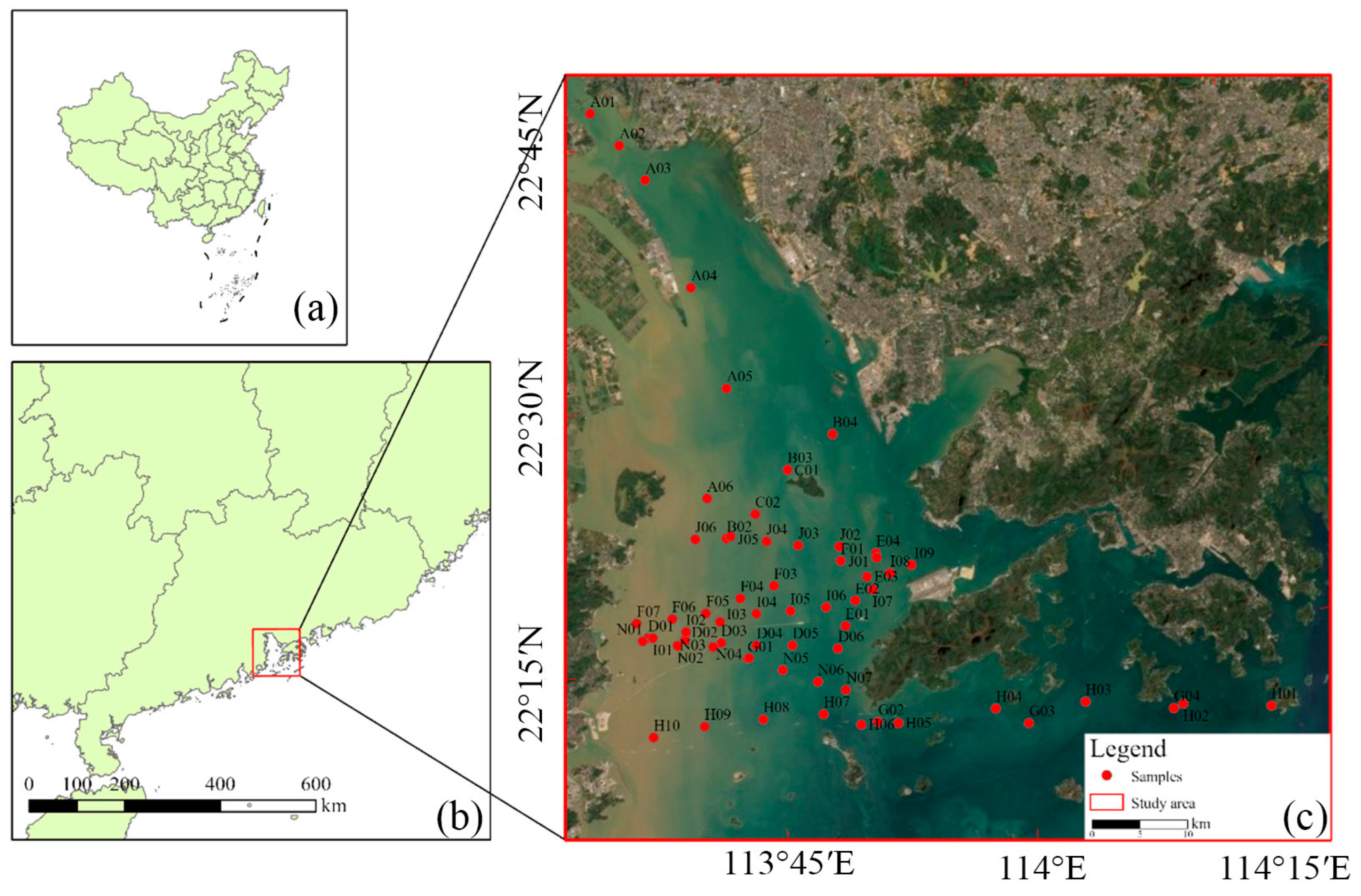
2.1. Study Region

The PRE is situated in southern Guangdong Province, China, ranging from 22°N to 22.75°N and 113.5°E to 114°E. It is a significant component of the Greater Bay Area, which encompasses Guangdong, Hong Kong, and Macau, and is widely regarded as a crucial economic zone in China. Due to its strategic location and abundant natural resources, the development of the PRE has been a key driver of economic growth (Figure 1). With rapid population growth and urbanization, water quality is threatened by various factors such as terrestrial waste, sewage, industrial discharges, and more. Thus, it is particularly important to monitor water quality and respond quickly to different pollution events in the PRE. Due to inland water discharges, the PRE has unique water quality characteristics that differ from those of continental shelf waters [34].

2.2. In-Situ Data Collection

2.2.1. Sample Collection and Processing

A cruise survey was carried out in the PRE in May 2014 to investigate its unique water properties. During the survey, measurements were taken of surface optical radiation, and water samples were collected, filtered, and stored for later analysis. We measured the concentrations of Chl-a, suspended particulate matter (SPM), and CDOM absorption coefficients at a laboratory in less than one week. In the cruise survey, water samples were gathered from a depth of 0–1 m and stored in acid-washed polyvinyl chloride bottles, under dark and refrigerated conditions, to assess CDOM absorption [35]. With pre-combustion Whatman GF/F filters, large particles, and plankton cells were first filtered out of water samples at low pressure, and next, Nitrocellulose Millipore filters with a 0.22 µm pore size were used to filter the samples. The CDOM absorbance (A(λ)) was determined by measuring it in a 10 cm cuvette by using a Shimadzu UV-2550 spectrophotometer at wavelengths of 190–900 nm with 0.25 nm spectral resolution. Finally, the average absorption coefficient of every wavelength was calculated using Equation (1) and corrected for scattering effects by removing the total radioactive absorbance at 700 nm through an infra-red swab pattern (Equation (2)) [36].

$$a_g(\lambda {)}^{\prime }=2.303\times \mathrm{A}(\lambda )/r,$$

(1)

$$a_g\left(\lambda \right)=a_g(\lambda {)}^{\prime }-a_g(700{)}^{\prime }\times \lambda /700$$

(2)

where λ represents wavelength, A(λ) indicates the measured absorbance, a_g(λ) is the absorption coefficient in m⁻¹, a′ is the uncorrected absorption coefficient in m⁻¹, and r represents the cuvette length in m. As previous studies showed that the absorption coefficient at 290 nm, a_g(290) had the strongest correlation with Landsat-8 OLI image reflectance [5], the a_g(290) was used to be an indicator of the CDOM concentration for algorithm development.

2.2.2. Measurements of In-Situ and Remote Sensing Reflectance

In-situ data in the PRE were collected during a cruise survey in the period from 3 to 11 May 2014. A total of 15 transects were covered in the estuary and one was recovered to the south of Hong Kong during the cruise, as shown in Figure 1c, with 59 sampling stations. At each station, water surface reflectance spectra were measured by using an OceanOptics spectrometer with a spectral resolution of 0.2 nm in a range from 380 nm to 1000 nm. During the survey, in-situ spectral measurements were collected for downwelling irradiance above the water surface (E_s(λ,θ,ϕ)), total water-leaving radiance (L_t(λ,θ,ϕ)), and sky radiance (L_sky(λ,θ″,ϕ)) at a nadir viewing angle (θ) of 45° and an azimuthal angle (ϕ) of 135° relative to the sun, where θ ″ represents the solar zenith angle. These measurements were carried out following the protocols outlined by Mobley to eliminate sun glint effects [37]. In addition, the spectrometer prober was placed 2 m above the water surface when conducting the measurements to prevent shadows and boat reflections. The remote sensing reflectance (R_rs) was derived by the equation given by [38],

$$R_{rs}(\theta ,\varphi ,\lambda )=\frac{L_t(\theta ,\varphi ,\lambda )-\rho (\theta ,\varphi )L_{sky}\left({\theta }^{″},\varphi ,\lambda \right)}{E_s\left(\lambda \right)}$$

(3)

where ρ(θ,ϕ) is the reflectance of the air-water interface, obtained from a Look-Up-Table [39], based on the sensor geometry setting, including sun zenith and azimuth angles, and wind speed. The R_rs was calculated from the filtered dataset based on the median spectrum, according to the procedure described by Maciel et al. [40].

Water surface spectra were measured within a zenith angle of 45 degrees and a solar azimuth of 135 degrees. The reflectance was calculated as the ratio between the surface reflectance and the spectral target of the reference panel. Ten measurements were taken at each site, and a representative spectrum was calculated as the geometrical mean of all samples, excluding wild-type values. Then, the data were converted to remote sense reflectance by dividing the reflectance factor by π.

In addition, to reduce the uncertainty in the spectra, the acquired data were manually filtered to exclude outliers or scintillation-contaminated spectra. Finally, the spectral response function (SRF) of the Landsat-8 OLI sensor was simulated using the R_rs spectra [41].

2.3. Methods

2.3.1. Image Preprocessing

Landsat-8 OLI images of the PRE were obtained from the United States Geological Survey (USGS) portal (https://earthexplorer.usgs.gov/ accessed on 31 December 2022). These data feature a temporal resolution of 16 days and a spatial resolution of 30 m, and include four visible bands, one near-infrared band, and two short-wave infrared bands. The Landsat 8 OLI also has a shorter blue band and a narrower near-IR band than Landsat 4/5/7, enabling better monitoring of water quality parameters in coastal waters. Only images with less than 10% cloud coverage were used in this study. The satellite images were corrected for atmospheric effects through the application of the OLI “lite” (ACOLITE) atmospheric correction process. Previous studies showed that ACOLITE has better overall performance on Landsat 8 images [42]. In addition, the Normalized Difference Water Index (NDWI) [14] was calculated for all images to separate water bodies from shadows formed by land or terrain, based on contrast thresholds for near-infrared and visible green radiation.

2.3.2. Machine Learning Approaches

In this study, to establish a dependable remote sensing algorithm, six machine learning techniques were employed for estimating a_g(290) in the PRE waters. These techniques were Support Vector Regression (SVR), Random Forest (RF), Extreme Gradient Boosting Decision Tree (XGBoost), Convolutional Neural Network (CNN), K-nearest Neighbor Regression (KNN), and Multi-Layer Perception (MLP), based on the in-situ survey data collected in the PRE.

• Support Vector Regression

The Support Vector Regression (SVR) is a kernel-based, supervised algorithm that was first introduced by Cortes and Vapnik in 1995 for binary classification [43]. It employs a statistical theoretical approach that differs from traditional statistical methods and is based on an approximation of the structured risk minimization method. SVR is considered a shallow machine learning technique that can address a range of issues, such as small sample sizes, nonlinear relationships, high-dimensional pattern recognition, and overfitting of functions. The algorithm’s versatility and ability to handle complex data have made it a popular choice in various fields.

• Random Forest

The Random Forest (RF) algorithm is a versatile machine learning technique that can be used to tackle both regression and classification problems [44]. It is based on decision trees, which split a variable space consisting of n variables of c₁, c₂, c₃, …, and c_n into j distinct regions of R₁, R₂, R₃, …, and R_j. The final prediction for each input is obtained by combining the predictions made by all decision trees in the Random Forest (RF) algorithm [44]. This is done by taking the average of the predictions, reducing variance, and improving accuracy. The RF algorithm can be adjusted using hyperparameters such as the number of trees, maximum depth, and split criteria, making it flexible and adaptable to various problems and data types. The configuration of the RF algorithm involves several hyperparameters, such as the number and maximum depth of decision trees. In this case, the RF model was implemented using the Random Forest package in the python environment and consisted of 100 decision trees with a maximum of five leaf nodes.

• Extreme Gradient Boosting

Extreme Gradient Boosting (XGBoost) is a recent and popular implementation of the Gradient Boosting algorithm, which is a machine learning technique used for both regression and classification problems [45]. The XGBoost is a powerful ensemble learning algorithm based on the principles of decision tree. Unlike RF, XGBoost employs a boosted merging technique that combines weak learners into a single, strong model through an additive strategy. This feature makes XGBoost a versatile and highly effective solution for a range of machine learning problems. The XGBoost training process starts by fitting one learner with the entire dataset, and then adding a second learner to fit the residual error of the entire dataset. A second learner is added for the remaining error of the entire dataset to fit the remaining error from a previous learner [38]. The training is repeated until the threshold is reached. Final prediction results are summed up from each learner’s predictions. This method is implemented using the python package for XGBoost. The main parameters that determine the structure of the model include the number of gradient boosting trees and the maximum tree depth. The number of gradient boosting trees used in this example was 50, and the maximum tree depth was 5.

• K-Nearest Neighbor

The K-nearest neighbor regression (KNN) is a simple and easy-to-implement method for predicting continuous data with multiple variables. The prediction of each of the experiments is calculated as the weighted average of the response variable k nearest sample in the set of training, where k is an integer of the value of the user’s specified value. In each characteristic space, the distance between the training and test sample squared is estimated using the given measure of distance, known as a distance metric. The weight is then defined as the reciprocal of the square root of the sum of the distances in all feature spaces. The parameters of the K-Nearest Neighbor (KNN) method, including the values of k and the distance metric, play a crucial role in determining the performance and efficiency of the method.

• Multi-Layer Perceptron

Multi-Layer Perceptron (MLP) is a type of artificial neural network that consists of three key layers: an input layer, a hidden layer, and an output layer. In the input layer, each sample in the dataset is transformed into a feature vector, which is then processed by nodes in the hidden layer. The hidden layer nodes receive data from the input layer and apply a non-linear activation function, such as sigmoid or ReLU, to this data. Finally, the output layer generates the final prediction based on the data processed by the hidden layer.

• Convolutional Neural Network

Convolutional Neural Networks (CNNs) are prominent types of feed-forward neural networks, known for their exceptional performance in image recognition and natural language processing (NLP) tasks. The architecture of CNNs comprises three crucial components, each playing a critical role in processing and analyzing data. The first component is the convolutional layer, which consists of multiple feature planes that are responsible for detecting unique features in the input data. The feature layer on each neuron is local to the previous feature layer through the convolutions kernel, which slides across the feature planes with a specific step size to attain weight sharing. The function of the pooling layer is to downsample the local features extracted by the convolutional layer, reduce the network-free parameters, improve robustness, and enhance the robustness of the feature data. Typically, average pooling or maximum pool methods are used. The fully connected layer takes the output of the features from the pooling layer and fully connects it to the multi-layer perceptron. The fully connected layer acts as the final output layer in a Convolutional Neural Network (CNN), producing the predictions based on the features learned from the previous layers. It is essential to have this layer in the network, as it allows for the integration of all the features learned by the network into a single prediction. The multi-layer perceptron in the fully connected layer is trained using a supervised learning method to make predictions based on the input data. The integration of these three components in the CNN architecture renders it an effective instrument for image recognition and natural language processing (NLP), as well as for water quality research applications. The CNN model detailed in this paper comprised 32 convolutional layers, five activation layers, a stretching layer, a fully connected layer, and an output layer. It was developed using the Python programming language and the Keras framework.

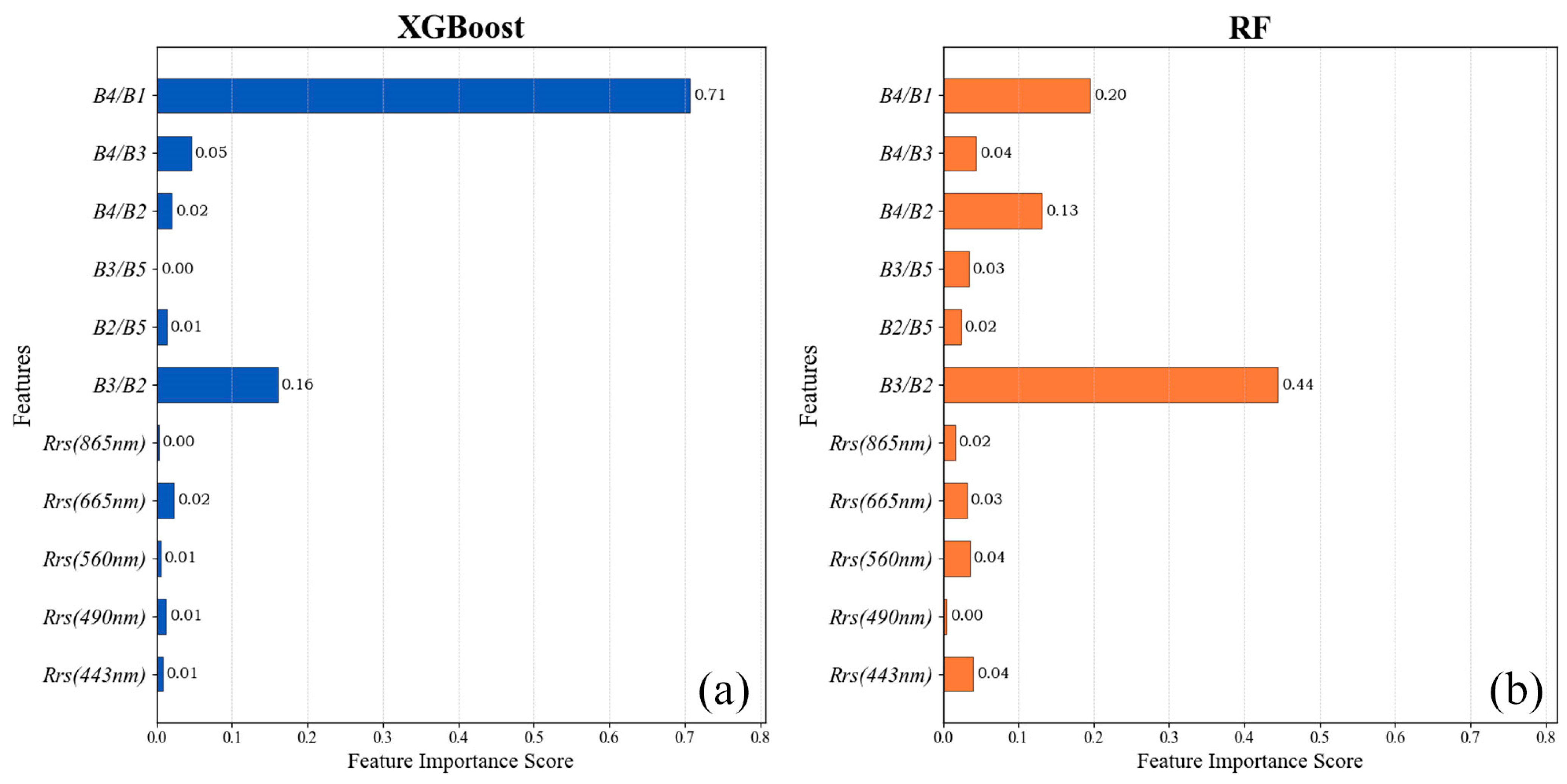
2.3.3. Feature Selection

The use of spectral indices as input features has been shown to improve the model performance in previous studies [46]. In model training, the correlation analysis between each OLI band and band combination is performed. The determination of the CDOM absorption coefficient is carried out using Pearson correlation analysis, with the bands exhibiting the highest correlations being selected as inputs for the machine learning model. Our results showed that 11 spectral variables could be selected as inputs: R_rs for the first five bands of the OLI (443, 482, 561, 655, and 865 nm), the green-blue ratio index (GBI), the blue-near-infrared ratio index (BNIRI), the green-near ratio index (GNI), the red-blue ratio index (RBI), the red-green ratio index (RGI), and the red-near ratio index (RCI). Then, a_g(290) was used as the output element. However, the SVR algorithm uses five single bands as inputs (

Table 1. The input bands and band combinations of the Landsat 8 OLI.

Sensors	Band	Band-Ratio
Landsat-8 OLI	B1 (443 nm)	B2/B5 (BNIRI)
	B2 (482 nm)	B3/B2 (GBI)
	B3 (561 nm)	B3/B5(GNI)
	B4 (655 nm)	B4/B1(RCI)
	B5 (865 nm)	B4/B2(RBI)
		B4/B3(RGI)

), as it will present better results.

After the machine learning algorithm training process, we evaluated the importance of the variables and observed which variables had the highest predictive capability in the developed model.

2.3.4. Accuracy Assessment

In this study, 70% of the data were used for algorithm training and 30% for validation. To assess the credibility of the results, several metrics were computed, including determination (R²), slope (linear regression), root mean square error (RMSE), mean absolute percentage error (MAPE), bias (systematic error), and mean absolute error (MAE). R², RMSE, and MAPE are widely used to evaluate model performance based on the original data distribution. The MAE is calculated in log-transformed space, and deviation represents the residuals in logarithmic form. The deviation and MAE calculated in log-transformed space are considered to provide a good evaluation of the algorithm for the log-normal distribution of water quality [23,46]. These measures are much more robust and straightforward and are the measure of evaluation for remote sensing algorithms with logarithmic distributions [47], written as

$$\mathrm{R}\mathrm{M}\mathrm{S}\mathrm{E}=\frac{1}{N}\sqrt{{\sum }_{i=1}^N {\left(M_i-E_i\right)}^2},$$

(4)

$$\mathrm{M}\mathrm{A}\mathrm{P}\mathrm{E}=\frac{1}{N}\sum ^N \frac{\left|M_i-E_i\right|}{M},$$

(5)

$$\mathrm{BIAS}={10}^{\left(\frac{\sum _{i=1}^N {\mathrm{l}\mathrm{o}\mathrm{g}}_{10}\left(M_i\right)-\mathrm{l}\mathrm{o}\mathrm{g}10\left(E_i\right)}{N}\right)},$$

(6)

$$\mathrm{M}\mathrm{A}\mathrm{E}=\frac{{\sum }_{i=1}^n\left|M_i-E_i\right|}{n}$$

(7)

where N represents the number of data pairs, the subscript i refers to a single data point, and M and E stand for measured and estimated values, respectively.

3. Results

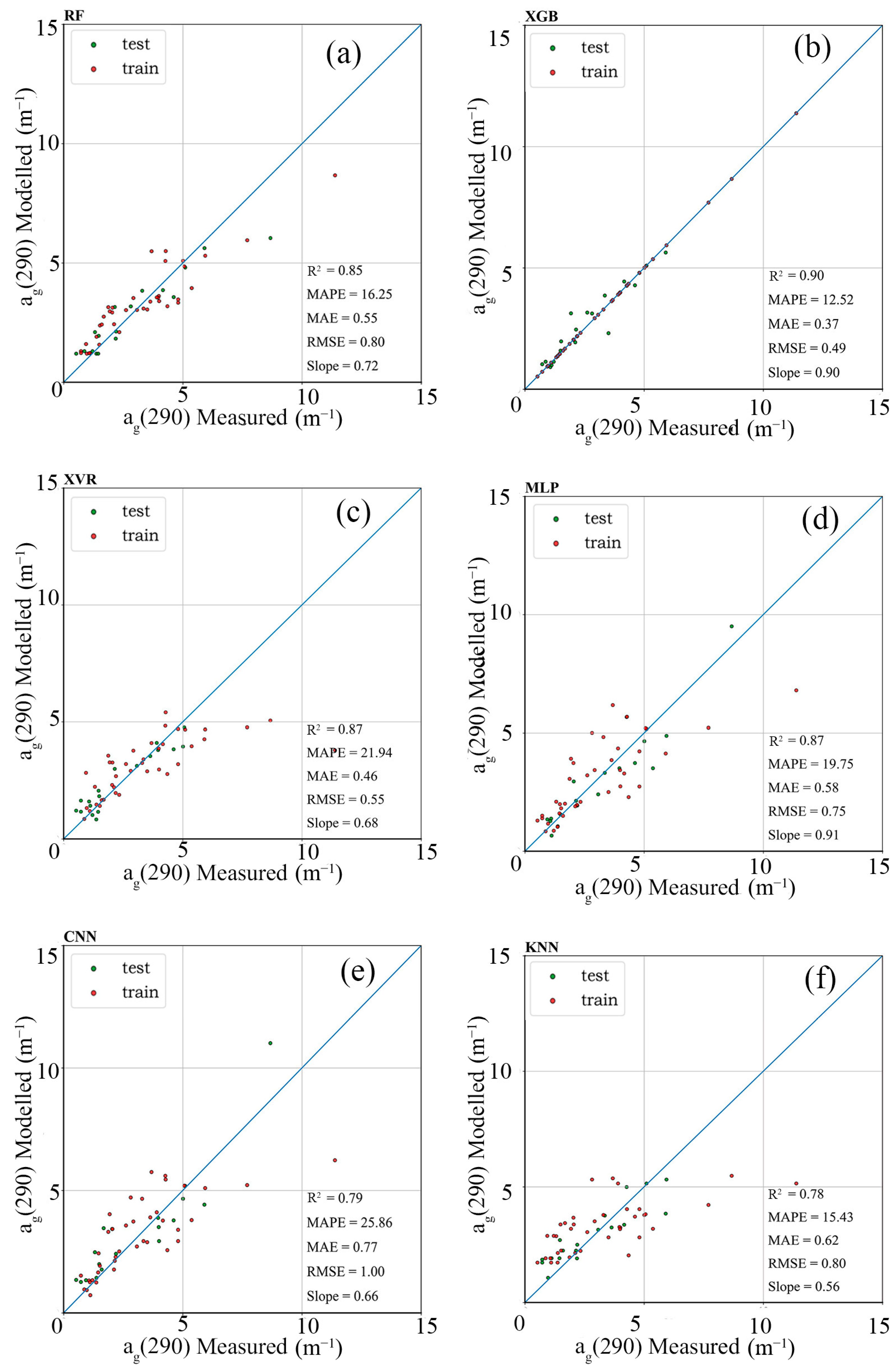
3.1. Algorithm Accuracy Analysis

Table 2. Validation results of the six machine learning algorithms determined from the test dataset.

	Machine Learning Algorithms
Statistic	RF	SVM	XGBoost	KNN	MLP	CNN
R2	0.85	0.87	0.9	0.78	0.87	0.79
BIAS	0.05	−0.09	−0.11	−0.16	0.12	0.03
MAPE (%)	16.25	21.94	12.52	15.43	19.75	25.86
MAE (m−1)	0.55	0.46	0.37	0.62	0.58	0.77
RMSE (m−1)	0.8	0.55	0.49	0.8	0.75	1

and Figure 2 show the accuracies of the six machine learning algorithms for the test dataset. The results indicated the potential of these six machine learning algorithms for CDOM estimation in the PRE. The XGBoost algorithm outperformed the other five machine learning algorithms in almost all statistical metrics. MAPE for the XGBoost was 12.52%, followed by the KNN (15.43%), RF (16.25%), MLP (19.75%), SVM (21.94%), and CNN (25.86%). The R² value was 0.9 for the XGBoost, followed by the SVM and MLP (0.87), RF (0.85), CNN (0.79), and KNN (0.78). The RF had the highest stability in the validation results (with R² = 0.85, BIAS = 0.05, MAPE = 16.25%, MAE = 0.55 m⁻¹, and RMSE = 0.8 m⁻¹). Overall, the six machine learning algorithms achieved over 75% accuracy in estimating the CDOM with the available data.

To further illustrate the performance of the six machine learning methods for CDOM retrieval, scatterplots of in-situ measured CDOM a_g(290) versus estimated CDOM a_g(290) were generated and are displayed in Figure 2. We observed that the XGBoost had a a_g(290) wider range (0 to up to 12.0 m⁻¹), providing more realistic CDOM a_g(290) estimates, while the XVR and KNN had less estimate range, which tended to underestimate the CDOM. The RF also showed underestimated CDOM values, while the MLP and CNN revealed a more discrete pattern, indicating their instability in predicting the CDOM values.

Figure 3 illustrates the importance of the input parameters in the XGBoost and RF algorithms, as these two algorithms had the best performance in estimating CDOM values. For XGBoost, the most important input parameters (measured by Gain) were B4/B1 (red/blue1) and B3/B2 (green/blue2) ratios, accounting for 69% and 18% of the importance percentage, respectively. This indicated that B4/B1 and B3/B2 were more sensitive to CDOM values than other input variables. For the RF algorithm, the most important input parameters were B3/B2 (green/blue) and B2/B1 (blue2/blue1) ratios, accounting for 45% and 18% of the importance percentage, respectively. Both algorithms suggested that the red/green/blue2 over blue1 ratios were the critical input parameters that revealed the fluorescence effects caused by ultraviolet wavelengths for CDOM. CDOM absorbs ultraviolet light that may induce fluorescence in the visible bands [5].

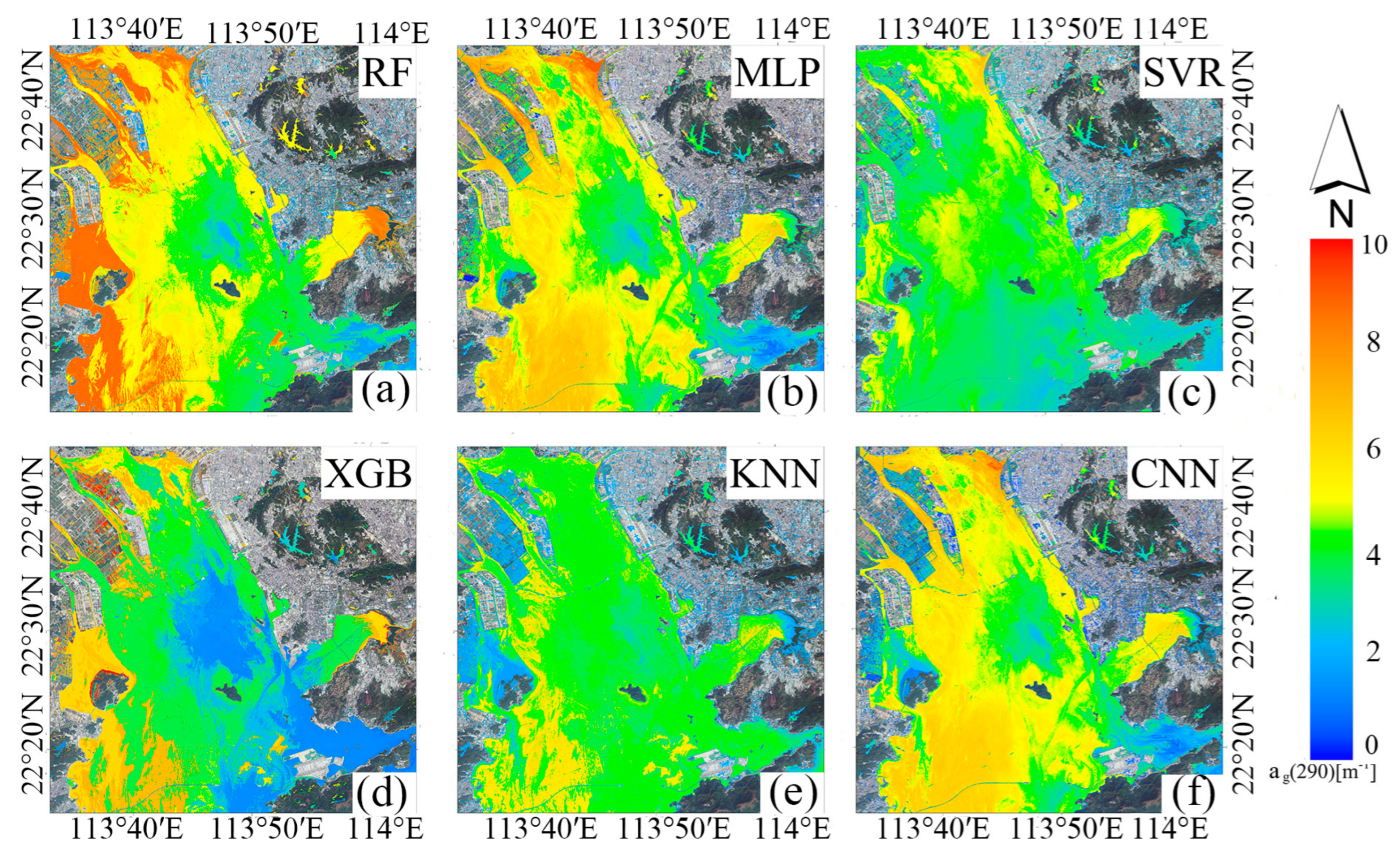
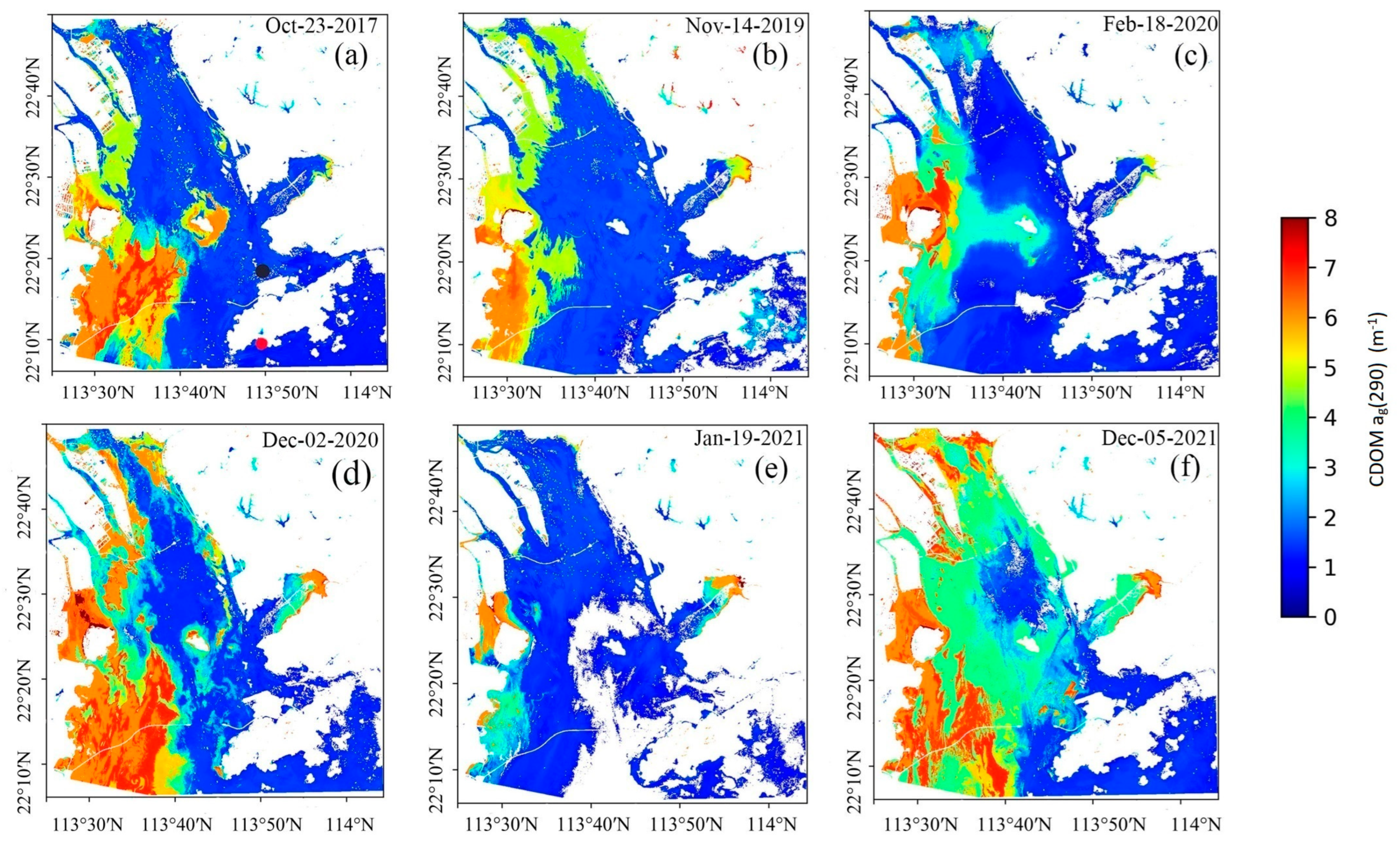
3.2. CDOM Spatial Patterns in the PRE

To further reveal the CDOM estimation capability from different algorithms, six machine learning algorithms developed in this study were applied to Landsat 8 OLI images to estimate the CDOM absorption coefficient in the PRE. The estimated CDOM values are shown in Figure 4. We observed that the western nearshore of the PRE region showed higher concentrations, while the continental shelf and Hong Kong nearshore displayed lower concentrations, and the central part of the PRE exhibited a lower concentration.

Figure 4 reveals that there were differences in estimated CDOM values from these algorithms. The KNN and SVR algorithms generated lower CDOM concentrations on the west side of the estuary than those from the XGBoost estimates; however, the RF provided higher CDOM values in this area (on the west side of the PRE). For the MLP and CNN algorithms, the estimated CDOM values were high on both sides of the estuary, revealing unrealistic results due to the fact that the major outlets of the river discharges are all located on the west side of the PRE and, therefore, the CDOM should be much higher on the west side of the PRE. The CDOM values estimated from the XGBoost algorithm in the PRE had a wide range, consistent with the model validation results (as shown in Figure 2).

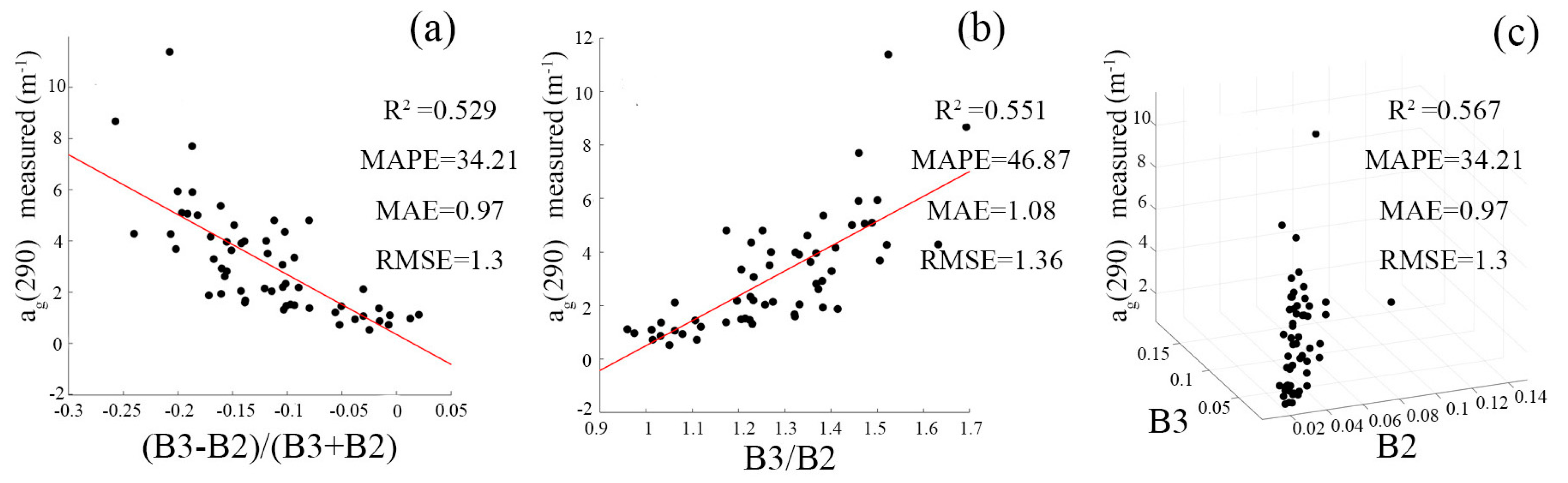
3.3. Comparison with Other Models

Using the same cruse dataset, Lei et al. developed an empirical CDOM algorithm for PRE with the band-ratio of B3/B1, and the R² of the CDOM algorithm reached 0.79 and the MAPE was 32% [5]. Zhao et al., used the Support Vector Machine (SVM) machine learning algorithm to estimate CDOM concentrations in the PRE by inputting two band ratios, achieving a validation accuracy with an R² of 0.84 [48]. Liu et al. developed an algorithm for estimating CDOM and DOC concentrations in the PRE using two band ratios, specifically R_rs(667)/R_rs(443) and R_rs(748)/R_rs(412), with a correlation coefficient of 0.698 [49]. Nevertheless, at present, the exploration of employing machine learning algorithms to infer CDOM concentrations in this region remains relatively limited and, therefore, with a higher R² value, the machine learning model we established unveils fresh and novel results.

To consolidate this conclusion, band-ratios/combination CDOM models were trained (or calibrated) using the in-situ data collected in this study.

Here, three ratios/combination algorithms are given by [25],

$$a_g\left(290\right)=\mathrm{A}\frac{\mathrm{B}3-\mathrm{B}2}{\mathrm{B}3+\mathrm{B}2}+\mathrm{C}$$

(8)

$$a_g\left(290\right)=\mathrm{A}\frac{\mathrm{B}3}{\mathrm{B}2}+\mathrm{C}$$

(9)

$$a_g\left(290\right)=\mathrm{A}\times \mathrm{B}2+\mathrm{C}\times \mathrm{B}3+\mathrm{D}$$

(10)

where B2 and B3 represent the R_rs values at Landsat-8 bands 2 and 3, respectively, and A, B, and C represent the model calibration coefficients.

The calibration and validation results are shown in

Table 3. Calibration coefficients and R² of empirical CDOM models.

	A	C	D	R2	MAPE	MAE	RMSE
$\mathrm{A}\frac{\mathrm{B}3 - \mathrm{B}2}{\mathrm{B}3 + \mathrm{B}2}+\mathrm{C}$	23.416	0.342	-	0.53	34.21	0.97	1.3
$\mathrm{A}\frac{\mathrm{B}3}{\mathrm{B}2}+\mathrm{C}$	9.302	−8.801	-	0.55	46.87	1.08	1.36
$\mathrm{A}\times \mathrm{B}2+\mathrm{C}\times \mathrm{B}3+\mathrm{D}$	−253.25	230.64	1.43	0.57	23.27	0.93	1.26

and Figure 5, which reveal that the R² of three empirical algorithms were 0.53, 0.55, and 0.57, and the MAPE was 34.21%, 46.87%, and 23.27%, respectively. For the results of R² and MAPE, the machine learning algorithms developed in this study had much better performance than these empirical models and could better simulate the CDOM absorption coefficients in terms of optical spectra. The empirical model exhibited an overall underestimation of the CDOM over 7.0 m⁻¹. Although empirical models are much easier to implement, allowing straightforward extrapolation of predictions beyond the training data set, the machine learning algorithms can retrieve more accurate CDOM absorptions in the PRE from satellite optical reflectance observations.

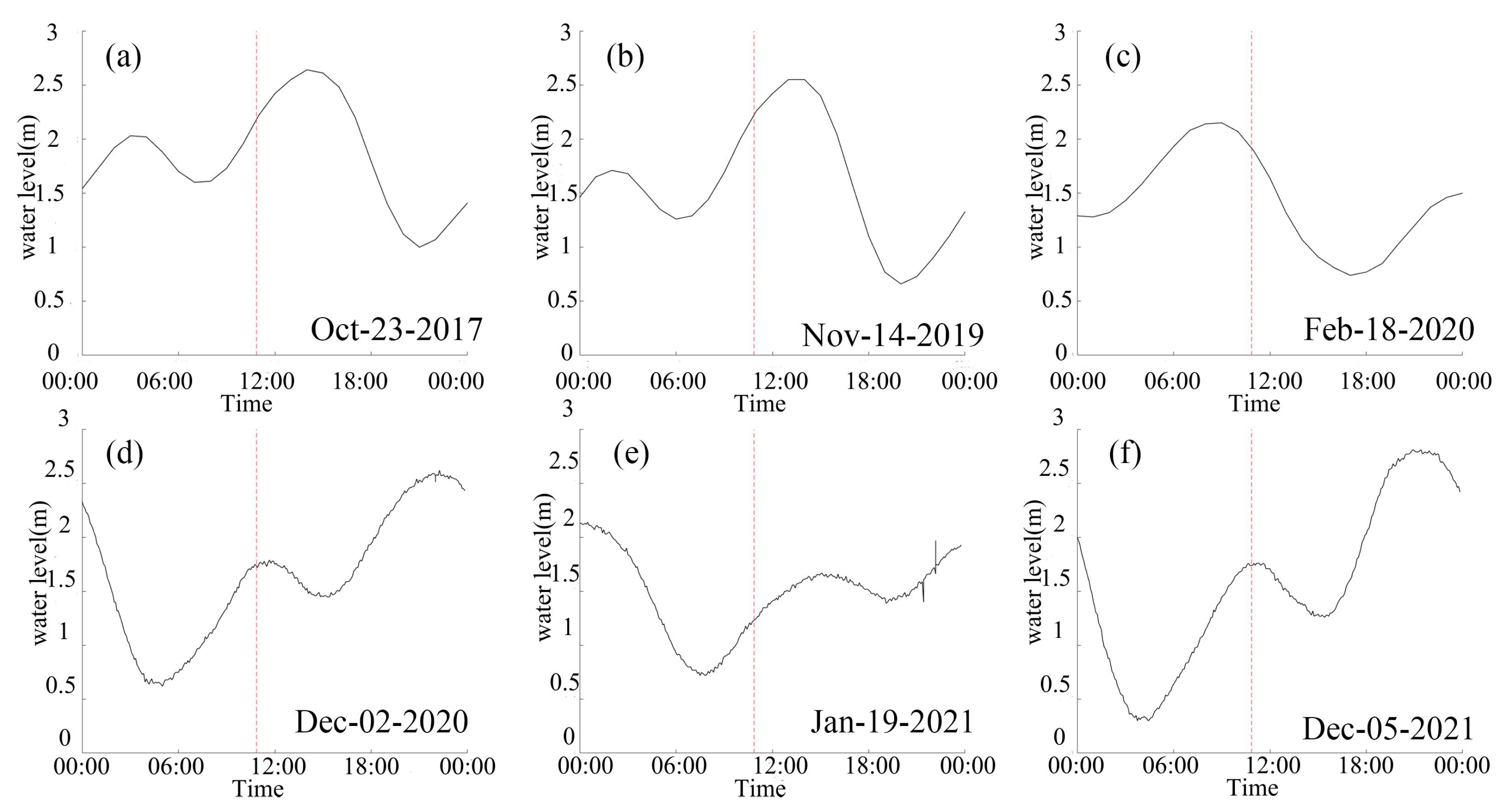
3.4. CDOM Variations in the PRE

In this study, the XGBoost algorithm was further used to derive the CDOM values from the Landsat OLI images, which were acquired on 23 October 2017, 14 November 2019, 18 February 2020, 2 December 2020, 19 January 2021, and 5 December 2021. The local acquisition time of these satellite images was ~10:52 AM for the Landsat-8 sun-synchronous orbit. The derived CDOM data in the PRE are shown in Figure 6, which displays significant difference in the CDOM values for the satellite images at different times.

The CDOM variation in the PRE may be caused by many factors, including hydrodynamic conditions. Figure 7 shows the sea level measurements at the Shek Pik tidal gauge station (22°13′13″N, 113°53′40″) provided by the Hong Kong Observatory, and the satellite image acquisition times are also marked in the figure, which reveals the tidal phases at the satellite image acquisition times. The high CDOM appeared on 2 December 2020 and 5 December 2021 in high water during the tide slack periods (Figure 6). On 23 October 2017 and 14 November 2019, the CDOM values were lower than those on 2 December 2020 and 5 December 2021 (Figure 6). The tidal phases at these two time periods were on the flood with the increasing water level (Figure 7) and, therefore, the onshore-ward surface currents appeared in the estuary. The lowest CDOM of all the cases appeared on 19 January 2021 in the weak flood tide and the water level was elevated from low low-water to low high-water. On 18 February 2020, the water level was decreasing on the ebb tide and the CDOM was higher than that on the weak flood tide and lower than the low high-water.

Table 4. Tidal phase and wind conditions at the satellite image acquisition times.

Date	23 October 2017	14 November 2019	18 February 2020	2 December 2020	19 January 2021	5 December 2021
Tide Phase	Flood	Flood	Ebb	LHW *	Weak flood	LHW *
Tide	Spring	Spring	Neap	Spring	Neap	Spring
Wind speed (m s−1)	4.3	3.3	7.1	5.6	3.9	4.7
Wind Dir	NNE	E	NNE	NNE	SE	N

* LHW-low high-water.

lists the tidal and wind conditions at the satellite acquisition times. The wind data were measured at the Sha Chau meteorological station, available from the web https://data.weather.gov.hk (accessed on 13 December 2022). The southeasterly wind prevailed on 19 January 2021, while the CDOM was the lowest of all the cases and, in addition, it corresponded to a neap tide period. The easterly wind also appeared on 14 November 2019 for one of the two LHW cases, and it seems that the CDOM of this case was lower than that of the other LHW case with northerly winds.

The above analysis suggests that the tidal condition can greatly affect the CDOM distributions in the PRE. The high CDOM appears in the high-water during the tidal slack period, and the CDOM in the weak flood tide was lower than in the strong flood tide. The wind also had impacts on the CDOM distribution, with the low CDOM appearing in the easterly.

The tidal currents can modify the water properties in the estuary, and the results indicate that the shoreward current on the ebb causes the CDOM to be concentrated inside the estuary. In the high-water, the CDOM reached the maximum, forced by the accumulation effects of the onshore-ward tidal current. However, the CDOM spatial pattern may be controlled by many factors, such as river discharge and wind-induced upwelling, in addition to the wind and tidal currents. Lai et al. indicated that the interaction of the wind and tide might modify the Pearl River estuarine circulations, which could change the spatial distributions of nutrients in the estuary [50]. Therefore, a detailed analysis of the CDOM pattern needs to be implemented with more available data in the future.

4. Discussion

This study compared the performance of six machine learning algorithms in estimat-ing CDOM concentrations in the PRE. The results revealed that the XGBoost and SVR algorithms exhibited the highest accuracies, with RMSE of 0.49 m⁻¹ and 0.55 m⁻¹, respectively. In contrast, the MLP, KNN, and RF algorithms displayed moderate accuracies, with RMSEs of 0.75 m⁻¹ and 0.8 m⁻¹, respectively. The CNN algorithm, however, demonstrated the lowest accuracy, with an RMSE of 1.0 m⁻¹. The discrepancies in performance among these algorithms can be attributed to various factors, such as variations in prediction stability and intrinsic limitations and the shortcomings of each algorithm. For instance, neural network-based algorithms tend to be highly sensitive to hyperparameter selection and may require a larger amount of training data to achieve optimal performance.

The increasing importance of machine learning in the remote sensing monitoring of water quality, particularly with large amounts of data analysis, has been realized recently. However, machine learning is a black-box method, and data overfitting could occur in some cases. Therefore, understanding the model decision process in the black box is crucial. Recently proposed explainable methods, such as Local Interpretable Model-agnostic Explanations (LIME) [51] and Shapley Additive explanations (SHAP) [52], can make the machine learning black box transparent and help interpret water quality retrieval processes. Thus, combining machine learning and explainable methods will contribute to developing robust results for machine learning algorithms.

This study highlights that the high accuracy of machine learning methodologies enables the implementation of real-time CDOM monitoring using satellite observation data in the PRE, which is significant for improving water quality in estuarine waters with varying optical complexity. Although machine learning algorithms mostly outperform traditional methodologies, accurate estimation of CDOM from satellite remote sensing remains challenging due to CDOM’s specific absorption and reflectance characteristics. Consequently, effectively combining various types of satellite observations is essential for developing a more robust model.

With more satellite and in-situ observations available in the future, the training and testing datasets can be further consolidated, potentially leading to more reliable results in machine learning algorithm development. Since machine learning is a black-box method that cannot provide distinct physical meanings for remote sensing algorithms, our future work may focus on developing explainable methods for these machine learning models to help interpret feature importance and identify the factors that influence the model’s decision-making process.

5. Conclusions

In this study, we developed machine learning algorithms based on a cruise dataset to retrieve CDOM absorption coefficients from Landsat OLI image data in the PRE. With reliable algorithms resulting from this study, CDOM data in the PRE can be retrieved from long-term archived Landsat images, which will help in capturing CDOM variabilities on different time scales in the PRE and understanding ecological environment changes in the area. Six machine learning algorithms for CDOM were developed using cruise-measured CDOM absorption coefficients and optical spectral R_rs. The results show that XGBoost presented the best performance in estimating CDOM, validated by a test dataset. The estimated CDOM from XGBoost had the highest range and the lowest error, and when applied to Landsat-8 image data, the XGBoost algorithm provided reasonable CDOM estimations in the PRE compared to the other machine learning algorithms. We used XGBoost algorithms to retrieve CDOM values from Landsat data acquired on 23 October 2017, 14 November 2019, 18 February 2020, 2 December 2020, 19 January 2021, and 5 December 2021. The results suggest that tide and wind can significantly affect CDOM spatial patterns in the PRE. High CDOM appears during high water in the tidal slack period, and CDOM in the weak flood tide is lower than in the strong flood tide. Easterly wind can weaken CDOM in the estuary.

References

1. Zhang, Y.; Zhou, L.; Zhou, Y.; Zhang, L.; Yao, X.; Shi, K.; Jeppesen, E.; Yu, Q.; Zhu, W. Chromophoric Dissolved Organic Matter in Inland Waters: Present Knowledge and Future Challenges. Sci. Total Environ. 2021, 759, 143550. [Google Scholar] [CrossRef]
2. Siegel, D.A.; Maritorena, S.; Nelson, N.B.; Hansell, D.A.; Lorenzi-Kayser, M. Global Distribution and Dynamics of Colored Dissolved and Detrital Organic Materials. J. Geophys. Res. 2002, 107, 21-1–21-14. [Google Scholar] [CrossRef]
3. Carder, K.L.; Steward, R.G.; Harvey, G.R.; Ortner, P.B. Marine Humic and Fulvic Acids: Their Effects on Remote Sensing of Ocean Chlorophyll. Limnol. Oceanogr. 1989, 34, 68–81. [Google Scholar] [CrossRef]
4. Gholizadeh, M.H.; Melesse, A.M.; Reddi, L. A Comprehensive Review on Water Quality Parameters Estimation Using Remote Sensing Techniques. Sensors 2016, 16, 1298. [Google Scholar] [CrossRef] [Green Version]
5. Lei, X.; Pan, J.; Devlin, A. An Ultraviolet to Visible Scheme to Estimate Chromophoric Dissolved Organic Matter Absorption in a Case-2 Water from Remote Sensing Reflectance. Front. Earth Sci. 2020, 14, 384–400. [Google Scholar] [CrossRef]
6. Rochelle-Newall, E.J.; Fisher, T.R. Chromophoric Dissolved Organic Matter and Dissolved Organic Carbon in Chesapeake Bay. Mar. Chem. 2002, 77, 23–41. [Google Scholar] [CrossRef]
7. Zhou, Y.; Yao, X.; Zhang, Y.; Shi, K.; Zhang, Y.; Jeppesen, E.; Gao, G.; Zhu, G.; Qin, B. Potential Rainfall-Intensity and pH-Driven Shifts in the Apparent Fluorescent Composition of Dissolved Organic Matter in Rainwater. Environ. Pollut. 2017, 224, 638–648. [Google Scholar] [CrossRef]
8. Zhang, Y.; Liu, X.; Wang, M.; Qin, B. Compositional Differences of Chromophoric Dissolved Organic Matter Derived from Phytoplankton and Macrophytes. Org. Geochem. 2013, 55, 26–37. [Google Scholar] [CrossRef]
9. Al-Kharusi, E.S.; Tenenbaum, D.E.; Abdi, A.M.; Kutser, T.; Karlsson, J.; Bergström, A.-K.; Berggren, M. Large-Scale Retrieval of Coloured Dissolved Organic Matter in Northern Lakes Using Sentinel-2 Data. Remote Sens. 2020, 12, 157. [Google Scholar] [CrossRef] [Green Version]
10. Feng, Q.; An, C.; Chen, Z.; Owens, E.; Niu, H.; Wang, Z. Assessing the Coastal Sensitivity to Oil Spills from the Perspective of Ecosystem Services: A Case Study for Canada’s Pacific Coast. J. Environ. Manag. 2021, 296, 113240. [Google Scholar] [CrossRef]
11. Tang, D.; Kawamura, H.; Lee, M.-A.; Van Dien, T. Seasonal and Spatial Distribution of Chlorophyll-a Concentrations and Water Conditions in the Gulf of Tonkin, South China Sea. Remote Sens. Environ. 2003, 85, 475–483. [Google Scholar] [CrossRef]
12. Duan, H.; Ma, R.; Hu, C. Evaluation of Remote Sensing Algorithms for Cyanobacterial Pigment Retrievals during Spring Bloom Formation in Several Lakes of East China. Remote Sens. Environ. 2012, 126, 126–135. [Google Scholar] [CrossRef]
13. Lee, Z.; Lubac, B.; Werdell, J.; Arnone, R. An Update of the Quasi-Analytical Algorithm (QAA_v5); International Ocean Colour Coordinating Group Dartmouth: Dartmouth, NS, Canada, 2009; pp. 1–9. [Google Scholar]
14. Lee, Z.; Carder, K.L.; Arnone, R.A. Deriving Inherent Optical Properties from Water Color: A Multiband Quasi-Analytical Algorithm for Optically Deep Waters. Appl. Opt. 2002, 41, 5755–5772. [Google Scholar] [CrossRef]
15. Aurin, D.A.; Dierssen, H.M. Advantages and Limitations of Ocean Color Remote Sensing in CDOM-Dominated, Mineral-Rich Coastal and Estuarine Waters. Remote Sens. Environ. 2012, 125, 181–197. [Google Scholar] [CrossRef]
16. Cao, F.; Tzortziou, M.; Hu, C.; Mannino, A.; Fichot, C.G.; Del Vecchio, R.; Najjar, R.G.; Novak, M. Remote Sensing Retrievals of Colored Dissolved Organic Matter and Dissolved Organic Carbon Dynamics in North American Estuaries and Their Margins. Remote Sens. Environ. 2018, 205, 151–165. [Google Scholar] [CrossRef]
17. Griffin, C.G.; Frey, K.E.; Rogan, J.; Holmes, R.M. Spatial and Interannual Variability of Dissolved Organic Matter in the Kolyma River, East Siberia, Observed Using Satellite Imagery. J. Geophys. Res. 2011, 116, G03018. [Google Scholar] [CrossRef] [Green Version]
18. Joshi, I.D.; D’Sa, E.J.; Osburn, C.L.; Bianchi, T.S.; Ko, D.S.; Oviedo-Vargas, D.; Arellano, A.R.; Ward, N.D. Assessing Chromophoric Dissolved Organic Matter (CDOM) Distribution, Stocks, and Fluxes in Apalachicola Bay Using Combined Field, VIIRS Ocean Color, and Model Observations. Remote Sens. Environ. 2017, 191, 359–372. [Google Scholar] [CrossRef]
19. Mannino, A.; Novak, M.G.; Hooker, S.B.; Hyde, K.; Aurin, D. Algorithm Development and Validation of CDOM Properties for Estuarine and Continental Shelf Waters along the Northeastern U.S. Coast. Remote Sens. Environ. 2014, 152, 576–602. [Google Scholar] [CrossRef]
20. Palmer, S.C.J.; Hunter, P.D.; Lankester, T.; Hubbard, S.; Spyrakos, E.; Tyler, A.N.; Présing, M.; Horváth, H.; Lamb, A.; Balzter, H.; et al. Validation of Envisat MERIS Algorithms for Chlorophyll Retrieval in a Large, Turbid and Optically-Complex Shallow Lake. Remote Sens. Environ. 2015, 157, 158–169. [Google Scholar] [CrossRef] [Green Version]
21. Cao, Z.; Ma, R.; Duan, H.; Xue, K. Effects of Broad Bandwidth on the Remote Sensing of Inland Waters: Implications for High Spatial Resolution Satellite Data Applications. ISPRS J. Photogramm. Remote Sens. 2019, 153, 110–122. [Google Scholar] [CrossRef]
22. Ye, H.; Tang, S.; Yang, C. Deep Learning for Chlorophyll-a Concentration Retrieval: A Case Study for the Pearl River Estuary. Remote Sens. 2021, 13, 3717. [Google Scholar] [CrossRef]
23. Pahlevan, N.; Smith, B.; Schalles, J.; Binding, C.; Cao, Z.; Ma, R.; Alikas, K.; Kangro, K.; Gurlin, D.; Hà, N.; et al. Seamless Retrievals of Chlorophyll-a from Sentinel-2 (MSI) and Sentinel-3 (OLCI) in Inland and Coastal Waters: A Machine-Learning Approach. Remote Sens. Environ. 2020, 240, 111604. [Google Scholar] [CrossRef]
24. Cao, Z.; Ma, R.; Duan, H.; Pahlevan, N.; Melack, J.; Shen, M.; Xue, K. A Machine Learning Approach to Estimate Chlorophyll-a from Landsat-8 Measurements in Inland Lakes. Remote Sens. Environ. 2020, 248, 111974. [Google Scholar] [CrossRef]
25. Sun, X.; Zhang, Y.; Zhang, Y.; Shi, K.; Zhou, Y.; Li, N. Machine Learning Algorithms for Chromophoric Dissolved Organic Matter (CDOM) Estimation Based on Landsat 8 Images. Remote Sens. 2021, 13, 3560. [Google Scholar] [CrossRef]
26. Li, S.; Song, K.; Wang, S.; Liu, G.; Wen, Z.; Shang, Y.; Lyu, L.; Chen, F.; Xu, S.; Tao, H.; et al. Quantification of Chlorophyll-a in Typical Lakes across China Using Sentinel-2 MSI Imagery with Machine Learning Algorithm. Sci. Total Environ. 2021, 778, 146271. [Google Scholar] [CrossRef]
27. Pahlevan, N.; Smith, B.; Alikas, K.; Anstee, J.; Barbosa, C.; Binding, C.; Bresciani, M.; Cremella, B.; Giardino, C.; Gurlin, D.; et al. Simultaneous Retrieval of Selected Optical Water Quality Indicators from Landsat-8, Sentinel-2, and Sentinel-3. Remote Sens. Environ. 2022, 270, 112860. [Google Scholar] [CrossRef]
28. Zhang, Y.; Wu, L.; Ren, H.; Deng, L.; Zhang, P. Retrieval of Water Quality Parameters from Hyperspectral Images Using Hybrid Bayesian Probabilistic Neural Network. Remote Sens. 2020, 12, 1567. [Google Scholar] [CrossRef]
29. Cao, Z.; Ma, R.; Melack, J.M.; Duan, H.; Liu, M.; Kutser, T.; Xue, K.; Shen, M.; Qi, T.; Yuan, H. Landsat Observations of Chlorophyll-a Variations in Lake Taihu from 1984 to 2019. Int. J. Appl. Earth Obs. Geoinf. 2022, 106, 102642. [Google Scholar] [CrossRef]
30. Liu, H.; Li, Q.; Bai, Y.; Yang, C.; Wang, J.; Zhou, Q.; Hu, S.; Shi, T.; Liao, X.; Wu, G. Improving Satellite Retrieval of Oceanic Particulate Organic Carbon Concentrations Using Machine Learning Methods. Remote Sens. Environ. 2021, 256, 112316. [Google Scholar] [CrossRef]
31. Silveira Kupssinskü, L.; Thomassim Guimarães, T.; Menezes de Souza, E.; Zanotta, D.C.; Roberto Veronez, M.; Gonzaga, L.; Mauad, F.F. A Method for Chlorophyll-a and Suspended Solids Prediction through Remote Sensing and Machine Learning. Sensors 2020, 20, 2125. [Google Scholar] [CrossRef] [Green Version]
32. Kim, J.; Jang, W.; Hwi Kim, J.; Lee, J.; Hwa Cho, K.; Lee, Y.-G.; Chon, K.; Park, S.; Pyo, J.; Park, Y.; et al. Application of Airborne Hyperspectral Imagery to Retrieve Spatiotemporal CDOM Distribution Using Machine Learning in a Reservoir. Int. J. Appl. Earth Obs. Geoinf. 2022, 114, 103053. [Google Scholar] [CrossRef]
33. Zhang, Y.; Shi, K.; Sun, X.; Zhang, Y.; Li, N.; Wang, W.; Zhou, Y.; Zhi, W.; Liu, M.; Li, Y.; et al. Improving Remote Sensing Estimation of Secchi Disk Depth for Global Lakes and Reservoirs Using Machine Learning Methods. GIScience Remote Sens. 2022, 59, 1367–1383. [Google Scholar] [CrossRef]
34. Chen, C.; Shi, P.; Yin, K.; Pan, Z.; Zhan, H.; Hu, C. Absorption Coefficient of Yellow Substance in the Pearl River Estuary. In Ocean Remote Sensing and Applications; SPIE: Bellingham, WA, USA, 2003; Volume 4892, pp. 215–221. [Google Scholar]
35. Zhou, Y.; Zhang, Y.; Shi, K.; Niu, C.; Liu, X.; Duan, H. Lake Taihu, a Large, Shallow and Eutrophic Aquatic Ecosystem in China Serves as a Sink for Chromophoric Dissolved Organic Matter. J. Great Lakes Res. 2015, 41, 597–606. [Google Scholar] [CrossRef]
36. Zhang, Y.; Zhang, B.; Ma, R.; Feng, S.; Le, C. Optically Active Substances and Their Contributions to the Underwater Light Climate in Lake Taihu, a Large Shallow Lake in China. Fundam. Appl. Limnol. 2007, 170, 11–19. [Google Scholar] [CrossRef]
37. Mobley, C.D. Estimation of the Remote-Sensing Reflectance from above-Surface Measurements. Appl. Opt. 1999, 38, 7442–7455. [Google Scholar] [CrossRef]
38. Mueller, J.L.; Morel, A.; Frouin, R.; Davis, C.; Arnone, R.; Carder, K.; Lee, Z.P.; Steward, R.G.; Hooker, S.; Mobley, C.D.; et al. Ocean Optics Protocols for Satellite Ocean Color Sensor Validation, Revision 4. Volume III: Radiometric Measurements and Data Analysis Protocols. 2003. Available online: repository.oceanbestpractices.org (accessed on 21 December 2022).
39. Mobley, C.D. Polarized Reflectance and Transmittance Properties of Windblown Sea Surfaces. Appl. Opt. 2015, 54, 4828–4849. [Google Scholar] [CrossRef]
40. Maciel, D.A.; De Moraes Novo, E.M.L.; Barbosa, C.C.F.; Martins, V.S.; Flores Júnior, R.; Oliveira, A.H.; Sander De Carvalho, L.A.; Lobo, F.D.L. Evaluating the Potential of CubeSats for Remote Sensing Reflectance Retrieval over Inland Waters. Int. J. Remote Sens. 2020, 41, 2807–2817. [Google Scholar] [CrossRef]
41. Roy, D.P.; Wulder, M.A.; Loveland, T.R.; Woodcock, C.E.; Allen, R.G.; Anderson, M.C.; Helder, D.; Irons, J.R.; Johnson, D.M.; Kennedy, R.; et al. Landsat-8: Science and Product Vision for Terrestrial Global Change Research. Remote Sens. Environ. 2014, 145, 154–172. [Google Scholar] [CrossRef] [Green Version]
42. Vanhellemont, Q.; Ruddick, K. Turbid Wakes Associated with Offshore Wind Turbines Observed with Landsat 8. Remote Sens. Environ. 2014, 145, 105–115. [Google Scholar] [CrossRef] [Green Version]
43. Cortes, C.; Vapnik, V. Support-Vector Networks. Mach. Learn. 1995, 20, 273–297. [Google Scholar] [CrossRef]
44. Breiman, L. Random Forests. Mach. Learn. 2001, 45, 5–32. [Google Scholar] [CrossRef] [Green Version]
45. Chen, T.; Guestrin, C. XGBoost: A Scalable Tree Boosting System. In Proceedings of the 22nd ACM SIGKDD International Conference on Knowledge Discovery and Data Mining, San Francisco, CA, USA, 13–17 August 2016; Association for Computing Machinery: New York, NY, USA, 2016; pp. 785–794. [Google Scholar]
46. Smith, M.E.; Robertson Lain, L.; Bernard, S. An Optimized Chlorophyll a Switching Algorithm for MERIS and OLCI in Phytoplankton-Dominated Waters. Remote Sens. Environ. 2018, 215, 217–227. [Google Scholar] [CrossRef]
47. Seegers, B.N.; Stumpf, R.P.; Schaeffer, B.A.; Loftin, K.A.; Werdell, P.J. Performance Metrics for the Assessment of Satellite Data Products: An Ocean Color Case Study. Opt. Express 2018, 26, 7404–7422. [Google Scholar] [CrossRef] [Green Version]
48. Zhao, J.; Cao, W.; Xu, Z.; Ai, B.; Yang, Y.; Jin, G.; Wang, G.; Zhou, W.; Chen, Y.; Chen, H.; et al. Estimating CDOM Concentration in Highly Turbid Estuarine Coastal Waters. J. Geophys. Res. Oceans 2018, 123, 5856–5873. [Google Scholar] [CrossRef]
49. Liu, D.; Bai, Y.; He, X.; Pan, D.; Wang, D.; Wei, J.; Zhang, L. The Dynamic Observation of Dissolved Organic Matter in the Zhujiang (Pearl River) Estuary in China from Space. Acta Oceanol. Sin. 2018, 37, 105–117. [Google Scholar] [CrossRef]
50. Lai, W.; Pan, J.; Devlin, A.T. Impact of Tides and Winds on Estuarine Circulation in the Pearl River Estuary. Cont. Shelf Res. 2018, 168, 68–82. [Google Scholar] [CrossRef]
51. Ribeiro, M.T.; Singh, S.; Guestrin, C. Why Should I Trust You? In Proceedings of the 22nd ACM SIGKDD International Conference on Knowledge Discovery and Data Mining—KDD ’16, San Francisco, CA, USA, 13–17 August 2016. [Google Scholar]
52. Lundberg, S.M.; Erion, G.; Chen, H.; DeGrave, A.; Prutkin, J.M.; Nair, B.; Katz, R.; Himmelfarb, J.; Bansal, N.; Lee, S.-I. From Local Explanations to Global Understanding with Explainable AI for Trees. Nat. Mach. Intell. 2020, 2, 56–67. [Google Scholar] [CrossRef]
Figure 1. The Pearl River estuary location in the context of China (a) and part of South China (b). The in-situ survey stations are marked in red dots in the PRE (c).
Remotesensing 15 01963 g001
Figure 2. Scatter plots of in-situ ag(290) versus estimated values from the machine learning algorithms of the RF (a), XGB (b), XVR (c), MLP (d), CNN (e), and KNN (f); the red dots are the training data set and the green dots are the test data set.
Remotesensing 15 01963 g002
Figure 3. Importance percentages of the input parameters for XGBoost (a) and Random Forest (b).
Remotesensing 15 01963 g003
Figure 4. Estimated CDOM ag(290) based on the RF (a), MLP (b), SVR (c), XGB (d), KNN (e), and CNN (f) algorithms from the Landsat-8 OLI image data on 12 May 2021 in the PRE.
Remotesensing 15 01963 g004
Figure 5. Validation results obtained using the empirical algorithm of Equation (8) (a), Equation (9) (b), and Equation (10) (c).
Remotesensing 15 01963 g005
Figure 6. CDOM ag(290) derived from Landsat-8 the OLI data based on the XGBoost algorithm on 23 October 2017 (a), 14 November 2019 (b), 18 February 2020 (c), 2 December 2020 (d), 19 January 2021 (e), and 5 December 2021 (f) in the PRE. The red dot in (a) displays the location of the Shek Pik tidal gauge station, and black dot in (a) shows the location of the Sha Chau meteorological station.
Remotesensing 15 01963 g006
Figure 7. Sea level measured at the Shek Pik tidal gauge station. The tidal data for 23 October 2017 (a), 14 November 2019 (b), 18 February 2020 (c), 2 December 2020 (d), 19 January 2021 (e), and 5 December 2021 (f) in the PRE.
Remotesensing 15 01963 g007