
The Respondence of Wave on Sea Surface Temperature in the Context of Global Change

1
College of Marine Sciences, Shanghai Ocean University, Shanghai 201306, China
2
National Satellite Ocean Application Service, Ministry of Natural Resources, Beijing 100081, China
*
Author to whom correspondence should be addressed.
Remote Sens. 2023, 15(7), 1948; https://doi.org/10.3390/rs15071948
Submission received: 14 February 2023
/
Revised: 21 March 2023
/
Accepted: 4 April 2023
/
Published: 6 April 2023
(This article belongs to the Special Issue Advances in the Ocean Surface Dynamics: Ocean Waves, Wind, and Air-Sea Interaction - in Memory of Professor Shengchang Wen)
Abstract
:Several aspects of global climate change, e.g., the rise of sea level and water temperature anomalies, suggest the advantages of studying wave distributions. In this study, WAVEWATCH-III (WW3) (version 6.07), which is a well-known numerical wave model, was employed for simulating waves over global seas from 1993–2020. The European Centre for Medium-Range Weather Forecasts (ECMWF), Copernicus Marine Environment Monitoring Service (CMEMS), current and sea level were used as the forcing fields in the WW3 model. The validation of modelling simulations against the measurements from the National Data Buoy Center (NDBC) buoys and Haiyang-2B (HY-2B) altimeter yielded a root mean square error (RMSE) of 0.49 m and 0.63 m, with a correlation (COR) of 0.89 and 0.90, respectively. The terms calculated by WW3-simulated waves, i.e., breaking waves, nonbreaking waves, radiation stress, and Stokes drift, were included in the water temperature simulation by a numerical circulation model named the Stony Brook Parallel Ocean Model (sbPOM). The water temperature was simulated in 2005–2015 using the high-quality Simple Ocean Data Assimilation (SODA) data. The validation of sbPOM-simulated results against the measurements obtained from the Array for Real-time Geostrophic Oceanography (Argo) buoys yielded a RMSE of 1.12 °C and a COR of 0.99. By the seasonal variation, the interrelation of the currents, sea level anomaly, and significant wave heights (SWHs) were strong in the Indian Ocean. In the strong current areas, the distribution of the sea level was consistent with the SWHs. The monthly variation of SWHs, currents, sea surface elevation, and sea level anomalies revealed that the upward trends of SWHs and sea level anomalies were consistent from 1993–2015 over the global ocean. In the Indian Ocean, the SWHs were obviously influenced by the SST and sea surface wind stress. The rise of wind stress intensity and sea level enlarges the growth of waves, and the wave-induced terms strengthen the heat exchange at the air–sea layer. It was assumed that the SST oscillation had a negative response to the SWHs in the global ocean from 2005–2015. This feedback indicates that the growth of waves could slow down the amplitude of water warming.
1. Introduction
During the past several decades, global climate change has resulted in sea level rise [1]. The ocean circulations in regional seas, e.g., the northern Indian Ocean [2], the Arctic Ocean [3], and the north Atlantic Ocean [4] are sensitive to the changes in sea level and ocean heat content. Ocean waves are a major source of dynamic process at the air–sea interaction layer. In addition, the ocean waves also determine offshore human activities and the security of waterways in global seas. Although the sea surface wave is a marine phenomenon at a small-scale, sea levels and currents also influence the wave distribution, especially in tropical cyclones [5,6].
At present, a series of moored buoys in coastal waters from the National Data Buoy Center (NDBC) of the National Oceanic and Atmospheric Administration (NOAA) provide open-access data for the ocean wave community [7,8]; however, moored buoys are not suitable for wave monitoring in open oceans with a water depth over 2000 m. Therefore, two methods, numerical modelling [9,10] and remote sensing [11,12], are commonly used for wave simulation and observations of various sea states over large spatial scales. Remote-sensed wave products from altimeters [13], synthetic aperture radar [14], and the Chinese–French Oceanic SATellite (CFOSAT) [15,16] are only available for short durations, making the data difficult to apply to long-term wave analysis. With the development of computational efficiency and oceanography research, the spectral numerical wave models are designed based on solving the energy density balance in terms of wave propagation [17], and the so-called third-generation ocean wave model (WAM) [18] is an advanced numerical model for wave simulation. Typically, two operational wave models named WAVEWATCH-III (WW3) [19], released by the National Centers for Environmental Prediction (NCEP) [20,21] and Simulating Waves Nearshore (SWAN), released by the Delft University of Technology [22,23] are widely used for modelling waves. The basic principles of these models are similar, i.e., taking wind as a forcing vector field [24] and considering the various dissipation sources [25], such as the change in wave energy induced by complex bathymetry [26], multiplying wave–wave interactions [27], wave–current interactions [28], and sea ice [29]. Although the SWAN model was originally designed for wave simulation at costal seas and the WW3 model was designed for the application at a large scale, there is no apparent difference between the latest version of SWAN (version 41.31) and WW3 (version 6.07), e.g., depth-induced breaking and triad-wave interactions are included in the WW3, and sea–ice interaction is included in the SWAN model. In a previous study [30], it was found that WW3 had good applicability and high computation efficiency for simulating waves over global seas, yielding a 0.43 m root mean square error (RMSE) in validating the simulated results against measurements from the altimeter of Jason-2.
Although sea surface waves dominate at small scales such as wave lengths within kilometers, the four components of breaking waves, nonbreaking waves, radiation stress, and Stokes drift play important roles in the ocean circulation system [31]. In particular, it was found that Stokes transport has a magnitude equal to that of wind-forcing circulation transport [32] at a high sea rate when quantitatively comparing Stokes transport with Ekman transport over the global seas. The breaking waves promote the energy exchange at the sea-air interface and then affect the sea surface winds and the wind-induced current. In addition, the current induced by wave breaking is the main component of the circulation. In this sense, the four wave-induced effects induced by changes in wave distributions could affect the water temperatures of global seas. Ocean hydrodynamic models such as the Princeton Ocean Model (POM) [33], the Finite-Volume Community Ocean Model (FVCOM) [34], and Hybrid Coordinate Ocean Model (HYCOM) [35], and the Regional Ocean Modeling System (ROMS) [36] model are useful for ocean circulation research, especially for water temperature analysis in tropical cyclones [37]. The POM, an ocean circulation model, is commonly applied for global water temperature analysis [38] due to its scalability. To improve the computational efficiency, the Stony Brook Parallel Ocean Model (sbPOM) [39], based on the principle of POM, was proposed using parallel computation techniques. Recently, sbPOM was employed for assessing the sea surface temperature (SST) cooling for binary typhoons [21], and sbPOM was implemented for the analysis of variation in the water temperature at the surface layer in the Southern Ocean [40].
The long-term characterization of sea states in regional seas [41,42,43] and global seas [44] can be studied using the waves simulated from the WW3 model; however, the current and sea level terms are excluded in these studies. As mentioned in [6], where the effect of the current on wave simulation is discussed, the accuracy of model-simulated waves is improved as including the term of current, especially at current speeds greater than 0.5 m/s. In the past several years, the sea level has gradually risen [45]; therefore, ocean waves are simulated by the WW3 model for the 1993–2021 period in our work. Specifically, the current and sea level are included in the modelling process so as to include the sea level rise in the context of global climate change. Moreover, the influence of wave-induced terms on SST is not investigated in the background of climate change. In our work, the SST is simulated by sbPOM considering the four wave-induced terms for the period of 2005–2015.
The remainder of this study is organized as follows: the settings of two numeric models (i.e., WW3 and sbPOM) are introduced in Section 2; the validation of model-simulated results (i.e., SWH and SST) is presented in Section 3; Section 4 investigates the relationship between wave and water temperature i global seas; and we provide conclusions in Section 5.
2. Materials and Methods
First, the descriptions and settings of two numerical models are presented. The available datasets were obtained from the ECMWF (winds), Copernicus Marine Environment Monitoring Service (CMEMS) (current, sea level and sea level anomaly), NDBC buoys and SODA (SST and sea surface salinity), NCEP (flux), and the Array for Real-time Geostrophic Oceanography (Argo) (water temperature).
2.1. Model Settings of WW3
Following the principle of the third-generation numerical model WAM, the main procedure for wave simulation by WW3 is to solve the wave propagation balance equation described below:
where
wherein N represents the wave energy density; t, ω and θ are the time, wave frequency, and wave propagation directions, respectively; cω and cθ represents the wave propagation velocities in the ω and θ dimensions; cg is the wave group speed, and v is the sea surface current speed. The atmosphere–wave interaction St includes five terms: forcing field associated with wave growth Sin; Sbot is the dissipation source represented by friction; Snl and Stq represent the nonlinear dissipation source caused by the multiple wave–wave interactions, and Sdb is the wave decay source. All of the above terms are listed in the official manual for the WW3 users [19]. Specifically, the switch ST6 package is by default employed for illustrating the input/dissipation source terms, which performs well in terms of predicting significant wave height (SWH) [46]; the terms of triad and quadruplet wave–wave interactions are represented by the switch TR1 package and the switch GMD2 package; and the wave breaking and bottom friction are determined by the switch FLD2 and BT1 package.
In this study, the modeling region in the global ocean was between (60°S, 180°W) and (60°N, 180°E). Open-access atmospheric-marine data since 1979 are provided by the ECMWF [47]. The ECMWF reanalysis (ERA-5) of wind is a valuable source for research on SAR oceanography [48], because scatterometer winds with a spatial resolution of 12.5 km have been assimilated in the operational system [49]. However, the current and sea level are not considered in the ECMWF operational system, resulting in the distortion of ERA-5 wave data, e.g., a slightly large error at low and high sea states [50,51]. At present, the Hybrid Coordinate Ocean Model (HYCOM) [52] is a valuable source that provides the global current and sea level data over long-term periods with fine temporal resolution (i.e., 3-h interval), whereas those data from CMEMS are the daily average. However, there is no continuous HYCOM current or sea level official datasets for 1993–2015. Therefore, daily- averaged CMEMS current and sea level at a 0.08° grid are used. In addition, the monthly-average sea level anomaly at a 0.08° grid from CMEMS was collected from 1993–2020, and this is treated as ancillary data for studying the SWH and sea level. In this study, ERA-5 winds were gridded by 0.25° at intervals of 1-h; CMEMS current and sea level are treated as forcing fields. The water depth was extracted from the bathymetric topography of the General Bathymetry Chart of the Oceans (GEBCO) that has a 1-km spatial resolution. The outputs of the WW3 model include the SWH, peak wave length at peak, angular frequency at the peak, cross-zero mean wave period, and wave age, which have a 0.2° grid of spatial resolution at intervals of 6-h. The details of the settings are listed in Table 1.
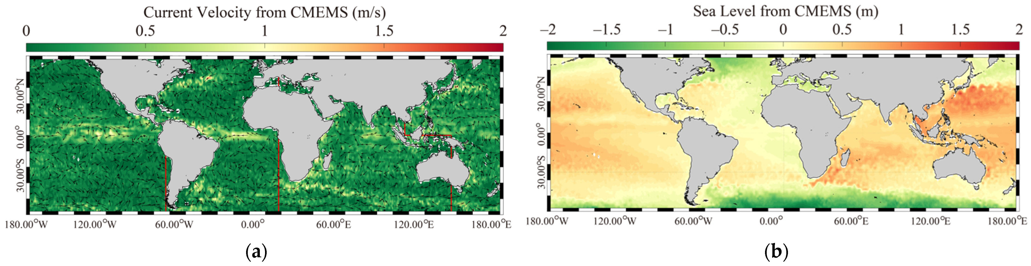
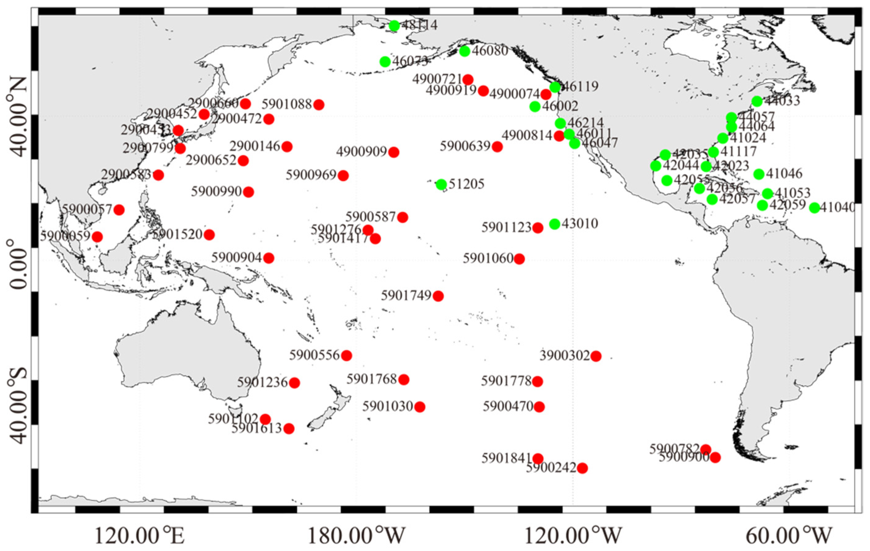
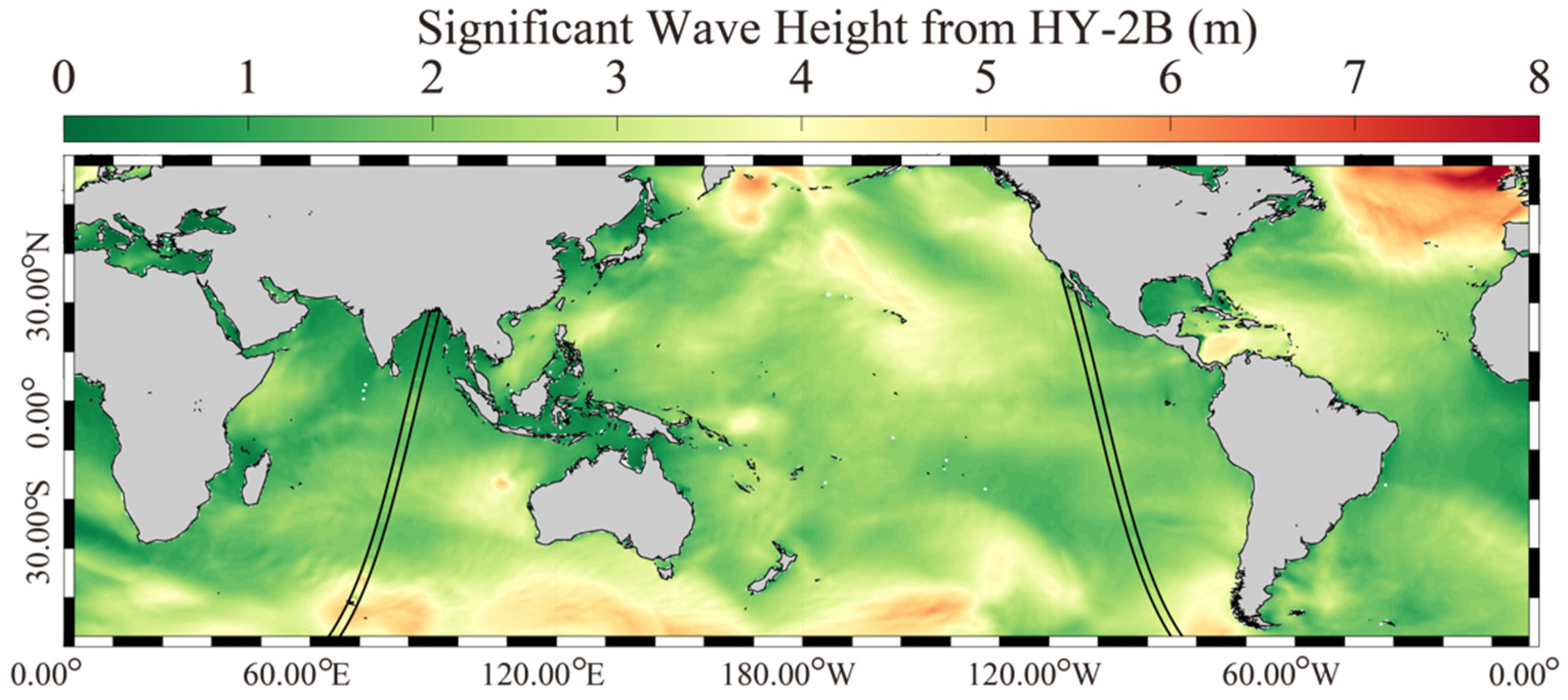
As examples, the maps of current velocity and sea level from CMEMS on 1 January 2020 are depicted in Figure 1a,b, in which the rectangles represent the boundary of the global ocean. The ERA-5 wind map at 00:00 UTC on 1 January 2020 is presented in Figure 1c. As for ensuring the applicability of WW3-simulated results, the observations from a few NDBC buoys are used, as represented by the green spots in Figure 2. Furthermore, the SWH measured from the Haiyang-2B (HY-2B) altimeter in 2020 are collected so as to validate the WW3 simulations. Figure 3 shows the measurements following the footprints of the HY-2B altimeter from 00:00 to 04:00 UTC on 15 January 2020.
2.2. Model Settings of sbPOM
As mentioned in Section 1, the basic principle of sbPOM is the same as that of POM, using the moment equation in the σ-coordinate:
wherein H(x,y) is the terrain at sea bottom in the spatial dimensions of x and y; η(x,y,t) is the magnitude at the sea surface (z = η) referred to the bottom (z = −H) in the directions x, y, and the time dimension t; u, v, and ω represent the component of speed. In the vertical dimension, the bottom-following σ ranges from −1 to 0, and has the formula:
Since 1990, the Simple Ocean Data Assimilation (SODA) dataset has been used, and it uses the global ocean data by assimilating the observations into numerical simulations; however, it has a relatively low spatial resolution (a 0.5° grid). The SODA SST and sea surface salinity based on a monthly average are set as the initial fields in the sbPOM modeling process. The land shore and the ocean bottom are adopted to be the solid wall boundaries according to a GEBCO water depth greater than 10 m. Moreover, the water depth is set at 5000 m, which is less than the maximum water depth in the SODA data. The total heat flux from NCEP data is calculated by:
in which Qe is the latent heat flux, Qh is the sensible heat flux, Qb is the long-wave radiation, and Qs is the solar radiation. The NCEP reanalysis dataset performs well on the relative strength of the synoptic-scale total heat flux forced over the long-term, which has been validated against with the measurements from moored buoys [53]. The 0.5° gridded ERA-5 winds at intervals of 6-h are set as the forcing field of the model. In particular, the four wave-induced terms, e.g., breaking waves, nonbreaking waves, radiation stress, and Stokes drift, calculated by wave parameters from WW3 model, are treated as the forcing field; these are described in [21] in detail, and we do not repeat these descriptions here. The NCEP flux field has a spatial resolution of 1.875° × 1.905° in the longitude × latitude direction at intervals of 6-h. The sbPOM utilizes a time split mode algorithm for the inner and outer modes [54]. Specifically, the outer mode is used for calculating the average current speed and water elevation; and the inner mode is used for calculating the parameters such as turbulent kinetic energy, three-dimensional current speed, temperature, and salinity. To ensure the stability of the sbPOM modelling, the time of the outer mode and the inner mode were set to be 20 and 600 s, respectively. Using available SODA data, the SST is simulated by sbPOM in 2005–2015 with a 0.2° spatial resolution and a 6-h temporal resolution. The settings for sbPOM are listed in Table 2.
Qt = Qs − Qb − Qe − Qh,
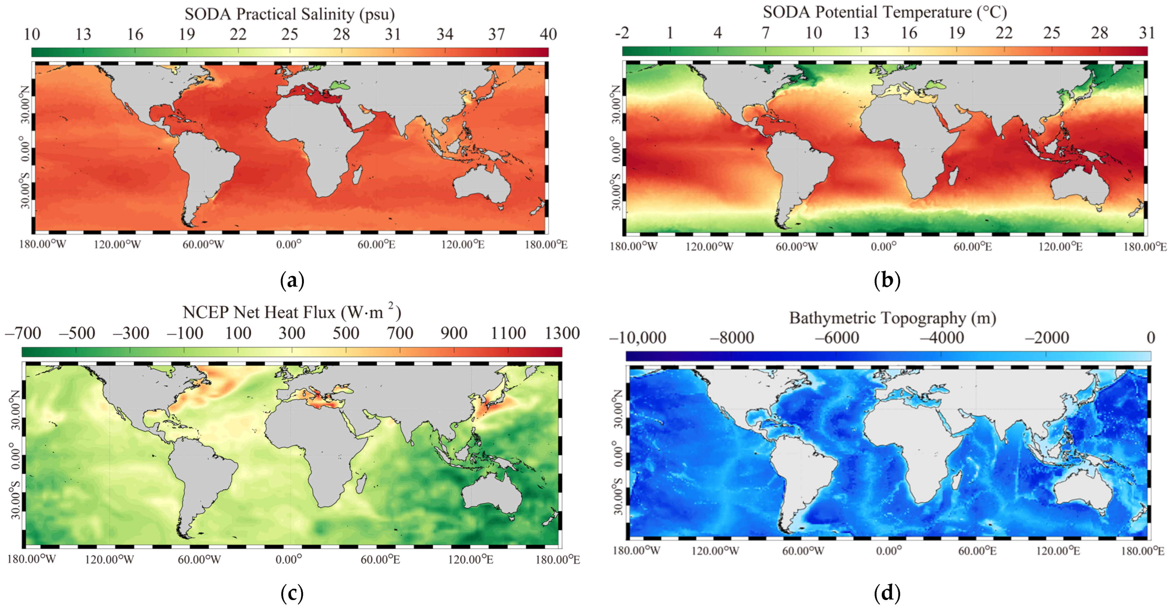
As an example, the maps of practical salinity and potential temperature from SODA on 1 January 2015 are presented in Figure 4a,b, respectively. Figure 4c shows the map of the NCEP heat flux on 1 January 2015.
Since 2000, a global project for constructing an array of temperature/salinity profiling floats, denoted as Argo, has been a well-calibrated source for ocean observation together with NDBC buoys. To confirm the accuracy of sbPOM-simulated water temperatures, the high-quality measurements from Argos were collected, and they are marked by red spots in Figure 2.
3. Results
The WW3-simulated SWHs are validated against the measurements from several NDBC buoys in 2020, and the sbPOM-simulated SSTs are compared with the Argos data in 2020. The inter-annual and seasonal variation of waves is analyzed. In particular, the inter-relations among SWH, current, and sea level are studied further.
3.1. The Validation of Model-Simulated Wave and sbPOM-Simulated Sea Surface Temperature
Using the WW3 model, the wave fields of global seas (60°S–60°N, 180°W–180°E) in 1993–2020 were simulated. To confirm the applicability of modelling results, the available SWHs measurements from more than 80 NDBC buoys were collected, which are illustrated as green points in Figure 2. As shown in Figure 5a,b, the statistical analysis yielded a root mean square error (RMSE) of 0.49 m with a correlation (COR) of 0.89 compared with NDBC buoys and an RMSE of 0.63 m with a COR 0.90 compared with HY-2B measurements, indicating a reliable accuracy of WW3-simulated waves.
Similarly, the SST was simulated by the sbPOM for the global sea (60°S–60°N, 180°W–180°E) in 2005–2015, which were statistically analyzed by comparison with more than 50 Argo datapoints from the Pacific Ocean. There was an RMSE of 1.12 °C and a COR of 0.99 between the sbPOM-simulated SST and the Argo buoys measurements (Figure 5c). Therefore, we believe that the SST simulated by sbPOM is reliable for use in this study.
3.2. The Interrelation between SWH and Current
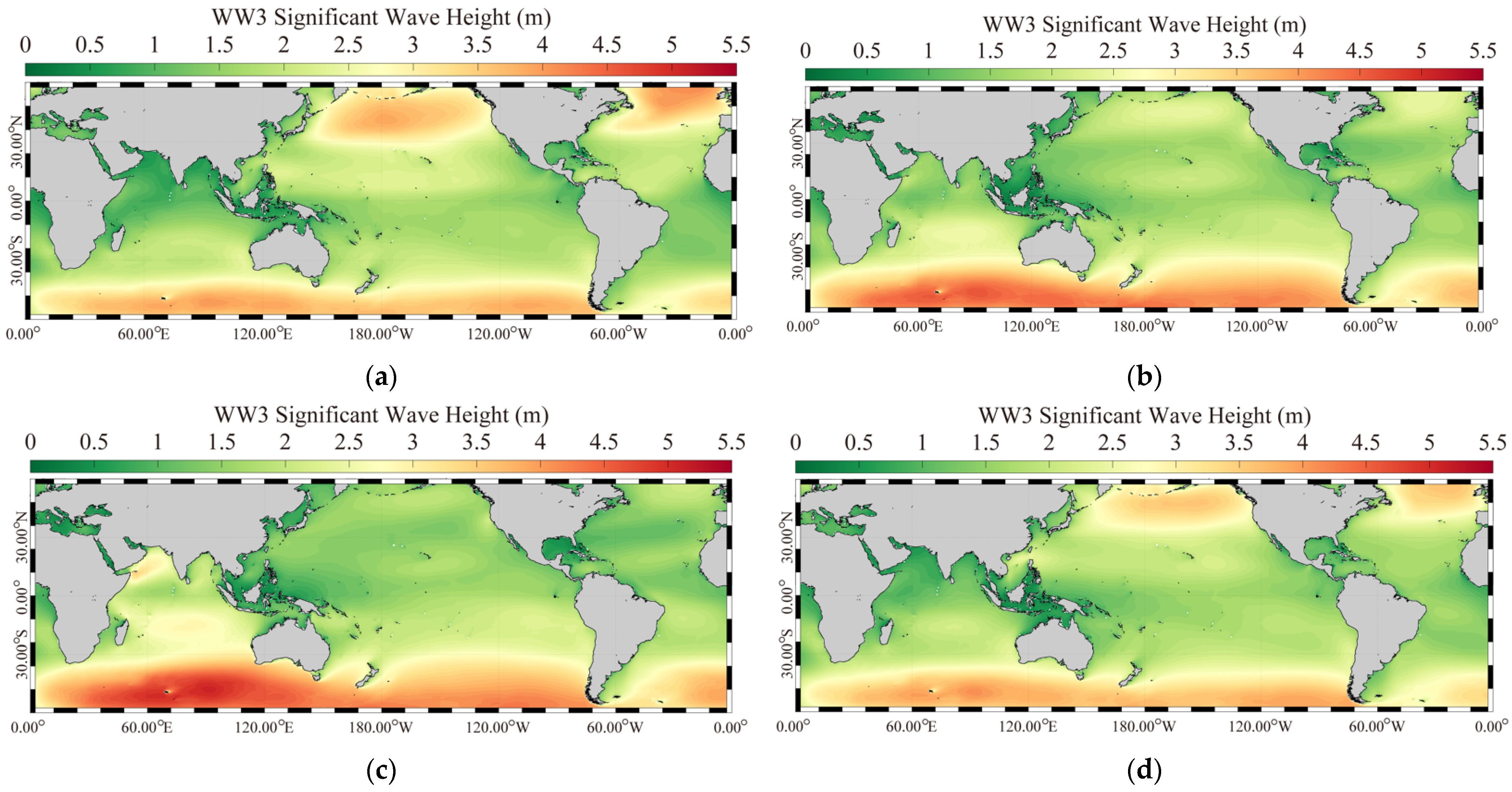
The seasonal-averaged WW3-simulated SWHs in 1993–2020 are shown in Figure 6: (a) spring; (b) summer; (c) autumn; (d) winter. In the equatorial areas of the Pacific Ocean and Atlantic Ocean, the SWHs were relatively high and were increased in summer and autumn. In the Indian Ocean, there exists a clear seasonal variation where the SWHs was low in spring and winter and gradually increased in summer and autumn. In the high latitudes of the northern hemisphere, the SWHs decreased in the summer and autumn, while SWHs increased in the spring and winter. However, the situation was contrasted in the southern hemisphere.
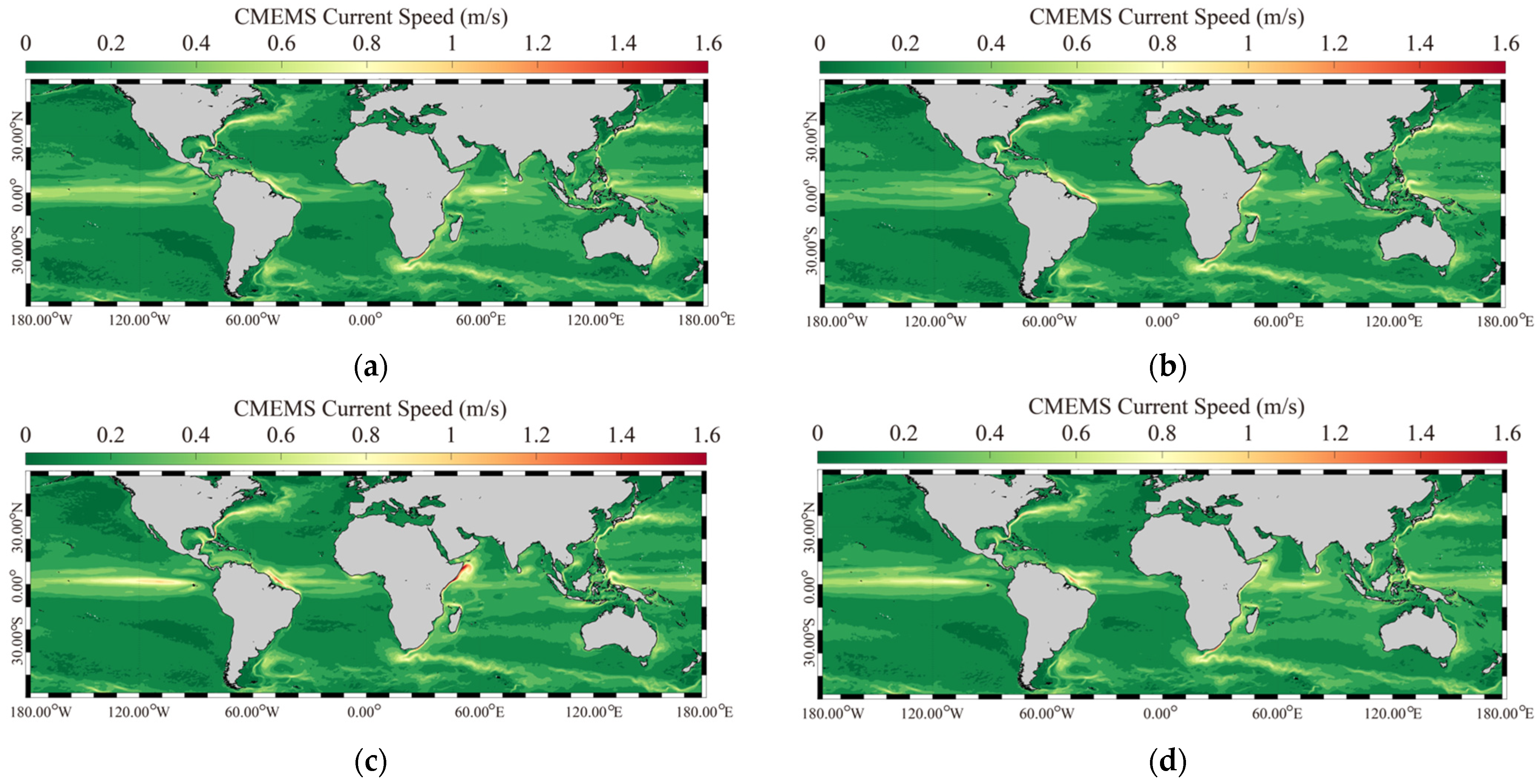
The seasonal-averaged CMEMS currents in 1993–2020 are shown in Figure 7. The seasonal variation of the current speed in some areas where the surface circulation flows can be easily observed. In the Pacific Ocean, the equatorial currents were weak in the summer. In the Atlantic Ocean and the Indian Ocean, the currents in the area where the southern equatorial warm current and the Somali warm current flow were strong in autumn. Compared with the seasonal change of the current and the SWHs, the inter-relation of the two oceanic parameters was strong in the Indian Ocean. In the other two ocean areas, the inter-relations were not as clear.
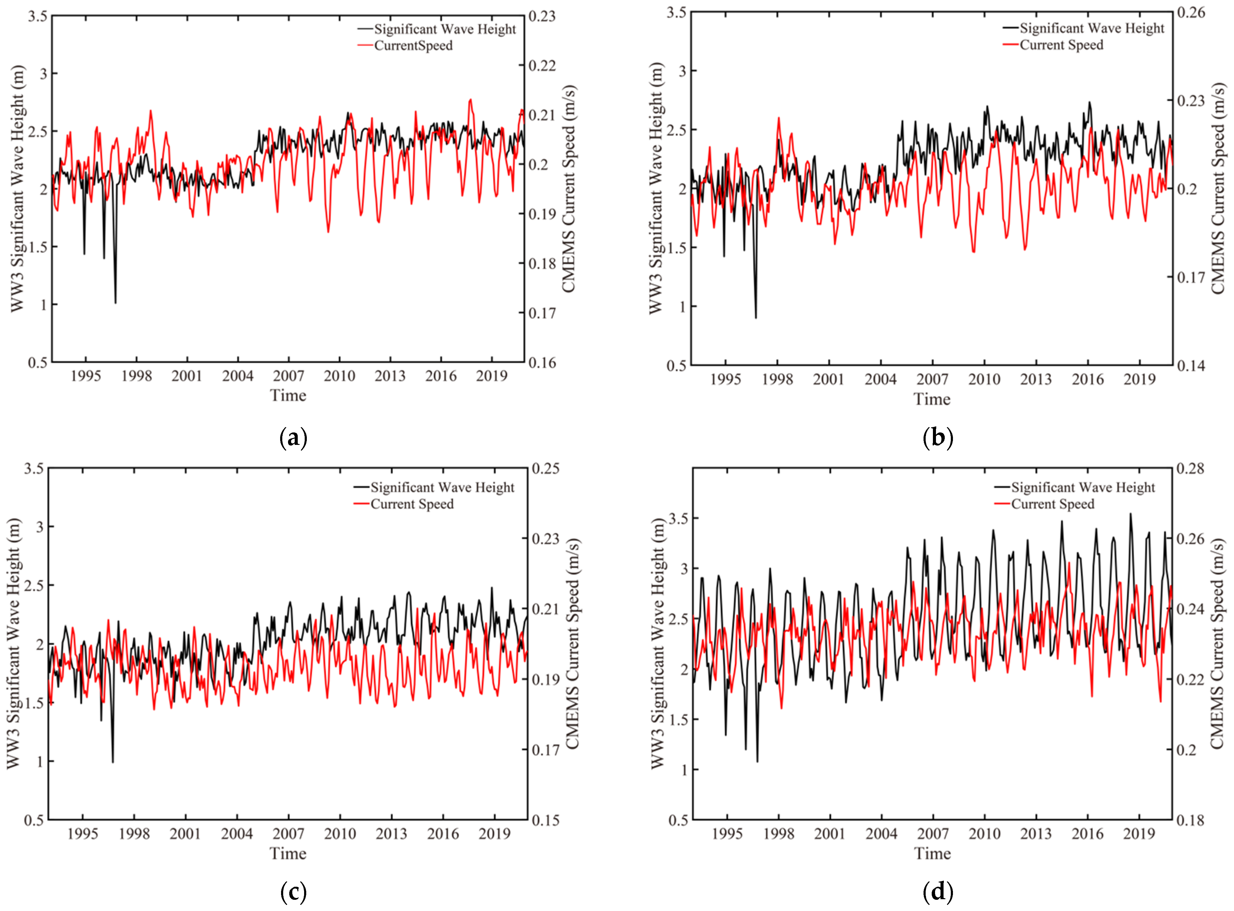
The comparisons of the WW3-simulated SWHs and the CMEMS current speed in the global seas (a) the Pacific Ocean, (b), the Atlantic Ocean, (c) and the Indian Ocean, (d) are shown in Figure 8. The dividing lines of the Pacific Ocean, Atlantic Ocean, and Indian Ocean are shown as red solid lines in Figure 1a. In 1993–2012, the monthly variation trend of the SWHs was gradually increased in the global seas and the three ocean areas. Specifically, as shown in Figure 8d, the oscillations of the SWHs and the current speed were consistent in the Indian Ocean during the past 28 years.
3.3. The Relationships among SWH, Sea Level, and Sea Level Anomaly
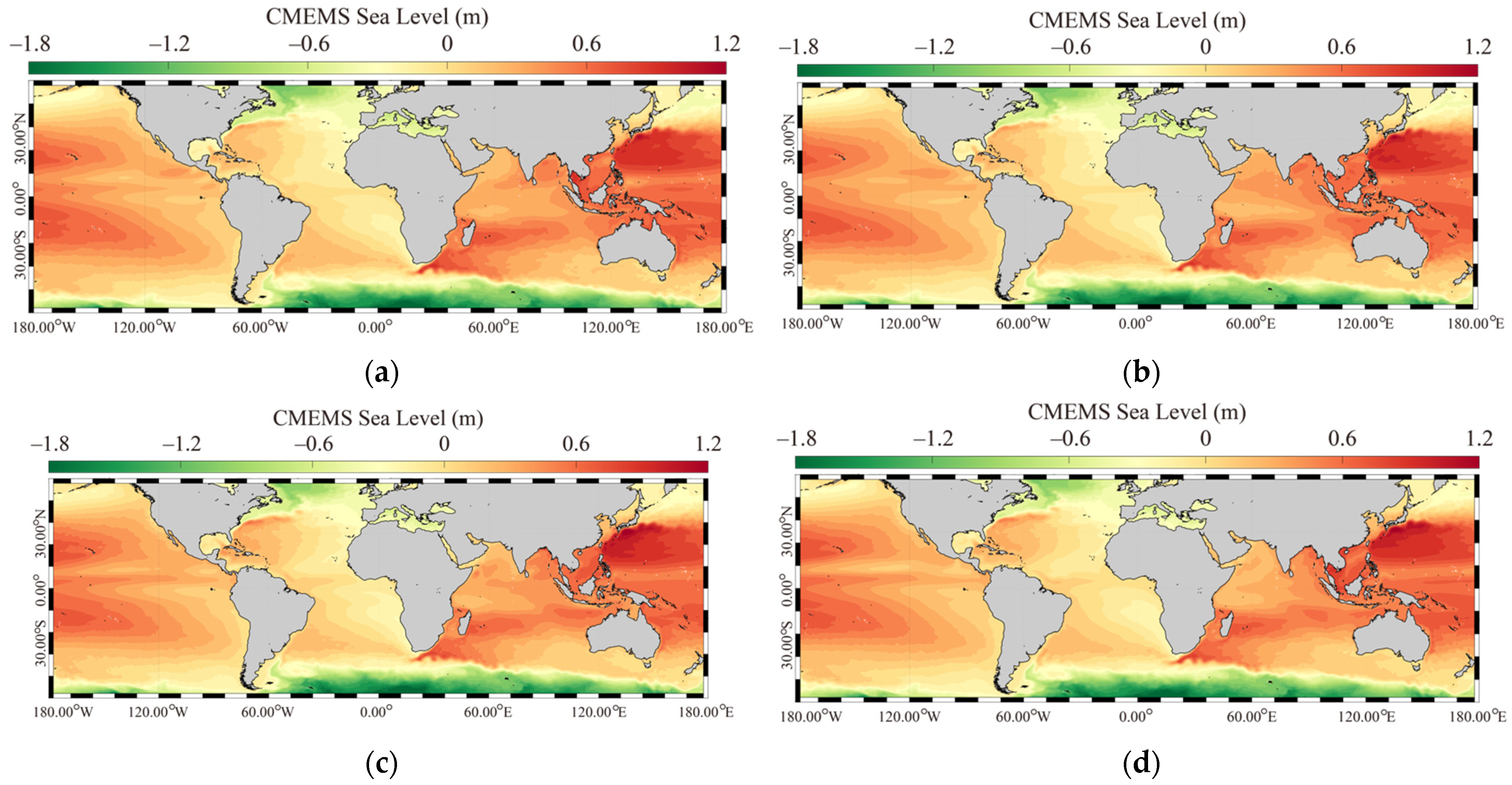
The seasonal-averaged CMEMS sea level is shown in Figure 9. The sea surface elevation was always high at the lower latitudes of the three oceans, but low at the higher latitudes of the three oceans. Compared with the global SWHs shown in Figure 6, the distribution of the sea level was consistent with the SWHs in the strong current areas such as equatorial circulation and Kuroshio, where both parameters increased. In the global sea, the seasonal variation of currents was not evident in the past 28 years.
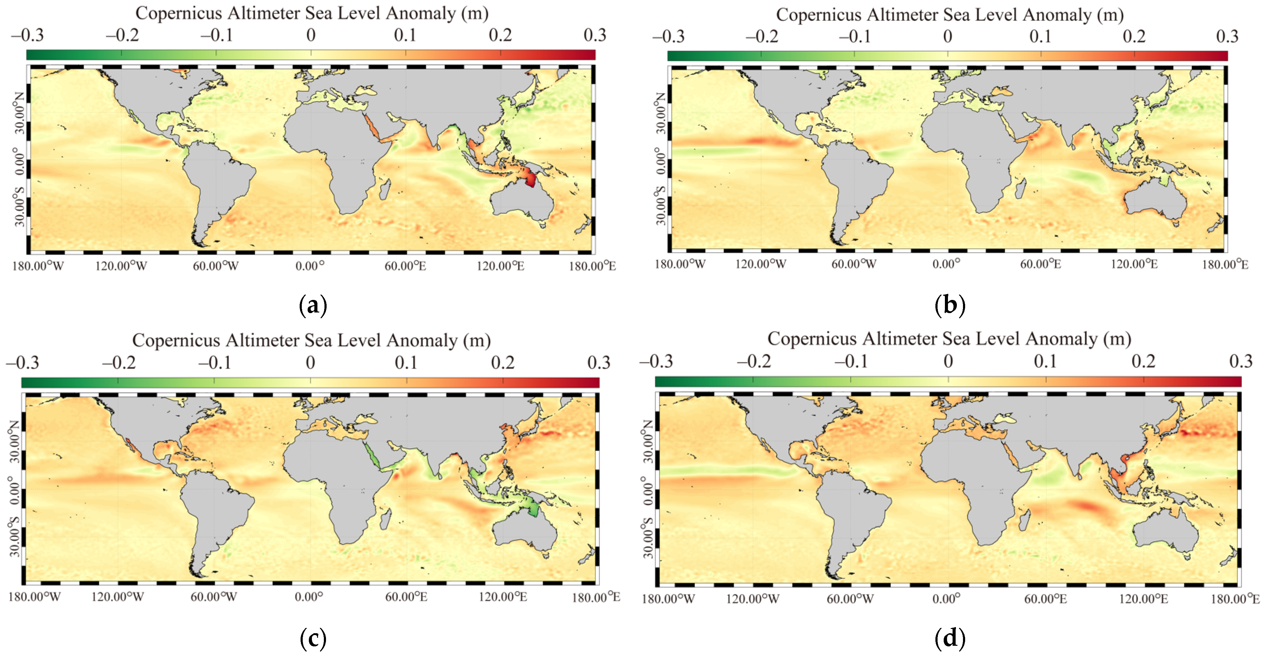
The global seasonal-averaged sea level anomaly from the CMEMS [55] is shown in Figure 10. The sea level anomaly rose in the southern hemisphere and fell in the northern hemisphere in spring and summer. In autumn and winter, the sea level anomaly rose in the northern hemisphere and fell in the southern hemisphere. However, in the equatorial ocean areas, the seasonal variation was the opposite.
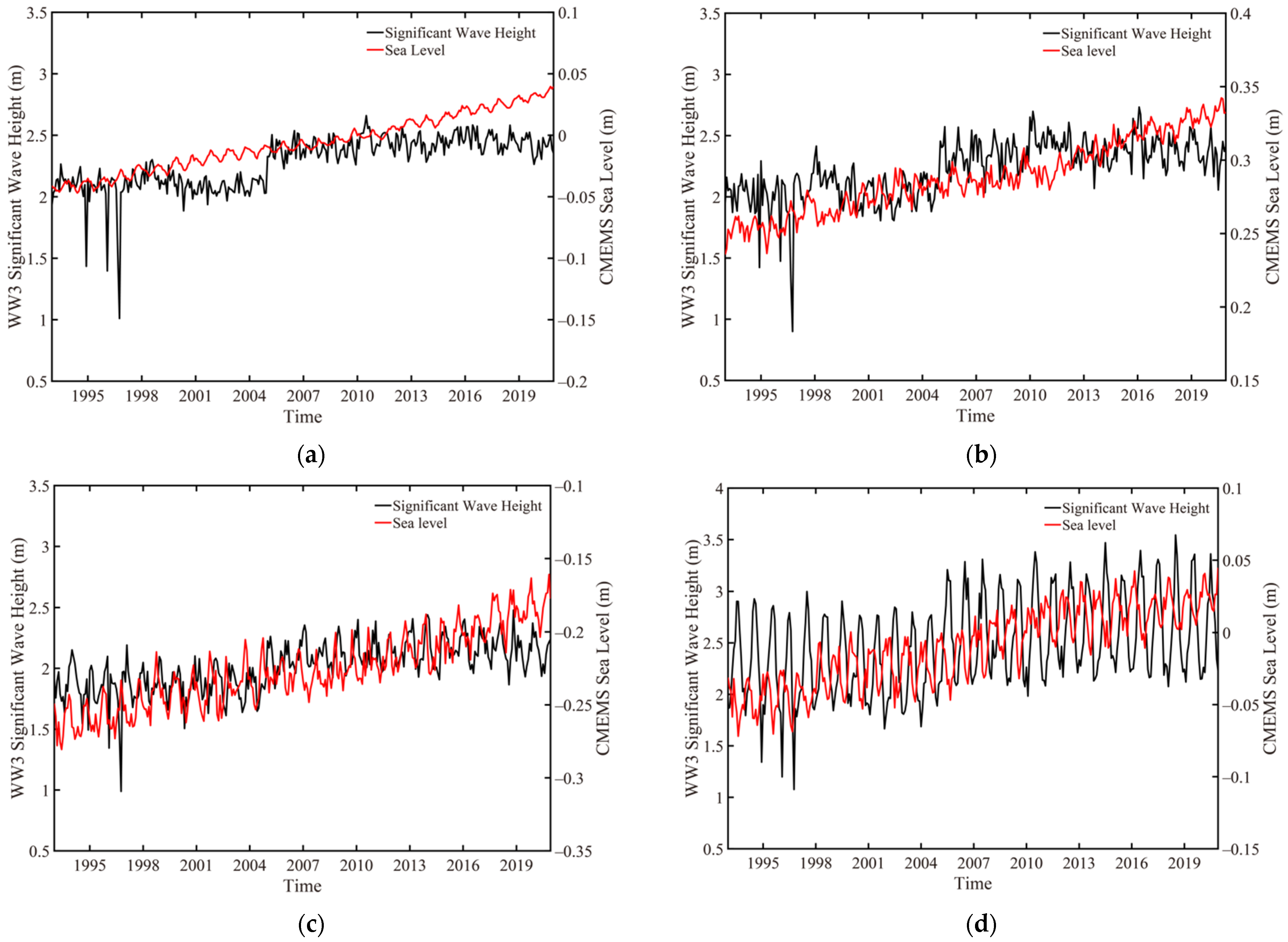
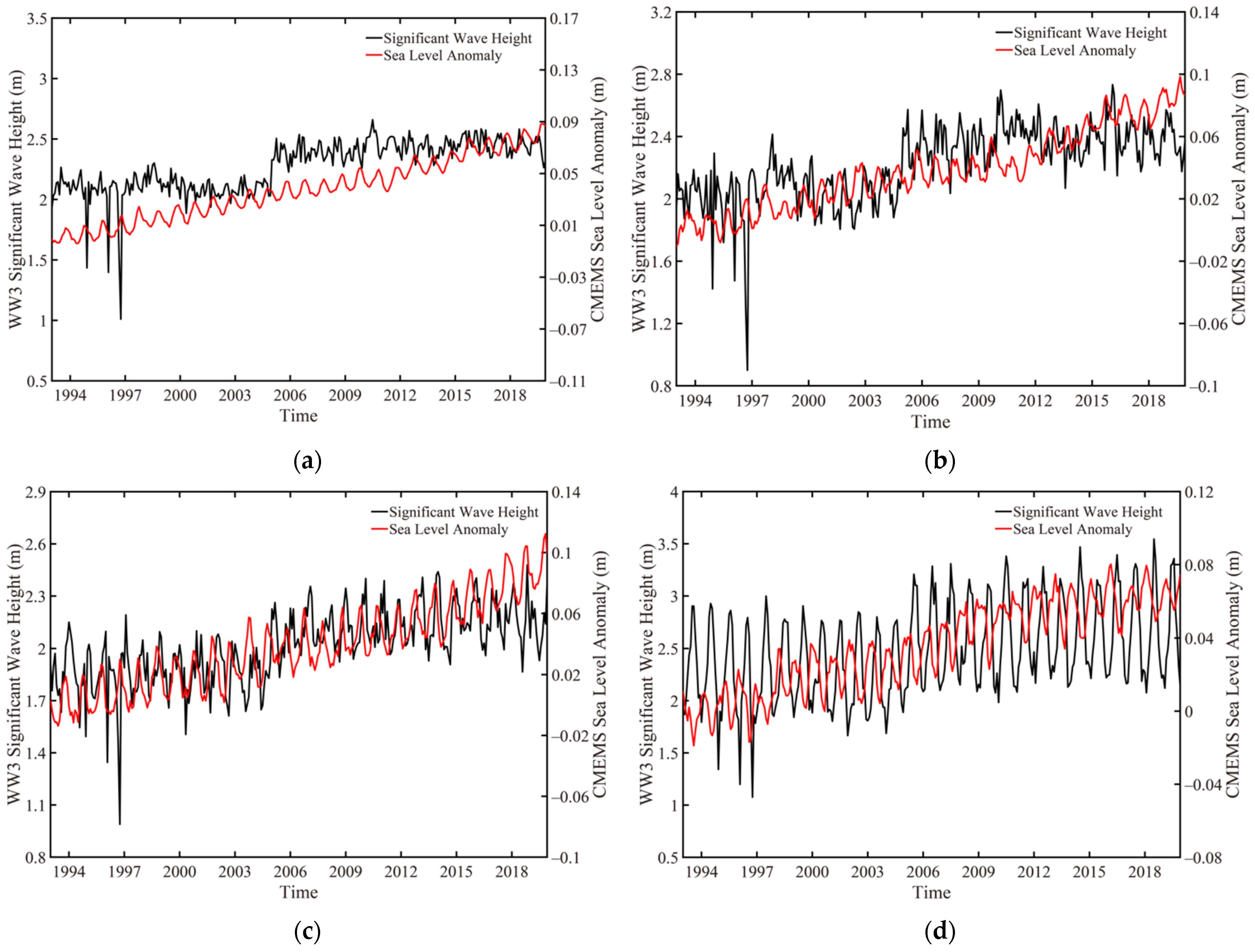
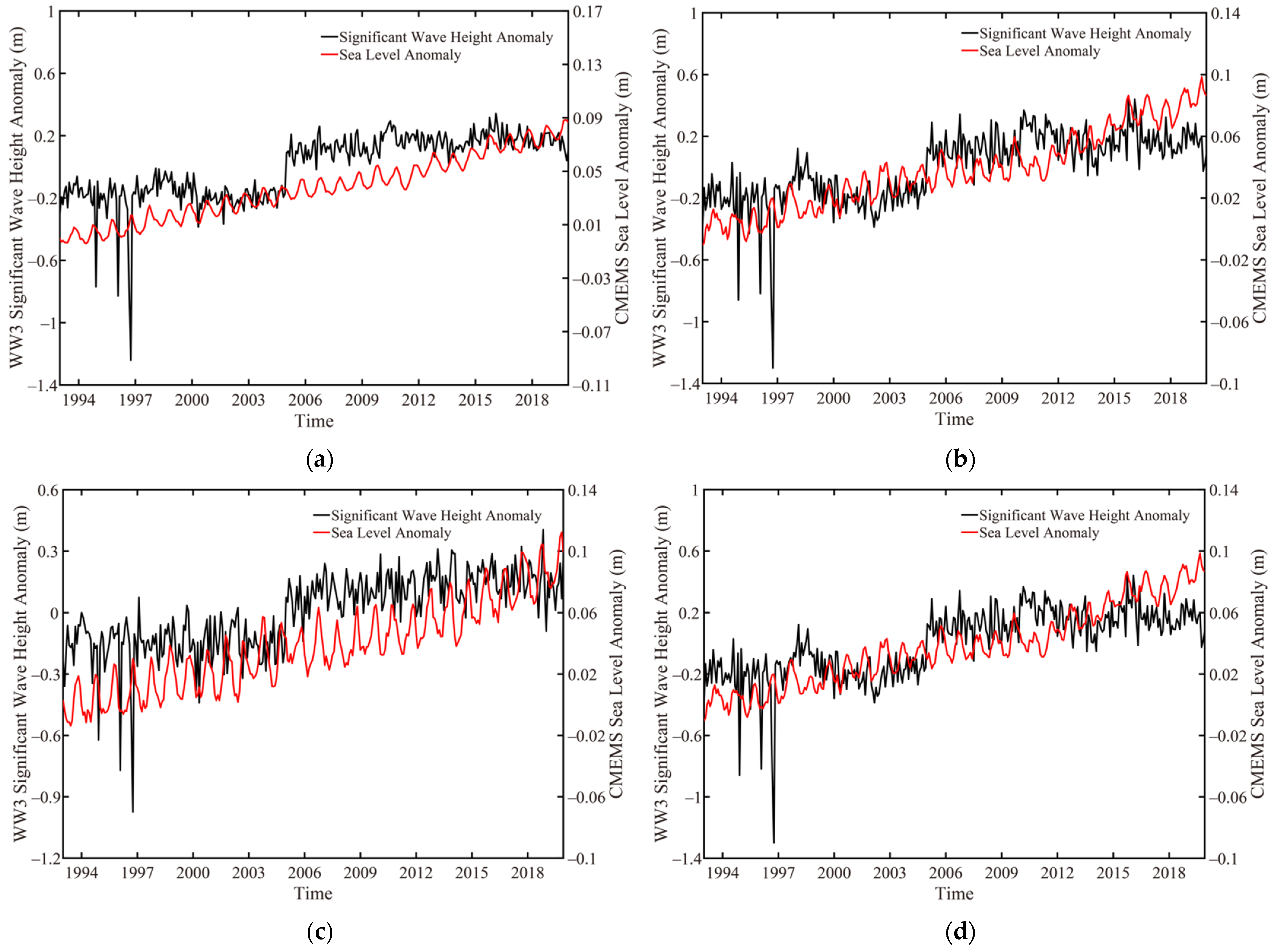
Comparing the monthly-averaged WW3-simulated SWHs, the WW3-simulated SWHs anomaly, the CMEMS sea level, the CMEMS sea level anomaly in the global seas, and the Pacific Ocean, Atlantic Ocean, and Indian Ocean during the past 28 years, the relationship among the SWHs, sea surface elevation, and sea level anomaly was analyzed. As shown in Figure 11, Figure 12 and Figure 13, the upward trends of the monthly SWHs, sea level and the sea level anomaly were consistent in 1993–2015 in the three oceans. However, the upward trend of the SWHs slowed down between 2015–2021.
3.4. The Relationships among SWH, SST and Sea Surface Wind Stress
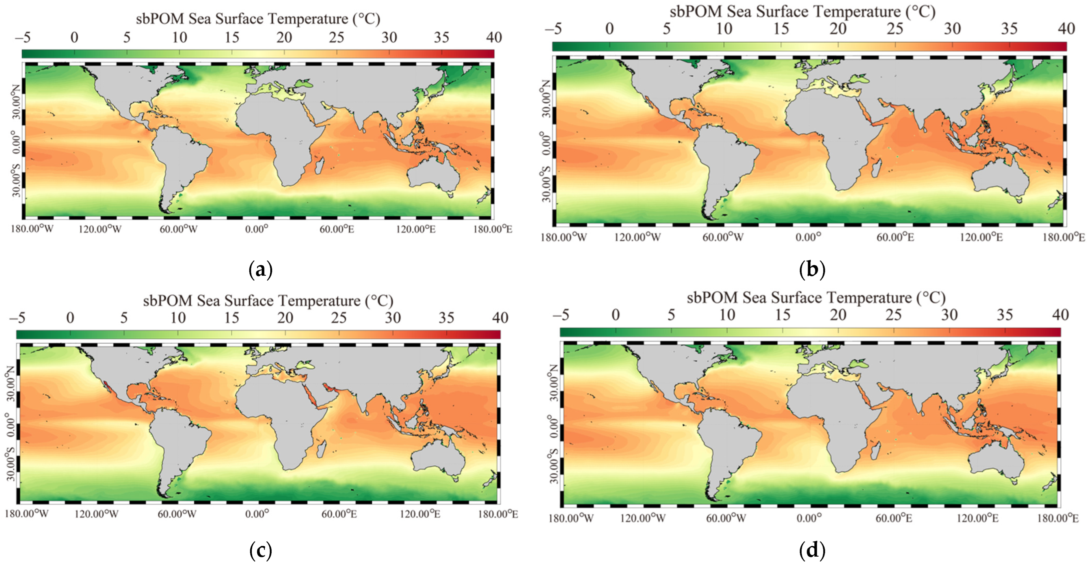
As mentioned in [52], the four terms induced by waves contribute to the ocean circulation; therefore, it is essential to analyze the influence of water temperature on waves. The seasonal-averaged sbPOM SST in 1993–2015 is shown in Figure 14. In general, the SST in the equatorial areas and western boundary of the Pacific Ocean and the Atlantic Ocean was cold, especially in autumn and winter. At the eastern boundary of the Indian Ocean, the low SST appeared in autumn. The SST in the high-latitude areas was cold and became warm in the low-latitude areas. This latitude-distribution is governed by the declination of the sun.
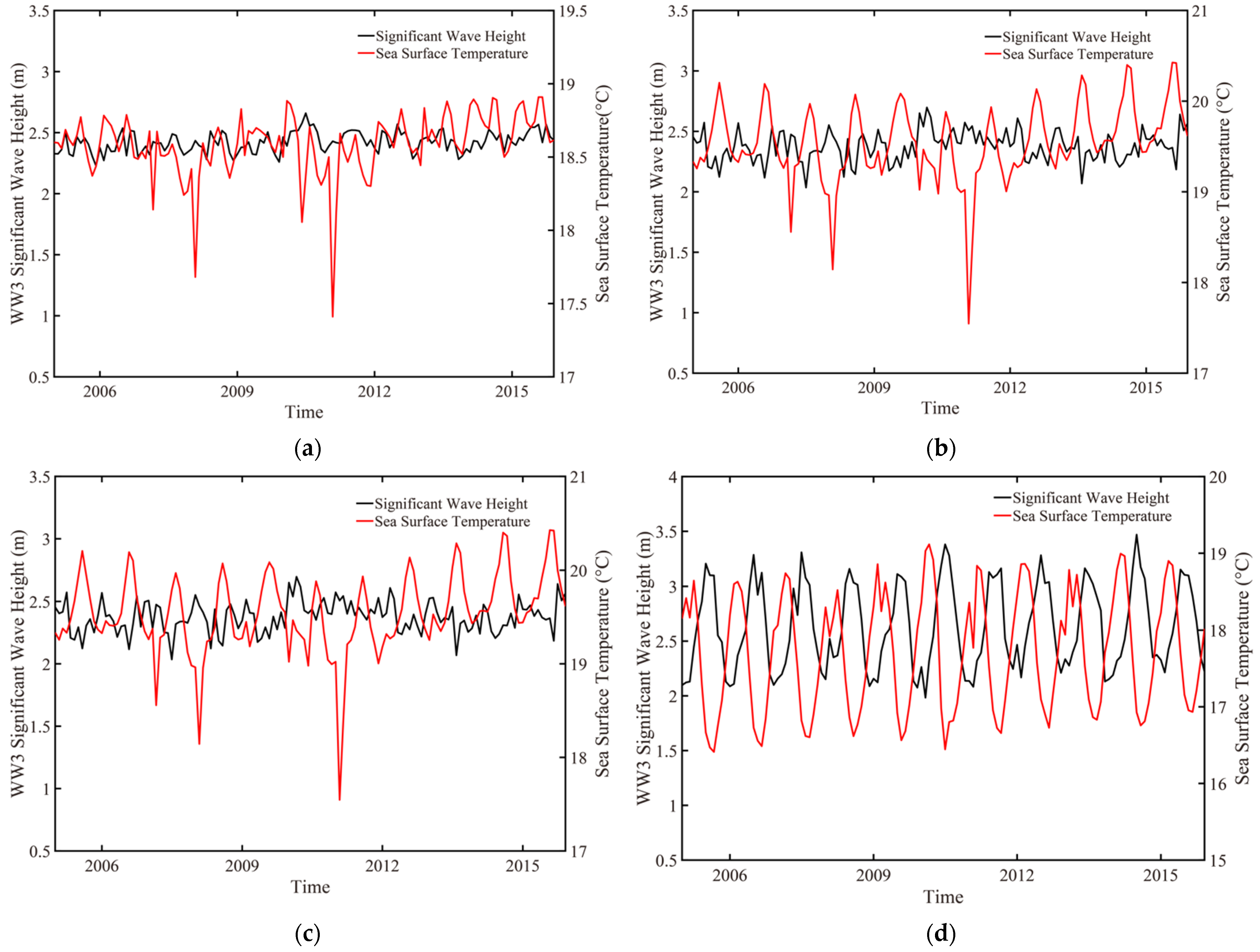
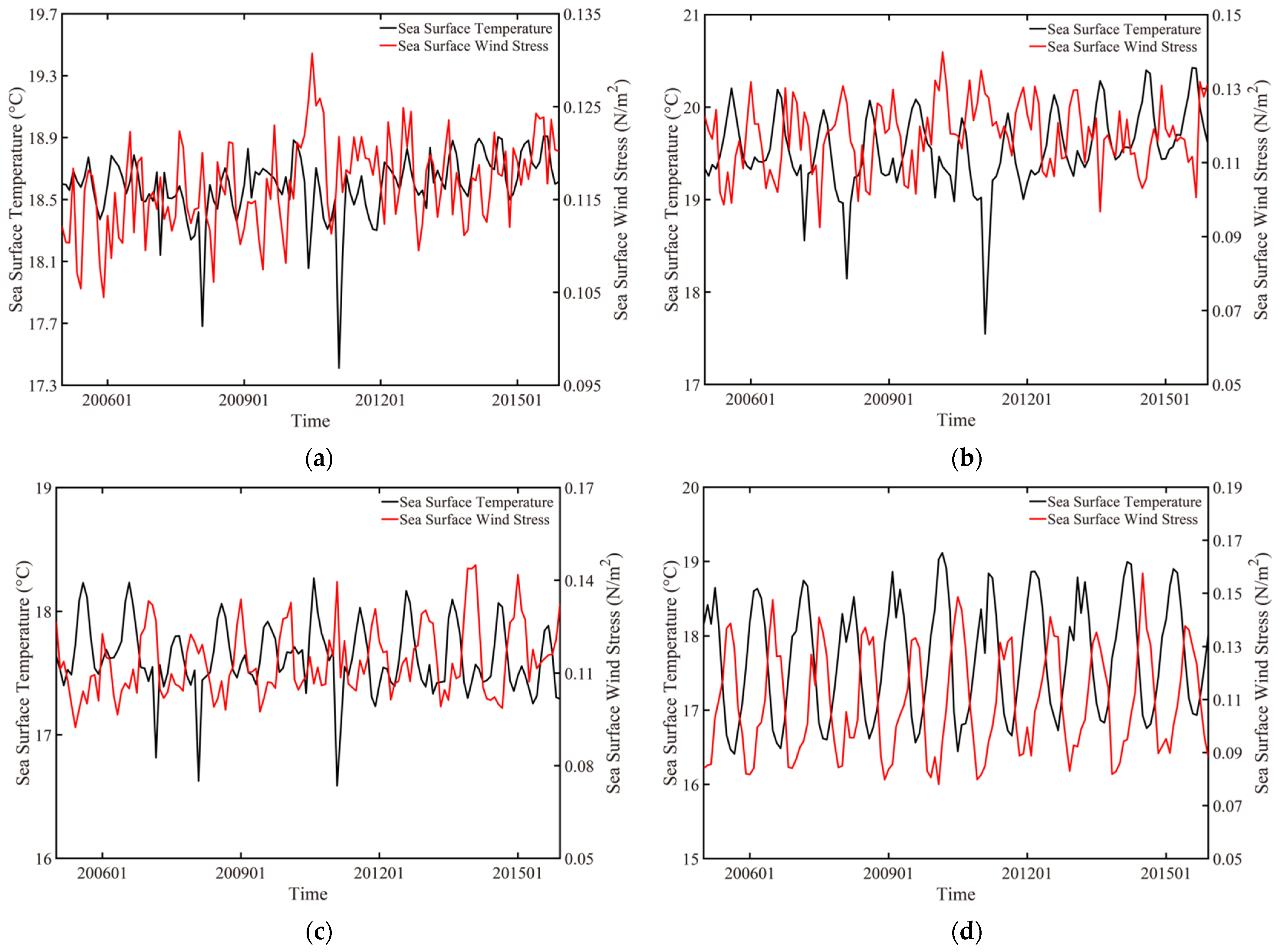
To analyze the relationship between the monthly-averaged SWHs and SST, the comparisons of the WW3-simulated SWHs and the sbPOM-simulated SST in the global ocean, the Pacific Ocean, the Atlantic Ocean, and the Indian Ocean are shown in Figure 15. During the past 10 years, the SST oscillation had a passive response to the SWHs in the three oceans that revealed a strong correlation between the SST and SWHs. In addition, the globally monthly-averaged SST increased from 2012, while the SWHs presented a trend that was similar to that of the Pacific Ocean, as illustrated in Figure 15b. Otherwise, the ocean waves were driven by winds. In order to analyze the influence of winds on SWHs and SST, the monthly-averaged sea surface wind stress was compared to the SST and SWHs, as illustrated in Figure 16 and Figure 17, respectively. The sea surface wind stress (τ) calculation equation is:
in which ρa represents the sea surface air density, U10 is the 10-m wind above sea surface, and Cd is the sea surface drag coefficient, which was calculated by an empirical function [20],
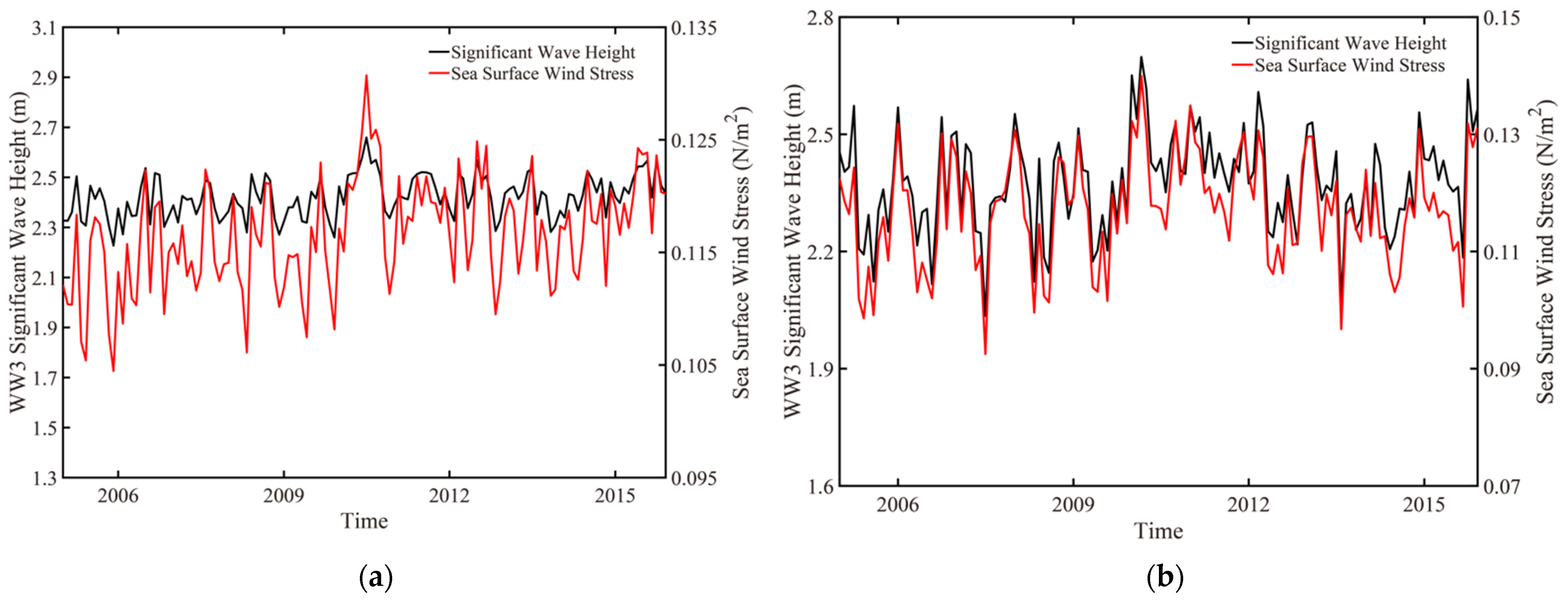
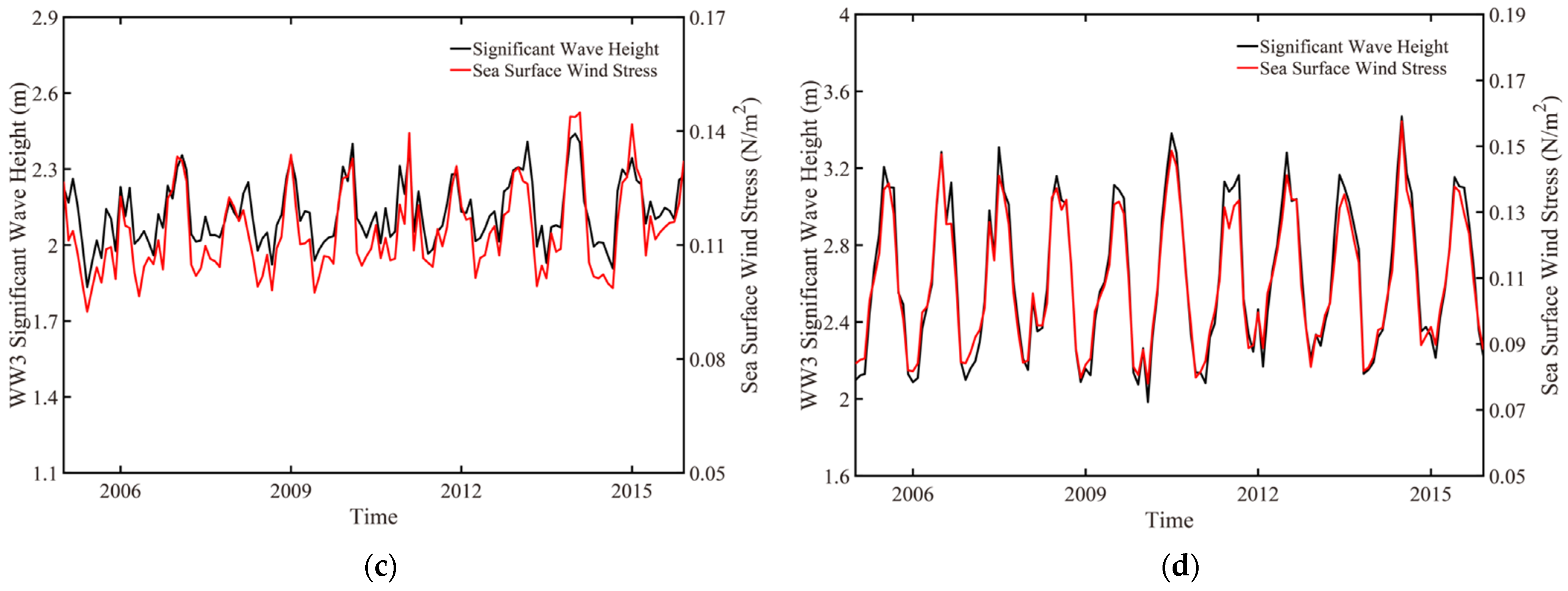
Against the background of global climate change, both SST and wind stress gradually increased from 2005–2015, as shown in Figure 16 and Figure 17. The interrelation between the sea surface wind stress and the SST was similar to the relationship between the SWHs and the SST, which both presented a passive oscillation during the past 10 years. The SWHs and the sea surface wind stress presents a positive correlation in the three oceans, which is consistent with previous studies. In particular, comparing the SST and the SWHs, the annual distributions were opposite in the three oceans, especially for the Indian Ocean. In this sense, the influence of waves on SST should be further discussed.
4. Discussion
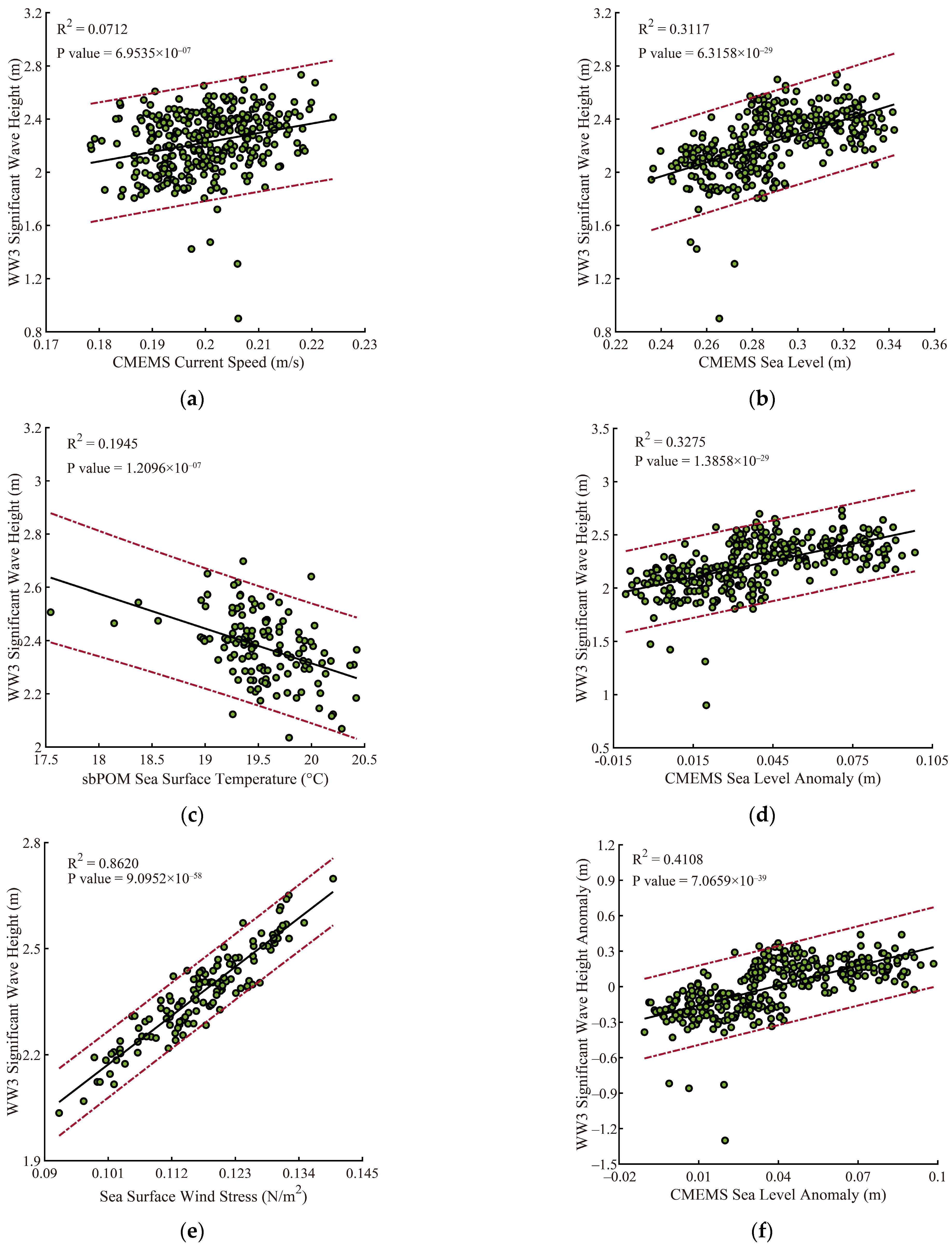
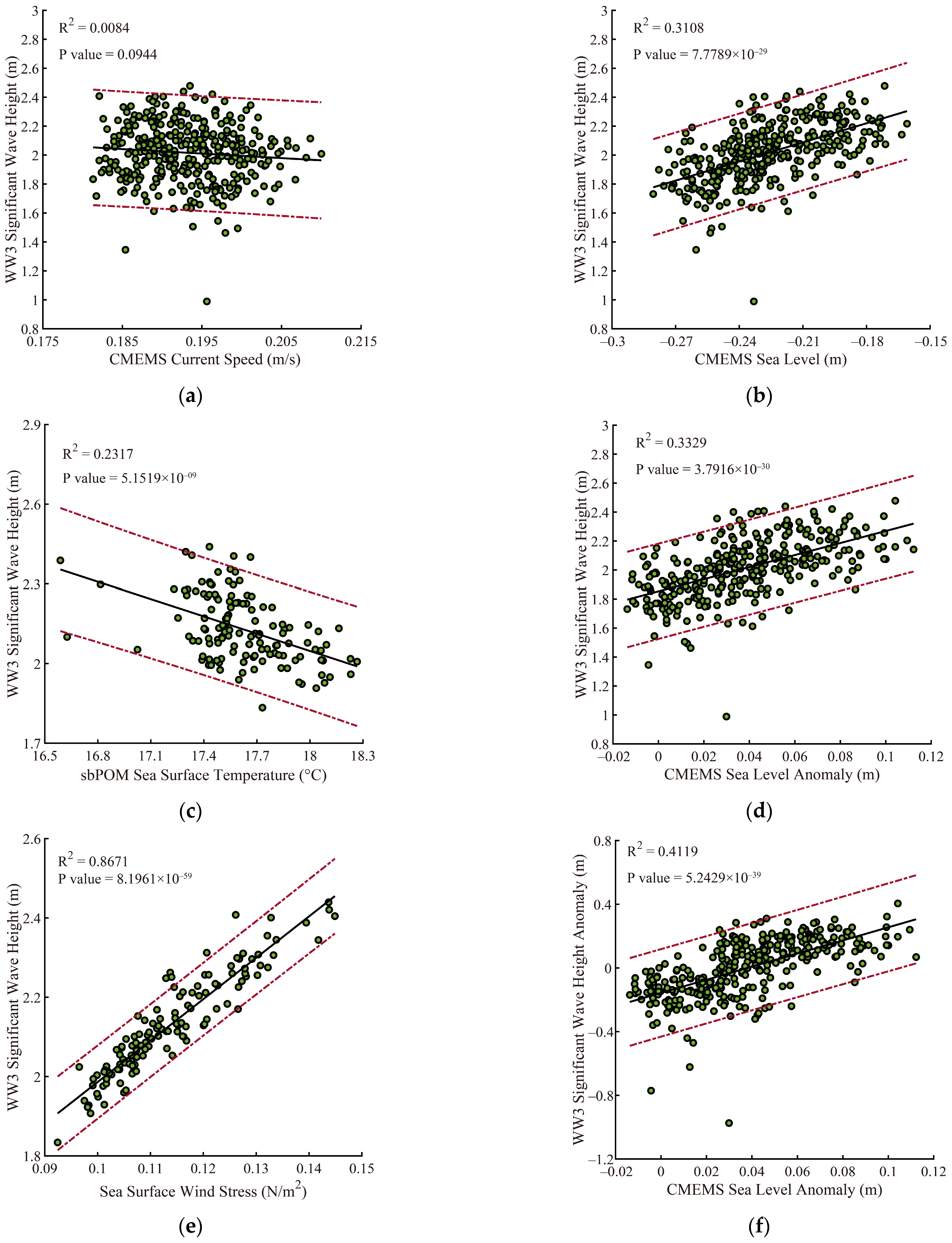
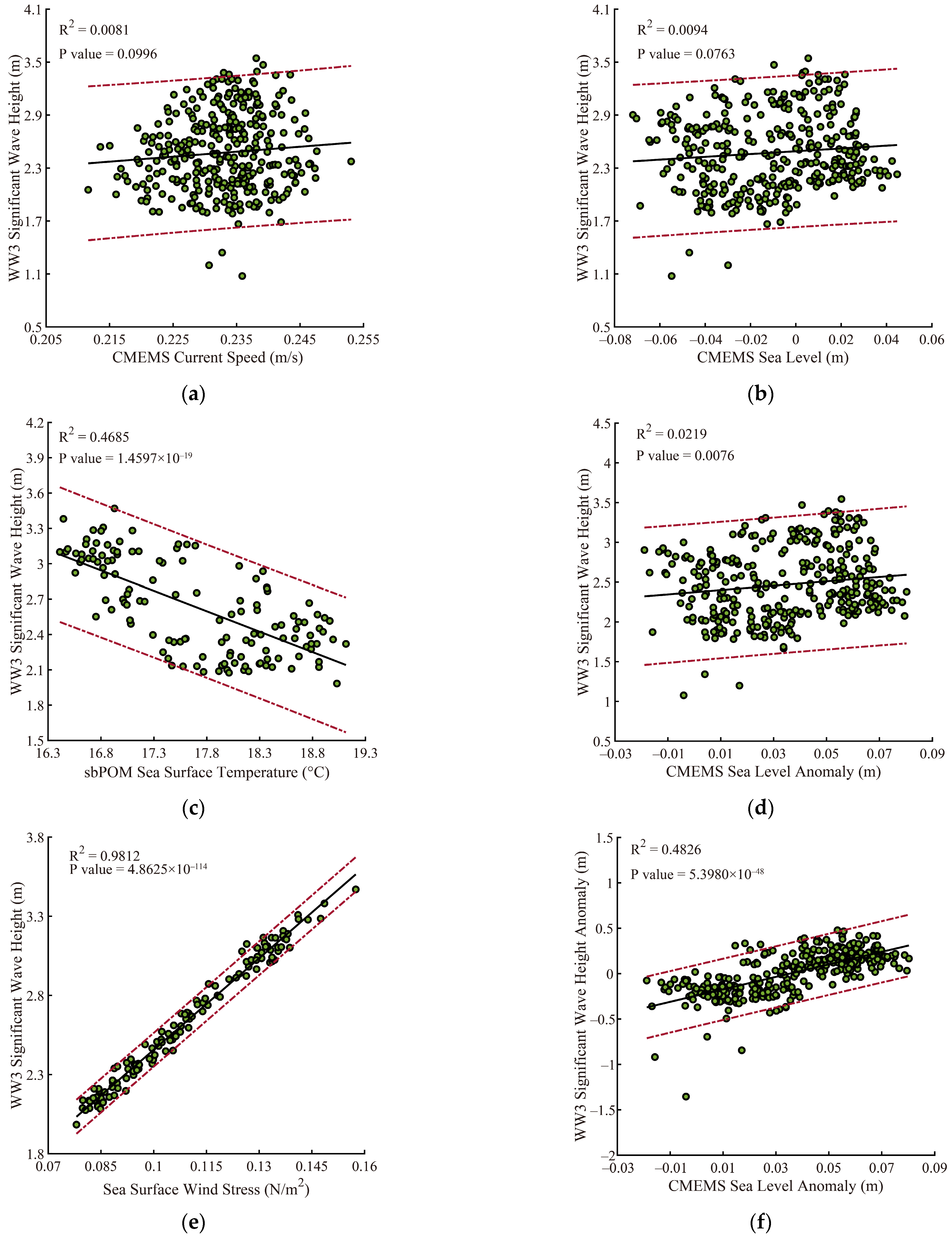
To analyze the influence of the five marine parameters (current, sea surface elevation, SST, sea level anomaly and sea surface wind stress) to the SWHs quantitatively in the three oceans, a linear regression analysis was used. As illustrated in Figure 18, Figure 19 and Figure 20, a significant positive correlation between the SWHs and sea surface wind stress in the Pacific Ocean, the Atlantic Ocean and the Indian Ocean was observed, in which the square of CORs (R2 > 0.8) was larger than the other parameters (current, SST, sea surface elevation and sea level anomaly). This is because the ocean waves were induced by the winds, and the waves increased with the increasing of the sea surface wind stress. However, the SST has a negative correlation with the SWHs (R2 > 0.2) because the growth of waves should dissipate energy and reduce the temperature at the air–sea layer. Furthermore, the SWH anomaly and the SWH had a positive effect on the CMEMS sea level and sea level anomaly (R2 > 0.3) in the Pacific Ocean and the Atlantic Ocean, indicating that the rise of sea level also could enlarge the strength of wave over the long-term. In the Indian Ocean, the influence of SST and sea surface wind stress to the SWHs were more obvious, while, conversely, the influence of sea level and sea level anomaly weakened. We think the effect induced by the Arctic Ocean was weak, because the Indian Ocean only connects to the Southern Ocean. Otherwise, the Indian Ocean monsoon also contributed to the negative correlation in the Indian Ocean, which strengthens the sea surface heat flux. The CMEMS currents had no such significant effects on the SWHs in the three oceans (R2 < 0.1). From the perspective of climate change, the enhancement of waves could slow down the amplitude of water warming.
5. Conclusions
With the rapid melting of the sea ice in the Arctic and Antarctic Oceans [56], the rise of the global sea level has been observed by long-term satellites and moored buoys [57]. Recent studies have focused on the distribution of waves in regional seas and tropical cyclones using numerical models. As concluded in [6], the accuracy of wave simulations by numeric models is improved in tropical cyclones considering the influence of currents. In the background of climate change (i.e., the rise in sea levels), the terms of current and sea level are included in the wave simulations. Moreover, the water temperature of the upper layer is affected by waves. Therefore, this work studied the variation of the global wave distribution and its effect on SST in the background of climate change.
In this study, WW3 and sbPOM were employed to simulate the sea surface waves for the period of 1993–2020 and SST for the period of 2005–2015. The WW3-simulated SWHs were statistically validated by comparison with the measurements obtained from the NDBC buoys, yielding a better RMSE of 0.49 m with a better COR of 0.89 than the results (i.e., 0.63 m RMSE) compared with the HY-2B altimeter. Four wave-induced terms: breaking waves, nonbreaking waves, radiation stress, and Stokes drift, that were calculated by wave parameters from WW3 model, were included in the SST simulation by the sbPOM. The validation of the simulated water temperature was statistically analyzed by comparison with the Argo buoys, yielding a RMSE of <1.2 °C with a COR of >0.95.
In the qualitative analysis, the annual variation of SWH is consistent with that of CMEMS currents and CMEMS sea level, indicating that the current has an inevitable influence on wave simulations in the WW3 model. With the increasing CMEMS sea level and sea level anomaly, the monthly-average SWHs increased in the period of 1993–2020, where it was strong in the Pacific Atlantic Oceans but weak in the Indian Ocean. In other words, the growth of waves was in accordance with the rise of sea levels in the past 28 years. Furthermore, the regression among globally monthly-averaged SWH, sea surface wind stress, and SST were analyzed, finding that SWH is positively determined by sea surface wind stress in global oceans (R2 > 0.8). In addition, the sea level anomaly and the SWH presented a positive correlation in the Pacific and Atlantic Oceans (R2 > 0.3). Interestingly, the SST oscillation had a negative response to the SWH (R2 > 0.2). This behavior was clearly observed in the Indian Ocean due to the Indian monsoon and the lack of a connection with the Arctic Ocean.
In summary, the following conclusions can be drawn: with climate change, the wind stress intensity and sea level increase, which enhances the growth of waves; the wave-induced factors strengthen the heat exchange at air–sea layer, resulting in the negative relationship between SWH and SST. It is assumed that the growth of waves could weaken the water warming, especially in the Arctic [56] and Antarctic Oceans [40], which will be studied in the future.
Author Contributions
Conceptualization, W.S. and R.Y.; methodology, W.S. and R.Y.; validation, R.Y.; formal analysis, W.S., S.H. and J.Z.; investigation, R.Y., M.H. and S.H.; resources, W.S.; writing—original draft preparation, W.S., M.H., J.Z. and R.Y.; writing—review and editing, W.S., and S.H.; visualization, R.Y. and W.S.; funding acquisition, W.S. and J.Z. All authors have read and agreed to the published version of the manuscript.
Funding
This research was funded by the National Natural Science Foundation of China under contract nos. 42076238, 42176012, and 42130402, the National Key Research and Development Program of China under contract no. 2021YFC3101702, the Natural Science Foundation of Shanghai under contract no. 23ZR1426900, and the 2023 Undergraduate Innovation and Entrepreneurship Training Program of the Shanghai Ocean University under contract no. X202310264028.
Data Availability Statement
Due to the nature of this research, the participants of this study did not agree to their data being shared publicly; therefore, the supporting data are not available.
Acknowledgments
We appreciate the provision of the WAVEWATCH-III (WW3) model developed by the National Oceanic and Atmospheric Administration (NOAA). The original code of the Stony Brook Parallel Ocean Model (sbPOM) can be accessed at http://www.ccpo.odu.edu (accessed on 2 April 2023). The European Centre for Medium-Range Weather Forecasts (ECMWF) wind field is available at http://www.ecmwf.int (accessed on 2 April 2023). The General Bathymetry Chart of the Oceans (GEBCO) water depth can be accessed via ftp.edcftp.cr.usgs.gov (accessed on 2 April 2023). The National Centers for Environmental Prediction (NCEP) wind field and heat flux data can be accessed via http://www.cdc.noaa.gov (accessed on 2 April 2023). The measurements from the National Data Buoy Center (NDBC) buoys of NOAA can be collected via http://www.ndbc.noaa.gov (accessed on 2 April 2023). The sea current, sea level and sea level anomaly data from the Copernicus Marine Environment Monitoring Service (CMEMS) can be accessed via https://marine.copernicus.eu (accessed on 2 April 2023).
Conflicts of Interest
The authors declare that there are no conflict of interest. The funders had no role in the design of the study; in the collection, analyses, and interpretation of the data; in the writing of the manuscript; or in the decision to publish the results.
References
- Rohling, E.J.; Grant, K.; Hemleben, C.; Siddall, M.; Hoogakker, B.; Bolshaw, M.; Kucera, M. High rates of sea-level rise during the last interglacial period. Nat. Geosci. 2008, 1, 38–42. [Google Scholar] [CrossRef]
- Thompson, B.; Gnanaseelan, C.; Parekh, A.; Salvekar, P.S. North Indian ocean warming and sea level rise in an OGCM. J. Earth Syst. Sci. 2008, 117, 169–178. [Google Scholar] [CrossRef]
- Proshutinsky, A.; Pavlov, V.; Bourke, R.H. Sea level rise in the Arctic Ocean. Geophys. Res. Lett. 2001, 28, 2237–2240. [Google Scholar] [CrossRef] [Green Version]
- Chafik, L.; Nilsen, J.E.I.; Dangendorf, S.; Reverdin, G.; Frederikse, T. North Atlantic Ocean circulation and decadal sea level change during the altimetry Era. Sci. Rep. 2019, 9, 1041. [Google Scholar] [CrossRef] [Green Version]
- Wang, Z.F.; Gong, Y.J.; Cui, J.N.; Dong, S.; Wu, K.J. Effect of the drag coefficient on a typhoon wave model. J. Oceanol. Limnol. 2019, 37, 1795–1804. [Google Scholar] [CrossRef]
- Hu, Y.Y.; Shao, W.Z.; Shi, J.; Sun, J.; Ji, Q.Y.; Cai, L.N. Analysis of the typhoon wave distribution simulated in WAVEWATCH-III model in the context of Kuroshio and wind-induced current. J. Oceanol. Limn. 2020, 38, 1692–1710. [Google Scholar] [CrossRef]
- Gilhousen, D.B. A field evaluation of NDBC moored buoy winds. J. Atmos. Ocean. Technol. 1987, 4, 94–104. [Google Scholar] [CrossRef]
- Menéndez, M.; Méndez, F.J.; Losada, I.J.; Graham, N.E. Variability of extreme wave heights in the northeast Pacific Ocean based on buoy measurements. Geophys. Res. Lett. 2008, 35, 113–130. [Google Scholar] [CrossRef]
- Zheng, C.W.; Zhou, L.; Shi, W.L.; Li, X.; Huang, C.F. Decadal variability of global ocean significant wave height. J. Ocean. Univ. China 2015, 14, 778–782. [Google Scholar] [CrossRef]
- Rogers, W.E.; Hwang, P.A.; Wang, D.W. Investigation of wave growth and decay in the SWAN model: Three regional-scale applications. J. Phys. Oceanogr. 2010, 33, 366–389. [Google Scholar] [CrossRef]
- Hwang, P.A.; Teague, W.J.; Jacobs, G.A.; Wang, D.W. A statistical comparison of wind speed, wave height, and wave period derived from satellite altimeters and ocean buoys in the Gulf of Mexico region. J. Geophys. Res. 1998, 103, 10451–10468. [Google Scholar] [CrossRef] [Green Version]
- Stopa, J.E.; Fabrice, A.; Fanny, G.A. Wave climate in the Arctic 1992–2014: Seasonality and trends. Cryosphere 2016, 10, 1605–1629. [Google Scholar] [CrossRef] [Green Version]
- Shao, W.Z.; Jiang, T.; Jiang, X.W.; Zhang, Y.G.; Zhou, W. Evaluation of sea surface winds and waves retrieved from the Chinese HY-2B data. IEEE J. Sel. Topics Appl. Earth Observ. Remote Sens. 2021, 14, 9624–9635. [Google Scholar] [CrossRef]
- Ardhuin, F.; Collard, F.; Chapron, B.; Girard-Ardhuin, F.; Guitton, G.; Mouche, A.; Stopa, J.E. Estimates of ocean wave heights and attenuation in sea ice using the SAR wave mode on Sentinel-1A. Geophys. Res. Lett. 2015, 42, 2317–2325. [Google Scholar] [CrossRef] [Green Version]
- Hauser, D.; Tourain, C.; Hermozo, L.; Alraddawi, D.; Aouf, L.; Chapron, B.; Dalphinet, A.; Delaye, L.; Dalila, M.; Dormy, E.; et al. New observations from the SWIM radar on-board CFOSAT: Instrument validation and ocean wave measurement assessment. IEEE Trans. Geosci. Remote 2020, 59, 5–26. [Google Scholar] [CrossRef]
- Xu, Y.; Liu, J.Q.; Xie, L.L.; Sun, C.R.; Liu, J.P.; Li, J.Y. China-France Oceanography Satellite (CFOSAT) simultaneously observes the typhoon-induced wind and wave fields. Acta Oceanol. Sin. 2019, 38, 158–161. [Google Scholar] [CrossRef]
- Fusco, D.; Oliveri, F. Derivation of a non-linear model equation for wave propagation in bubbly liquids. Meccanica 1989, 24, 15–25. [Google Scholar] [CrossRef]
- Tolman, H.L.; Chalikov, D.V. Source terms in a third-generation wind wave model. J. Phys. Oceanogr. 1996, 26, 2497–2518. [Google Scholar] [CrossRef]
- The WAVEWATCH III Development Group (WW3DG). User Manual and System Documentation of WAVEWATCH III; Version 5.16; Tech. Note 329; NOAA/NWS/NCEP/MMAB: College Park, MD, USA, 2016; Volume 276, p. 326.
- Shao, W.; Jiang, T.; Zhang, Y.; Shi, J.; Wang, W. Cyclonic wave simulations based on WAVEWATCH-III using a sea surface drag coefficient derived from CFOSAT SWIM data. Atmosphere 2021, 12, 1610. [Google Scholar] [CrossRef]
- Sun, Z.F.; Shao, W.Z.; Yu, W.P.; Li, J. A Study of wave-induced effects on sea surface temperature simulations during typhoon events. J. Mar. Sci. Eng. 2021, 9, 622. [Google Scholar] [CrossRef]
- Holthuijsen, L. The continued development of the third-generation shallow water wave model ‘SWAN’. Tu Delft Dep. Hydraul. Eng. 2001, 32, 185–186. [Google Scholar]
- Ou, S.H.; Liau, J.M.; Hsu, T.W.; Tzang, S.Y. Simulating typhoon waves by SWAN wave model in coastal waters of Taiwan. Ocean Eng. 2002, 29, 947–971. [Google Scholar] [CrossRef]
- Sun, Z.F.; Shao, W.Z.; Wang, W.L.; Yu, W.P.; Shen, W. Analysis of wave-induced Stokes transport effects on sea surface temperature simulations in the Western Pacific Ocean. J. Mar. Sci. Eng. 2021, 9, 834. [Google Scholar] [CrossRef]
- Filipot, J.F.; Ardhuin, F. A unified spectral parameterization for wave breaking: From the deep ocean to the surf zone. J. Geophys. Res. 2012, 117, C00J08. [Google Scholar] [CrossRef] [Green Version]
- Yang, Z.; Shao, W.; Ding, Y.; Shi, J.; Ji, Q. Wave Simulation by the SWAN Model and FVCOM Considering the Sea-Water Level around the Zhoushan Islands. J. Mar. Sci. Eng. 2020, 8, 783. [Google Scholar] [CrossRef]
- Madsen, P.A.; Sørensen, O.R. Bound waves and triad interactions in shallow water. Ocean Eng. 1993, 20, 359–388. [Google Scholar] [CrossRef]
- Sheng, Y.X.; Shao, W.Z.; Li, S.Q.; Zhang, Y.M.; Yang, H.W.; Zuo, J.C. Evaluation of typhoon waves simulated by WaveWatch-III model in shallow waters around Zhoushan islands. J. Ocean. Univ. China 2019, 18, 365–375. [Google Scholar] [CrossRef]
- Squire, V.A.; Vaughan, G.L.; Bennetts, L. Ocean surface wave evolvement in the Arctic Basin. Geophys. Res. Lett. 2009, 36, L22502. [Google Scholar] [CrossRef] [Green Version]
- Shao, W.Z.; Jiang, X.W.; Nunziata, F.; Marino, A.; Corcione, V. Analysis of waves observed by synthetic aperture radar across ocean fronts. Ocean Dynam. 2020, 70, 1397–1407. [Google Scholar] [CrossRef]
- Polton, J.A.; Lewis, D.M.; Belcher, S.E. The role of wave-induced Coriolis-Stokes forcing on the wind-driven mixed layer. J. Phys. Oceanogr. 2005, 35, 444–457. [Google Scholar] [CrossRef]
- Nittis, K.; Perivoliotis, L.; Korres, G.; Tziavos, C.; Thanos, I. Operational monitoring and forecasting for marine environmental applications in the Aegean Sea. Environ. Modell. Softw. 2006, 21, 243–257. [Google Scholar] [CrossRef]
- Giunta, G.; Mariani, P.; Montella, R.; Riccio, A. pPom: A nested, scalable, parallel and Fortran 90 implementation of the Princeton ocean model. Environ. Modell. Softw. 2007, 22, 117–122. [Google Scholar] [CrossRef]
- Chen, C.S.; Huang, H.; Beardsley, R.C.; Liu, H.; Xu, Q.; Cowles, G. A finite-volume numerical approach for coastal ocean circulation studies: Comparisons with finite difference models. J. Geophys. Res. 2007, 112, C03018. [Google Scholar] [CrossRef]
- Chassignet, E.P.; Hulburt, H.E.; Smedstad, O.M.; Halliwell, G.R.; Hogan, P. The HYCOM (Hybrid Coordinate Ocean Model) data assimilative system. J. Marine Syst. 2007, 65, 60–83. [Google Scholar] [CrossRef]
- Shchepetkin, A.F.; McWilliams, J.C. The regional oceanic modeling system (ROMS): A split-explicit, free-surface, topography-following-coordinate oceanic model. Ocean. Model. 2005, 8, 347–404. [Google Scholar] [CrossRef]
- Gierach, M.M.; Subrahmanyam, B.; Thoppil, P.G. Physical and biological responses to hurricane Katrina (2005) in a 1/25° nested Gulf of Mexico HYCOM. J. Marine Syst. 2009, 78, 168–179. [Google Scholar] [CrossRef]
- Gao, J.S.; Chen, B.; Shi, M.C. Summer circulation structure and formation mechanism in the Beibu Gulf. Sci China Earth Sci. 2015, 58, 286–299. [Google Scholar] [CrossRef]
- Jordi, A.; Wang, D.P. Sbpom: A parallel implementation of princenton ocean model. Environ. Modell. Softw. 2012, 38, 59–61. [Google Scholar] [CrossRef] [Green Version]
- Hu, Y.Y.; Shao, W.Z.; Li, J.; Zhang, C.L.; Cheng, L.Q.; Ji, Q.Y. Short-term variations in water temperature of the Antarctic Surface Layer. J. Mar. Sci. Eng. 2022, 10, 287. [Google Scholar] [CrossRef]
- Bi, F.; Song, J.B.; Wu, K.J.; Xu, Y. Evaluation of the simulation capability of the Wavewatch Ⅲ model for Pacific Ocean wave. Acta Oceanol. Sin. 2015, 34, 43–57. [Google Scholar] [CrossRef]
- Zheng, K.W.; Osinowo, A.; Sun, J.; Hu, W. Long term characterization of sea conditions in the East China Sea using significant wave height and wind speed. J. Ocean. Univ. China. 2018, 17, 733–743. [Google Scholar] [CrossRef]
- Barbariol, F.; Davison, S.; Falcieri, F.M.; Ferretti, R.; Ricchi, A.; Sclavo, M.; Benetazzo, A. Wind waves in the Mediterranean Sea: An ERA5 reanalysis wind-based climatology. Front. Mar. Sci. 2021, 8, 760614. [Google Scholar] [CrossRef]
- Zheng, K.W.; Sun, J.; Guan, C.L.; Shao, W.Z. Analysis of the global swell and wind-sea energy distribution using WAVEWATCH III. Adv. Meteorol. 2016, 2016, 8419580. [Google Scholar] [CrossRef] [Green Version]
- Church, J.A.; White, N.J. Sea-level rise from the late 19th to the early 21st century. Surv. Geophys. 2011, 32, 585–602. [Google Scholar] [CrossRef] [Green Version]
- Zieger, S.; Babanin, A.V.; Rogers, W.E.; Young, I.R. Observation-based source terms in the third-generation wave model WAVEWATCH. Ocean. Model. 2015, 96, 2–25. [Google Scholar] [CrossRef] [Green Version]
- Molteni, F.; Buizza, R.; Palmer, T.N.; Petroliagis, T. The ECMWF ensemble prediction system: Methodology and validation. Q. J. Roy. Meteor. Soc. 1996, 122, 73–119. [Google Scholar] [CrossRef]
- Shao, W.Z.; Zhu, S.; Zhang, X.; Gou, S.; Jiao, C.; Yuan, X.Z.; Zhao, L.B. Intelligent wind retrieval from Chinese Gaofen-3 SAR imagery in quad-polarization. J. Atmos. Ocean. Tech. 2019, 36, 2121–2137. [Google Scholar] [CrossRef]
- Isaksen, L.; Stoffelen, A. ERS scatterometer wind data impact on ECMWF’s tropical cyclone forecasts. IEEE. Trans. Geosci. Remote 2000, 38, 1885–1892. [Google Scholar] [CrossRef]
- Sterl, A.; Caires, S. Climatology variability and extrema of ocean waves–The web-based KNMI/ERA-40 wave atlas. Int. J. Climatol. 2005, 25, 963–977. [Google Scholar] [CrossRef]
- Caires, S.; Sterl, A. Validation and non-parametric correction of significant wave height data from the ERA-40 reanalysis. J. Atmos. Ocean. Tech. 2005, 22, 443459. [Google Scholar] [CrossRef] [Green Version]
- Shaji, C.; Wang, C.; Halliwelljr, G.; Wallcraft, A.J. Simulation of tropical pacific and Atlantic oceans using a Hybrid Coordinate Ocean Model. Ocean Model. 2005, 9, 253–282. [Google Scholar] [CrossRef]
- Swain, D.; Rahman, S.H.; Ravichandran, M. Comparison of NCEP turbulent heat fluxes with in situ observations over the south-eastern Arabian Sea. Meteorol. Atmos. Phys. 2009, 104, 163–175. [Google Scholar] [CrossRef]
- Nagy, H.; Elgindy, A.; Pinardi, N.; Zavatarelli, M.; Oddo, P. A nested pre-operational model for the Egyptian shelf zone: Model configuration and validation/calibration. Dynam. Atmos. Oceans. 2017, 80, 75–96. [Google Scholar] [CrossRef]
- Taburet, G.; Sanchez-Roman, A.; Ballarotta, M.; Pujol, M.I.; Dibarboure, G. DUACS DT2018: 25 years of reprocessed sea level altimetry products. Ocean Sci. 2019, 15, 1207–1224. [Google Scholar] [CrossRef] [Green Version]
- Shao, W.Z.; Yu, W.P.; Jiang, X.W.; Shi, J.; Wei, Y.L.; Ji, Q.Y. Analysis of wave distributions using the WAVEWATCH-III model in the Arctic Ocean. J. Ocean Univ. China 2022, 21, 15–21. [Google Scholar] [CrossRef]
- Cabanes, C.; Cazenave, A.; Le Provost, C. Sea level rise during past 40 years determined from satellite and in situ observations. Science 2001, 294, 840–842. [Google Scholar] [CrossRef] [PubMed] [Green Version]
Figure 1.
(a) The daily-average Copernicus Marine Environment Monitoring Service (CMEMS) currents map on 1 January 2020; (b) the daily-average CMEMS sea level map on 1 January 2020; and (c) the European Centre for Medium-Range Weather Forecasts (ECMWF) winds map at 00:00 UTC on 1 January 2020. The red lines in (a) are the dividing lines of the Pacific Ocean, Atlantic Ocean, and Indian Ocean.


Figure 2.
The geographic locations of the National Data Buoy Center (NDBC) buoys and Array for Real-time Geostrophic Oceanography (Argo) buoys in the Pacific Ocean. The green points represent the NDBC buoys and the red points represent the Argo buoys, in which the numbers beside the buoys represent the IDs.

Figure 3.
The SWH measurements from the Haiyang-2B (HY-2B) altimeter from 00:00 to 04:00 UTC on 15 January 2020. The background was the SWH simulated from the WW3 model at 00:00 UTC on 15 January 2020.
Figure 3.
The SWH measurements from the Haiyang-2B (HY-2B) altimeter from 00:00 to 04:00 UTC on 15 January 2020. The background was the SWH simulated from the WW3 model at 00:00 UTC on 15 January 2020.

Figure 4.
(a) The Simple Ocean Data Assimilation (SODA) practical salinity map; (b) the SODA potential temperature map in January 2015; (c) the National Centers for Environmental Prediction (NCEP) total heat flux; (d) the global bathymetric topography map.
Figure 4.
(a) The Simple Ocean Data Assimilation (SODA) practical salinity map; (b) the SODA potential temperature map in January 2015; (c) the National Centers for Environmental Prediction (NCEP) total heat flux; (d) the global bathymetric topography map.

Figure 5.
(a) Comparison of the SWHs simulated using the WW3 model with NDBC buoys for a 0.4 m bin. (b) Comparison of the WW3-simulated SWHs with HY-2B measurements for a 0.4 m bin. (c) Comparison of the sea surface temperature simulated using the sbPOM model with Argos for a 1.8 °C bin between −3 °C and 33 °C. Note that the error bars represent the standard deviation of each bin for the matchups.

Figure 6.
The seasonal-averaged significant wave height (SWH) (m) at the global ocean (60°S–60°N, 180°W–180°E) calculated by the WW3 model. (a) spring; (b) summer; (c) autumn; (d) winter.
Figure 6.
The seasonal-averaged significant wave height (SWH) (m) at the global ocean (60°S–60°N, 180°W–180°E) calculated by the WW3 model. (a) spring; (b) summer; (c) autumn; (d) winter.

Figure 7.
The seasonal-averaged CMEMS current speed (m/s) at the global ocean (60°S–60°N, 180°W–180°E). (a) spring; (b) summer; (c) autumn; (d) winter.
Figure 7.
The seasonal-averaged CMEMS current speed (m/s) at the global ocean (60°S–60°N, 180°W–180°E). (a) spring; (b) summer; (c) autumn; (d) winter.

Figure 8.
The relationship between the monthly-averaged SWH and CMEMS currents. (a) the Global ocean; (b) the Pacific Ocean; (c) the Atlantic Ocean; (d) the Indian Ocean. The red and black solid lines represent the current speed and the SWH, respectively.
Figure 8.
The relationship between the monthly-averaged SWH and CMEMS currents. (a) the Global ocean; (b) the Pacific Ocean; (c) the Atlantic Ocean; (d) the Indian Ocean. The red and black solid lines represent the current speed and the SWH, respectively.

Figure 9.
The seasonal-averaged CMEMS sea surface elevation at global ocean (60°S–60°N, 180°W–180°E). (a) spring; (b) summer; (c) autumn; (d) winter.
Figure 9.
The seasonal-averaged CMEMS sea surface elevation at global ocean (60°S–60°N, 180°W–180°E). (a) spring; (b) summer; (c) autumn; (d) winter.

Figure 10.
The seasonal-averaged CMEMS sea level anomaly at global ocean (60°S–60°N, 180°W–180°E). (a) spring; (b) summer; (c) autumn; (d) winter.
Figure 10.
The seasonal-averaged CMEMS sea level anomaly at global ocean (60°S–60°N, 180°W–180°E). (a) spring; (b) summer; (c) autumn; (d) winter.

Figure 11.
The relationship between monthly-averaged SWH and CMEMS sea level. (a) the global ocean; (b) the Pacific Ocean; (c) the Atlantic Ocean; (d) the Indian Ocean. The red and black solid lines represent the water surface elevation and the SWH, respectively.
Figure 11.
The relationship between monthly-averaged SWH and CMEMS sea level. (a) the global ocean; (b) the Pacific Ocean; (c) the Atlantic Ocean; (d) the Indian Ocean. The red and black solid lines represent the water surface elevation and the SWH, respectively.

Figure 12.
The relationship between the monthly-averaged SWH and CMEMS sea level anomaly. (a) the global ocean; (b) the Pacific Ocean; (c) the Atlantic Ocean; (d) the Indian Ocean. The red and black solid lines represent the water surface elevation and the sea level anomaly, respectively.
Figure 12.
The relationship between the monthly-averaged SWH and CMEMS sea level anomaly. (a) the global ocean; (b) the Pacific Ocean; (c) the Atlantic Ocean; (d) the Indian Ocean. The red and black solid lines represent the water surface elevation and the sea level anomaly, respectively.

Figure 13.
The relationship between the monthly-averaged SWH anomaly and CMEMS sea level anomaly. (a) the global ocean; (b) the Pacific Ocean; (c) the Atlantic Ocean; (d) the Indian Ocean. The red and black solid lines represent the SWH anomaly and the sea level anomaly, respectively.
Figure 13.
The relationship between the monthly-averaged SWH anomaly and CMEMS sea level anomaly. (a) the global ocean; (b) the Pacific Ocean; (c) the Atlantic Ocean; (d) the Indian Ocean. The red and black solid lines represent the SWH anomaly and the sea level anomaly, respectively.

Figure 14.
The seasonal-averaged sbPOM-simulated sea surface temperature (°C) at the global ocean (60°S–60°N, 180°W–180°E). (a) spring; (b) summer; (c) autumn; (d) winter.
Figure 14.
The seasonal-averaged sbPOM-simulated sea surface temperature (°C) at the global ocean (60°S–60°N, 180°W–180°E). (a) spring; (b) summer; (c) autumn; (d) winter.

Figure 15.
The relationship between monthly-averaged SWH and sbPOM sea surface temperature. (a) the global ocean; (b) the Pacific Ocean; (c) the Atlantic Ocean; (d) the Indian Ocean. The red and black solid lines represent the sea surface temperature and the SWH, respectively.
Figure 15.
The relationship between monthly-averaged SWH and sbPOM sea surface temperature. (a) the global ocean; (b) the Pacific Ocean; (c) the Atlantic Ocean; (d) the Indian Ocean. The red and black solid lines represent the sea surface temperature and the SWH, respectively.

Figure 16.
The relationship between monthly-averaged sbPOM sea surface temperature and sea surface wind stress. (a) The global ocean; (b) the Pacific Ocean; (c) the Atlantic Ocean, and (d) the Indian Ocean. The red and black solid lines represent the sea surface wind stress and the sea surface temperature, respectively.

Figure 17.
The relationship between monthly-averaged SWH and sea surface wind stress. (a) the global ocean; (b) the Pacific Ocean; (c) the Atlantic Ocean, and (d) the Indian Ocean. The red and black solid lines represent the sea surface wind stress and the SWH, respectively.
Figure 17.
The relationship between monthly-averaged SWH and sea surface wind stress. (a) the global ocean; (b) the Pacific Ocean; (c) the Atlantic Ocean, and (d) the Indian Ocean. The red and black solid lines represent the sea surface wind stress and the SWH, respectively.


Figure 18.
The linear regression analysis of the WW3-simulated SWH and (a) currents from CMEMS, (b) sea level from CMEMS, (c) sbPOM-simulated sea surface temperature, (d) CMEMS sea level anomaly, and (e) sea surface wind stress in the Pacific Ocean. The linear regression analysis of the WW3-simulated SWH anomaly and CMEMS sea level anomaly (f) in the Pacific Ocean. The black solid line represents the linear fitted line. The two red dotted lines represent the 95% prediction intervals.

Figure 19.
The linear regression analysis of WW3-simulated SWH and (a) currents from CMEMS, (b) sea level from CMEMS, (c) sbPOM-simulated sea surface temperature, (d) CMEMS sea level anomaly, and (e) sea surface wind stress in the Atlantic Ocean. The linear regression analysis of the WW3-simulated SWH anomaly and the CMEMS sea level anomaly (f) in the Atlantic Ocean. The black solid line represents the linear fitted line. The two red dotted lines represent the 95% prediction intervals.

Figure 20.
The linear regression analysis of WW3-simulated SWH and (a) currents from CMEMS, (b) sea level from CMEMS, (c) sbPOM-simulated sea surface temperature, (d) the CMEMS sea level anomaly, and (e) the sea surface wind stress in the Indian Ocean. The linear regression analysis of WW3-simulated SWH anomaly and CMEMS sea level anomaly (f) in the Indian Ocean. The black solid line represents the linear fitted line. The two red dotted lines represent the 95% prediction intervals.


Table 1.
Settings for the WAVEWATCH-III (WW3) (version 6.07) model.
| Forcing field | ECMWF reanalysis (ERA-5) wind with a spatial resolution of 0.25° at an interval of 1 h; sea surface current and sea level from the daily-average Copernicus Marine Environment Monitoring Service (CMEMS) with a 0.08° grid; water depth from bathymetric topography of the General Bathymetry Chart of the Oceans (GEBCO) interpolated as 10 km |
| Frequency bins | Logarithmic range at [0.04118, 0.7186] at intervals of Δf/f = 0.01 |
| Resolution of outputs | 0.2° grid of spatial resolution at 6-h intervals |
| Directional resolution | A two-dimensional wave spectrum that is resolved into 24 regular azimuthal directions with a 15° step |
| Computation resolution | Spatial propagation characterized by 300 s time steps in both the longitudinal and latitudinal directions |
| Parametrizations | The input/dissipation terms referred to as ST6 and four wave components (quadruplets) and wave–wave interactions, referred to as Generalized Multiple Discrete Interaction Approximation in [28]. |
Table 2.
The model settings for the Stony Brook Parallel Ocean Model (sbPOM).
| Initial field | Monthly average sea surface temperature (SST) and sea surface salinity from the Simple Ocean Data Assimilation (SODA); |
| Forcing field | ERA-5 wind with a 0.25° grid of spatial resolution at 1-h interval; total heat flux from NCEP reanalysis dataset in 1993–2015; and the four wave-induced terms: breaking wave; nonbreaking wave; radiation stress; and Stokes drift [21] |
| Output resolution | 0.2° grid of spatial resolution with a six-hour temporal resolution |
| Boundary condition | Land shore and the ocean bottom as solid wall boundaries; the GEBCO water depth (Figure 3d) ranged from 10 to 5000 m that matched up with the depth of SODA data |
| Computation resolution | 20 s in the outer mode; 600 s for the inner mode |
Disclaimer/Publisher’s Note: The statements, opinions and data contained in all publications are solely those of the individual author(s) and contributor(s) and not of MDPI and/or the editor(s). MDPI and/or the editor(s) disclaim responsibility for any injury to people or property resulting from any ideas, methods, instructions or products referred to in the content. |
© 2023 by the authors. Licensee MDPI, Basel, Switzerland. This article is an open access article distributed under the terms and conditions of the Creative Commons Attribution (CC BY) license (https://creativecommons.org/licenses/by/4.0/).
Share and Cite
MDPI and ACS Style
Yao, R.; Shao, W.; Hao, M.; Zuo, J.; Hu, S. The Respondence of Wave on Sea Surface Temperature in the Context of Global Change. Remote Sens. 2023, 15, 1948. https://doi.org/10.3390/rs15071948
AMA Style
Yao R, Shao W, Hao M, Zuo J, Hu S. The Respondence of Wave on Sea Surface Temperature in the Context of Global Change. Remote Sensing. 2023; 15(7):1948. https://doi.org/10.3390/rs15071948
Chicago/Turabian StyleYao, Ru, Weizeng Shao, Mengyu Hao, Juncheng Zuo, and Song Hu. 2023. "The Respondence of Wave on Sea Surface Temperature in the Context of Global Change" Remote Sensing 15, no. 7: 1948. https://doi.org/10.3390/rs15071948
Note that from the first issue of 2016, this journal uses article numbers instead of page numbers. See further details here.