
Deep Learning-Based Framework for Soil Moisture Content Retrieval of Bare Soil from Satellite Data


1
Science and Technology Branch, Environment and Climate Change Canada, Dorval, QC H9P 1J3, Canada
2
Department of Information Technology, College of Computer and Information Sciences, Princess Nourah bint Abdulrahman University, P.O. Box 84428, Riyadh 11671, Saudi Arabia
*
Author to whom correspondence should be addressed.
Remote Sens. 2023, 15(7), 1916; https://doi.org/10.3390/rs15071916
Submission received: 28 February 2023
/
Revised: 24 March 2023
/
Accepted: 27 March 2023
/
Published: 3 April 2023
(This article belongs to the Special Issue AI-Driven Satellite Data for Global Environment Monitoring)
Abstract
:Machine learning (ML) is a branch of artificial intelligence (AI) that has been successfully applied in a variety of remote sensing applications, including geophysical information retrieval such as soil moisture content (SMC). Deep learning (DL) is a subfield of ML that uses models with complex structures to solve prediction problems with higher performance than traditional ML. In this study, a framework based on DL was developed for SMC retrieval. For this purpose, a sample dataset was built, which included synthetic aperture radar (SAR) backscattering, radar incidence angle, and ground truth data. Herein, the performance of five optimized ML prediction models was evaluated in terms of soil moisture prediction. However, to boost the prediction performance of these models, a DL-based data augmentation technique was implemented to create a reconstructed version of the available dataset. This includes building a sparse autoencoder DL network for data reconstruction. The Bayesian optimization strategy was employed for fine-tuning the hyperparameters of the ML models in order to improve their prediction performance. The results of our study highlighted the improved performance of the five ML prediction models with augmented data. The Gaussian process regression (GPR) showed the best prediction performance with 4.05% RMSE and 0.81 R2 on a 10% independent test subset.
1. Introduction
The application of machine learning (ML) in geoscience and remote sensing has resulted in effective tools for geophysical information retrieval [1]. ML techniques provide multivariate, nonlinear, and non-parametric capabilities for data regression and classification [1]. They incorporate the construction of a learning model based on a training dataset, capable of effectively predicting a desired variable based on several dependent input features. Common types of ML techniques include, among others, artificial neural network (ANN), decision trees (DT), support vector machine (SVM), Gaussian process regression (GPR), and ensemble learning (EL). An extensive review of the most common ML techniques is presented in [2,3].
The effectiveness of each of these techniques pertains to the nature and characteristics of the data, and the idea and assumptions underlying the related learning process [2]. These learning techniques each have their own set of benefits and drawbacks [2]. One of the factors influencing the efficiency and performance of ML techniques is the size of the sample dataset used for training [4]. In general, larger sample datasets result in higher ML technique success rates. However, the scarcity of such large, labeled training datasets poses a significant challenge to improving ML prediction performance [4]. Data augmentation is a process aiming at artificially increasing the size of a dataset, by generating new sample points based on the available original samples. This is achieved by adding minor alterations to the samples of the original dataset, allowing for the increased diversity of the ML training dataset [5]. Deep learning (DL) is a subfield of the larger family of ML techniques, having superior data analysis capabilities at a large scale [2]. DL uses ANN to mimic the learning process of the human brain [2,5].
Using ML techniques for earth systems paves the way for beneficial ocean and land applications [6,7,8,9,10]. Soil moisture content (SMC) retrieval is one of the land applications in which ML techniques have been attempted for improved SMC retrieval. An ANN model was developed and implemented for soil moisture retrieval using synthetic aperture radar (SAR) information [11]. Herein, radar backscattering combined with information derived from several polarimetric parameters were used as the ANN model variables for predicting the SMC. In [12], an ANN model was developed for SMC estimation through the integration of both spectral indices from optical imagery and radar backscattering from SAR imagery. A model generated in [13] using ANN was able to estimate surface soil moisture using integrated information of passive microwave observations, surface soil temperatures, and vegetation water content.
The DT technique was also examined for soil moisture retrieval. In [14], a DT regression was applied to estimate soil moisture considering different parameters including air temperature, time, relative humidity, and soil temperature. A set of features including air temperature, wind speed, relative air humidity, water vapor pressure, and soil temperature were used in a DT model for SMC retrieval in [15]. The ability of several ML techniques to retrieve soil moisture was studied in [16] using multispectral satellite images combined with supporting terrain information from a digital elevation model and hydrological variables of precipitation and evapotranspiration. The DT-based model was found to outperform models based on ANN and SVM. In [17], the SVM technique was coupled with the whale optimization algorithm (WOA) in a hybrid ML model for soil moisture estimation. The developed hybrid ML model was based on soil moisture data from a maize field, combined with multivariate climate data. Soil moisture and climate data was also used in [18] to generate a SVM prediction model. A discrete radiative transfer model was used in [19] to simulate radar backscattering for the training of a GPR model, with terrain features. The developed GPR model was then used to predict soil moisture from real radar observations. In another study, an improved GPR model was developed in [20] through the application of a radially uniform design algorithm for the selection of the most representative training samples. In [21], a GPR model was found to outperform ANN and SVM models in soil moisture retrieval using parameters extracted from soil images taken with a digital camera.
The EL concept, which combines the DT model and the random forest (RF) algorithm, was adopted in [22] for root-zone soil moisture estimation. In situ root-zone soil moisture measurements, vegetation characteristics (e.g., leaf area index) obtained from satellite optical images and meteorological data were used as variables for the development of the ensemble regression model. The EL with RF was also used in [23] to estimate soil moisture conditions using, as predictors, altitude, temperature, precipitation, potential evapotranspiration, and land use. In [23], the developed ML model was found to outperform pedotransfer functions in estimating soil moisture conditions. A least-squares boosting (LSBoost) ensemble strategy was applied in [24] to train an RF algorithm for soil moisture estimation. The proposed EL strategy in [24] integrated the reflected GPS signals with multispectral imagery from an unmanned aerial vehicle to estimate the soil moisture. EL was also applied in [25] to a combination of multispectral unmanned aerial vehicle and satellite optical images for soil moisture modelling, but with a gradient descent boosting algorithm.
In our study, the performance of different ML models was investigated with application to soil moisture retrieval. Herein, we considered five ML techniques; ANN, SVM, DT, GPR, and EL regression trees with LSBoost. Given the limited number of samples available for the learning process of the five techniques, a new autoencoder-based framework was also constructed for oversampling of the experimental sample dataset based on DL. A reconstructed version of the input sample dataset was obtained and integrated with the original dataset. Thus, we generated an augmented soil moisture dataset which was subsequently used as input to the five examined ML techniques. The hyperparameters of the used ML regressors were tuned using the Bayesian optimization technique to promote the prediction performance. In this study, we analyzed the efficiency of the five ML techniques with and without data augmentation in terms of the root mean square error (RMSE) and goodness-of-fit (R2).
2. Data Availability
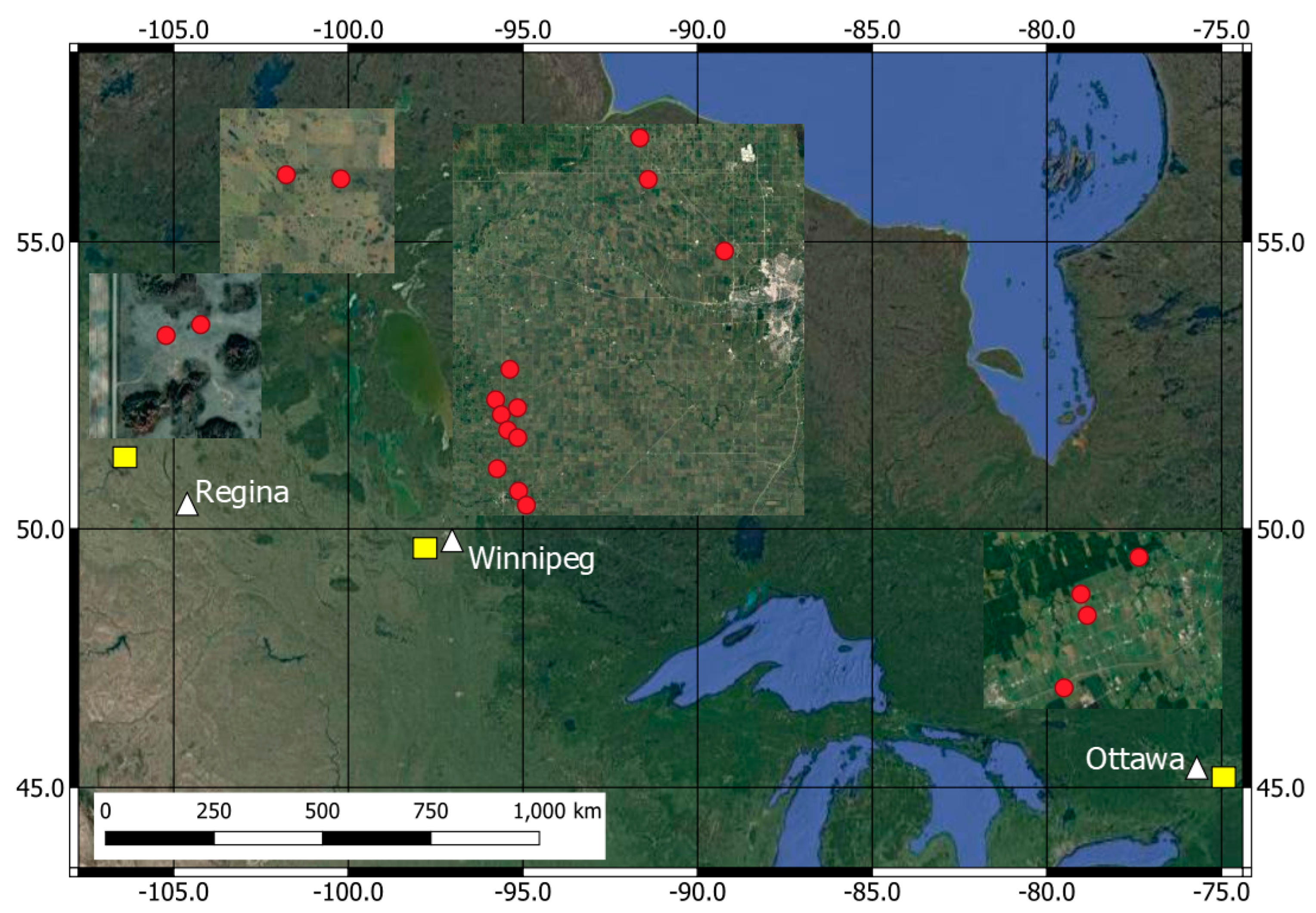
An experimental dataset collected over three Canadian test sites (Figure 1) was used for modeling the ML techniques in our study. The experimental dataset was constructed from a set of 127 RADARSAT Constellation Mission (RCM) images acquired by the SC30M Compact Polarimetric (SC30MCP) imaging mode over the three selected sites. This is a ScanSAR imaging mode of RCM with a spatial resolution of 30 m. All the acquired RCM images were multilooked (2 × 2) Ground Range Detected (GRD) products, providing the amplitude information of the backscattered signal. The speckle noise was further reduced by applying a 3 × 3 boxcar filter to the acquired images. All three sites are equipped with Real-Time In-situ Soil Monitoring for Agriculture (RISMA) stations. These stations include Stevens HydraProbe sensors that record the soil temperature and the real dielectric permittivity, which is converted to a volumetric soil moisture value [26].
The first site is located within the South Nation River watershed, close to the town of Casselman southeast of Ottawa, and has one RISMA network with four stations (Figure 1). The second site consists of two RISMA networks in southern Manitoba. The first network consists of nine RISMA stations located near the towns of Carman and Elm Creek, southwest of the city of Winnipeg. The second network consists of three stations immediately northwest of the city of Winnipeg, in the Sturgeon Creek watershed (Figure 1). The first and second test sites are characterized by intensive agriculture activities dominated by annual crops [27]. The third site is in Saskatchewan near the town of Kenaston, northwest of Regina. This site is characterized by pastures and has a network of four RISMA stations (Figure 1). The three selected test sites are characterized by flat earth surface without topographic features.
The RCM imagery (127 images) was acquired over the three test sites during the spring (April–June) of 2020 and 2021 and the fall (October) of 2021. The constructed sample dataset from three completely independent experimental sites with RCM imagery acquired in different seasons (spring and fall) and different years (2020 and 2021) ensured improved representativeness of the trained ML models. Furthermore, the selected time of the RCM imagery acquisition ensured no crops or significant row structures. Thus, fields were characterized by unvegetated bare soil with relatively smooth random roughness state. Subsequently, the radar signal reflectivity should be mainly triggered by the real dielectric constant of the soil. Furthermore, the weather information collected by the RISMA stations was used to confirm snow-free unfrozen soil conditions in spring and fall.
The experimental database consisted of 323 samples of radar backscattering coefficients, radar incidence angle, and soil moisture. Each sample corresponded to the mean backscattering in RH (right circular transmit and linear horizontal receive signal) and RV (right circular transmit and linear vertical receive signal), and the radar incidence angle (IA) at the location of a RISMA station, as well as the corresponding in situ soil moisture recorded at the time of image acquisition.
In our study, we considered the integrated soil moisture measured vertically from 0–5 cm due to the limited penetration capability of C-band SAR in bare soil [28]. However, during the early spring thaw, we instead considered the measured soil moisture at 5 cm. This is because the 0–5 cm sensor probes are inserted vertically at the soil surface, and in many instances the frost pushes the probes partially out of the ground during the spring thaw. This exposes the probe tines to the air and causes lower dielectric values, leading to underestimation of the integrated soil moisture measured vertically from 0–5 cm. Annually, Agriculture and Agri-Food Canada (AAFC) conducts the required maintenance of the stations before the middle of May by resetting the surface probes that have been displaced. The constructed experimental dataset of our study was characterized by a variety of soil moisture conditions, ranging from 5.8% (very dry conditions) to 46.4% (very wet conditions). However, most of the dataset samples had medium soil moisture values in the range of 15–25%. In our 323 samples, the minimum radar incidence angle was 20.8°, while the maximum was 42.9°. This is intentional following a recommendation by the RCM’s calibration and validation team, confirming the minor impact of the imperfect emitted RCM circular polarization signal, triggered by a dissimilarity between the H and V antenna gains, for a radar incidence angle between 20° and 43°. Within this range, the axis ratio of the transmitted signal was <0.5 dB.
3. Methodology
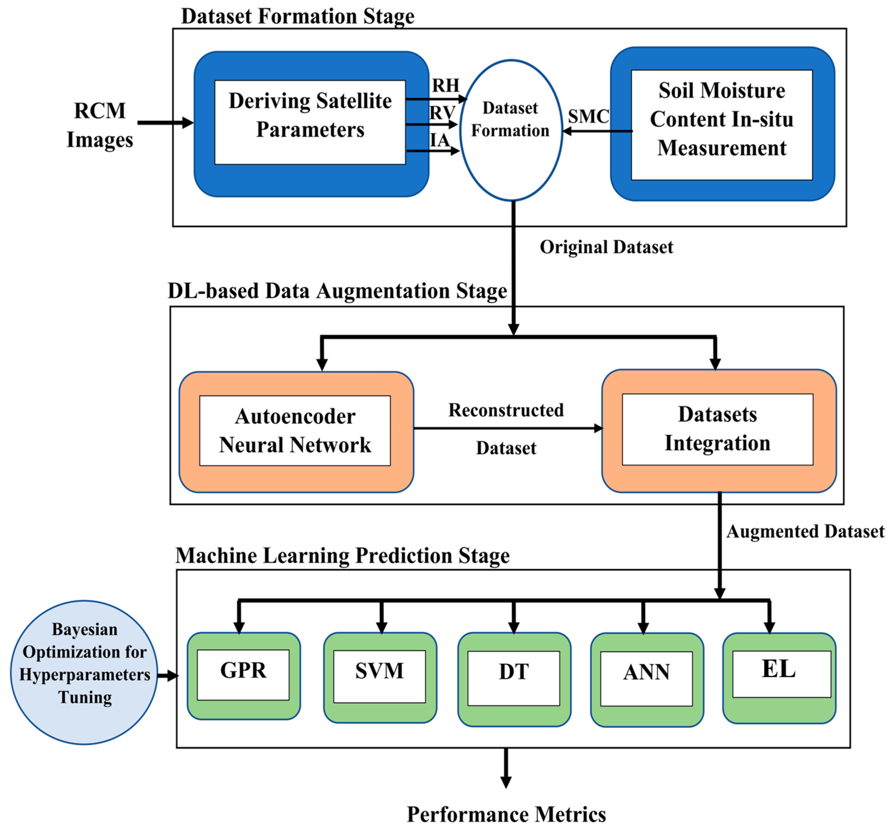
Due to the limited number of samples of the soil moisture dataset, oversampling was applied to boost the prediction performance of the ML regression models. In response to this demand, a DL-based framework was proposed to create an augmented dataset to promote the performance of several ML regression models in retrieving SMC. The proposed framework is presented in Figure 2. The introduced framework consists of three stages. In the first stage, the dataset was formed from the RCM SAR images as described in the previous section. In the second stage, a sparse autoencoder DL network was built to create a reconstructed version of the input features in the dataset samples. An augmented soil moisture dataset was then generated by integrating the original dataset with the autoencoder-based reconstructed dataset. The augmented soil moisture dataset was then used as input to several ML prediction techniques in the last stage of the framework for the purpose of soil moisture retrieval. The Bayesian optimization technique was utilized in this study to fine-tune the hyperparameters of the ML algorithms. The prediction performance of several ML regressors was measured and compared when trained using the augmented dataset and the original limited size dataset. The description of the ML techniques used in the current study is provided below.
3.1. ML Techniques Tuning
Tuning of the hyperparameters of the ML techniques is a critical process which has a significant impact on the ML prediction performance. Five of the popular ML techniques used in regression problems were considered in this study. Fine-tuning the hyperparameters of the ML regressors was conducted using the Bayesian optimization approach. The Bayesian optimization finds the hyperparameters’ values that minimize an objective or loss function [29]. The loss function that was utilized in this study is the mean squared error (MSE) between the predicted and the true target values. The Bayesian optimizer utilizes the expected improvement per second as the acquisition function [30], which selects the hyperparameter set of the upcoming iteration. The set of model hyperparameters that minimizes the upper confidence interval of the MSE objective function was considered the optimal set and the corresponding model was used for soil moisture prediction. In the following subsections, we present a brief description of the ML algorithms used in this study for the retrieval of soil moisture. The selection of the most suitable hyperparameters for tuning these ML models is presented as well.
3.1.1. Artificial Neural Network
ANN is a commonly used nonparametric ML technique for nonlinear classification and regression problems [31]. Each network consists of interconnected neurons and assigned weights which help in storing the acquired knowledge. In our study, the structure of the ANN is set by the Bayesian optimization. The Bayesian optimization was used to select the number of fully connected layers (excluding the final fully connected regression layer), the number of neurons in each layer, and the type of activation function. As the number of predictors is low and the data size is limited, the optimizer searched between one to three fully connected layers, and among integers log-scaled number of neurons between 1 to 300. The activation function could be rectified linear unit (ReLU), Tanh, Sigmoid, or no activation. The training regularization coefficient was also optimized over the log-scaled real values in the range [, ], where is the number of data samples.
Figure 3 shows the MSE optimization plot of the ANN which depicts the minimum observed and predicted MSE values versus the optimization iterations. The optimization algorithm ran for 30 iterations. The optimized ANN has three fully connected layers and a regression layer. The minimum MSE value recorded was 48.34 and the optimal hyperparameters that was selected by the Bayesian optimization at this MSE value were as follows: size of first layer = 60, size of second layer = 207, size of third layer = 18, activation function = ReLU, and regularization coefficient = .
3.1.2. Support Vector Machine
SVM is another commonly used nonparametric ML technique for nonlinear classification and regression problems. Herein, hyperplanes are defined for the optimum separation between classes with minimum error [31]. In this study, the SVM kernel function, kernel scale, epsilon, and box constraints were the hyperparameters tuned using the Bayesian optimization. The kernel function sets the type of the nonlinear transformation to be applied to the input data before training the model. The kernel scale controls the scale by which the kernel varies significantly with the input features. The box constraint determines the penalty enforced on data samples having large residuals. Epsilon is the reference value used to compare the prediction errors. In our study, the Bayesian optimization searched for the best set of hyperparameters that minimized the MSE function over 30 iterations. Table 1 shows the ranges of the SVM optimizable hyperparameters.
Figure 4 illustrates the MSE optimization plot of the SVM. The minimum MSE value recorded is 22.1 and the optimal hyperparameters were selected by the Bayesian optimization at this MSE value. The optimized SVM model had a Gaussian kernel with 0.0975 scale, the box constrain was 26.39, and epsilon was 2.0723.
3.1.3. Decision Trees
DT are nonparametric ML techniques which are based on the construction of an inverted decision tree to provide prediction in a classification or regression problem. In this study, regression trees (RT) were used for the soil moisture retrieval problem in hand. Each tree has a root node, internal nodes, and leaf nodes that partition the variable space using a set of hierarchical rules [22]. In our study, as we do not have missing values, no surrogate decision split was used. For the minimum leaf size hyperparameter, the Bayesian optimization searched the range [1 − where is the number of samples. The minimum leaf size determines the minimum number of samples that calculate the target variable of each leaf node [22]. Figure 5 presents the MSE optimization plot of the DT model. The lowest MSE value is 22.31 and the optimal hyperparameters have been selected by the Bayesian optimization at this MSE value. The optimized DT model has a Gaussian kernel with 0.0975 scale, a box constraint of 26.39, and epsilon of 2.0723.
3.1.4. Gaussian Process Regression
The GPR is a supervised nonparametric ML technique based on formation of time series prediction models using Gaussian processes [19]. There are several hyperparameters that need to be set for the GPR model. These hyperparameters include the basic function of the prior mean function of the GPR, the kernel function which models the correlation in the target variable, the kernel scale which sets the initial kernel parameters, and the samples noise standard deviation (σ). In our study, the Bayesian optimization technique selects the optimal hyperparameters from the ranges depicted in Table 2.
Figure 6 shows the optimization curve of the GPR model. Herein, the optimal hyperparameters are recorded at MSE value of 13.46 and are listed as:
- Basic function: Linear,
- Kernel function: Nonisotropic Rational Quadratic,
- σ: .
3.1.5. Ensemble Learning
EL is based on the concept of adopting multiple ML models for addressing nonlinear classification and regression problems, instead of a single model. An ensemble of decision tree-based models (weak learners) is generated and combined into a strong prediction model [3]. In our study, Boosted trees and Bagged trees were examined by the Bayesian optimization for the regression problem. The ensemble method in the Boosted trees was the least squares boosting (LSBoost) with RT learners. On the other, the Bootstrap bagging (Bag) with RT learners was the ensemble fashion of the Bagged trees. The minimum leaf size, learning rate, number of learners, and the number of predictors to sample were the optimizable hyperparameters of the ensemble models. Table 3 presents the ranges of these hyperparameters to be searched by the Bayesian optimization technique.
Figure 7 illustrates the minimum MSE plot over the optimization iterations for the ensemble model. The best point hyperparameter was obtained at a MSE value of 19.55. The optimal model is an LSBoost ensemble with 499 learners and a minimum leaf size of 2, learning rate of 0.10086, and a predictor to sample ratio of 1.
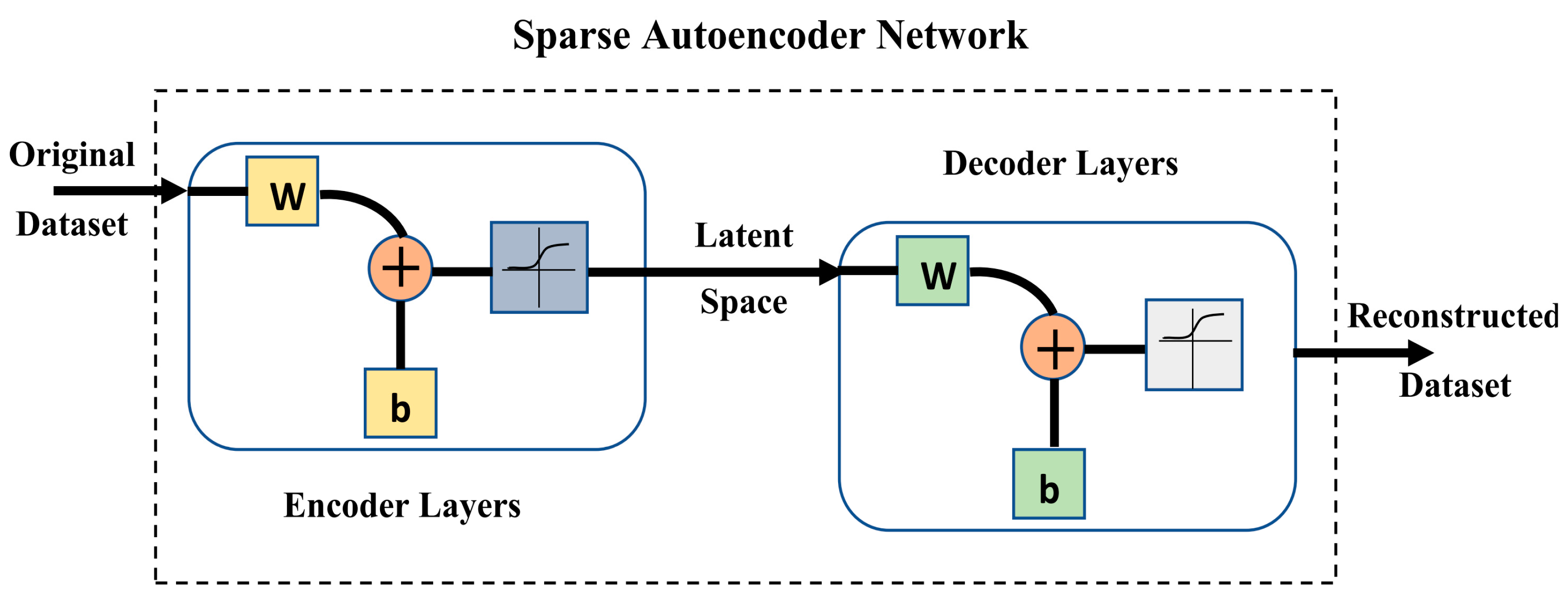
3.2. Autoencoder Deep Learning Neural Networks
Autoencoders are a special type of DL techniques that learn deep representation of the input data, map it into latent space, and then reconstruct the output from this representation in an unsupervised fashion [32]. Through symmetric encoder-decoder neural network architecture, autoencoder could reconstruct input data by applying backpropagation when the target is set to be equal to the input. The encoder compresses the input into a latent-space representation while the decoder reconstructs the input from this representation. The latent-space representational capability of autoencoder network enables it to learn effective features from the input data. This makes it of great use for dimensionality reduction, denoising, and reconstruction of input data [32,33]. Autoencoder, as any neural network, is built of input, output, and hidden layers. The number of nodes in the input and output layers is the same while the number of nodes in the hidden layers may be more or less than the input layer depending on the required task. In undercomplete and variational autoencoders, the hidden layer looks like a bottleneck with fewer numbers of nodes than those of the input layer. However, in overcomplete and sparse autoencoders, the opposite applies [32]. In our study, sparse autoencoder (SAE) is used to generate a constructed set of samples from the input dataset to build augmented soil moisture dataset to boost the prediction performance of ML-based soil moisture retrieval models.
Sparse autoencoders are a type of autoencoders in which the latent space layers contain a greater number of nodes than the input/output layers. On the hidden layers, sparsity constraints are imposed to select which node to be used for data representation according to its activation level [30]. This forces the network to learn a compressed representation of the data and use it in the reconstruction process. This prevents the output layer from copying input data and overfitting. Sparsity can be imposed by adding two regularization terms to the reconstruction error function,, during the training phase: L1 regularization and the Kullback–Leibler divergence () [34]. The reconstruction error measures the differences between the original input sample and the corresponding reconstructed input (). The L1 regularization term penalizes the absolute activations of the nodes of the hidden layers for an input data sample. This penalty on the sum of the nodes activations is determined by a custom coefficient λ. To define the , a sparsity parameter is defined to represent the average activation of a node in a hidden layer over a number of input samples. The constrained reconstruction error function, , is depicted in Equations (1) and (2) [34]
where is the input data sample, is the corresponding reconstructed sample of , and is the activation of a node in a hidden layer () for the input sample. The third term of Equation (2) presents the term. enables the comparison of the ideal distribution of to the observed distributions over all nodes in all hidden layers (). represents the operator and the coefficient determines the impact of the regularizer on the error function. The parameter , as given in Equation (3), represents the expectation activation of the node in a hidden layer () over a number of input samples ().
4. Results and Discussion
According to the proposed framework, the samples of the soil moisture dataset, composed from the SAR-derived parameters and their corresponding soil moisture values, were augmented using the sparse autoencoder. The number of autoencoder hidden representations was set to eight. The logistic sigmoid function was used as the encoder transfer function and the pure linear function was set as the decoder transfer function. The L1 regularization coefficient (λ) and the KLD coefficient () were set to 0.001 and 0.05, respectively. The SAE was unsupervised, which we trained using the scaled conjugate gradient algorithm over 2000 epochs. A stopping condition was applied if either the gradient or the error function reaches a predefined threshold value. The initial, end, and threshold values of the SAE gradient, as well as the constrained reconstruction error are depicted in Table 4.
The reconstruction performance of the SAE is given in Figure 9. This plot shows a reduction in the reconstruction error over the training epochs. The error curve attained the best stable error value of 0.028 starting from 1600 epochs and the training was stopped at 2000 epochs because the stopping condition was not attained.
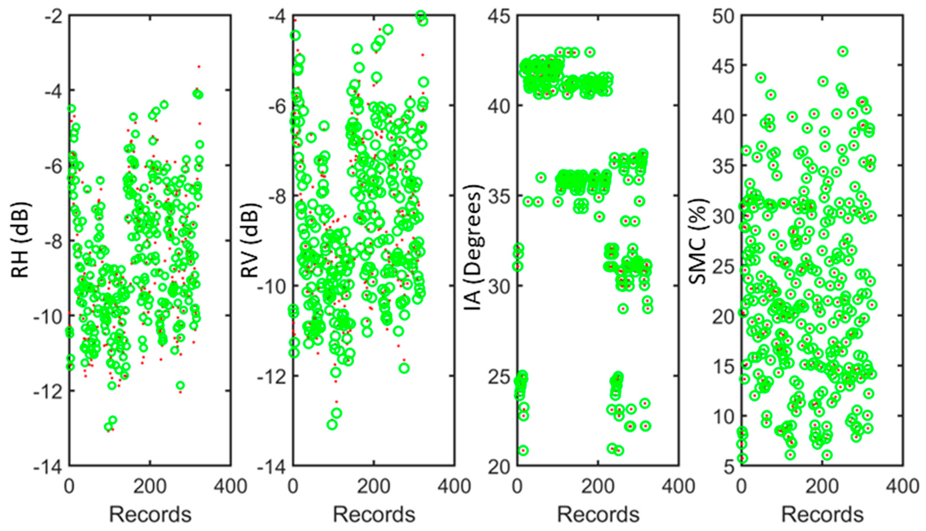
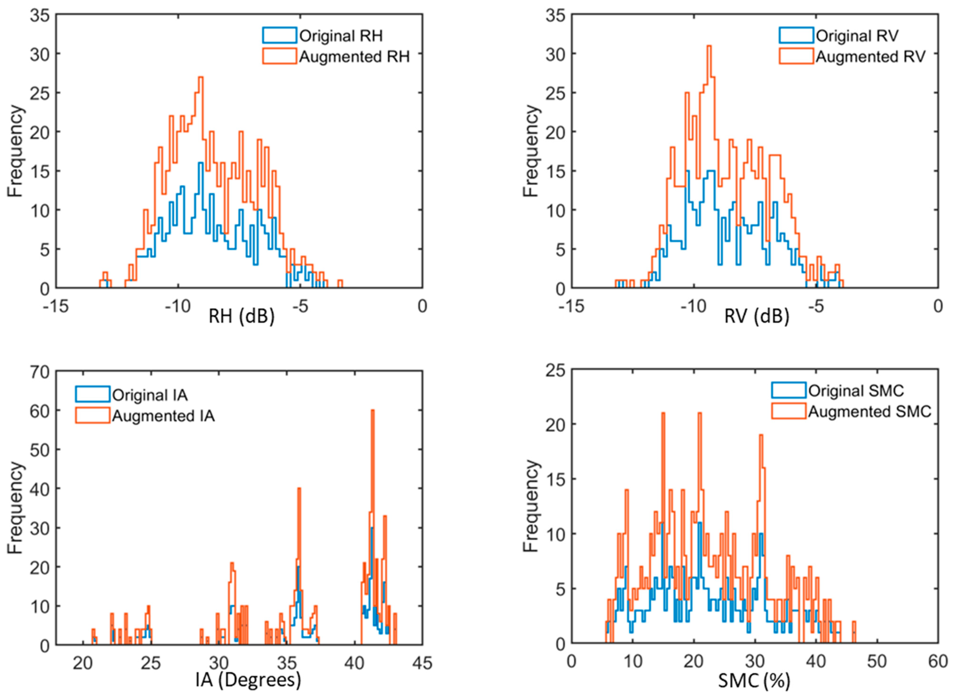
Figure 10 illustrates the augmented dataset which is composed of the original and reconstructed RH, RV, IA, and SMC. It is noticed that the reconstructed IA and SMC mostly coincide on the original values. However, deviation between the original values and the autoencoder-derived parameters is recorded for RV and RH. To further investigate the augmented dataset, histograms of the original and augmented variables are depicted in Figure 11. It has been noticed from Figure 11 that the histogram of the augmented RH differs from that of the original RH. This is also the case for RV. On the other hand, the histograms of the augmented IA and SMC reflect the high resemblance of the reconstructed and original variables. This observation enforces the aforementioned finding drawn from Figure 10. Moreover, it is obvious from Figure 11 that the histograms of the augmented variables cover the entire range of the original variables. Also, it is noticeable from the histograms that the distributions of the original and augmented variables are the same. This reconstruction behavior aids in providing an augmented dataset without duplicating the original samples which helps avoiding potential overfitting of the ML algorithms.
Five optimized ML regressors (DT, GPR, EL, SVM, and ANN) were used to predict the soil moisture in two experiments. These experiments were conducted to investigate the impact of the used DL-based sample augmentation on the retrieval performance of the five ML regressors. In the first experiment, the original non-augmented soil moisture dataset was used while in the second experiment, the SAE-based augmented dataset was utilized for the prediction of the soil moisture. The training was carried out using an eight-fold cross validation training scheme with a 10% holdout test set. The hyperparameters of the ML algorithms have been optimized using the Bayesian optimization. The RMSE and the coefficient of determination (R2), with R equal to the correlation coefficient, are used to measure the prediction performance of the algorithms.
- Experiment 1:
The results of this experiment are depicted in Table 5, which presents the prediction performance of the used ML regressors that have been trained on the original non-augmented dataset. It is observed that the RMSE is high for all the ML algorithms with low R2. This reflects the inadequate capability of the ML algorithms to model the structure of the input dataset, which should be triggered by the limited number of the dataset samples, though a cross validation scheme is used for training. The best validation and testing performance was recorded for the GPR model, with RMSE equal to 7.82% and 7.22% and R2 equal to 0.30 and 0.38, respectively. The entries of the best model (the GPR model) are highlighted in grey color in Table 5. The DT showed the highest RMSE and lowest R2 values in the validation compared to all other models, with RMSE equal to 9.31% and R2 equal to 0.01. In the testing, the lowest performance is observed for the SVM model, with RMSE equal to 8.49% and R2 equal to 0.14. We note that for all ML models the testing performance presents lower RMSE and higher R2 when compared to the validation performance. The goodness-of-fit of the utilized ML models is presented in Figure 12. Herein, both scatterplots of the predicted soil moisture (PSM) against the true soil moisture (TSM) values and the residuals for the testing set are shown.
Figure 12 shows that the regression models developed to predict the true soil moisture demonstrate different predictive powers. These prediction powers are generally weak, especially for the case of the DT model. Herein, the DT model presents insensitivity to the different values of the true soil moisture. From Figure 12, the developed regression models of GPR, EL, SVM, and ANN tend to overestimate extremely low soil moisture values and to underestimate extremely high soil moisture values. This tendency should be triggered by the reduced frequency of occurrence of extreme soil moisture conditions in the original sample dataset.
- Experiment 2:
In this experiment, the effect of using the autoencoder-based augmented dataset on the prediction performance of the ML models has been investigated. Table 6 shows the obtained RMSE and R2 values for the eight-fold cross validation scheme and the holdout testing set. It is noticeable that the prediction performance is improved substantially for all regressors for both the validation and testing scenarios. This reveals the impact of the SAE-based oversampling in improving the prediction performance of the developed regression models. The GPR model recorded the best prediction performance with RMSE equal to 3.67% and R2 equal to 0.85 in the cross validation, and RMSE equal to 4.05% and R2 equal to 0.81 in the testing. The entries of the best performing model are highlighted in grey color in Table 6. Unlike the first experiment, we note that in the second experiment the validation performance in terms of RMSE and R2 of the developed regression models is better than that of the testing performance. This is true for all the regression models, except for the case of ANN model. The ANN model shows the weakest prediction power in the cross validation with RMSE equal to 8.15% and R2 equal to 0.24, while the DT model shows the lowest prediction power in the testing with RMSE equal to 7.34% and R2 equal to 0.38.
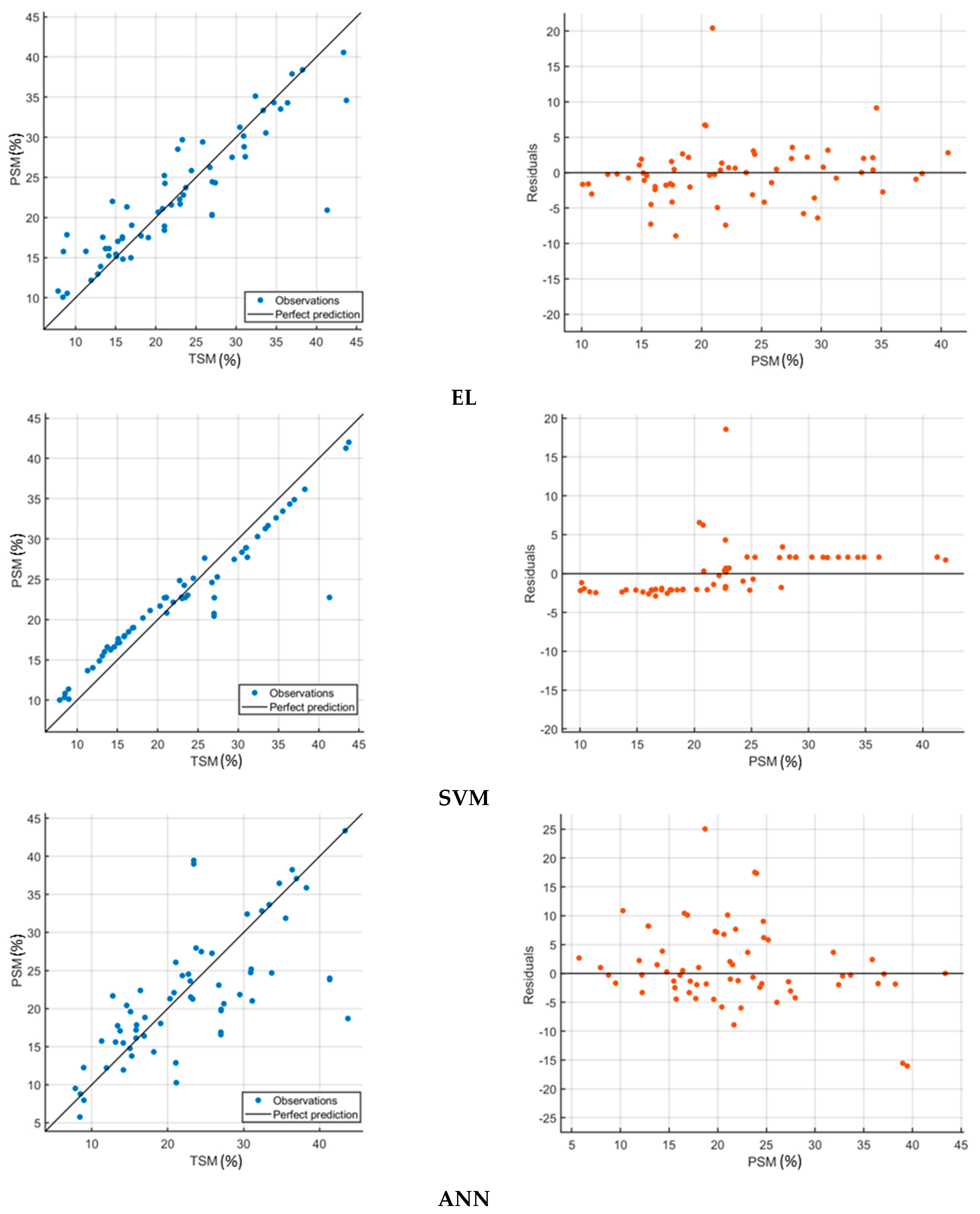
Figure 13 illustrates the goodness-of-fit of the regression models for the testing case. The PSM versus TSM scatterplots of the GPR model show the best fit on the augmented dataset over all the other models. This observation is confirmed by error values close to zero in the corresponding residual plot.
Figure 13 shows that the regression models developed to predict the true soil moisture demonstrate enhanced predictive power with the augmented sample dataset. We note that the sensitivity of the developed regression models to all possible soil moisture values is increased, which subsequently limits the overestimation or underestimation cases of these models at extreme soil moisture conditions.
5. Conclusions
In this study, a DL framework was proposed for the prediction of soil moisture content from satellite data using various optimized ML models. A dataset consisting of RH and RV radar backscattering coefficients and radar incidence angles sampled from acquired RCM images at the location of RISMA stations was used. A sparse autoencoder DL neural network was adopted to provide a reconstructed version of the input dataset. The original and the reconstructed dataset were integrated to form an augmented dataset with an increased number of samples for the purpose of promoting the prediction performance of the ML models. In this study, ANN, GPR, SVM, DT, and EL regression models were utilized for the retrieval of SMC. The hyperparameters of the ML regressors were tuned using the Bayesian optimization approach. The prediction performance in terms of the RMSE and goodness-of-fit was evaluated and compared for the ML algorithms trained on the original and augmented datasets. Findings of our study reveal the superiority of using the autoencoder network in enhancing the prediction performance of ML models. The obtained results showed that the GPR model consistently outperforms all the other ML models in retrieving the SMC. The GPR model recorded an RMSE value of 4.05% and R2 of 0.81 on an independent holdout test set, when using the augmented dataset for the ML training.
Author Contributions
M.D. and G.A. conceived the study. M.D. processed the SAR imagery. G.A. applied the DL framework. M.D., G.A., S.M. and W.A. analyzed the results. All authors contributed to the writing of the paper. All authors have read and agreed to the published version of the manuscript.
Funding
This work is supported by Princess Nourah bint Abdulrahman University Researchers Supporting Project number (PNURSP2023R196), Princess Nourah bint Abdulrahman University, Riyadh, Saudi Arabia.
Data Availability Statement
Not applicable.
Acknowledgments
The authors acknowledge the Princess Nourah bint Abdulrahman University Researchers Supporting Project number (PNURSP2023R196), Princess Nourah bint Abdulrahman University, Riyadh, Saudi Arabia. The authors would like to thank Agriculture and Agri-Food Canada (AAFC) for making the RISMA in situ soil moisture observations publicly available. Utilized sample dataset in this study was made available through a previous AAFC-Environment and Climate Change Canada collaboration project. RADARSAT Constellation Mission Imagery (c) Government of Canada (2023)-All Rights Reserved. RADARSAT is an official mark of the Canadian Space Agency.
Conflicts of Interest
The authors declare no conflict of interest.
References
- Lary, D.; Alavi, A.; Gandomi, A.; Walker, A. Machine learning in geosciences and remote sensing. Geosci. Front. 2015, 7, 3–10. [Google Scholar] [CrossRef] [Green Version]
- Sarker, I.H. Machine Learning: Algorithms, Real-World Applications and Research Directions. SN Comput. Sci. 2021, 2, 160. [Google Scholar] [CrossRef] [PubMed]
- Shirmard, H.; Farahbakhsh, E.; Müller, R.D.; Chandra, R. A review of machine learning in processing remote sensing data for mineral exploration. Remote Sens. Environ. 2022, 268, 112750. [Google Scholar] [CrossRef]
- Dawson, H.L.; Dubrule, O.; John, C.M. Impact of dataset size and convolutional neural network architecture on transfer learning for carbonate rock classification. Comput. Geosci. 2023, 171, 105284. [Google Scholar] [CrossRef]
- Shorten, C.; Khoshgoftaar, T.M. A survey on image data augmentation for deep learning. J. Big Data 2019, 6, 60. [Google Scholar] [CrossRef]
- Liu, L.; Davedu, S.; Fujisaki-Manome, A.; Hu, H.; Jablonowski, C.; Chu, P.Y. Machine learning model-based ice cover forecasting for a vital waterway in large lakes. J. Mar. Sci. Eng. 2022, 10, 1022. [Google Scholar] [CrossRef]
- De Kerf, T.; Gladines, J.; Sels, S.; Vanlanduit, S. Oil spill detection using machine learning and infrared images. Remote Sens. 2020, 12, 4090. [Google Scholar] [CrossRef]
- Wu, Y.; Duguay, C.; Xu, L. Assessment of machine learning classifiers for global lake ice cover mapping from MODIS TOA reflectance data. Remote Sens. Environ. 2020, 253, 112206. [Google Scholar] [CrossRef]
- López-Tapia, S.; Ruiz, P.; Smith, M.; Matthews, J.; Zercher, B.; Sydorenko, L.; Varia, N.; Jin, Y.; Wang, M.; Dunn, J.; et al. Machine learning with high-resolution aerial imagery and data fusion to improve and automate the detection of wetlands. Int. J. Appl. Earth Obs. Geoinf. 2021, 105, 102581. [Google Scholar] [CrossRef]
- Shahhosseini, M.; Hu, G.; Huber, I.; Archontoulis, S.V. Coupling machine learning and crop modeling improves crop yield prediction in the US Corn Belt. Sci. Rep. 2021, 11, 1606. [Google Scholar] [CrossRef]
- Santi, E.; Dabboor, M.; Pettinato, S.; Paloscia, S. Combining machine learning and compact polarimetry for estimating soil moisture from C-band SAR data. Remote Sens. 2019, 11, 2451. [Google Scholar] [CrossRef] [Green Version]
- Ghasemloo, N.; Matkan, A.; Alimohammadi, A.; Aghighi, H.; Mirbagheri, B. Estimating the agricultural farm soil moisture using spectral indices of Landsat 8, and Sentinel-1, and artificial neural networks. J. Geovis. Spat. Anal. 2022, 6, 19. [Google Scholar] [CrossRef]
- Kolassa, J.; Reichle, R.H.; Liu, Q.; Alemohammad, H.; Gentine, P.; Aida, K.; Asanuma, J.; Bircher, S.; Caldwell, T.; Colliander, A.; et al. Estimating surface soil moisture from SMAP observations using a neural network technique. Remote Sens. Environ. 2017, 204, 43–59. [Google Scholar] [CrossRef]
- Pekel, E. Estimation of soil moisture using decision tree regression. Theor. Appl. Climatol. 2020, 139, 1111–1119. [Google Scholar] [CrossRef]
- Kaur, A.; Neeru, N. Machine learning-based predictions for the estimation of soil moisture content. Comput. Integr. Manuf. Syst. 2022, 28, 265–281. [Google Scholar]
- Araya, S.N.; Fryjoff-Hung, A.; Anderson, A.; Viers, J.H.; Ghezzehei, T.A. Advances in soil moisture retrieval from multispectral remote sensing using unoccupied aircraft systems and machine learning techniques. Hydrol. Earth Syst. Sci. 2021, 25, 2739–2758. [Google Scholar] [CrossRef]
- He, B.; Jia, B.; Zhao, Y.; Wang, X.; Wei, M.; Dietzel, R. Estimate soil moisture of maize by combining support vector machine and chaotic whale optimization algorithm. Agric. Water Manag. 2022, 267, 107618. [Google Scholar] [CrossRef]
- Gill, M.; Asefa, T.; Kemblowski, M.; McKee, M. Soil moisture prediction using support vector machines. J. Am. Water Resour. Assoc. 2007, 42, 1033–1046. [Google Scholar] [CrossRef]
- Stamenkovic, J.; Guerriero, L.; Ferrazzoli, P.; Notarnicola, C.; Greifeneder, F.; Thiran, J.P. Soil moisture estimation by SAR in alpine fields using gaussian process regressor trained by model simulations. IEEE Trans. Geosci. Remote Sens. 2017, 55, 4899–4912. [Google Scholar] [CrossRef]
- Liu, M.; Huang, C.; Wang, L.; Zhang, Y.; Luo, X. Short-term soil moisture forecasting via gaussian process regression with sample selection. Water 2020, 12, 3085. [Google Scholar] [CrossRef]
- Taneja, P.; Vasava, H.B.; Fathololoumi, S.; Daggupati, P.; Biswas, A. Predicting soil organic matter and soil moisture content from digital camera images: Comparison of regression and machine learning approaches. Can. J. Soil Sci. 2022, 102, 767–784. [Google Scholar] [CrossRef]
- Carranza, C.; Nolet, C.; Pezij, M.; Ploeg, M. Root zone soil moisture estimation with Random Forest. J. Hydrol. 2020, 593, 125840. [Google Scholar] [CrossRef]
- Tramblay, Y.; Quintana Seguí, P. Estimating soil moisture conditions for drought monitoring with random forests and a simple soil moisture accounting scheme. Nat. Hazards Earth Syst. Sci. 2022, 22, 1325–1334. [Google Scholar] [CrossRef]
- Senyurek, V.; Farhad, M.M.; Gurbuz, A.C.; Kurum, M.; Adeli, A. Fusion of reflected GPS signals with multispectral imagery to estimate soil moisture at subfield scale from small UAS platforms. IEEE J. Sel. Top. Appl. Earth Obs. Remote Sens. 2022, 15, 6843–6855. [Google Scholar] [CrossRef]
- Dindaroğlu, T.; Kılıç, M.; Günal, E.; Gundogan, R.; Akay, A.; Seleiman, M. Multispectral UAV and satellite images for digital soil modeling with gradient descent boosting and artificial neural network. Earth Sci. Inform. 2022, 25, 2239–2263. [Google Scholar] [CrossRef]
- Pacheco, A.; L’Heureux, J.; McNairn, H.; Powers, J.; Howard, A.; Geng, X.; Rollin, P.; Gottfried, K.; Freeman, J.; Ojo, R.; et al. Real-Time In-Situ Soil Monitoring for Agriculture (RISMA) Network Metadata; Agriculture and Agri-Food Canada: Edmonton, AB, Canada. Available online: https://agriculture.canada.ca/SoilMonitoringStations/files/RISMA_Network_Metadata.pdf (accessed on 5 April 2022).
- McNairn, H.; Jackson, T.J.; Wiseman, G.; Belair, S.; Berg, A.; Bullock, A.; Colliander, A.; Cosh, M.H.; Kim, S.B.; Magagi, R.; et al. The soil moisture active passive validation experiment 2012 (SMAPVEX12): Prelaunch calibration and validation of the SMAP soil moisture algorithms. IEEE Trans. Geosci. Remote Sens. 2015, 53, 2784–2801. [Google Scholar] [CrossRef]
- Ulaby, F.T.; Moore, R.K.; Fung, A.K. Microwave Remote Sensing: Active and Passive; Artech House: Boston, MA, USA, 1986. [Google Scholar]
- Astudillo, R.; Frazier, P.I. Bayesian Optimization of Function Networks. In Proceedings of the 35th Conference on Neural Information Processing Systems, Online, 6–14 December 2021. [Google Scholar]
- Rasmussen, C.E.; Williams, C.K.I. Gaussian Processes for Machine Learning; The MIT Press: Cambridge, MA, USA, 2005. [Google Scholar]
- Senyurek, V.; Lei, F.; Boyd, D.; Kurum, M.; Gurbuz, A.C.; Moorhead, R. Machine learning-based CYGNSS soil moisture estimates over ISMN sites in CONUS. Remote Sens. 2020, 12, 1168. [Google Scholar] [CrossRef] [Green Version]
- Goodfellow, I.; Bengio, Y.; Courville, A. Deep Learning—Adaptive Computation and Machine Learning; The MIT Press: Cambridge, MA, USA, 2017; Volume 1. [Google Scholar]
- Atteia, G.; Collins, M.J.; Algarni, A.D.; Samee, N.A. Deep-Learning-Based Feature Extraction Approach for Significant Wave Height Prediction in SAR Mode Altimeter Data. Remote Sens. 2022, 14, 5569. [Google Scholar] [CrossRef]
- Olshausen, B.A.; Field, D.J. Sparse coding with an overcomplete basis set: A strategy employed by V1? Vis. Res. 1997, 37, 3311–3325. [Google Scholar] [CrossRef] [Green Version]
Figure 1.
Location of the experimental sites (yellow squares) with insets showing the RISMA stations (red circles).
Figure 1.
Location of the experimental sites (yellow squares) with insets showing the RISMA stations (red circles).

Figure 2.
The proposed DL-based framework for soil moisture retrieval.

Figure 3.
MSE optimization plot of the ANN model.

Figure 4.
MSE optimization plot of the SVM model.

Figure 5.
MSE optimization plot of the DT model.

Figure 6.
MSE optimization plot of the GPR model.

Figure 7.
MSE optimization plot of the EL model.

Figure 8.
Sparse autoencoder architecture. W and b represent the weight and bias of the neurons in the neural network layers, respectively.
Figure 8.
Sparse autoencoder architecture. W and b represent the weight and bias of the neurons in the neural network layers, respectively.

Figure 9.
The reconstruction performance of the SAE, which was utilized for sample dataset augmentation in this study.
Figure 9.
The reconstruction performance of the SAE, which was utilized for sample dataset augmentation in this study.

Figure 10.
Augmented soil moisture dataset parameters (RH, RV, IA, and SMC). Red dots present the original parameters; Green circles present the autoencoder-derived parameters.
Figure 10.
Augmented soil moisture dataset parameters (RH, RV, IA, and SMC). Red dots present the original parameters; Green circles present the autoencoder-derived parameters.

Figure 11.
Histogram plots of the original dataset parameters (RH, RV, IA, and SMC) versus the SAE-based augmented parameters.
Figure 11.
Histogram plots of the original dataset parameters (RH, RV, IA, and SMC) versus the SAE-based augmented parameters.

Figure 12.
Scatterplots of the prediction performance of the five optimized ML models trained on the original non-augmented dataset for soil moisture retrieval. Left: predicted versus true soil moisture; Right: residuals versus predicted soil moisture. Blue dots represent the observations, the diagonal line represents the perfect prediction, and the orange dots represent the residuals.


Figure 13.
Scatterplots of the prediction performance of the five optimized ML models trained on the SAE-based augmented soil moisture dataset. Left: predicted versus true SMC. Right: residuals versus predicted soil moisture. Blue dots represent the observations, the diagonal line represents the perfect prediction, and the orange dots represent the residuals.


Table 1.
The ranges of the SVM optimizable hyperparameters.
| Hyperparameter | Kernel Function | Kernel Scale | Box Constraint | Epsilon |
|---|---|---|---|---|
| Range | Linear Gaussian Cubic Quadratic | [0.001, 1000] | [0.001, 1000] | where is the target variable and is the Interquartile range of data. |
Table 2.
The ranges of the GPR optimizable hyperparameters.
| Hyperparameter | Basic Function | Kernel Function | Kernel Scale | σ |
|---|---|---|---|---|
| Range | Zero Constant Linear |
| Where, Where, is the predictor. | Where is the target variable. |
Table 3.
The ranges of the ensemble model optimizable hyperparameters.
| Hyperparameter | Ensemble Method | Minimum Leaf Size | Number of Learners | Learning Rate | Number of Predictors to Sample |
|---|---|---|---|---|---|
| Range | Bag/LSBoost | where, is the number of samples. | [10, 500] | [0.001, 1] | where is the number of predictors. |
Table 4.
The initial, end, and target values of the gradient and the constrained error function of the SAE.
Table 4.
The initial, end, and target values of the gradient and the constrained error function of the SAE.
| Initial Value | End Value | Threshold Value | |
|---|---|---|---|
| 426 | 0.028 | 0 | |
| Gradient | 21.9 | 0.011 |
Table 5.
Prediction performance of the five optimized ML models trained on the original non-augmented dataset for soil moisture retrieval. Performance metrics are measured over an 8-Fold cross validation scheme and for 10% holdout test set. The entries of the best performing model are highlighted in grey color.
| Optimized Model | 8-Fold Cross Validation | 10% Test Set | ||
|---|---|---|---|---|
| RMSE (%) | R2 | RMSE (%) | R2 | |
| DT | 9.31 | 0.01 | 7.90 | 0.26 |
| GPR | 7.82 | 0.30 | 7.22 | 0.38 |
| EL | 8.82 | 0.11 | 7.45 | 0.34 |
| SVM | 8.82 | 0.11 | 8.49 | 0.14 |
| ANN | 8.90 | 0.10 | 8.39 | 0.16 |
Table 6.
Prediction performance of the five optimized ML models trained on the SAE-based augmented dataset for soil moisture retrieval. Performance metrics are measured over an eight-fold cross validation scheme and for 10% holdout test set. The entries of the best performing model are highlighted in grey color.
| Optimized Model | 8-Fold Cross Validation | 10% Test Set | ||
|---|---|---|---|---|
| RMSE (%) | R2 | RMSE (%) | R2 | |
| DT | 6.83 | 0.46 | 7.34 | 0.38 |
| GPR | 3.67 | 0.85 | 4.05 | 0.81 |
| EL | 4.51 | 0.77 | 4.86 | 0.73 |
| SVM | 4.01 | 0.81 | 4.72 | 0.74 |
| ANN | 8.15 | 0.24 | 6.92 | 0.45 |
Disclaimer/Publisher’s Note: The statements, opinions and data contained in all publications are solely those of the individual author(s) and contributor(s) and not of MDPI and/or the editor(s). MDPI and/or the editor(s) disclaim responsibility for any injury to people or property resulting from any ideas, methods, instructions or products referred to in the content. |
© 2023 by the authors. Licensee MDPI, Basel, Switzerland. This article is an open access article distributed under the terms and conditions of the Creative Commons Attribution (CC BY) license (https://creativecommons.org/licenses/by/4.0/).
Share and Cite
MDPI and ACS Style
Dabboor, M.; Atteia, G.; Meshoul, S.; Alayed, W. Deep Learning-Based Framework for Soil Moisture Content Retrieval of Bare Soil from Satellite Data. Remote Sens. 2023, 15, 1916. https://doi.org/10.3390/rs15071916
AMA Style
Dabboor M, Atteia G, Meshoul S, Alayed W. Deep Learning-Based Framework for Soil Moisture Content Retrieval of Bare Soil from Satellite Data. Remote Sensing. 2023; 15(7):1916. https://doi.org/10.3390/rs15071916
Chicago/Turabian StyleDabboor, Mohammed, Ghada Atteia, Souham Meshoul, and Walaa Alayed. 2023. "Deep Learning-Based Framework for Soil Moisture Content Retrieval of Bare Soil from Satellite Data" Remote Sensing 15, no. 7: 1916. https://doi.org/10.3390/rs15071916
Note that from the first issue of 2016, this journal uses article numbers instead of page numbers. See further details here.