Article

Monitoring of Coastal Boulder Movements by Storms and Calculating Volumetric Parameters Using the Volume Differential Method Based on Point Cloud Difference

1
Department of Geography, University College London Gower Street, London WC1E 6BT, UK
2
School of Geography, Archaeology and Environmental Studies, University of the Witwatersrand, Johannesburg 2050, South Africa
3
Department of Civil, Environmental and Geomatic Engineering, University College London, Gower Street, London WC1E 6BT, UK
*
Author to whom correspondence should be addressed.
Remote Sens. 2023, 15(6), 1526; https://doi.org/10.3390/rs15061526
Submission received: 1 February 2023 / Revised: 7 March 2023 / Accepted: 8 March 2023 / Published: 10 March 2023
(This article belongs to the Special Issue Advances in Remote Sensing in Coastal Geomorphology Ⅱ)

Abstract

:
The measurements of boulder volume and axial length play significant roles in exploring the evolution of coastal boulder deposition, which provides a theoretical framework to examine the hydrodynamics of extreme wave events. At present, the application of structure-from-motion (SfM) to unmanned aerial system (UAS) imagery is one of the most used boulder surveying techniques. However, the monitoring of boulder movement and the accurate measurement of boulder morphometrics are rarely investigated in combination. In this study, UAS surveys were used to monitor moving boulders and measure boulder volumes using the volume differential method based on the differences of dense point clouds. This was undertaken at a site on the rocky shoreline of northwest Ireland in three repeated UAS surveys conducted in 2017, 2018, and 2019. The results from UAS monitoring and mapping of the distribution of 832 moving boulders in the study area over the 3-year period showed that boulders located in different zones of the coast vary significantly in their mobility. The main findings reveal that the theoretical error of the volume, obtained using the volume differential method, was estimated as 1–3.9%, which is much smaller than that of the conventional method of estimating volume using a tape measure.

Graphical Abstract

1. Introduction

In recent decades, various extreme sea wave events, triggered by storms and tsunamis, have caused significant damage and loss of life in many coastal areas around the world. For instance, Typhoon Haiyan, in the Philippines in 2013, resulted in an economic loss of up to 2 billion USD and at least 6300 deaths [1]. To more accurately reconstruct the intensity of the extreme wave events affecting a region, there has been extensive research into the movement and evolution of coastal boulders [2,3,4,5,6,7,8,9,10,11,12]. Since coastal boulders typically weigh several tons to tens of tons, they are resistant to average wave or tide conditions, and thus, changes in boulder distribution patterns across rocky shorelines can be considered a record of extreme coastal climate events [13,14,15]. Although several existing mathematical models have achieved the restoration of storm intensity and wave height [6,7,9,13,16,17,18,19], they remain heavily reliant on the accurate acquisition of certain parameters, such as the volume and axial length of boulders [20] in addition to regional wave climate buoy or wave model data.
The volume and axial length measurements of coastal boulders have been investigated in various regions around the world [3,4,5,6]. Before the emergence of new measurement techniques, the volume of a boulder was estimated by the length of a-, b- and c-axes (corresponding to the long, intermediate, and short axes of the boulder, respectively, measured with a tape measure in the field [4,6]), and it was assumed that the boulder was an idealised geometry. However, there is a large potential difference between the estimated volume and the real volume of a detached boulder. To solve this problem, Liu et al. [6] and Gennady et al. [4] used terrestrial laser scanner (TLS) and structure-from-motion (SfM) technologies on the ground to determine the real volume of the boulders more accurately. However, these two ground-based measurement technologies are restricted to measuring a single large boulder each time (low efficiency), and the cost of the TLS system is quite high. Therefore, studies have also applied unmanned aerial system- (UAS) SfM technology to collect datasets of study sites at a kilometre scale, using nadir or oblique photography and 3D photogrammetry software (Agisoft, Pix4DMapper), to perform modelling for volume calculations [3,5] or the monitoring of boulder movements [2]. Since multi-angle images can be captured using SfM technology based on oblique photography, the reconstruction of boulder size, shape, volume, and distribution is usually better than with SfM technology based on nadir photography. However, the cost of doing so means that the size of the survey area can be compromised. Although consideration is given to battery life and oblique photography, at the same time, when a 5-lens camera is used, the cost of UAS with 5-lenses is comparable to that of TLS technology. In addition, the above-mentioned techniques are not able to collect information from the bottom of a boulder, which adds to the uncertainty about volume calculations. The current approach is to simply close the bottom of the boulder model by using an artificial plain surface [4,5,6], but this can lead to more significant errors for the boulders on uneven surfaces.
At present, the calculation of boulder volume is not integrated with the monitoring of boulder movement from UAS surveys, and it is challenging in coastal environments comprising a large number of small boulders. This is because it is very difficult to detect the movement of small boulders (1–2 m in length) using even high-resolution satellite imagery. In this context, a method that combines the monitoring of boulder movement with accurate calculations of boulder volume is needed so that boulder movement and directions can be detected promptly and the volumes can be obtained with fewer UAS surveys. Further, the availability of different types of coastal boulder parameters facilitates the analysis of how extreme wave events caused by storms affect the movement of boulders.
The Multiscale Model-to-Model Cloud Comparison (M3C2) algorithm has been widely used to monitor environmental change, including coastal boulder movements [2], landslides [21], and riverbank erosion [22]. The M3C2 distance has a physical meaning, and in most cases, it can represent the thickness of a certain part of the boulder, which makes it possible to calculate the volume of the boulder. This study has built from this basis to calculate boulder volume using the M3C2 algorithm, and it has been applied to boulders mapped from repeated UAS surveys conducted along a rocky shoreline in northwest Ireland that has been previously examined for boulder dynamics [23,24]. The purpose of this application was to obtain boulder volumes and axial lengths in tandem with boulder movement over time and space from the UAS surveys. To support this analysis, a box group methodology (for simulating boulders) was used to verify the theoretical accuracy of this method.

2. Study Area

The study area is located on the Atlantic-facing northwest coast of Ireland at Falchorrib, County Donegal (Figure 1). This coastline has a northwest–southeast trend, and the rock shoreline examined in this study has a total length of about 1 km. Bedrock geology is rudaceous (coarse-grained) biotite granite that has developed distinctive sets of contraction joints that act as lines of weakness to weathering and erosion. The joint sets have acted as a first-order control in shore platform geometry, giving rise to a stepped profile in some places and deeply eroded, joint-aligned gullies in others. Hydraulic wave action contributes to the removal of individual bedrock boulders, as well as joint-defined slabs, from the shoreface; this provides the boulder supply for subsequent transport alongshore and into the upper intertidal zone, where distinctive boulder ridges are found [24]. Boulders are contained in the bedrock shore platform or within 20 m of it and are sourced entirely from the bedrock shoreline; the adjacent hinterland comprises a gentle slope covered almost entirely in peat bog. Northwest Ireland has a temperate maritime climate with onshore southwesterly winds, and this gives rise to its susceptibility to storms. The role of the storm wave forcing of boulder dynamics along the western Ireland coast has been examined in several studies [11,24,25,26].

3. Materials and Methods

The approach followed here involved four stages: (1) UAS surveys to collect nadir and oblique images of the boulders in the study area in 2017, 2018, and 2019, supported by dGPS surveying for ground control; (2) the application of Pix4DMapper 4.5.6 to generate high-density point clouds, orthomosaics, and digital surface models (DSMs) of the study area; (3) the application of CloudCompare to process the point clouds and calculate the M3C2 distance; (4) the use of Python and QGIS to calculate the M3C2 volume of the boulder and output the lengths of the a-, b-, and c-axes.
Practically, it is difficult to accurately measure the volume of boulders without moving them, and some are extremely large (several metres in diameter). To verify the feasibility and accuracy of the above method, multiple large shipping boxes with regular shapes were used to simulate boulders. The same approach outlined in stages 1–4 was followed to calculate the volume of the boxes and the length of the axes; these measurements were then compared with the actual dimensions of the boxes. This was used as an analogue to the boulders observed in the field in order to test the M3C2 method against boxes of known sizes.

3.1. Materials and Equipment

The initial data required for this study were divided into two parts: UAS images of the study area and ground control points (GCPs) obtained in the field. The UAS images were captured using the DJI Phantom 4 Pro drone, which is a relatively low-cost UAS that is applicable for the production of relatively high-quality image data. Having a built-in RGB camera with a 1” CMOS sensor, the Phantom 4 Pro is capable of capturing images with an effective pixel count of 20 MP. In addition, the camera has a nominal 8 mm focal length. It uses a global shutter instead of a rolling shutter, which is essential for the reconstruction of coastal boulders, as distortion can be caused by the rolling shutter. The built-in camera of the Phantom 4 Pro is also fitted with a stabilization system (gimbal) intended to prevent the shooting angle of the camera from being affected by drone movement. In flight, the camera system is in constant communication with the flight control system of the drone, which enables the camera to collect real-time data on the geographic position and attitude of the drone before writing it to each captured image file for later reconstruction.
The GCPs data were acquired using a Leica 1200 base station and a GS15 rover differential GPS system; surveyed ground control points and checkpoints were acquired with centimetre accuracy (average 3D coordinate quality of 0.014 m).

3.2. Acquisition of UAS Imagery and GCP Data

The ground sampling distance (GSD) was set to 2 cm, and the image overlap for each flight was set to at least 80% front overlap and 60% side overlap. High overlap has become a standardized operating procedure, ensuring that every point on the ground of the flight route is shown in a minimum of 5 images [27], and the benefits have been demonstrated in previous studies [28,29,30,31,32]. A single flight was used in the 2017 survey with a route direction aligned west–east to reduce cross-winds in light westerly winds. To obtain denser point clouds and more details from the reconstruction results, two flights were used in the 2018 and 2019 surveys, resulting in a total of 933 and 504 images, respectively.
Although each UAS image records the geographic coordinates and altitude at the time when the image is taken, the accuracy of the UAS GNSS receiver remains at the metre-scale, which is insufficient for the reconstruction of boulders on the spatial scale of less than 1 m. Therefore, it is necessary to process the reconstruction with accurate 3D GCPs. In total, this survey acquired 30 GCPs that are common to each survey by using natural discrete features across the bedrock platform, road, and jetty. The GCPs were surveyed into an Ordnance Survey of Ireland GPS benchmark located near the jerry at the northwestern end of the study area. Horizontal (x- and y-direction) and vertical (z-direction) coordinate quality (CQ) averages were 0.74 cm and 1.13 cm, respectively; these measures were used as the accuracy of GCPs in the Pix4DMapper.

3.3. Reconstruction of the Study Area Using Pix4DMapper

Separate projects were created for each year in Pix4D Mapper, and all UAS images for each year were imported. Pix4D uses the positioning, elevation, and shooting angle data contained in the image file for initial processing. Before adding GCPs, the full key point image scale is used, and the initial process (sparse reconstruction) is conducted. Once the sparse reconstruction is complete, a dense number of key points are generated across the study area—each of which can be found within multiple images. GCPs in the images for each year were marked manually and were first imported to identify a key point close to the GCP in the Pix4D software (Figure 2). Second, a new 3D control point was created, with the values of the 3D coordinates and the horizontal and vertical accuracy of this control point manually defined. With the position of the control point manually marked in at least two images, Pix4D can find all images where the control point is captured and mark them automatically. After the completion of automatic marking, each marked image is checked for fine adjustments, which ensures that they are close enough to the actual measurement point. If the control point features of an image are not captured clearly, the image is scaled down before marking, which results in the image carrying less weight in the subsequent reconstruction. Finally, the sparse reconstruction is re-optimized after all control points have been marked. Out of the 30 control points, 25 were used for sparse reconstruction, and 5 were selected to evaluate the accuracy of the final results.
The final constructed models include point clouds, DSMs, and orthomosaics. The following tests were conducted on multiple sets of parameter combinations:
  • For point cloud generation (dense reconstruction): The image scale in the point cloud densification was set to 1/2 and the multiscale was turned off to reduce noise. The point density was set to high, with each point requiring at least 2 matches, which can increase the detail and density of point cloud reconstruction.
  • DSM and orthomosaicing: Triangulation was used instead of inverse distance weighting, as it can improve clarity for the edges of the boulders. Since the resolution setting is consistent with the GSD (2 cm), each boulder can be better identified.

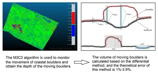
3.4. Calculation of M3C2 Distance

The Multiscale Model to Model Cloud Comparison (M3C2) algorithm was applied to calculate the distance distribution between two point clouds [21], which is a key step in determining change, boulder volume, and c-axis length. Typically, the two clouds should be aligned with each other before the M3C2 process, which causes a complete overlap of most areas (i.e., unchanged areas) of the point cloud model. The open-source software, CloudCompare, provides the tools used for point cloud alignment as well as access to the M3C2 plugin. The intuition provided by the tools and the plugin for monitoring the movement of coastal boulders has been tested and used in a previous study [2].
The core workflow using M3C2 is detailed as follows:
  • Importing the point cloud. Calculating the M3C2 distance requires two clouds, with one for reference and the other for comparison. In this project, the point cloud of the previous year was uniformly treated as the reference cloud; for example, the point cloud of 2017 was used as the reference cloud in the comparison between 2017 and 2018.
  • Setting the core point. The distance distribution between two point clouds was calculated based on several cell areas, which are usually divided from the original point cloud. The centres of these cell areas are core points, which are usually the reference point cloud itself or a subsample set. Here, the point cloud of the middle year (2018) was taken in this project as the core point to calculate the M3C2 distances of 2017–2018 and 2018–2019, thus reducing the systematic error of the volume calculations.
  • Defining normal vectors. Since the M3C2 algorithm calculates the distance between the reference cloud and the comparison cloud in terms of each core point, the normal vector of each core point is critical and defines the direction in which the distance from one cloud to another is calculated. Usually, a given value, D , is required to confirm the normal direction of the core point. Then, the M3C2 algorithm is applied to create a sphere with the core point as the sphere centre and D / 2 as the radius. The points contained within the sphere are fitted to a plane, and the normal vector of this plane is treated as the normal of this core point. However, any normal in a non-vertical direction was meaningless here (see Section 3.5 for an explanation), and the vertical direction was used directly.
  • Calculating the distance between two clouds. After the core point (i) and the normal vector (N) were determined, another parameter d was set for the M3C2 algorithm to make a circle with core point i as the centre and d / 2 as the radius. Subsequently, a cylinder was created along the axis of the normal vector that passed through the core point i. The parts of the two point clouds located inside the cylinder were defined as the n 1 and n 2 point cloud subsets. All the points in n 1 and n 2 were projected onto the cylindrical axis, with core point i as the origin, thus determining their distance distributions. The mean of these two distributions defined the average cloud positions, i 1 and i 2 , along the normal direction, while the distance between the two point clouds ( L M 3 C 2 ) was defined by the distance between i 1 and i 2 . In addition, it was necessary to input the maximum length of the cylinder to speed up the calculation process. In the cases of no corresponding point cloud data within the set length of the cylinder in the comparison cloud, the distance was not calculated.
  • Outputting M3C2 distance. The M3C2 distance value, as calculated based on each core point, was temporarily saved in a new point cloud composed of core points (the 2018 point cloud with RGB information removed herein). For the convenience of editing and reading, the results of this project were exported as a CSV file.

3.5. Calculation of the M3C2 Volume of Moving Boulders and Determination of the Length of the a-, b-, and c-Axes

The principle of differentiation was used to calculate the volume of the moving boulders, each of which was divided into several polygonal columns parallel to the z-axis of the coordinate system, as shown in Figure 3. The volume of the boulder was obtained by summing the volumes of all polygonal columns. It was expressed as:
d s · d h
where d s and d h represent the cross-sectional area and height of the polygonal column, respectively. This method involves the following steps:
  • Identifying moving boulders. In the M3C2 results, areas where values were significantly above or below 0 indicated boulder movement, keeping in mind that the surrounding bedrock does not change. QGIS was used to visualize the M3C2 results, with two orthomosaics, corresponding to the year, combined to identify the moving boulders.
  • Determining the edges of the boulder. Since accurate boulder edges are required for volume calculation, this study generated boulder edges manually to eliminate errors introduced by edge detection tools. The boulders whose volumes could not be calculated were excluded. Based on the visualization in step 1, the edges of the moving boulders were outlined using the orthomosaic of the study area and saved as a polygonal vector file.
  • Boulder outline gridding. This step was a process of differentials, using GIS tools to grid the boulder edges at set distances and calculate the area of each grid (which is the cross-section of the polygonal column, d s ). In this study, the grid was set to 2 cm, which was the GSD of the UAS surveys.
  • Determining the height of the polygonal column. Since the two point clouds had been finely aligned before the M3C2 algorithm was operated, the unchanged areas in the study area tended to be zero in the M3C2 results. Therefore, when a single boulder was moving, the M3C2 value (absolute value) of each core point in the area where the boulder was located could represent the height of that boulder in the vicinity of the core point (Figure 4). In the grid generated in step 3, there may have been one or more core points (M3C2 values) in some grids. In this situation, the maximum value of M3C2 was taken as the height ( d h ) of the polygonal column. In the case of no core point in the grid, the M3C2 value of the core point which was closest to the grid centre was treated as the height ( d h ) of the polygonal column. The advantage of using M3C2 core points to find the depth of boulders is reflected here. If two point clouds are directly used to calculate the elevation difference, the closest points found in the two point clouds may not be at the same position, which does not represent the depth of the boulder at a specific position very well. It is worth noting that the Z values of these core points are meaningless, as the grids only select core points in the horizontal direction and read the M3C2 value. This explains why only the vertical normal is selected in the M3C2 algorithm, as only the vertical d h is meaningful.
  • Calculating the boulder volume. The volume of each polygonal column was expressed as d s · d h (Equation (1)), and the sum of the volumes of all polygonal columns represents the theoretical volume of the boulder. According to the principle of differentiation, the smaller the grid scale and the higher the density of the core point, the closer the calculated theoretical volume is to the real volume.
It was relatively simple to obtain the length of the a-, b-, and c-axes of the boulder. The a- and b-axes could be directly measured using QGIS (Figure 5), while the c-axis was the maximum d h of all polygonal columns. In this section, the python code was used to go through steps 3–5 and output the length of the c-axis.

3.6. Accuracy Verification of M3C2 Volumes and Boulder Axis Lengths

In order to verify the feasibility and theoretical accuracy of the above method (Section 3.1, Section 3.2, Section 3.3, Section 3.4 and Section 3.5), the most straightforward solution is to compare the calculation results with the real values by referencing some boulders with known real volume and axes length. However, it is difficult to obtain the true volume and axes length of boulders in the field. As an alternative, large, regular-shaped shipping boxes were used to simulate coastal boulders. As shown in Figure 6, several boxes of the same specification were combined into three box groups. Group 1 and Group 3 each consisted of 6 boxes arranged in different ways, while Group 2 consisted of 2 boxes. The boxes in each group were strictly aligned without gaps and placed on flat ground. The length of the a-, b-, and c-axes of the box were 1.054 m, 0.248 m, and 0.742 m, respectively, as obtained through accurate measurement with a tape measure. The volume of each box group is expressed as:
V t = a · b · c · n
where a, b, and c represent the length of the a-axis, b-axis, and c-axis (m), respectively, of the original box; and n refers to the number of boxes in combination.
By using the same equipment, parameters, and analysis process followed for the coastal boulder analysis, UAS surveys were conducted on a planar site with (simulating the appearance of the boulder) and without (simulating the disappearance of a boulder) the boxes. The accuracy of the method employed was determined by comparing the calculation results with the measured dimensions.

4. Results

4.1. Results of Model Reconstruction

Figure 7 shows the 3-year point cloud models of the study area, as constructed by Pix4DMapper. The point clouds extended landward and seaward of the shore platform, so they were clipped to eliminate the vegetated hinterland, the sea, and areas not covered by all three surveys. The point clouds were clipped using a common boundary: after clipping, the number of points in 2017, 2018, and 2019 was 63,209,768, 107,638,302, and 138,540,087, respectively.
Orthomosaics and DSMs are generated using Pix4DMapper based on the point clouds, the accuracy of which can directly represent the accuracy of the cloud. Given the difficulty of visualizing the details of the boulder after the point cloud was enlarged and the computer power required for loading the point cloud, most of the follow-up work was based on orthomosaics, such as finding moving boulders, determining the boundaries of boulders, measuring the length of the a- and b-axes, and determining the horizontal accuracy of the point cloud. Although the DSMs were not used in the calculation of M3C2 volumes and boulder axis lengths, they could be loaded into QGIS along with the orthomosaics to determine the elevation accuracy of the point clouds.
The accuracy of the models in 2017, 2018, and 2019 was determined using five uniformly distributed GCPs (Figure 8, Table 1) not used in the Pix4DMapper reconstruction. The error near the northwest pier (id = 19, 46) was within 2 cm, which was clearly insignificant. In comparison, the error in the middle part (id = 52, 64) was relatively significant, reaching up to 36 cm. In addition, there were no GCPs in the southeastern corner of the study area. Through the misalignment of the orthomosaics, it could be found that the orthomosaic in 2019 had an overall horizontal misalignment in the southeastern corner, with an error of about 20 cm. This is because the southeastern corner of the study area in 2019 was located at the edge of the UAS survey area; there are fewer UAS images in this area, and the GCP correction is negligible.

4.2. M3C2 Results

The errors and misalignments, as described in Section 4.1, tend to have a substantial impact on the accuracy of M3C2 results, to which the only solution is to align the point clouds. According to the test results, the alignment of the full point cloud was ineffective because of the long and narrow extent of the survey area, with unevenness shown in the distribution of misalignment and error (Table 1). The scale of the unevenness was about 300 m (about 1.8 × 10 4   m 2 ), which was the largest theoretical scale for point cloud alignment in this study area. However, QGIS is more prone to collapse when loading point clouds (M3C2 results) at that size (approximately 200 million points), which is a necessary step to determine the edges of the moving boulder later. To deal with this issue, the area was divided into 18 sub-areas (the length range was 60–100 m, and the average area was 4800 m 2 , Figure 9), within which the alignment and M3C2 algorithms were run separately for each sub-area, thereby also significantly reducing the runtime. The alignment algorithm relies on fine registration (iterative closest point (ICP)). To improve the outcome of alignment, the root mean square (RMS) difference in the alignment algorithm was set to 10 6 m, the final overlap was set to 100%, and the random sampling limit was set to 100,000 points.
The cylinder diameter, d, was set to 0.1 m in the M3C2 algorithm, which is conducive to avoiding invalid M3C2 distances (i.e., no point in the comparison cloud can be found to calculate the distance). The maximum length of the cylinder was set to 5 m, and only the vertical normal vectors were used. After calculation, the core point with the added M3C2 result was maintained in its original 3D position and outputted as a temporary file. The visualisation of the resulting M3C2 distances (Figure 10) clearly highlighted unchanged regions, thus indicating successful alignment and boulder movement.

4.3. The Volume and Axial Lengths of the Boulder

The differential volume method based on the M3C2 distance is not suitable for volumetric calculations in all cases of moving boulders. If the moving distance is less than the scale of the boulder itself, the M3C2 algorithm cannot output all the elevation changes of the whole boulder unit. As shown in Figure 11, the M3C2 value of a part of this boulder (the blank area between red and blue) is close to 0, which makes it impossible to calculate the volume. Furthermore, if the area where the boulder contacts the surface changes, as shown in Figure 12, the M3C2 value is unfit to represent the thickness of the boulder. The stacking of boulders is common on this platform; again, this causes problems, as part of a stacked boulder can be suspended with a void between it and the underlying surface (Figure 13). Since the volume of the suspended part cannot be removed by the M3C2 distance, a considerable error arises.
Further issues arise when a boulder boundary is unrecognizable. Such cases include boulders with blurry borders, being shadowed, or being obscured by other boulders. Finally, orthomosaic misalignment (which occurs in the southeastern corner of the 2019 image) leads to issues in capturing the appropriate surface relative to the boulder. Boulder boundaries in sub-areas 16–18 in 2019 were not used for volume calculations. These three sub-areas can only be used to calculate the volume of the boulders whose boundaries were determined by the images from 2017 and 2018, and there is no way to calculate the volume of the boulders photographed in 2019. Finally, if it is determined that the same boulder appears twice in the M3C2 results (a boulder disappeared from one place in 2017 but appeared in another place in 2018, as shown in Figure 14), only the better one, such as the one with a clearer boundary, is used to calculate its volume. In this study, the same boulders corresponded with the same surface textures and edge shapes, which could identify sliding or flipping boulders. Most of the larger boulders in the study area are flattened, which helps them avoid complex rotational movements.
Comparing the change in shore platform point clouds between 2017 and 2018 (Figure 15a), 517 moving boulders, whose volume can be calculated, were identified in the study area. Among them, 202 boulders were located in the intertidal zone and 315 in the supratidal zone. According to the comparison between 2018 and 2019, the number of boulders whose volume could be calculated decreased to 378 (Figure 15b), of which, 256 boulders were in the intertidal and 122 in the supratidal zone.
All volume-computable boulders used the code mentioned in Section 3.5 to determine volume and c-axis length; then, the a- and b-axis lengths of the 20 largest boulders in both comparisons were measured in QGIS, and the estimated volumes of these boulders were calculated (Table 2). In conventional boulder volume estimates, the lengths of the a-, b-, and c-axes are used, with the boulders assumed to be idealised geometries, such as cuboids or ellipsoids. Some researchers use the correction factor V d G P S / V a b c to make the estimated volumes (product of a, b, and c) more accurate, where the V d G P S is the boulder volume, calculated using the coordinates of the boulder vertices and edges that were measured by dGPS [10,33,34]. According to previous studies [10,33,34], the value of the correction factor is in the range of 0.5–0.8, and the rather cubic boulders have higher correction factors. The standard ellipsoid volume was used to calculate the estimated volume in this study due to the large number of boulders. The volume of the ellipsoid is expressed as V = π a b c / 6 , which corresponded to a correction factor of π / 6 (0.524).
As revealed by the comparison between 2017 and 2018 (Table 2), 17 out of the 20 largest boulders were in the intertidal zone. The M3C2 volume of these boulders ranged between 0.38 m 3 and 1.85 m 3 , while the a-axis length varied between 1.12 m and 2.49 m. Comparatively, the conventional estimates of volume range from 0.28   m 3 to 1.61 m 3 . The estimated volumes are usually smaller than the M3C2 volumes, with their error between 0.43% and 26.75%. Of all the 517 boulders, 86.8% (449) had an M3C2 volume of less than 0.2 m 3 (Figure 16).
According to the comparison between 2018 and 2019 (Table 2), 18 out of the 20 largest boulders were in the intertidal zone. Their M3C2 volume and a-axis length were lower compared to the 2017–2018 period and were 0.22–0.95 m 3 and 0.90–1.87 m, respectively. The conventional estimate of volume ranges between 0.19 m 3 and 0.75   m 3 , and their error ranges from 0.03% to 41.19%. The M3C2 volume of all 378 boulders was less than 1 m 3 and was mostly below 0.2   m 3 (94.2%, 356 boulders, Figure 16).

4.4. Accuracy Verification Results

The volumes and axial lengths of the three test box groups were calculated using the same method as for the real boulders (Figure 17); the results of which are shown in Table 3. For the volume of M3C2, the error of the three box groups was around 0.01   m 3 , which was more favorable to the box group with a larger real volume. The error of the larger box groups (groups 1 and 3) was around 1%, while it was 3.9% for the smaller box group (group 2). For the a-axis and b-axis, the error of measurement result was about 1 cm (the error was less than 2%), while that of the c-axis ranged from 1.5 cm to 3 cm (the error percentage was up to 4.4%).

5. Discussion

5.1. Benefits of Differential Volume Calculation Based on M3C2 Distance

The theoretical accuracy that can be achieved using differential volume calculation based on the M3C2 distance has been demonstrated here. The error of the volume calculation result was only 1–3.9%, which is much smaller than the error of the boulder volume estimated using the conventional method of tape measuring (up to 36.9% [5]). In this study, there remained a significant error in the boulder volume estimated using the conventional method (up to 41.19%, Table 2) compared with the M3C2 volume, even though the accuracy of axial length calculation in this study has been improved compared to the manual tape measure [5,6]. The reduction of error in the M3C2 volume was attributed to the use of the real boundary of the boulder and the gridded boulder thickness statistics, which reduce the error caused by the conventional method of boulder volume estimation where the boulder is assumed to have an ideal geometry. In addition, the M3C2 distance was treated as the thickness of the boulder when the elevation change of the ground was taken into account, which solved the error caused by simplifying the bottom of the boulder to a plain surface. This is because other volume measurement methods are not applicable to obtaining the bottom information of the boulder. In addition to reducing volume errors, there are other advantages shown by the equipment and UAS survey parameters required for differential volume calculations based on M3C2 distances, such as low cost, high efficiency, and excellent safety performance. The cost of the UAS and dGPS systems are significantly lower than that of the TLS system, with higher measurement accuracy. Further, it is needless for researchers to perform dangerous measurement work on-site (such as climbing boulders, handling equipment, etc.). In terms of efficiency, with only nadir photography required, there will be more time saved for coastal boulder surveys in larger sites (e.g., a range of several kilometres) compared with oblique photography. In future work, UAS survey parameters can be adjusted according to actual needs to change the balance between accuracy and efficiency. For instance, given a confined research area, it is worthwhile to consider reducing GSD (e.g., 1 cm) or adding oblique images, which can help improve the accuracy of the 3D reconstruction model and volume calculation, despite the longer survey time.

5.2. Analysis of the Error between the M3C2 Volume and Real Volume of the Boulders

There remain errors between the M3C2 volumes and the real volumes of boulders, which to a large extent, result from the measurement of boulders that are not located on the rock platform surface but are suspended above it by resting on other boulders. Although all boulders were screened before the calculation of M3C2 volumes, and the evidently suspended boulders have been removed, it is unavoidable to have hidden suspensions that are not obvious from the orthomosaic. As indicated by the blue area in Figure 18, this inconspicuous suspension is caused by the shape of the boulder itself rather than other boulders. Located under the boulder, it can neither be displayed in the orthomosaic nor inferred from the surrounding objects. Since the image taken, based on the nadir photography, fails to provide sufficient detail required for the 3D reconstruction of the suspension, the actual outcome of the point cloud model reconstruction is marked by the red circles in Figure 18. The M3C2 value is ineffective at removing the height of the suspended part, which makes the M3C2 volume slightly larger than the real volume.

5.3. The Relationship between Coastal Boulder Movement and Storm Intensity

Previous studies and measurements [6,35] have shown that the initiating wave height of coastal boulders is proportional to the boulder size (axial length and volume). According to the results in Figure 16 and Table 2, the total number and maximum volume of boulders moved in 2017–2018 (517, 1.854 m 3 ) were significantly larger than those in 2018–2019 (378, 0.954 m 3 ). Storm intensity and wave height in 2017–2018 were greater than in 2018–2019, as confirmed by a review of storm observation data collected within the time frame of this study (Table 4). The reduction in the intensity of the storms in 2018–2019 resulted in lower boulder mobility, which allowed more boulders to remain in place without moving or moving out of the study area.

6. Conclusions

Through differential volume calculations based on M3C2 distances, the details of moving boulder bottoms were identified through comparisons, at least between different datasets obtained at different times, and the simplified treatment of boulder bottoms used in previous studies was optimized. By using accurate boulder boundaries and cm-scale gridded thickness statistics, this method improved the accuracy of boulder volume calculations (as low as 1.0–3.9%) compared to assuming the boulder has an ideal geometry. When only nadir photography was used, there was a considerable improvement in the endurance time of the UAS, making it possible to survey greater lengths of the coast. In addition, compared with the TLS system and the 5-lens oblique camera with higher precision, the differential method based on M3C2 distance can significantly reduce the cost of conducting a coastal survey while ensuring a relatively high level of accuracy, which is conducive to the development of higher-accuracy boulder (as well as ecological) surveys in the future.
In this study, volumes were calculated for 517 moving boulders along a rocky shoreline in northwest Ireland, for the 2017–2018 period. However, the number of moving boulders decreased to 378 in the 2018–2019 period.
In future research, the accuracy of boulder volume calculation can be further improved by reducing the GSD or adding oblique images. UAS surveys of coastal boulders could also be conducted before and after storms, and the model can be used to track the movement of single boulders in response to this forcing.

Author Contributions

Conceptualization, H.B. and D.G.; methodology, H.B. and Y.Y.; software, H.B. and Y.Y.; formal analysis, Y.Y.; investigation, Y.Y., H.B. and J.K.; data curation, H.B.; writing—original draft preparation, Y.Y.; writing—review and editing, H.B. and J.K.; supervision, H.B. and D.G. All authors have read and agreed to the published version of the manuscript.

Funding

This research received no external funding.

Data Availability Statement

Publicly available datasets were analysed in this study. These data can be found here: [https://1drv.ms/u/s!AkrDDM8CislFhWLPtnwcs7bwW7_E?e=1C0IUz] (accessed on 30 January 2023).

Conflicts of Interest

The authors declare no conflict of interest.

References

  1. Li, J.; Xue, J.; Wang, W.; Zhang, J.; Xu, Y. Analysis and enlightenment of the overseas important typhoon disaster in 2013. Meteorol. Disaster Reduct. Res. 2014, 37, 50–54. [Google Scholar]
  2. Nagle-McNaughton, T.; Cox, R. Measuring Change Using Quantitative Differencing of Repeat Structure-From-Motion Photogrammetry: The Effect of Storms on Coastal Boulder Deposits. Remote Sens. 2020, 12, 42. [Google Scholar] [CrossRef] [Green Version]
  3. Sedrati, M.; Morales, J.A.; El M’rini, A.; Anthony, E.J.; Bulot, G.; Le Gall, R.; Tadibaght, A. Using UAV and Structure-From-Motion Photogrammetry for the Detection of Boulder Movement by Storms on a Rocky Shore Platform in Laghdira, Northwest Morocco. Remote Sens. 2022, 14, 4102. [Google Scholar] [CrossRef]
  4. Gienko, G.A.; Terry, J.P. Three-dimensional modeling of coastal boulders using multi-view image measurements. Earth Surf. Process. Landf. 2014, 39, 853–864. [Google Scholar] [CrossRef]
  5. Boesl, F.; Engel, M.; Eco, R.C.; Galang, J.B.; Gonzalo, L.A.; Llanes, F.; Quix, E.; Brückner, H. Digital mapping of coastal boulders—High-resolution data acquisition to infer past and recent transport dynamics. Sedimentology 2020, 67, 1393–1410. [Google Scholar] [CrossRef]
  6. Liu, Z.; Zhou, L.; Gao, S. Application of the terrestrial laser scanner to the coastal boulders on the southern coast of Hainan Island. Haiyang Xuebao 2019, 41, 127–141. [Google Scholar]
  7. Terry, J.P.; Dunne, K.; Jankaew, K. Prehistorical frequency of high-energy marine inundation events driven by typhoons in the Bay of Bangkok (Thailand), interpreted from coastal carbonate boulders. Earth Surf. Process. Landf. 2016, 41, 553–562. [Google Scholar] [CrossRef]
  8. Kennedy, A.B.; Mori, N.; Yasuda, T.; Shimozono, T.; Tomiczek, T.; Donahue, A.; Shimura, T.; Imai, Y. Extreme block and boulder transport along a cliffed coastline (Calicoan Island, Philippines) during Super Typhoon Haiyan. Mar. Geol. 2017, 383, 65–77. [Google Scholar] [CrossRef] [Green Version]
  9. Goto, K.; Okada, K.; Imamura, F. Characteristics and hydrodynamics of boulders transported by storm waves at Kudaka Island, Japan. Mar. Geol. 2009, 262, 14–24. [Google Scholar] [CrossRef]
  10. May, S.M.; Engel, M.; Brill, D.; Cuadra, C.; Lagmay, A.M.F.; Santiago, J.; Suarez, J.K.; Reyes, M.; Brückner, H. Block and boulder transport in eastern Samar (Philippines) during Supertyphoon Haiyan. Earth Surf. Dyn. 2015, 3, 543–558. [Google Scholar] [CrossRef] [Green Version]
  11. Erdmann, W.; Kelletat, D.; Scheffers, A. Boulder transport by storms—Extreme-waves in the coastal zone of the Irish west coast. Mar. Geol. 2018, 399, 1–13. [Google Scholar] [CrossRef]
  12. Terry, J.P.; Jankaew, K.; Dunne, K. Coastal vulnerability to typhoon inundation in the Bay of Bangkok, Thailand? Evidence from carbonate boulder deposits on Ko Larn Island. Estuar. Coast. Shelf Sci. 2015, 165, 261–269. [Google Scholar] [CrossRef]
  13. Frohlich, C.; Hornbach, M.J.; Taylor, F.W.; Shen, C.-C.; Moala, A.; Morton, A.E.; Kruger, J. Huge erratic boulders in Tonga deposited by a prehistoric tsunami. Geology 2009, 37, 131–134. [Google Scholar] [CrossRef] [Green Version]
  14. Terry, J.P.; Lau, A.Y.A.; Etienne, S. Outlook for Boulder Studies within Tropical Geomorphology and Coastal Hazard Research; Springer: Berlin/Heidelberg, Germany, 2013; pp. 97–102. [Google Scholar]
  15. Terry, J.P.; Lau, A.Y.A.; Etienne, S. Reef-Platform Coral Boulders; Springer: Berlin/Heidelberg, Germany, 2013; pp. 97–102. [Google Scholar]
  16. Morton, R.A.; Gelfenbaum, G.; Jaffe, B.E. Physical criteria for distinguishing sandy tsunami and storm deposits using modern examples. Sediment. Geol. 2007, 200, 184–207. [Google Scholar] [CrossRef]
  17. Hall, A.M.; Hansom, J.D.; Williams, D.M.; Jarvis, J. Distribution, geomorphology and lithofacies of cliff-top storm deposits: Examples from the high-energy coasts of Scotland and Ireland. Mar. Geol. 2006, 232, 131–155. [Google Scholar] [CrossRef]
  18. Spiske, M.; Böröcz, Z.; Bahlburg, H. The role of porosity in discriminating between tsunami and hurricane emplacement of boulders—A case study from the Lesser Antilles, southern Caribbean. Earth Planet. Sci. Lett. 2008, 268, 384–396. [Google Scholar] [CrossRef]
  19. Etienne, S.; Paris, R. Boulder accumulations related to storms on the south coast of the Reykjanes Peninsula (Iceland). Geomorphology 2010, 114, 55–70. [Google Scholar] [CrossRef]
  20. Nandasena, N.A.K.; Paris, R.; Tanaka, N. Reassessment of hydrodynamic equations: Minimum flow velocity to initiate boulder transport by high energy events (storms, tsunamis). Mar. Geol. 2011, 281, 70–84. [Google Scholar] [CrossRef]
  21. Lague, D.; Brodu, N.; Leroux, J. Accurate 3D comparison of complex topography with terrestrial laser scanner: Application to the Rangitikei canyon (N-Z). ISPRS J. Photogramm. Remote Sens. 2013, 82, 10–26. [Google Scholar] [CrossRef] [Green Version]
  22. James, M.R.; Robson, S.; Smith, M.W. 3-D uncertainty-based topographic change detection with structure-from-motion photogrammetry: Precision maps for ground control and directly georeferenced surveys. Earth Surf. Process. Landf. 2017, 42, 1769–1788. [Google Scholar] [CrossRef]
  23. Knight, J.; Burningham, H.; Barrett-Mold, C. The geomorphology and controls on development of a boulder-strewn rock platform, NW Ireland. J. Coast. Res. 2009, 56, 1646–1650. [Google Scholar]
  24. Knight, J.; Burningham, H. Boulder dynamics on an Atlantic-facing coastline, northwest Ireland. Mar. Geol. 2011, 283, 56–65. [Google Scholar] [CrossRef]
  25. Scheffers, A.; Kelletat, D.; Haslett, S.; Scheffers, S.; Browne, T. Coastal boulder deposits in Galway Bay and the Aran Islands, western Ireland. Z. Geomorphol. 2010, 54, 247–279. [Google Scholar] [CrossRef]
  26. Cox, R.; Jahn, K.L.; Watkins, O.G.; Cox, P. Extraordinary boulder transport by storm waves (west of Ireland, winter 2013–2014), and criteria for analysing coastal boulder deposits. Earth Sci. Rev. 2018, 177, 623–636. [Google Scholar] [CrossRef]
  27. Furukawa, Y.; Curless, B.; Seitz, S. Towards internet-scale multi-view stereo. In Proceedings of the 2010 IEEE Conference on Computer Vision and Pattern Recognition, San Francisco, CA, USA, 13–18 June 2010; pp. 1434–1441. [Google Scholar]
  28. Grenzdörffer, G.J.; Engel, A.; Teichert, B. The photogrammetric potential of low-cost UAVs in forestry and agriculture. Int. Arch. Photogramm. Remote Sens. Spat. Inf. Sci. 2008, 31, 1207–1214. [Google Scholar]
  29. Mosbrucker, A.; Major, J.; Spicer, K.; Pitlick, J. Camera system considerations for geomorphic applications of SfM photogrammetry. Earth Surf. Process. Landf. 2017, 42, 969–986. [Google Scholar] [CrossRef] [Green Version]
  30. Henry, J.; Malet, J.; Maquaire, O.; Grussenmeyer, P. The use of small-format and low-altitude aerial photos for the realization of high resolution DEMs in mountainous areas: Application to the Super-Sauze earthflow (Alpes-de-Haute-Provence, France). Earth Surf. Process. Landf. 2002, 27, 1339–1350. [Google Scholar] [CrossRef] [Green Version]
  31. Torres-Sánchez, J.; López-Granados, F.; Borra-Serrano, I.; Peña, J. Assessing UAV-collected image overlap influence on computation time and digital surface model accuracy in olive orchards. Precis. Agric. 2017, 19, 115–133. [Google Scholar] [CrossRef]
  32. Mesas-Carrascosa, F.; Notario García, M.; Meroño de Larriva, J.; García-Ferrer, A. An Analysis of the Influence of Flight Parameters in the Generation of Unmanned Aerial Vehicle (UAV) Orthomosaicks to Survey Archaeological Areas. Sensors 2016, 16, 1838. [Google Scholar] [CrossRef] [Green Version]
  33. Engel, M.; May, S.M. Bonaire’s boulder fields revisited: Evidence for Holocene tsunami impact on the Leeward Antilles. Quat. Sci. Rev. 2012, 54, 126–141. [Google Scholar] [CrossRef]
  34. Hoffmeister, D.; Ntageretzis, K.; Aasen, H.; Curdt, C.; Hadler, H.; Willershäuser, T.; Bareth, G.; Brückner, H.; Vött, A. 3D model-based estimations of volume and mass of high-energy dislocated boulders in coastal areas of Greece by terrestrial laser scanning. Z. Geomorphol. 2014, 58, 115–135. [Google Scholar] [CrossRef]
  35. Nott, J. Waves, coastal boulder deposits and the importance of the pre-transport setting. Earth Planet. Sci. Lett. 2003, 210, 269–276. [Google Scholar] [CrossRef]
  36. UK Storm Season 2017/18. Available online: https://www.metoffice.gov.uk/weather/warnings-and-advice/uk-storm-centre/uk-storm-season-2017-18 (accessed on 24 April 2019).
  37. UK Storm Season 2018/19. Available online: https://www.metoffice.gov.uk/weather/warnings-and-advice/uk-storm-centre/uk-storm-season-2018-19 (accessed on 17 August 2020).
  38. Irish Weather Buoy Network Observations. Available online: http://www.marine.ie/site-area/data-services/real-time-observations/irish-weather-buoy-network-observations (accessed on 21 December 2022).
Figure 1. (a) The location of the study area in northwest Ireland, indicated by the red dot. (b) The study area is shown using satellite imagery. (c) A photo of the study area looking northwest. The surveyed area is located between the road and the sea and consists of a bedrock shore platform and boulders distributed on its surface.
Remotesensing 15 01526 g001
Figure 2. (a) A key point close to the GCP is chosen for manually marking the GCP on images. The orange arrow represents the selected key point, and the red arrow represents the measurement point of the GCP, which is the endpoint of a bedrock fracture (b).
Remotesensing 15 01526 g002
Figure 3. Illustration of the boulder gridding procedure.
Remotesensing 15 01526 g003
Figure 4. (a) M3C2 distance at different locations. Red and black circles represent the point clouds of the same region for two different years. The M3C2 values in the boulder-moving areas were significantly larger than those in unchanged areas. (b) The method used to determine the height ( d h ) of the polygon column. This is a side view of the M3C2 output, which is a point cloud comprised of core points (2018 point cloud with RGB information removed and M3C2 results added). The red, blue, and black circles indicate the core points where the M3C2 values were significantly above 0 (boulder appears), far below 0 (boulder disappears), and approaching 0 (no change), respectively.
Remotesensing 15 01526 g004
Figure 5. Measuring the length of the a-axis and b-axis in orthomosaics.
Remotesensing 15 01526 g005
Figure 6. Three box groups used to train the M3C2 model.
Remotesensing 15 01526 g006
Figure 7. Point cloud models for the three-year span, where the top row shows the original clouds outputted by Pix4DMapper, and the bottom row indicates the clipped clouds.
Remotesensing 15 01526 g007
Figure 8. Distribution of GCPs. The blue dots represent the 25 GCPs included in the Pix4DMapper calculations. The yellow dots represent the 5 GCPs used to confirm the accuracy achieved by the model, and the red range represents the research area.
Remotesensing 15 01526 g008
Figure 9. Sub-areas of the site used to improve point cloud alignment and computational efficiency.
Remotesensing 15 01526 g009
Figure 10. Visualization of M3C2 results in CloudCompare, where red (positive value) indicates the appearance of the boulder, blue (negative value) indicates the disappearance of the boulder, and green (value close to 0) indicates no change. To highlight boulder movements, the colour bar was adjusted to display the core points with M3C2 values between −0.15 m and 0.15 m in green, and the core points below −0.15 m and above 0.15 m in blue and red, respectively.
Remotesensing 15 01526 g010
Figure 11. Example of a boulder moving less than the scale itself. (a,b) show the location of the boulder in 2017 and 2018, respectively; (c) shows the M3C2 result of this boulder.
Remotesensing 15 01526 g011
Figure 12. An example of surface changes, where boulders in 2017 (a) moved away and new boulders moved in by 2018 (b), meaning that the surface beneath the boulders was not acquired in either survey.
Remotesensing 15 01526 g012
Figure 13. Partially suspended boulder, where (a,b) indicate the location of the boulder in 2017 and 2018 (disappeared), respectively.
Remotesensing 15 01526 g013
Figure 14. The movement path of a boulder. (a,b) indicate the location of the boulder in 2017 and 2018, respectively, while (c) shows the M3C2 results. The location in 2018 (red) was used to calculate the boulder volume.
Remotesensing 15 01526 g014
Figure 15. The distribution of volume-computable boulders, where (a) shows the comparison of 2017–2018, and (b) shows the comparison of 2018–2019. The red boundary represents the study area, the blue boundaries represent the boulders, and the yellow line represents the boundary between the intertidal and supratidal zones.
Remotesensing 15 01526 g015
Figure 16. Volume distribution of moving boulders in different time periods. More than half of the movable boulders were smaller than 0.1 m 3 , especially in the 2018–2019 period. The 2017–2018 period saw a greater number of larger boulders being moved.
Remotesensing 15 01526 g016
Figure 17. Accuracy was verified using box groups. (a) The orthomosaic and the boundaries of box groups 1 and 2. (b) The M3C2 results of box group 1, where the red dots indicate the values in excess of 0.15 m (box height), and the white dots indicate the values close to 0 (unchanged area).
Remotesensing 15 01526 g017
Figure 18. Errors caused by differential volume calculation based on M3C2 distance. The blue areas indicate the error area resulting from the suspension of the boulder. Red circles represent the point cloud model.
Remotesensing 15 01526 g018
Table 1. Error values for the 2017, 2018, and 2019 models at the positions of the 5 GCPs.
ID201720182019
Vertical Error (m)Horizontal Error (m)Vertical Error (m)Horizontal Error (m)Vertical Error (m)Horizontal Error (m)
190.0040.0260.0100.0260.0020.015
460.0390.0340.0060.0210.0100.048
520.3610.0610.1110.0770.3250.038
640.1930.0410.2860.0610.2090.083
730.0090.0450.0410.0680.0230.051
Table 2. The 20 largest boulders in the two comparisons, with the axial length, estimated volume ( V e ), M3C2 volume ( V M ), and error percentage ( e p ) calculated.
YearsSequencea-Axis (m)b-Axis (m)c-Axis (m) V e ( m 3 ) V M ( m 3 ) e p
2017–201812.4881.4760.8351.6051.854−13.4%
21.9521.4541.0081.4981.512−1.0%
31.3141.1780.8850.7170.935−23.3%
41.6240.9170.8540.6660.837−20.5%
51.8391.2450.6090.7300.6856.7%
61.5481.0770.8520.7440.64016.2%
71.6700.9250.5600.4530.594−23.8%
81.2041.1180.8720.6140.54911.9%
91.5980.8300.7130.4950.498−0.4%
101.5540.7860.6630.4240.474−10.5%
111.4050.8140.7760.4650.471−1.3%
121.3890.9620.7210.5040.4687.7%
131.3481.0130.48303450.429−19.5%
141.6441.2070.4760.4950.42716.0%
151.6420.7250.6190.3860.424−9.1%
161.1910.8520.7580.4030.418−3.7%
171.1191.1000.7960.5130.40526.8%
181.1510.8270.6370.3180.40421.4%
191.6141.0710.3140.2840.38526.3%
201.5591.0940.3650.3260.37813.9%
2018–201911.3111.1190.9820.7540.95421.0%
21.3051.0880.6630.4930.58215.3%
31.2690.8440.8580.4810.40917.6%
41.8690.8670.4900.4160.3906.6%
51.4100.8490.6240.3910.3637.7%
61.2190.8150.6430.3350.356−6.0%
71.3160.8920.5610.3450.3401.5%
81.4070.8880.6980.4570.32341.2%
91.2810.5480.6650.2440.309−21.0%
100.8950.8920.9040.3780.30324.8%
111.3490.8500.5700.3420.29217.2%
121.0800.7800.6020.2660.291−8.6%
131.2860.7730.4410.2300.286−19.7%
141.4290.7910.5030.2980.2787.2%
151.0600.7440.5650.2330.255−8.4
161.3290.6970.5130.2490.2490.0%
170.9580.8500.5900.2520.2481.4%
181.3020.8430.4830.2780.23816.7%
190.9720.6790.5520.1910.226−15.7%
201.2150.6450.5210.2140.219−2.2%
Table 3. Theoretical accuracy of the M3C2 method.
IDa-Axisb-Axis
Measured Value (m)True Value (m) e p Measured Value (m)True Value (m) e p
11.5041.4881.1%1.0571.0540.3%
21.0531.054−0.1%0.5060.4962.0%
31.0561.0540.2%0.7540.7421.6%
IDc-AxisVolume
Computed Value (m)True Value (m) e p Computed Value (m3)True Value (m3) e p
10.7750.7424.4%1.1511.164−1.1%
20.7730.7424.2%0.3730.388−3.9%
31.5021.4861.1%1.1761.1641.0%
Table 4. Storms affecting the northeast Atlantic between 18 September 2017 (survey in 2017) and 24 May 2019 (survey in 2019), with references to the maximum wave height and wind speed recorded in each [36,37,38].
YearsNameAppearance TimeMaximum Wind Speed (mph)Maximum Wave Height (m)
2017–2018Ophelia16–20 October 201711913.828
Brian19–23 October 20178515.938
Caroline6–11 December 20179311.25
Dylan30 December 2017–3 January 20187720.156
Eleanor2–5 January 201814020.156
Fionn14–21 January 201814720.625
David17–21 January 201812620.625
Georgina23–27 January 201814013.125
Emma26 February–7 March 2018142No Data
2018–2019Hector13–17 June 20187010.078
Helene16–21 September 2018789.375
Ali17–22 September 20181029.375
Bronagh20–25 September 2018968.438
Callum10–16 October 20187612.188
Diana27–30 November 201811015.703
Enk7–14 February 20198610.547
Gareth11–14 March 20198110.078
Hannah25–28 April 20198210.078
Disclaimer/Publisher’s Note: The statements, opinions and data contained in all publications are solely those of the individual author(s) and contributor(s) and not of MDPI and/or the editor(s). MDPI and/or the editor(s) disclaim responsibility for any injury to people or property resulting from any ideas, methods, instructions or products referred to in the content.

