Article

Calibration of Acoustic-Soil Discrete Element Model and Analysis of Influencing Factors on Accuracy

1
College of Engineering, China Agricultural University, Beijing 100083, China
2
Key Laboratory of Agricultural Equipment for Conservation Tillage, Ministry of Agricultural and Rural Affairs, Beijiing 100083, China
*
Author to whom correspondence should be addressed.
Remote Sens. 2023, 15(4), 943; https://doi.org/10.3390/rs15040943
Submission received: 29 December 2022 / Revised: 5 February 2023 / Accepted: 7 February 2023 / Published: 8 February 2023

Abstract

:
To obtain accurate soil parameters and improve the accuracy of the acoustic-soil discrete element simulation model, we studied the model’s parameter calibration. The simulation test was carried out using the measured acoustic velocity and dominant frequency as the response value (index). Firstly, the Plackett—Burman test scheme was used to obtain the sensitivity ranking of soil parameters to the dominant frequency and velocity of the acoustic wave. The parameters that significantly affect the acoustic wave were obtained: Shear modulus, Poisson’s ratio, and coefficient of restitution. Then the Box—Behnken test scheme was used to establish the regression relationship between the dominant frequency and the velocity of the sound wave and Shear modulus, Poisson’s ratio, and Coefficient of restitution. The results shows that the indexes that researchers focus on are different in different scenarios, and the sensitivity of soil parameters to different indicators is different, which results in different soil parameter values after calibration. This study analyzed the main factors affecting the accuracy of the acoustic-discrete element model in constructing the model, provided a method for improving the construction accuracy of the acoustic wave—soil discrete element model and provided a reference for the construction of discrete elements models in other fields.

Graphical Abstract

1. Introduction

There are more and more studies on the detection of farmland soil properties by acoustic waves, such as soil water content detection [1,2,3], soil compaction detection [4,5], and seed spatial position detection in soil [6], etc. To study the process of acoustic wave propagation in soil and clarify the propagation mechanism of the acoustic wave in discrete bodies to better guide practical applications, some scholars have introduced the discrete element method [7,8]. This method takes a single soil particle as an independent unit for calculation, can analyze information such as the force and motion of a single particle, and can visualize the acoustic wave propagation process. Therefore, it can promote the study of acoustic wave propagation in soil.
Parameter setting is a prerequisite for discrete element simulation, and the accuracy of the input parameters affects the error of simulation results, which is the key to whether the simulation can genuinely reflect the actual situation [9,10,11]. Parameter calibration can make soil particle simulation parameters conform to actual physical parameters, thus reflecting soil properties. Therefore, parameter calibration is critical in establishing an accurate acoustic-soil discrete element model. Due to the complexity of the soil structure, some constitutive parameters and contact parameters such as the shear modulus of soil particles, the rolling friction parameters between particles, and the restitution coefficient of collision between particles cannot be directly obtained in practical experiments [12,13]. At the same time, there is no detailed theory to establish the quantitative relationship between soil particle parameters and macroscopic mechanical response. Therefore, these parameters are currently obtained through parameter calibration methods [14,15,16,17,18,19]. That is, by continuously changing the soil particle parameters to obtain a set of simulation parameter combinations that can make the simulation experiment and the actual experiment macroscopic phenomenon consistent.
At present, there are two main methods for calibrating simulation parameters. One is the traditional calibration method with repose angle or sliding friction angle as a macro index. Nakashima analyzed the effect of gravity on different parameters (such as friction coefficient and rolling friction coefficient) by comparing the angle of repose of simulations and experiments to study the terrain-mechanical interaction under the condition of gravity on the lunar surface [20]. Marigo used the angle of repose as an index to calibrate cylindrical pellets [16]. The obtained parameters were used for the simulation of a rotating drum, and the simulation and experimental results were compared. While qualitative comparisons were good in most cases, there were some errors in quantitative comparison results. To get the soil particle parameters of the soil DEM (discrete element method) simulation model, Song Zhanhua calibrated the soil particle contact parameters with the soil repose angle and sliding friction angle as indexes [21]. The above calibrations are all calibrated by the traditional repose or sliding friction angle, and the same calibration indexes (angle of repose, interactive friction angle) are used for different application scenarios. Due to the significant differences in using scenarios, researchers pay attention to different indexes when establishing models, which may lead to that the models can not satisfy different scenarios and purposes. Therefore, it is necessary to search for the characteristic values that researchers pay special attention to in specific scenarios as calibration indexes according to the research purpose. The second is the method of calibration based on the actual scenario, calibrated by macro-indexes that can represent the main features of the material in the scenario. Coetzee determined the particles’ internal friction angle and stiffness values with a combination of shear and compression test results [17]. The calibration process is validated by modelling silo discharge and bucket filling. To develop a 3D numerical simulation model of burden distribution for the pre-reduction shaft furnace of COREX 3000, Li, Qiang determined the parameters of DEM (Discrete element method) by quantitatively comparing the angle of repose and discharge time of the hopper of simulation and experiment [19]. Furthermore, they verified the parameters’ feasibility. Shen Haohan calibrated the rock’s elastic modulus, Poisson’s ratio, and tensile strength, obtained various parameters of the particles, constructed a discrete element model of the rock, and verified the model by experiments [22]. In the above calibration experiments, according to different application scenarios, in addition to selecting the angle of repose index, other macro indexes that can represent the characteristics of the material and the critical indexes that researchers pay attention to during the experiment are also selected for calibration. This method can help researchers find the main particle parameters that affect macroscopic indexes, narrow the range of input parameters, and improve calibration accuracy. Therefore, the selected macro indexes for the calibration should be different for different application scenarios and research purposes.
In addition, when a single macro index is used for calibration, different particle parameter sets can be obtained; that is, one macro index can obtain many different particle parameter combinations. Each parameter combination satisfies the macroscopic phenomenon, so it is impossible to distinguish which parameter combinations are reliable. When the number of macroscopic indexes is increased to calibrate the particle parameters, the union of each parameter combination can be obtained to narrow the range of parameters to obtain a more accurate calibration effect. Therefore, the indexes that can characterize the material characteristics should be found according to the actual application scenario when calibrating. At the same time, the number of indexes should be increased as much as possible to improve the accuracy of parameter calibration.
According to the acoustic theory, the main characteristics of the wave are the velocity transmission and the dominant frequency, which are also two critical indexes in the acoustic analysis. Moreover, these two macroscopic indexes can be accurately measured in simulation and experiments. They are the macroscopic manifestation of the interaction between the soil medium and the acoustic wave, which can reflect the change of the acoustic wave in the medium to a certain extent. Therefore, in this research, the parameters of soil particles are fused and calibrated using the velocity and dominant frequency of the acoustic as indexes. In this research, the sandy soil is used as the calibration object, the acoustic velocity, and the dominant frequency of the received signal are used as the response, and the soil particle parameters that significantly affect the simulation results are screened through the Plackett—Burman test. Then, the significant parameters were calibrated by the Box—Behnken design test, and the optimal parameter combination was obtained, which was compared with the measured value to provide reliable soil particle parameters for building an accurate model of acoustic-soil interaction.
In addition, in the previous study, we have established a physical model of sound-soil propagation, so the introduction of the process of model establishment is relatively simple.

2. Materials and Methods

2.1. Actual Scene Experiment

To obtain the calibration indexes, a self-made acoustic wave test bench (Figure 1) [8] was used to get the value of acoustic velocity and dominant frequency. It includes the RGM-4005 universal material testing machine, ZBL-U5200 nonmetal ultrasonic tester, and self-made soil acoustic wave testing device. RGM-4005 Universal Material Tester is manufactured by Rigel Instruments Co., Ltd. and consists of a computer and a test machine host. The maximum load is 5 kN, and the relative error of the test force is within <1%. ZBL-U5200 non-metallic ultrasonic tester is manufactured by Beijing ZBL Science & Technology Co., Ltd. (Beijing, China). Ultrasonic time accuracy of this detector is ±0.025 μs, the sampling interval is 0.05 μs. The self-made soil acoustic wave testing device mainly included the box, excitation and receiving transducer, etc. The height, length, and thickness of the box were 130, 100 and 40 mm, respectively, which were the same as in the simulation.
The soil was dried by drying oven and the mass moisture content is 0%. After screening, soil particles with the particle size range of 1~2 mm were taken for the experiment. In this experiment the soil compression ratio was 12%. When starting the experiment, we filled the box with soil, and the size and shape of the box were the same as those of the discrete element model box. Then the universal material machine compressed the soil through the clamping block above the box until the compression ratio reached 12%, and the clamping block remained stationary. The acoustic experiment was carried out in a pressurized state. The transducer frequency was about 40 kHz. The excitation transducer excited the acoustic wave. The receiving transducer received the acoustic wave and collected the received signal waveform. Then, we calculated the wave velocity c and the dominant frequency F of the received signal. The measurement result was that the acoustic velocity was 507 m/s, and the dominant frequency was 18 kHz. The results were used as the target value (index) for discrete element calibration.

2.2. Simulation Model Establishment

2.2.1. DEM Calculation Method

An ideal model is used to reduce the influence of complex soil environments, such as different soil particle sizes and water content, on acoustic wave attenuation. The Hertz—Mindlin (no slip) model [23,24] was chosen for this study, which is mainly used for discrete-body simulations. Normal damping, tangential damping, normal stress, tangential stress, and friction forces and moment among soil particles are calculated as follows.
Normal force Fn:
F n = 4 3 E R δ n 3 2
1 E = ( 1 v i 2 ) E i + ( 1 v j 2 ) E j
1 R = 1 R i + 1 R j
where R* represents the equivalent radius; δn represents the normal overlap; E* represents the Young’s modulus, Rj and Ri represent the radius of the soil particles in contact; vj and vi represent the Poisson’s ratios of the soil particles in contact; Ej and Ei represent the Young’s modulus of the soil particles in contact.
Normal damping force F n d :
F n d = 2 5 6 β S n m v n r e l
β = ln e ln 2 e + π 2
S n = 2 E R δ n
m * = ( m i m j m i + m j ) 1
where Sn represents the normal stiffness; m* represents the equivalent mass; v n r e l represents the normal component of the relative velocity; β represents the damping coefficient.
The tangential force Ft depends on the tangential stiffness St and the tangential overlap δt.
F t = S t δ t
S t = 8 G R δ n
where v t r e l represents the relative velocity; G* represents the equivalent tangential modulus.
F t d = 2 5 6 β S t m v t r e l
τ i = μ r F n R i ω i
where Ri represents the distance of the contact point from the center of mass, ωi represents the unit angular velocity vector of the object at the contact point and μr represents the coefficient of rolling friction.

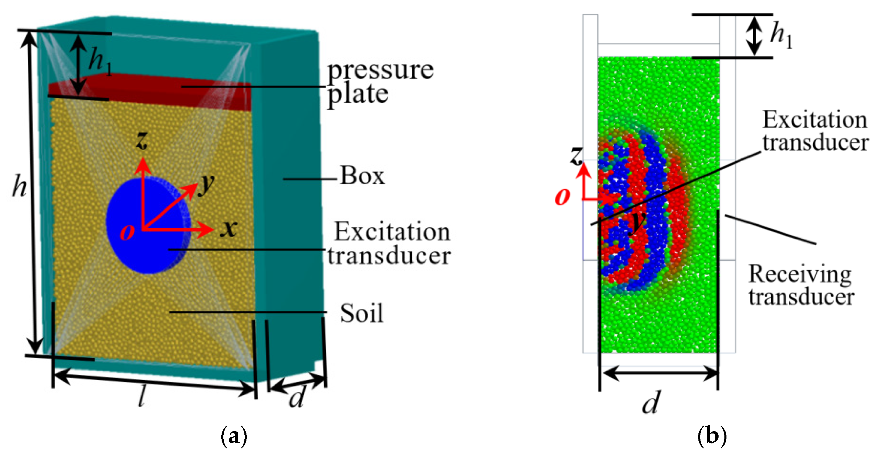
2.2.2. Discrete Element Model Building

Since this model has been established in previous research [8,25], the critical parameters and settings are briefly introduced. The DEM model is established according to the experimental bench, which only retains the soil, box, pressure plate, excitation transducer and receiving transducer related to acoustic wave propagation so as to obtain the propagation law of acoustic waves in soil. As shown in Figure 2a,b, the box is the same as the experiment. The soil is compressed by the pressure plate and the h1 is the downward distance of the pressure plate. The excitation transducer transmits acoustic signals, and the receiving transducer receives acoustic signals.

2.2.3. Simulation Parameter Settings

The particle size is 2 mm. The fixed time step is 1.0 × 10⁻⁸ s, 0.812% of the contact time. The grid cell sizes is 2 mm and the gravity is 9.8 m/s2. The number of soils is 600,000. The pressing plate compressed the soil until the compression ratio reached 12% (Equation (12)). The excitation transducer sends a single period sine wave to the soil in the y-axis direction (Figure 2b) [26]. The excitation amplitude A1 is set to 10 μm [27], and the excitation frequency f is 40 kHz, the same as the experiment. The relationship between the excitation transducer amplitude, frequency, phase angle, and period in the DEM model is shown in Equations (13)–(15).
α = h 1 / h
where h1 represents the soil compression height, mm; α represents the soil compression ratio; h represents the height of soil, mm.
y = A 1 sin θ
θ = 2 π f t
T = 1 / f
where A1 represents the maximum amplitude (displacement) of the transducer motion, um; y represents the instantaneous displacement, um; t represents the time, s; f represents the vibration frequency, Hz; T represents the motion period, s; θ represents the angle of phase, rad.
The aim of this research is to calibrate the parameters in soil particles that significantly affect the acoustic wave characteristics. The function of the transducer is to apply an external excitation to the soil, thereby sending out acoustic wave signals. The parameters of the transducer and the contact parameters between the transducer and the soil particles will not affect the propagation law of the acoustic wave in the soil. Furthermore, the box plays the role of containing the soil and does not affect the acoustic wave propagation process. For the above reasons, the parameters of the box and transducer and the contact parameters between them and soil particles are not focused. Determining parameter values mainly refers to previous literature [27,28,29]. The soil particle parameters were determined by calibration as factors of the experiment and will be described in detail in Section 3. The material of the pressure plate and the box is steel, and the transducer’s material is piezoelectric ceramics (pzt). Physical parameters and contact parameters are listed in Table 1 and Table 2, respectively.

2.3. Index Measurement

(1)
Acoustic velocity
The acoustic velocity is one of the main characteristics of the acoustic wave time—domain signal, which can reflect the physical properties of the transmission medium so that the acoustic velocity can be used to calibrate parameters. Figure 3a is the time—domain curve of the acoustic pressure P of the receiving transducer in the discrete element model.
c = d / Δ t
where d represents the transmission distance, in m; Δt represents the transmission time, in s.
(2)
Dominant frequency
The dominant frequency of an acoustic wave can reflect a large number of physical and mechanical properties of the medium. Therefore, the dominant frequency is taken as the calibration index. Figure 3 is the Fourier transform of the first wave of the received signal, and the calculation method is based on formula (17). The dominant frequency value F is the frequency corresponding to the maximum amplitude in the spectrum curve, as shown in Figure 3b. Similarly, the experimental calculation method is the same.
X [ k ] = n = 0 N 1 x n e i 2 π k n / n

2.4. Test Scheme

The constitutive parameters of soil particles reflect soil’s inherent properties, including particle shear modulus, Poisson’s ratio, and density. Since acoustic waves propagate in elastic media, the constitutive parameters of soil particles are essential parameters that affect the propagation characteristics. The contact parameters include the coefficient of restitution, the coefficient of static friction and the coefficient of kinetic friction of the particles. The contact parameters are related to the surface smoothness of the particles and the particles shape. In order to simplify the model, This paper replaces the soil particle shape with a spherical shape, so the contact parameters must be calibrated. Therefore, the experimental factors selected in this paper are particle density, Poisson’s ratio, shear modulus, coefficient of restitution, coefficient of static friction and coefficient of kinetic friction. Not all factors significantly affect acoustic wave propagation, so this paper uses the Plackett—Burman design screening test to analyze the sensitivity of the constitutive particle parameters and contact parameters and obtains the factors that significantly affect the soil acoustic wave propagation test. Subsequently, in order to obtain the best combination of soil parameters, the Box—Behnken test was carried out.

2.4.1. Plackett—Burman Test Scheme

The simulation test was carried out with the Poisson’s ratio, shear modulus, density, restitution coefficient, static friction coefficient and rolling friction coefficient of soil particles as the factors, and the acoustic velocity v and the dominant frequency F as the indexes. There are a total of 6 factors, each with a high and a low level. According to the literature [30,31,32], the range of the parameters value of soil particles is roughly obtained. The factors and levels are listed in Table 3.
Six factors, X1~X6, were selected for the Plackett—Burman experimental design with 12 experiments.

2.4.2. Box—Behnken Test Scheme

According to the results of the Plackett—Burman test, it can be seen that X3, X5 and X6 are insignificant factors, so we take the median value of soil parameters, which are 2650 kg/m3, 0.5, and 0.25, respectively. The Box—Behnken design test was applied to the significant factors to conduct response surface analysis and find the optimal solution. X1 (Poisson’s ratio), X2 (Shear modulus) and X4 (Coefficient of restitution) were used as test factors. The values of specific factors are shown in Table 4. The velocity and dominant frequency of acoustic waves are the test indexes.

3. Results and Discussion

3.1. Plackett—Burman Test Results and Sensitivity Analysis

Table 5 shows the simulation test results of acoustic velocity and dominant frequency under each factor level and analyzed by Design—Expert 8.0.6 software according to the results.
Table 6 shows the analysis of the variance of the Plackett—Burman experiment. It can be seen from the p-value that within the selected parameter value range, Poisson’s ratio (X1), Shear modulus (X2), and Coefficient of restitution (X4) have a significant impact on the acoustic velocity and dominant frequency.
Table 7 is the order of the contribution of each factor to the two indexes of the acoustic velocity and the dominant frequency of the received signal. It can be seen from the table that the order of the contribution of each factor to the acoustic velocity from large to small is X2 > X1 > X4 > X5 > X6 > X3; the order of influence on the dominant frequency of the acoustic wave is X2 > X1 > X4 > X6 > X3 > X5. In order to make the model optimization simple and feasible, Poisson’s ratio (X1), Shear modulus (X2), and Coefficient of restitution (X4), which have a significant impact on both indexes, are used for parameter calibration.

3.2. Box—Behnken Design Test

3.2.1. Establishment of Regression Model and Significance Analysis

In order to obtain the optimal combination of soil parameters, the Box—Behnken test was carried out, and the program and results are shown in Table 8. Quadratic regression fitting was performed on the experimental data in Table 8 by Design-Expert 8.0.6 software. The regression equation with the dominant frequency Y1 and the acoustic velocity Y2 as the response values and Poisson’s ratio (X1), Shear modulus (X2), and Coefficient of restitution (X4) as the variables are obtained.
(1)
Significance analysis of acoustic wave dominant frequency Y1
Table 9 shows that the regression model of the dominant frequency Y1 is p < 0.0001 (highly significant), and the lack of fit term is p = 0.7221 > 0.05 (not significant), indicating that the regression model is reliable and can be used for the optimization of parameter calibration. In addition, the coefficient of determination of the model R2 = 0.9987, indicating that the fitting degree is good; the correction coefficient of determination Adj.R2 = 0.9970, indicating that the predicted value has a high correlation with the actual value. Therefore, the regression model can be used to analyze and predict the dominant frequency Y1 of the acoustic wave. In the regression model, the primary items x1, x2, x4, the quadratic items x 2 2 and the interaction items x1x2, x2x4 have a very significant effect on the dominant frequency of the acoustic wave (p < 0.01), while the quadratic items x 1 2 , x 4 2 and the interaction items x1x3 are all no significant effect (p > 0.05). Therefore, remove x 1 2 , x 4 2 and the interaction term x1x4, and obtain the regression equation between various factors and indexes (Equation (18)).
Y 1 = 15.59 + 1.45 x 1 + 5.74 x 2 + 1.81 x 4 + 0.62 x 1 x 2 + 0.55 x 2 x 4 1.38 x 2 2
(2)
Significance analysis of acoustic velocity Y2
Table 9 shows that the regression model of the acoustic velocity Y2 is p < 0.0001 (highly significant), and the lack of fit term p = 0.0957 > 0.05 (not significant), indicating that the regression model is reliable and can be used for the optimization of parameter calibration. In addition, the coefficient of determination of the model R2 = 0.9980, indicating a good degree of fitting; the correction coefficient of determination Adj. R2 = 0.9954, indicating that the predicted value has a high correlation with the actual value. Therefore, the regression model can be used to analyze and predict the acoustic velocity Y2. In the regression model, the primary items x1, x2, x4, and the quadratic items x 1 2 and x 2 2 have extremely significant effects on the acoustic velocity (p < 0.01); the quadratic items x 4 2 and interaction items x2x4 are significant levels (0.05 < p< 0.01); the interaction items x1x2 and x1x4 had no significant effect (p > 0.05). Therefore, the interaction terms x1x2 and x1x4 are eliminated, and the regression equation between various factors and indexes is obtained (Equation (19)).
Y 2 = 571.3 + 63 . 76 x 1 + 186.41 x 2 63.2 x 4 17.2 x 2 x 4 + 18.39 x 1 2 43.21 x 2 2 + 11.71 x 4 2

3.2.2. Analysis of the Influence of the Number of Indexes on the Desirability of Calibration Results

The measured parameter value of the actual material will fluctuate within a certain range, but the fluctuation amount is small. When performing parameter calibration, the smaller the variable range of material parameters, the more successful the calibration. In order to compare the influence of the number of indexes on the calibration effect, we compared the desirability of the single-index and dual-index calibration results, respectively. The higher the desirability of parameter calibration prediction, the better the prediction effect and the more consistent with the actual material parameter value. We will try to select the parameter combination with higher desirability for calibration. The smaller the range of parameters that can be selected, the better it can reflect the essential properties of the actual material. Figure 4, Figure 5 and Figure 6 are the contour plots of the desirability of the predicted values of the regression equation after the orthogonal simulation test.
Figure 4 is the contour map of the predicted value desirability calibrated with the dominant frequency of the acoustic wave (18 kHz) as the target value. Since the relationship between the factors is similar, here, as an example, we fix the value of Poisson’s ratio to show the influence of shear modulus and coefficient of restitution on the confidence. It can be seen from the figure that the parameters in the red part have the highest fitting desirability, which is greater than 0.9. In addition, the figure shows that the red area is wide; that is, the shear modulus and coefficient of restitution can be selected in a wide range, which is 1700~2500 MPa and 0.35~0.7, respectively. However, the actual material parameters are uniquely fixed, so the reliability of the parameter combination is poor. Similarly, when the acoustic velocity (507 m/s) is used as an index for calibration (Figure 5), the parameter combination of soil particles can be selected in a wide range. Therefore, the selected simulation parameter values may differ from the measured material properties. The coefficient of restitution in the range of 0.3~0.7 can make the simulated acoustic velocity equal to the actual acoustic velocity (507 m/s). This will seriously affect the accuracy of parameter calibration and cause difficulties for subsequent simulation analysis.
Figure 6 is the contour map of the desirability that is jointly calibrated with the dominant frequency and the velocity as the target. The figure must simultaneously satisfy the dominant frequency = 18 kHz and the velocity = 507 m/s. It can be seen from the figure that the area where the dominant frequency of the acoustic wave and the predicted value of the velocity desirability is above 0.9 is small (the red area is small). The range of parameters that can be selected is small, but there is no parameter combination with a desirability level of 1. Moreover, the optimal target value of dual-index calibration is acoustic velocity = 517.0 m/s, dominant frequency = 17.5 kHz. The predicted optimal value of the acoustic velocity is greater than the actual value, and the predicted optimal value of the dominant frequency is smaller than the actual value. The above shows that the value range of parameter combinations is limited when the two indexes work together. Most parameter combinations cannot satisfy the two indexes simultaneously, thus narrowing the value range of parameter combinations and then excluding parameter combinations that do not meet the two indexes.

3.2.3. Parameter Optimization and Verification of Desirability Based on Dual-Index

(1)
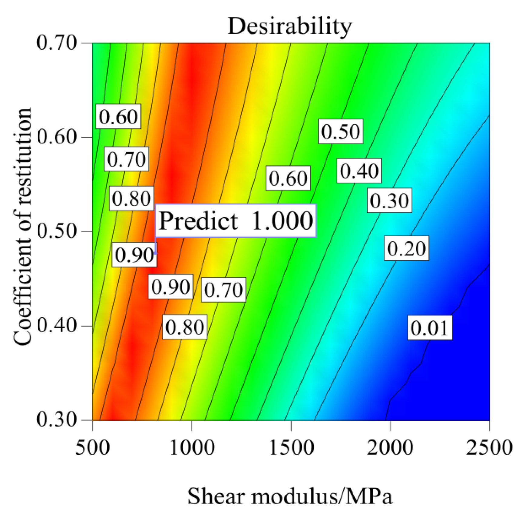
Parameter optimization for desirability
It can be seen from the above analysis that when the single index is used for calibration, the desirability of the predicted value can reach 1; when the dual-index is used for calibration, the desirability of the predicted value can reach more than 0.9, but no parameter combination reaches 1. The predicted values of the dual-index calibration are acoustic velocity = 517.0 m/s, dominant frequency = 17.5 kHz; the corresponding parameter combination is Poisson’s ratio 0.14, shear modulus 1663 MPa, coefficient of restitution 0.7, and the desirability level is 0.964. We conducted a univariate analysis of the model to analyze the reasons for the low desirability of dual-index calibration. And then to improve the desirability of dual-index co-calibration. The specific method is: to fix the horizontal coding value of two of the factors to 0 and find the regression equation of the dominant frequency Y1 and velocity Y2 and the coding value of a single factor, as shown in Equations (20)–(25):
Y 1 = 15.59 + 1.45 x 1
Y 1 = 15.59 + 5.74 x 2 1.38 x 2 2
Y 1 = 15.52 + 1.81 x 4
Y 2 = 571.3 + 63 . 76 x 1 + 18.39 x 1 2
Y 2 = 571.3 + 186.41 x 2 43.21 x 2 2
Y 2 = 571.3 63.2 x 4 + 11.71 x 4 2
Figure 7 and Figure 8 are the influence curves of various factors on the dominant frequency Y1 and the velocity Y2 of the acoustic wave. Comparing the two figures, we can see that with the increase of Poisson’s ratio (x1), the dominant frequency Y1 and the wave velocity Y2 both increase; with the increase of shear modulus (x2), the dominant frequency of acoustic wave Y1 and velocity Y2 all increase; with the increase of the coefficient of restitution (x4), the dominant frequency decreases, and the acoustic velocity Y2 increases. Univariate analysis shows that Poisson’s ratio (x1), shear modulus (x2) and coefficient of restitution (x4) had significant effects on the dominant frequency and wave velocity.
The above results show that the desirability of the predicted value cannot reach 1 when the two indexes are jointly calibrated. The reason is that after calibration, the predicted acoustic velocity of the model is greater than the actual acoustic velocity, and the predicted dominant frequency is smaller than the actual dominant frequency. Then it is necessary to reduce the acoustic velocity and increase the dominant frequency at the same time. It can be seen from the single factor analysis results (Figure 7 and Figure 8) that increasing the coefficient of restoration can reduce the acoustic velocity and increase the dominant frequency, so the range of the coefficient of restoration can be increased. We increased the coefficient of restitution from 0.3–0.7 to 0.3–0.8, resulting in a contour plot of desirability (Figure 9). Figure 9 shows that the desirability is increased to 1. At this time, the predicted value of dual-index calibration is acoustic velocity = 507 s, dominant frequency = 18 Hz, which is equal to the target value (index). Correspondingly, the parameter combination is Poisson’s ratio 0.3, shear modulus 1470 MPa, and collision recovery coefficient 0.79. It shows that the optimized parameters can make the calibration result reach the target value.
(2)
Validation of the optimal combination of parameters
This section verifies the optimal prediction results of two single and one dual index, respectively, and compares the three. The optimal parameter combination was obtained by the optimization module, with the actual measured acoustic wave dominant frequency of 18 kHz and acoustic velocity of 507 m/s as the target values (index). We inputted the above optimal parameter combination in the EDEM 2018 software (A software for discrete element simulation.) and conducted a simulation experiment to verify the optimization results. The optimal parameter combination, model prediction results, simulation verification results, and errors between the simulation and experimental results are shown in Table 10. The calculation method of the error between the simulation verification and the experimental result is shown in Equation (26).
erro = | simulation   verification   result - experimental   result experimental   result | × 100 %
It can be seen from the table that when the dominant frequency is used as the index. The errors between the simulation verification and the experimental results are as follows: the dominant frequency is 2.8%, and the velocity is 25.2%. The dominant frequency error of the acoustic wave is small, but the acoustic velocity error is significant, so the calibration result is poor. When the acoustic velocity is used as the index, the errors of the simulation verification and the measured results are, respectively, as follows: the dominant frequency of the acoustic wave is 35.6%, and the acoustic velocity is 0.14%. The dominant frequency error is small, but the velocity error is significant, so the calibration result is poor. In the case of dual-index calibration, the errors of simulation verification and experimental results are, respectively, as follows: the dominant frequency is 4.4%, and the acoustic velocity is 2.6%. The dominant frequency and velocity errors are minor, below 5%, within the acceptable range.
By observing the results of the two calibration methods, it can be seen that the single-index calibration can satisfy a single target well. However, the error between the other index and the experimental value may be significant. The dual-index calibration can limit the two indexes to a small range, significantly reducing the range of parameter values and improving the accuracy of the calibration.

4. Discussion

4.1. The Necessity of Constitutive Parameter Calibration

For granular bodies such as soil, only contact parameters are generally calibrated, while constitutive parameters such as Poisson’s ratio, shear modulus, and density are generally obtained by measurement. In this paper, the constitutive and contact parameters are given a range value by referring to the measured experiments, and then the parameters are calibrated. That is, we still use the parameter calibration method to determine the parameters that can be directly measured. It is determined by the complexity of the soil medium and the inconsistency between the discrete element simulated particles and the actual soil particles. Soil is a complex mixture of various substances, including other substances such as organic matter, and we cannot include all substances in the model. The properties of soil particles and aggregates of various substances can only be represented by a single particle in the simulation. The properties exhibited by this aggregate are undoubtedly different from the actual individual soil particles. Therefore, even if the parameters of actual soil particles can be obtained, the phenomena displayed in the simulation may be different from those in the experiment. At the same time, to reduce the calculation, the particle diameter is generally enlarged, and uniform particle size is used. However, the diameter distribution of actual soil particles is random. Mapping each particle with actual soil particles one-to-one in the simulation is impossible so the simulation results may differ from the experiment. Therefore, it is necessary to adjust the parameter values in a certain range through calibration and finally obtain the macroscopic properties of the soil material and, at the same time, reflect the particle characteristics.

4.2. Difference of Calibration Effect

Here we discuss the influence of different scenarios, different indexes, and the different number of indexes on the calibration effect. Rui et al. [31] calibrated the parameters of sandy soil particles with the angle of repose as the index by combining experiments and simulations. The results are Poisson’s ratio 0.3, shear modulus 1.15 × 10⁷, and soil—soil coefficient of restitution 0.15. Fei et al. [33] calibrated the soil parameters with the angle of repose as the index. The results are Poisson’s ratio 0.3, shear modulus 5 × 10⁷, and soil—soil coefficient of restitution 0.21. The above are all calibrated with the angle of repose as the index. However, the optimal parameter combination is different, especially the shear modulus, which is about four times the former. For the same medium (soil), the final calibration parameters should be the same or have a slight difference. The above are all calibrated with the angle of repose as the index. However, the optimal parameter combination is different, especially the shear modulus, which is about four times the former. For the same medium (soil), the final calibration parameter combination should be the same or have a slight difference. This is because the parameters that significantly impact the angle of repose are contacting parameters such as the coefficient of restitution, coefficient of static friction, and coefficient of rolling friction. In contrast, constitutive parameters such as shear modulus have no significant effect on the angle of repose. Therefore, significant changes in shear modulus do not significantly affect the angle of repose. The calibration results of Rui et al. [31] and Fei t al. [33] are also different from the results of this paper (Poisson’s ratio 0.3, shear modulus 1.407 × 10⁹ Pa, coefficient of restitution 0.79). It is because the indexes and the number of indexes are different in different scenarios, so the parameter combinations after calibration are different. Poisson’s ratio, shear modulus, and collision recovery coefficient significantly impact acoustic wave propagation, so these parameters must meet the two indexes of acoustic dominant frequency and velocity. Furthermore, other parameters that have no significant effect on acoustic wave propagation are not the focus of attention, and their values can be selected within a reasonable range. It is different from the parameters (coefficient of restitution, coefficient of static friction, and coefficient of rolling friction) that are focused on when calibrating the angle of repose. Therefore, the indexes and the number of indexes to be satisfied in different scenarios are different, and the calibrated parameter values may differ.
It can be seen from the above that the angle of repose calibration method cannot meet the requirements of all application scenarios and cannot be used as a widely applicable calibration method for all studies. Those calibrations that do not consider application scenarios have little reference to practical applications and appropriate calibration indexes should be selected according to the application scenarios. Of course, the method in this paper cannot satisfy all scenarios but can only satisfy the application of acoustic wave simulation. We consider that this phenomenon of inconsistent parameter values after calibration is acceptable. Those parameters that have no significant effect on the research purpose are allowed to have a certain difference from the parameters of the actual material, provided that these parameters are determined to have no or no significant effect on the research purpose.

5. Conclusions

In this research, the Hertz—Mindlin (no-slip) model was used to calibrate the parameters of the acoustic-soil propagation mode. Sensitivity analysis was carried out with the characteristic value of acoustic wave (acoustic velocity and dominant frequency) in the experiment as the calibration index to determine the parameters that significantly impact the acoustic velocity and dominant frequency. The sensitive parameters were optimized to obtain the optimal parameter combination. The following conclusions can be drawn:
(1)
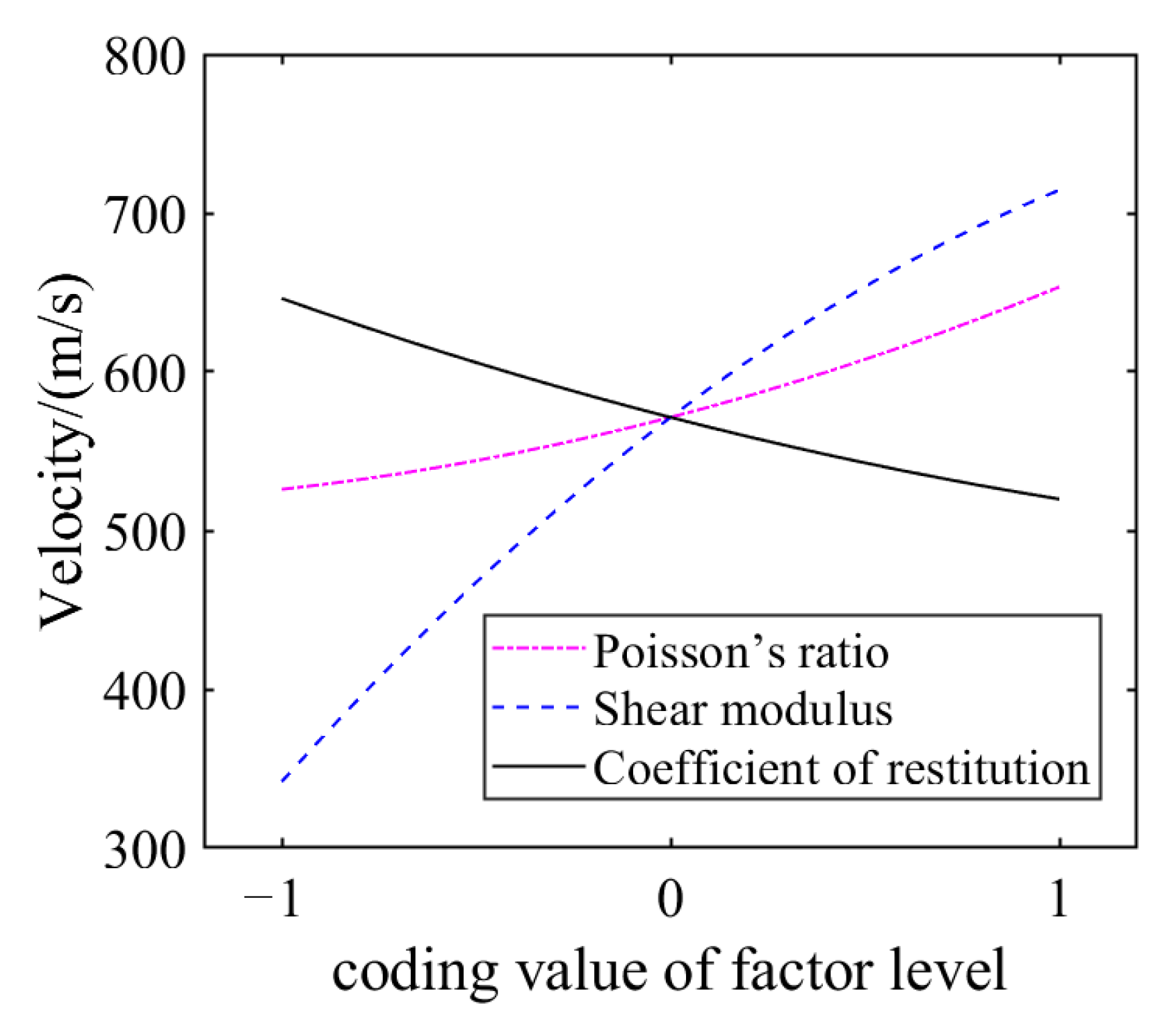
Based on EDEM software, the sensitivity analysis was carried out by the Plackett—Burman test. It was concluded that the sensitivity of each parameter to the dominant frequency of acoustic waves was ranked as Shear modulus, Poisson’s ratio, Coefficient of restitution, Coefficient of rolling friction, Density, and Coefficient of static friction. The order of sensitivity to acoustic velocity is Shear modulus, Poisson’s ratio, Coefficient of restitution, Coefficient of static friction, Coefficient of rolling friction, and Density.
(2)
Through the Box—Behnken test, the quadratic regression model of the three sensitive parameters on the dominant frequency and velocity is constructed and optimized. The optimal solutions of the two models are obtained as follows: shear modulus is 1407 MPa, Poisson’s ratio is 0.3, and coefficient of restitution is 0.79. The relative error values of the simulated dominant frequency and velocity and the actual values were 4.4% and 2.2%, respectively. It shows that the model constructed by the climbing test and the response surface test can well optimize the parameter values, and the optimal parameter combination can be used to study the acoustic wave propagation in the soil.
(3)
Comparing the calibration effect of the single and dual- indexes, it is found that a single index can only meet the calibrated index, while other indexes have significant errors. Moreover, the optional range of parameter values is wide and cannot be limited to a reasonable range. Dual-indexes can narrow the range of parameter values and meet the requirements of the two indexes. Therefore, the number of indexes should be increased as reasonably as possible to make the calibration effect more accurate and the parameter values more aligned with the actual materials.
(4)
The calibration of different scenarios is compared and discussed in this paper. It can be seen that the calibrated parameter combinations are different in different scenarios, so we should select the significant parameters according to the scenarios, then calibrate the significant parameters, and finally determine the final parameter combination.
This study provides a calibration method for building a model of acoustic propagation in soil. It can improve the accuracy of model construction and provide help for analyzing the interaction mechanism between soil and acoustic waves. This method can also select specific indexes according to the scene and apply it to the calibration of other materials.

Author Contributions

S.H.: Methodology, Writing—review and editing Data, Conceptualization, Investigation, curation. C.L.: Funding acquisition, Conceptualization, Methodology, Project administration, Supervision. H.L.: Methodology, Supervision Funding, acquisition, Conceptualization. J.H.: Conceptualization Supervision, Methodology. Q.W.: Conceptualization Supervision, Methodology. P.Y.: Data curation, Software. J.X.: Data curation, Software. S.J.: Data curation, Software. D.H.: Data curation, Software. All authors have read and agreed to the published version of the manuscript.

Funding

This work was funded by the Program for China Agriculture Research System of MOF and MARA (CARS-03), the 2115 Talent Development Program of China Agricultural University (2115) and the Chinese Universities Scientific Fund and Postgraduate Independent Innovation Research Fund Project of China Agricultural University (2022TC169), Innovative Research Team in University of China (IRT13039). Gratitude should be expressed to all the members of the Conservation Tillage Research Centre.

Conflicts of Interest

The authors declare that they have no known competing financial interests or personal relationships that could have appeared to influence the work reported in this paper.

References

  1. Xu, Y.; Li, J.; Duan, J.; Song, S.; Jiang, R.; Yang, Z. Soil water content detection based on acoustic method and improved Brutsaert’s model. Geoderma 2020, 359, 114003. [Google Scholar] [CrossRef]
  2. Dongqing, L.; Xing, H.; Feng, M.; Yu, Z. The impact of unfrozen water content on ultrasonic wave velocity in frozen soils. Procedia Eng. 2016, 143, 1210–1217. [Google Scholar] [CrossRef]
  3. Gorthi, S.; Chakraborty, S.; Li, B.; Weindorf, D.C. A field-portable acoustic sensing device to measure soil moisture. Comput. Electron. Agric. 2020, 174, 105517. [Google Scholar] [CrossRef]
  4. Weidinger, D.M.; Ge, L.; Stephenson, R.W. Ultrasonic Pulse Velocity Tests on Compacted Soil. In Proceedings of the Characterization, Modeling, and Performance of Geomaterials, Selected Papers from the 2009 GeoHunan International Conference, Changsha, China, 3–6 August 2009; pp. 150–155. [Google Scholar]
  5. Sarro, W.S.; Assis, G.M.; Ferreira, G.C.S. Experimental investigation of the UPV wavelength in compacted soil. Constr. Build. Mater. 2021, 272, 121834. [Google Scholar] [CrossRef]
  6. Lu, C.; Li, H.; He, J.; Wang, Q.; Wang, C.; Liu, J. A Preliminary Study of Seeding Absence Detection Method for Drills on the Soil Surface of Cropland Based on Ultrasonic Wave without Soil Disturbance. J. Sens. 2019, 2019, 7434197. [Google Scholar] [CrossRef]
  7. Otsubo, M.; Liu, J.; Kawaguchi, Y.; Dutta, T.T.; Kuwano, R. Anisotropy of elastic wave velocity influenced by particle shape and fabric anisotropy under K0 condition. Comput. Geotech. 2020, 128, 103775. [Google Scholar] [CrossRef]
  8. Huang, S.; Lu, C.; Li, H.; He, J.; Wang, Q.; Yuan, P.; Wang, Y. Transmission rules of ultrasonic at the contact interface between soil medium in farmland and ultrasonic excitation transducer. Comput. Electron. Agric. 2021, 190, 106477. [Google Scholar] [CrossRef]
  9. Roessler, T.; Richter, C.; Katterfeld, A.; Will, F. Development of a standard calibration procedure for the DEM parameters of cohesionless bulk materials–part I: Solving the problem of ambiguous parameter combinations. Powder Technol. 2019, 343, 803–812. [Google Scholar] [CrossRef]
  10. Richter, C.; Roessler, T.; Kunze, G.; Katterfeld, A.; Will, F. Development of a standard calibration procedure for the DEM parameters of cohesionless bulk materials–Part II: Efficient optimization-based calibration. Powder Technol. 2020, 360, 967–976. [Google Scholar] [CrossRef]
  11. Li, P.; Ucgul, M.; Lee, S.H.; Saunders, C. A new approach for the automatic measurement of the angle of repose of granular materials with maximal least square using digital image processing. Comput. Electron. Agric. 2020, 172, 105356. [Google Scholar] [CrossRef]
  12. Wensrich, C.M.; Katterfeld, A. Rolling friction as a technique for modelling particle shape in DEM. Powder Technol. 2012, 217, 409–417. [Google Scholar] [CrossRef]
  13. Benvenuti, L.; Kloss, C.; Pirker, S. Identification of DEM simulation parameters by Artificial Neural Networks and bulk experiments. Powder Technol. 2016, 291, 456–465. [Google Scholar] [CrossRef]
  14. Do, H.Q.; Aragón, A.M.; Schott, D.L. A calibration framework for discrete element model parameters using genetic algorithms. Adv. Powder Technol. 2018, 29, 1393–1403. [Google Scholar] [CrossRef]
  15. Alonso-Marroquín, F.; Ramírez-Gómez, Á.; González-Montellano, C.; Balaam, N.; Hanaor, D.A.H.; Flores-Johnson, E.A.; Shen, L. Experimental and numerical determination of mechanical properties of polygonal wood particles and their flow analysis in silos. Granul. Matter 2013, 15, 811–826. [Google Scholar] [CrossRef]
  16. Marigo, M.; Stitt, E.H. Discrete element method (DEM) for industrial applications: Comments on calibration and validation for the modelling of cylindrical pellets. KONA Powder Part. J. 2015, 32, 236–252. [Google Scholar] [CrossRef]
  17. Coetzee, C.J.; Els, D.N.J. Calibration of discrete element parameters and the modelling of silo discharge and bucket filling. Comput. Electron. Agric. 2009, 65, 198–212. [Google Scholar] [CrossRef]
  18. Combarros, M.; Feise, H.J.; Zetzener, H.; Kwade, A. Segregation of particulate solids: Experiments and DEM simulations. Particuology 2014, 12, 25–32. [Google Scholar] [CrossRef]
  19. Li, Q.; Feng, M.; Zou, Z. Validation and calibration approach for discrete element simulation of burden charging in pre-reduction shaft furnace of COREX process. ISIJ Int. 2013, 53, 1365–1371. [Google Scholar] [CrossRef]
  20. Nakashima, H.; Shioji, Y.; Kobayashi, T.; Aoki, S.; Shimizu, H.; Miyasaka, J.; Ohdoi, K. Determining the angle of repose of sand under low-gravity conditions using discrete element method. J. Terramech. 2011, 48, 17–26. [Google Scholar] [CrossRef]
  21. Zhanhua, S.O.N.G.; Hao, L.I.; Yinfa, Y.A.N.; Fuyang, T.I.A.N.; Yudao, L.I.; Fade, L.I. Calibration Method of Contact Characteristic Parameters of Soil in Mulberry Field Based on Unequal-diameter Particles DEM Theory. Trans. Chin. Soc. Agric. Mach. 2022, 53, 21–33. [Google Scholar]
  22. Shen, H.H.; Zhang, H.; Fan, J.K.; Xu, R.Y.; Zhang, X.M. A rock modeling method of multi-parameters fitting in EDEM. Rock Soil Mech. 2021, 42, 2298–2310. [Google Scholar] [CrossRef]
  23. Cundall, P.A.; Strack, O.D. A discrete numerical model for granular assemblies. Geotechnique 1979, 29, 47–65. [Google Scholar] [CrossRef]
  24. Di Renzo, A.; Di Maio, F.P. Comparison of contact-force models for the simulation of collisions in DEM-based granular flow codes. Chem. Eng. Sci. 2004, 59, 525–541. [Google Scholar] [CrossRef]
  25. Huang, S.; Lu, C.; Li, H.; He, J.; Wang, Q.; Gao, Z.; Yuan, P.; Li, Y. The attenuation mechanism and regular of the acoustic wave on propagation path in farmland soil. Comput. Electron. Agric. 2022, 199, 107138. [Google Scholar] [CrossRef]
  26. Rianyoi, R.; Potong, R.; Ngamjarurojana, A.; Chaipanich, A. Mechanical, dielectric, ferroelectric and piezoelectric properties of 0–3 connectivity lead-free piezoelectric ceramic 0.94 Bi0. 5Na0. 5TiO3–0.06 BaTiO3/Portland cement composites. J. Mater. Sci. Mater. Electron. 2021, 32, 4695–4704. [Google Scholar] [CrossRef]
  27. Jiang, F. Research on the Piezoelectric Ultrasonic Nebulizer. Master’s Thesis, Nanjing University of Aeronautics and Astronautics, Nanjing, China, 2014. [Google Scholar]
  28. Ucgul, M.; Fielke, J.M.; Saunders, C. 3D DEM tillage simulation: Validation of a hysteretic spring (plastic) contact model for a sweep tool operating in a cohesionless soil. Soil Tillage Res. 2014, 144, 220–227. [Google Scholar] [CrossRef]
  29. Ucgul, M.; Saunders, C.; Fielke, J.M. Discrete element modelling of tillage forces and soil movement of a one-third scale mouldboard plough. Biosyst. Eng. 2017, 155, 44–54. [Google Scholar] [CrossRef]
  30. Shi, L.; Zhao, W.; Sun, W. Parameter calibration of soil particles contact model of farmland soil in northwest arid region based on discrete element method. Trans. Chin. Soc. Agric. Eng. 2017, 33, 181–187. [Google Scholar]
  31. Rui, Z.; Dianlei, H.A.N.; Qiaoli, J.I.; Yuan, H.E.; Jianqiao, L.I. Calibration methods of sandy soil parameters in simulation of discrete element method. Nongye Jixie Xuebao/Trans. Chin. Soc. Agric. Mach. 2017, 48, 49–56. [Google Scholar]
  32. Huang, Y.; Hang, C.; Yuan, M.; Wang, B.; Zhu, R. Discrete element simulation and experiment on disturbance behavior of subsoiling. Trans. CSAM 2016, 47, 80–88. [Google Scholar]
  33. Dai, F.; Song, X.; Zhao, W.; Zhang, F.; Ma, H.; Ma, M. Simulative calibration on contact parameters of discrete elements for covering soil on whole plastic film mulching on double ridges. Nongye Jixie Xuebao/Trans. Chin. Soc. Agric. Mach. 2019, 50, 49–56. [Google Scholar]
Figure 1. Acoustic−soil test bench.
Remotesensing 15 00943 g001
Figure 2. DEM model. (a) 3D model; (b) Side view and acoustic wave propagation process.
Remotesensing 15 00943 g002
Figure 3. Fourier transform of the received signal. (a) Time—domain signal; (b) Frequency—domain signal.
Remotesensing 15 00943 g003
Figure 4. Desirability contour map dominant frequency as an indicator.
Remotesensing 15 00943 g004
Figure 5. Desirability contour map velocity as indicator.
Remotesensing 15 00943 g005
Figure 6. Desirability contour map dominant frequency and velocity as indicators.
Remotesensing 15 00943 g006
Figure 7. Curves of various factors on the dominant frequency.
Remotesensing 15 00943 g007
Figure 8. Curves of various factors on the velocity.
Remotesensing 15 00943 g008
Figure 9. Contour plot of desirability with the coefficient of restitution 0.3–0.8.
Remotesensing 15 00943 g009
Table 1. Physical parameters.
ObjectPoisson’s RatioShear Modulus (MPa)Density (kg/m3)
steel0.257.9 × 10107860
pzt0.327.5 × 10107900
Table 2. Contact parameters.
ObjectCoefficient of
Restitution
Coefficient of
Static Friction
Coefficient of
Rolling Friction
soil–steel0.50.50.05
soil–pzt0.50.40.04
Table 3. Factors and Levels of simulation test.
FactorLevel
−11
X1/Poisson’s ratio0.050.45
X2/Shear modulus (MPa)5002500
X3/Density (kg/m3)16503650
X4/Coefficient of restitution0.30.7
X5/Coefficient of static frisction0.30.7
X6/Coefficient of rolling friction0.150.35
Table 4. Factors and levels of the Box—Behnken experimental.
Factors and
Levels
Poisson’s RatioShear Modulus (MPa)Coefficient of Restitution
−10.055000.3
00.2515000.5
10.4525000.7
Table 5. Design and results of Plackett—Burman experiments.
No.Experimental LevelDominant Frequency
Y1 (kHz)
Acoustic
Velocity
Y2 (m/s)
A1A2A3A4A5A6
1−1111−1−122.2563.4
211−1−1−1120.0888.9
3−111−11116.4727.3
41−111−1111.5350.9
51−1111−111.1354
611−111123.3754.7
7111−1−1−123.3754.7
8−1−11−1116.8347.8
9−1−1−11−118.7289.9
101−1−1−11−18.6434.8
11−11−111−120.0606.1
12−1−1−1−1−1−16.8363.6
Table 6. Analysis of variance of Plackett—Burman experiment.
Source of
Variance
Dominant Frequency/Y1Acoustic Velocity/Y2
Sum of
Squares
dfMean
Square
FpSum of
Squares
dfMean Sum
of Square
Fp
Model477.62679.6062.150.00024.621 × 105677,015.33104.12<0.0001
X123.80123.8018.580.007634,122.67134,122.6746.130.0011
X2428.411428.41334.48<0.00013.867 × 10513.86 × 105522.75<0.0001
X31.2711.270.990.36554796.0014796.006.480.0515
X418.50118.5014.440.012629,810.30129,810.3040.300.0014
X53.3113.312.580.169014.74114.740.0200.8932
X62.3412.341.830.23436669.3716669.379.020.0300
Residual6.4051.28 3698.335739.71
Cor Total484.0311 4.658 × 10511
Table 7. The results of the sensitivity analysis.
ParametersDominant Frequency/Y1Acoustic Velocity/Y2
Standardization
Effect
Mean Sum
of Square
Contribution
Degree/%
Standardization
Effect
Mean Sum
of Square
Contribution
Degree (%)
X12.8223.804.92106.6534,122.77.33
X211.95428.4188.51359.02386,67983.02
X30.651.270.26−9.9847961.03
X42.4818.513.82−9.6829,810.306.40
X5−1.053.310.682.2214.740.003
X6−0.882.340.4847.156669.371.43
Table 8. The design scheme and results of Box-Behnken.
No.Factor Level ValueDominant
Frequency
Y1 (kHz)
Acoustic
Velocity
Y2 (m/s)
X1X2X4
1−1−107.5315.2
21−109.3404
3−11017.9666.7
411022.2800.0
5−10−112.5588.2
610−115.2740.7
7−10116.1470.6
810118.9606.1
90−1−17.3400
1001−117.5806.3
110−119.8307.7
1201122.2645.2
1300015.6571.4
1400015.2579.6
1500015.9565.1
1600015.3575.6
1700015.6564.8
Table 9. ANOVA of Box—Behnken design quadratic model.
Source of
Variance
Dominant Frequency/Y1Acoustic Velocity/Y2
Sum of
Squares
Free-
Dom
Mean SquareFpSum of
Squares
Free-
Dom
Mean SquareFp
Model317.31935.26593.97<0.00013.536 × 105939,293.07385.86<0.0001
X116.82116.82283.37<0.000132,525.25132,525.25319.40<0.0001
X2263.351263.354436.72<0.00012.78 × 10512.78 × 1052729.96<0.0001
X426.28126.28442.76<0.000131,953.92131,953.92313.79<0.0001
X1X21.5611.5626.320.0014495.061495.064.860.0633
X1X42.5 × 10−312.5 × 10−30.0420.843272.25172.250.710.4274
X2X41.2111.2120.390.00271183.3611183.3611.620.0113
X120.03410.0340.570.47321423.5811423.5813.980.0073
X228.0818.08136.07<0.00017862.4017862.4077.21<0.0001
X420.01810.0180.300.6011577.611577.615.670.0488
Residual0.4270.059 712.827101.83
Lack of Fit0.1130.0360.470.7221544.743181.584.320.0957
Pure Error0.3140.077 168.08442.02
Cor Total317.7216 3.544 × 10516
Table 10. Model prediction optimal parameter combination, prediction results, simulation verification results and errors between simulation verification and experimental results.
Optimization Index Type (Target Value)Dominant Frequency (18 kHz)Acoustic Velocity (507 m/s)Dominant Frequency (18 kHz)
Acoustic Velocity (507 m/s)
Optimal parameter combination of fitting model predictionPoisson’s ratio0.250.090.3
Shear Modulus (MPa)183611651407
Coefficient of restitution0.560.370.79
Fitting model prediction Dominant frequency (kHz)18/18
Acoustic velocity (m/s)/507507
Simulation verification Dominant frequency (kHz)17.511.617.2
Acoustic velocity (m/s)634.9506.3493.8
Error between simulation verification and experimental Dominant frequency (%)2.8035.604.4
Acoustic velocity (%)25.200.142.60
Disclaimer/Publisher’s Note: The statements, opinions and data contained in all publications are solely those of the individual author(s) and contributor(s) and not of MDPI and/or the editor(s). MDPI and/or the editor(s) disclaim responsibility for any injury to people or property resulting from any ideas, methods, instructions or products referred to in the content.

