
Auto-Diagnosis of Time-of-Flight for Ultrasonic Signal Based on Defect Peaks Tracking Model

1
Department of Electrical Engineering, The Hong Kong Polytechnic University, Hong Kong
2
School of Design, The Hong Kong Polytechnic University, Hong Kong
3
Centre for Medical and Industrial Ultrasonics, James Watt School of Engineering, University of Glasgow, Glasgow, Scotland G12 8QQ, UK
*
Author to whom correspondence should be addressed.
Remote Sens. 2023, 15(3), 599; https://doi.org/10.3390/rs15030599
Submission received: 15 December 2022
/
Revised: 2 January 2023
/
Accepted: 17 January 2023
/
Published: 19 January 2023
(This article belongs to the Special Issue Remote Sensing in Structural Health Monitoring)
Abstract
:With the popularization of humans working in tandem with robots and artificial intelligence (AI) by Industry 5.0, ultrasonic non-destructive testing (NDT)) technology has been increasingly used in quality inspections in the industry. As a crucial part of handling ultrasonic testing results–signal processing, the current approach focuses on professional training to perform signal discrimination but automatic and intelligent signal optimization and estimation lack systematic research. Though the automated and intelligent framework for ultrasonic echo signal processing has already exhibited essential research significance for diagnosing defect locations, the real-time applicability of the algorithm for the time-of-flight (ToF) estimation is rarely considered, which is a very important indicator for intelligent detection. This paper conducts a systematic comparison among different ToF algorithms for the first time and presents the auto-diagnosis of the ToF approach based on the Defect Peaks Tracking Model (DPTM). The proposed DPTM is used for ultrasonic echo signal processing and recognition for the first time. The DPTM using the Hilbert transform was verified to locate the defect with the size of 2–10 mm, in which the wavelet denoising method was adopted. With the designed mechanical fixture through 3D printing technology on the pipeline to inspect defects, the difficulty of collecting sufficient data could be conquered. The maximum auto-diagnosis error could be reduced to 0.25% and 1.25% for steel plate and pipeline under constant pressure, respectively, which were much smaller than those with the DPTM adopting the cross-correlation. The real-time auto-diagnosis identification feature of DPTM has the potential to be combined with AI in future work, such as machine learning and deep learning, to achieve more intelligent approaches for industrial health inspection.
1. Introduction
With the aging of urban buildings, the demand for automated non-destructive testing (NDT) of pipelines and facilities is increasing [1,2], leading to the increasing amount and complexity of data [1]. Among the NDT techniques, ultrasound is one of the cost-effective inspection technologies. Nevertheless, the current method used in the industry is still mainly based on manual identification, which requires high professional skills for operation and analysis [3,4,5,6]. Manual data identification could lead to data inconsistencies, especially in the case of a large amount of complex data [7]. Thus, automated NDT systems with high reliability are desired [7,8,9].
Urban underground pipelines are divided into natural gas pipelines, sewage pipelines, water pipelines, gas pipelines, heat pipelines, oil and gas pipelines, industrial pipelines, etc. [10]. The pipelines are continuously eroded by corrosive liquids or gases over the years, leading to the structural weakening of the pipeline and the high possibility of deformation and fracture [10,11]. In addition, due to subjective factors, the operators may misjudge the position and dimensions of defects, resulting in the accumulation of hidden safety hazards in pressure pipelines [12,13]. Therefore, NDT would be an indispensable part of pipeline maintenance in the future.
Based on the propagation and reflection of acoustic waves, the ultrasonic inspection can detect the size, nature, and location of internal defects in the target material. In general, there are two categories of inspection methods depending on how the waves are transmitted and received: (1) transmit the wave using an ultrasonic transducer while receiving the signal using the other one [14,15]; (2) detect and receive the signal using the same ultrasonic transducer [14,15].
There are many types of ultrasonic transducers such as a straight transducers, angular transducers, curvature transducers, surface wave transducers, double crystal transducers, high-temperature transducers, etc. [15,16]. The probe used in this work was a single-chip vertical 5-MHz ultrasonic probe, which generated the longitudinal wave perpendicular to the target surface [16]. Researchers have studied and compared the transducers in terms of center frequency and materials for pipe detection. However, there is a lack of sufficient research on how to process the pipeline echo data in real time. Signal processing is crucial for extracting useful information from the raw data in either the time domain or frequency domain [17,18].
The intelligence in NDT—radiographic testing (RT), ultrasonic testing (UT), magnetic particle testing (MT), and liquid penetrant testing (PT)—is gradually becoming a future trend with the proposal of Industry 5.0. The earliest research was performed from the perspective of the classification of defect categories. The image processing combined with artificial neural networks was proposed and successfully applied to the RT-based method on welds [19]. With the advancement of deep learning and equipment, convolutional neural networks are applied to analyze signals by the specific film scanner to acquire images for industrial and medical applications, in which optimized recognition of images based on deep learning would be the focus of research [7]. The research on intelligence in MT was proposed in 1994. An analog VLSI architecture combined with neural networks for image processing was implemented and validated in the industry; nevertheless, the combination with other imaging devices became a necessary precondition such as cameras according to the imaging limitations of MT [20]. Since the technology of magnetic particle imaging (MPI) was introduced in 2005, reconstruction algorithms based on voltage-response signal imaging have become a hot research topic [21,22,23]. Improvements in the accurate models for system matrix (SM)-based and x-space-based algorithms combined with deep learning are the focus of future research [24,25,26]. The PT approach relies heavily on the penetrant and manual operation, so there has still been relatively little research on the intelligence in LT [27]. The intelligence of UT is mainly divided into the intelligent design of ultrasonic transducer and the intelligent processing of imaging and signals. The neural network model and modified particle swarm optimization algorithm were applied for the optimization of ultrasonic transducer matching layer thickness and the quantitative effect of the matching layer on the transducer performance [28]. The selection of the matching layer material and the effect of the transducer structure on the evaluation of the application performance based on neural network models will be one of the future development directions [29,30]. Ultrasound image and signal processing have always been the focus of optimization. The approach of combining neural networks for ultrasonic NDT was first proposed in 1999, however, it could only be used to assist in identifying the type of defect on the steel plate [31]. The classifications of porosity, unfused, tungsten inclusions, and non-defects were achieved after being implemented by combining wavelet filtering with backpropagation neural networks [31]. Artificial intelligence (AI) with a novel code containing a decision tree was proposed and verified for characterizing single large planar cracks recently, which demonstrated the feasibility of explainable AI in industrial NDE [32]. A new approach for locating defects by inputting the probability matrix of ToF into a neural network for training as an input layer has been proposed, but the accuracy was not good enough to be applied in practical engineering with fuzzy probability and the uncertainty of neural networks [33]. Subsequently, image and signal optimization for ultrasonic detection combined with deep learning has become a trend [34,35,36].
Overall, neural networks are essentially nonlinear optimization algorithms with uncertainty such that the combination of neural networks and ultrasonic NDT would sacrifice the localization accuracy of detection in the absence of a large amount of training data, making it difficult to apply to real applications [36,37,38]. Thus, the accuracy of defect positioning in the current approaches needs to be improved. There is still a lack of in-depth research on the accuracy improvement of automatic extraction and identification for signals, which is essential for the intelligent application of ultrasonic NDT.
This paper presents and implements the cross-correlation method, the threshold detection method, and the envelope method in detail, which provides a comprehensive perspective for later studies and thus accelerate the research progress about the intelligent NDT. This work investigates how to detect and locate the defects of the pipeline automatically based on signal processing technology. In this study, intelligent thickness estimation without a preset range is achieved for the first time by conducting the auto-diagnosis of the core parameter, ToF, in ultrasonic inspection with high accuracy. Combined with the proposed defect peaks tracking model (DPTM), the auto-diagnosis of ToF estimation is achieved without setting the thickness range in advance based on the Hilbert transform and wavelet filtering. With the proposed approach, higher accuracy is realized when compared to the conventional method, with errors of 1.25% and 0.25% for pipelines and 304SS, respectively. The proposed approach does not have strict specific requirements of hardware devices compared to the conventional method.
In this paper, Section 2 introduces the experimental equipment designed to validate the proposed method. Section 3 describes the DPTM for the auto-diagnosis of ToF. Section 4 verifies the accuracy of the proposed approach based on the DPTM experimentally and demonstrates the feasibility of the defective pipeline. Section 5 discusses the strengths and weaknesses of the approach. Section 6 summarizes the research and provides a prospect for future work.
2. Experimental
In this section, the devices and approaches used to acquire the data for defect detection are described. To ensure the reliability of data acquisition, a pulser–receiver, CTS-9009PLUS (Shantou Institute of Ultrasonic Instruments Co., Ltd., Shantou, Guangdong, China), with a sampling rate of 264 MHz was employed to guarantee the signal integrity and meet the requirements of signal processing.
2.1. Transducer Fixture
A 5-MHz transducer fixture shown in Figure 1 was designed for structural health monitoring of pipelines, which was a standard single-element crystal probe for vertical flaw inspection consisting of the piezoelectric wafer, sound-absorbing material, metal housing, etc. The overall size of the fixture was 94.5 mm × 51.5 mm × 51.5 mm. The fixture was designed to fix the ultrasonic transducer on a lifting arm and optimize the surface-fitting conditions, which could adapt to an inclined surface and provide a controllable pressing force to the transducers.
The fixture was mainly constructed in three PLA 3D-printed parts: a container, a base, and a housing. The container held the transducer, and the housing was fixed on the lifting arm. The container, a compression spring, and a base were assembled into the housing in order, and then the base was locked at the assigned position in the housing with screws and nuts. As the housing limits the movement of the container, the spring was in compression. A narrow chamber was designed to allow little movement of the container, in which the transducer could tilt with a maximum of 10° against the inclined surface and an altitude mismatch of ±4 mm against the lifting arm.
The pressing force could be adjusted by the specifications of the spring. A steel alloy spring with a free length of 40 mm and a spring rate of 2.0 N/mm was selected for this work to ensure full contact between the transducer and the testing object. The fixture was tuned to provide a pressing force of 50 ± 8 N.
2.2. Data Acquisition
The experimental settings for ultrasonic signal detection in the pipeline are shown in Figure 2. Cast iron pipes are widely used in water supply and drainage due to their excellent anticorrosion performance, good ductility, and good sealing effect [19,20]. Therefore, the cast iron pipeline was adopted in this work. The wall thickness and radius of the pipeline were 7 mm and 170 mm, respectively. The pulser–receiver (CTS-9009PLUS) was used to trigger the ultrasonic transducer that was in contact with the inner surface of the pipeline and collect the data from the transducer. Matlab R2021a was used to process the signal. The measurements were taken multiple times at each point, while data processing and estimation results were displayed in real-time.
3. Defect Peaks Tracking Model (DPTM)
The DPTM adopted the Hilbert transform, the envelope method, and the quadratic spline interpolation for the first time, which realized the automatic estimation of the time-of-flight (ToF) signal. DPTM enables auto-diagnosis through signal eigenvalues to accurately estimate ToF, which is of great significance for the realization of Industry 5.0.
3.1. ToF Estimation Algorithm
Nowadays, the manufacturing industry tends to be automated. As an important means for structural health monitoring, ultrasonic NDT should also be evolved into intelligent and automated technology [39,40]. ToF is a key parameter in ultrasonic NDT for damage detection, which will be elaborated on in this section [39]. Though there have been quite a few methods for the ToF determination, the ultrasonic signal estimation algorithm has not been optimized for industrial health monitoring.
Conventional methods for determining the ToF collected from the transducer include the cross-correlation method, the threshold detection method, and the envelope method [41]. The ToF evaluation processes are shown in Figure 3.
The cross-correlation algorithm determines the ToF by estimating the similarity of echo signals from two individual transducers, which is currently the most widely used method to measure the relative time delay of two ultrasonic transducers [42,43]. Nevertheless, the cross-correlation algorithm is easily affected by the noise and reverberation environment such that the requirements on the instrument are strict for processing the real-time estimation [44]. In real applications, a single transducer for NDT would be preferred in terms of cost and flexibility. This work realizes the cross-correlation ToF estimation using a single ultrasonic probe by the DPTM for the first time.
and represent the signal needed to be compared, where and represent the average value of and . is the correlation among representative signals, such that the ToF between and can be calculated when reaches the maximum. The core formulas of the cross-correlation algorithm is shown as Equations (1) and (2).
The threshold detection method is to detect specific echo signals by setting a threshold voltage [39,45,46]. Its advantage is a simple operation, but the detectable ranges of defects and thicknesses are limited [47]. Though there have been many threshold methods such as the dynamic threshold method, double threshold method, and variable ratio threshold method [47], noise can easily affect the received echo signal threshold, and the adjustment of gain also determines the voltage threshold with great uncertainty [48]. Since the measured ToF would change along with the measurement conditions, the intensity of the ultrasonic echo signal would also change. Therefore, it is not realistic to set a certain threshold value in the real ultrasonic measurement process [45].
The envelope method is to take the envelope of the signal employing interpolation, which is easy to find the peak value and calculate the ToF [49]. However, the echo signal processed by the envelope usually encounters the loss of part of the original data information. To resolve the problem, the present work employs the machine learning approach to learn the characteristics of the original signal, process the signal through the Hilbert transform, and estimate the accuracy of the pipeline defect detection algorithm by connecting the transducer in real time.
3.2. Hilbert Transform in Defect Peaks Tracking Model (DPTM)
Empirical mode decomposition (EMD) can decompose multiple intrinsic mode functions (IMFs) from low frequency to high frequency from the signal x(t) [50].
where is a residual function representing the average changing trend of the signal, and is an IMF, containing components at different temporal feature scales of the signal. Hilbert transform is performed on the IMF component and the instantaneous parameter spectrum of the signal can be obtained as follows:
An analytical signal can be constructed as follows, which only involves the positive frequency part from the frequency domain:
Each IMF component corresponds to the following equation the Hilbert transform:
means to take the real part, and the reason for omitting the residual function is that the residual function mainly represents the average changing trend of the signal, which has no effect on the frequency characteristics of the signal. represents the instantaneous frequency. The Hilbert amplitude spectrum is:
Since the function of EMD is to decompose the parts with different frequencies in the original signal, the timing for when to perform EMD decomposition on the signal plays a crucial role in the accuracy of the final signal. In this work, the best time of EMD processing in the actual ultrasonic signal estimation is compared and discussed, and the obtained results are compared with the signal without involving the processing of EMD. The Hilbert transform is applied for achieving both the acquisition of the single-sided spectrum and the integrity of the signal information.
In addition, wavelet denoising was used to reduce noise interference during the measurement process. Based on the wavelet decomposition, the signal and noise show different characteristics at different scales—as the scale increases, the wavelet coefficients of the actual signal and noise would gradually increase. In the practical application of defect detection, in addition to removing the noise interference in the signal, the denoising algorithm also needs to preserve the singularity of the fault signal. In contrast to the Fourier transform using an infinitely long trigonometric function as the basis, the wavelet transform adopts a finite-length decaying wavelet basis as follows:
where represents the signal obtained after wavelet filtering, and and are scale and translation, respectively. The scale controls the scaling of the wavelet function, while the translation controls the translation of the wavelet function. represents the wavelet base.
3.3. Ultrasonic Signal Smoothing Algorithm in DPTM
Signal smoothing will be a crucial step to obtain accurate ToF results in fully automatic and intelligent ultrasonic inspection systems in the future. In the process of real-time intelligent estimation, fewer glitches and oscillations could reduce the probability of errors. This work compares quadratic spline interpolation and cubic spline interpolation for intelligent calculation.
After obtaining the Hilbert-transformed envelope, there are still glitches in the envelope. The spline interpolation method for smoothing curves is the first option for processing in Equation (6). On a given signal interval , a function is a spline function that satisfies the following equations:
where is the power function, which is a unit jump function when .
The value at the critical point during the auto-diagnosis process would cause serious distortion of the signal and make the ToF estimation inaccurate. Thus, the smoothing step by the interpolation method is necessary for reducing the error.
To simplify the calculation process and achieve a better filtering effect, the quadratic spline interpolation algorithm is adopted in this work using the polynomial least squares method to approximate the sampling points shown as Equations (15)–(18).
The cubic spline interpolation is suitable for processing both time domain and frequency domain signals. The smoothing method of time domain data can reduce the mixing of high-frequency random noise and vibration signals, which also converts the frequency domain data into smooth spectral curves to suit the needs of modal parameter identification. The cubic spline interpolation algorithm is as follows:
The purpose of DPTM (Figure 4) is to speed up the estimation process and reduce the estimation error rate. Therefore, the following core formulas were designed to find peaks and reduce errors in DPTM:
where represents the sampling time points found based on the voltage peak point , and represent the sampling time points and the voltage values of adjacent peaks according to the sorting coefficient , respectively, represents the correction factor, which is the number ToF values, e is the minimum time error of sampling that is used to judge whether the final calculated value is reasonable, and represents the sampling frequency. If the final value is less than , the value will be removed from the final averaged sum calculated by Equation (22).
Figure 4 shows the flowchart of the DPTM process, in which wavelet denoising was used to remove noise from the signal so that the denoised signal will not produce “Mode mixing” during the EMD decomposition of the signal at different frequencies. The Hilbert transform was then used to simplify the signal in the time and frequency domains, and the smoothing algorithm was used to smooth the signal and thus reduce the error of auto-diagnosis. Finally, the system automatically would compare the errors and determine the final ToF value according to Equations (22)–(24). Figure 5 shows the flow chart of the adjustable defect estimation algorithm based on the DPTM. CTS-9009PLUS will be controlled and excited by the computer through TCP/IP protocol in real time. The ultrasonic echo data was processed by wavelet filtering, the Hilbert transform, then smoothing by the interpolation method will be performed, and finally, the estimation result will be obtained by DPTM.
The DPTM is proposed and applied to the estimation of ToF for the first time, which can improve the accuracy of estimation results and avoid serious estimation errors. However, the DPTM lacks autonomous learning capability when the signal is seriously overwhelmed by noise for intelligent detection. Thus, future work is to address the shortcoming of the Backpropagation (BP) neural network.
4. Results
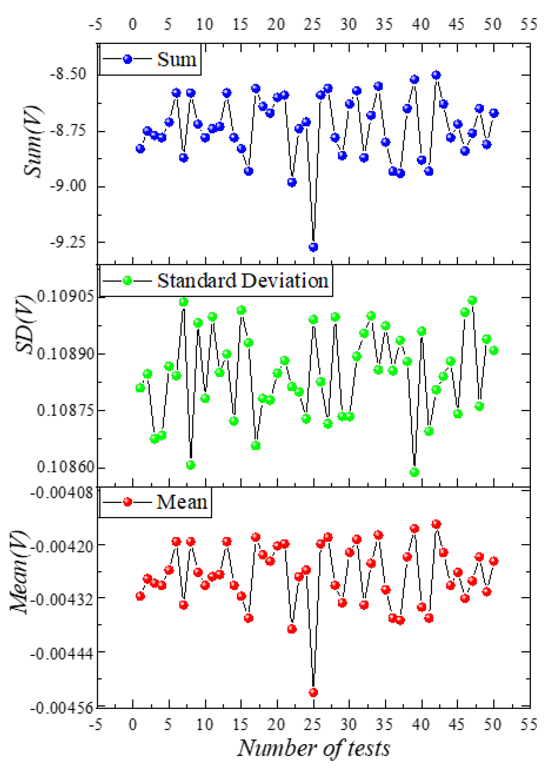
A 10 mm-thick plate made of 304 stainless steel (304SS) was used for the basic performance evaluation of the proposed DPTM. Linear regression was used for the calibration of the longitudinal acoustic velocity of 304SS (5978 m/s). To ensure the intelligent real-time ToF estimation of the algorithm, the calculation process should abandon the manual signal-selection process. Instead, all the algorithm programs should be run automatically by Matlab programs. Figure 6 shows an example of 50 sets of data obtained under constant pressure with a pulse voltage of 300 V and a pulse width of 200 ns and a gain of 60 dB to verify the algorithm. Fifty sets of data should be good enough for verification because of having subtle differences due to the instrument sampling rate and noise. The statistics of ultrasonic echo signals are shown in Figure 7, showing that even slight changes in the signal could be captured. The horizontal axis in Figure 7 represents the number of single-point tests, while the vertical axes represent the standard deviation (SD), sum and mean of the echo data, respectively, collected each time.
To explore the influence of EMD on the estimation of target thickness, 50 sets of ultrasonic echo signals obtained at the 10mm position of the steel plate were analyzed by the following algorithms: Hilbert and EMD analyzed the signals in different orders, while wavelet and Hilbert analyzed and processed the signals, and the cross-correlation method was used for signal analysis and processing in the frequency domain. In order to achieve fully automatic real-time estimation, all these algorithms were performed using the DPTM. At the same time, this is also the first time to realize the real-time intelligent ToF estimation by cross-correlation method in the transmitting-receiving mode of a single ultrasonic probe.
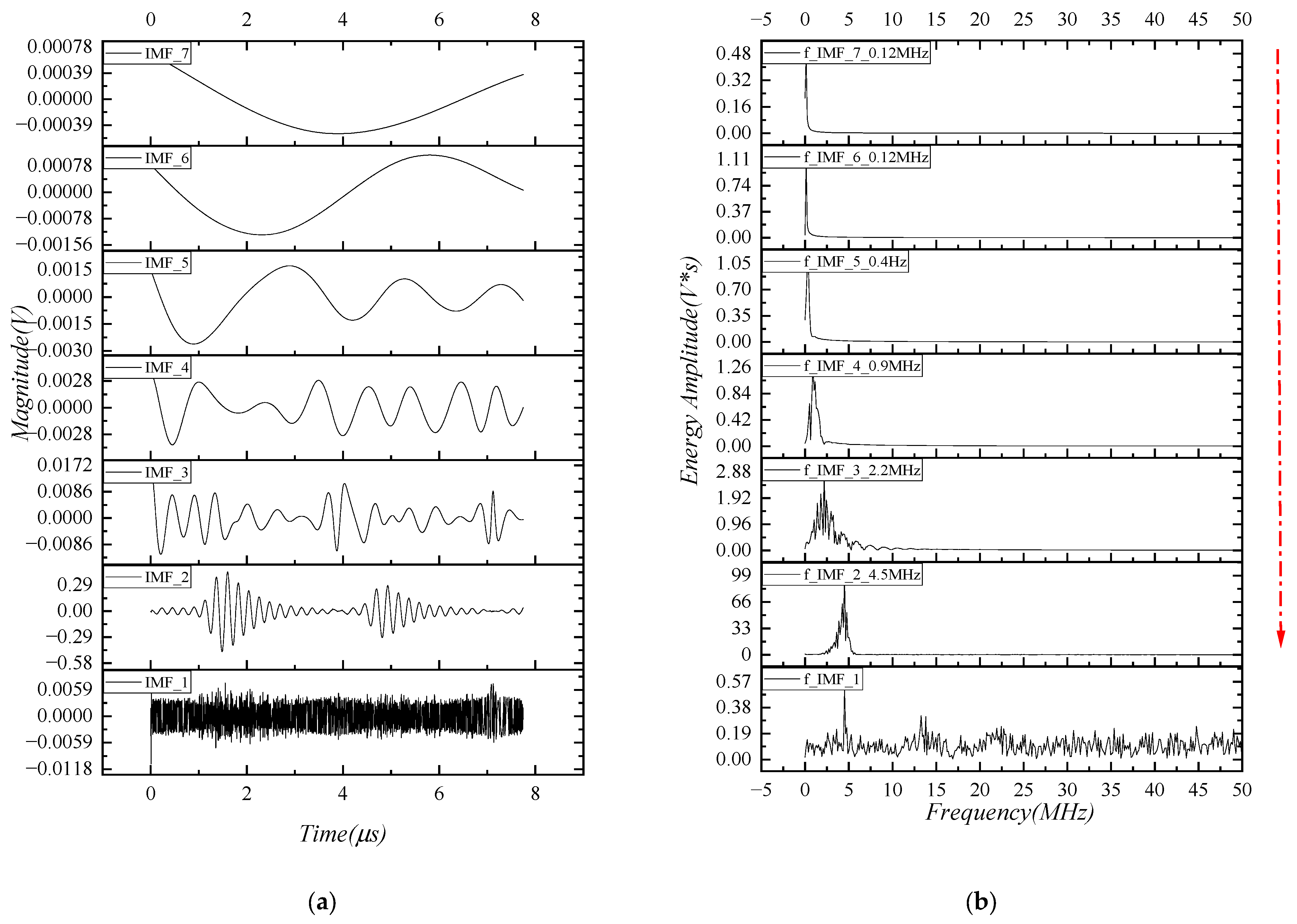
EMD analysis was applied to the ultrasonic echo signal in Figure 6 based on Equations (3) to (7). Figure 8a shows the IMF results of a representative ultrasonic echo signal extracted from 50 sets in the time domain. IMF2 to IMF6 satisfy the following two conditions: (1) The number of extreme points and the number of non-zero points are equal or differ by at most one, and (2) the average value of the upper envelope and the lower envelope is zero. The conditions are essential for the auto-diagnosis of ToF, as opposed to the manual adjusted recognition. IMF_7 represents the residual.
The appearance of IMF_2 looks the most similar to the original echo signal in Figure 8a, and the signal frequency of IMF_2 is close to the center frequency of the ultrasonic probe (5 MHz), which means that IMF_2 best suited for the subsequent signal processing. “Mode mixing” appeared in IMF_1, as shown in Figure 8a, due to signal interruption caused by a high-frequency oscillation at a certain point in the raw signal. Therefore, IMF_1 consisted of signals with many different frequencies as shown in Figure 8b, which cannot be devoted to signal processing. The sequences of Hilbert and EMD for signal processing are compared in Figure 9. With the Hilbert transform being performed first, the EMD results were not ideal due to the oscillation and discontinuity of the processed signal. A specific comparison of thickness estimation combined with the DPTM will be elaborated in Section 4.
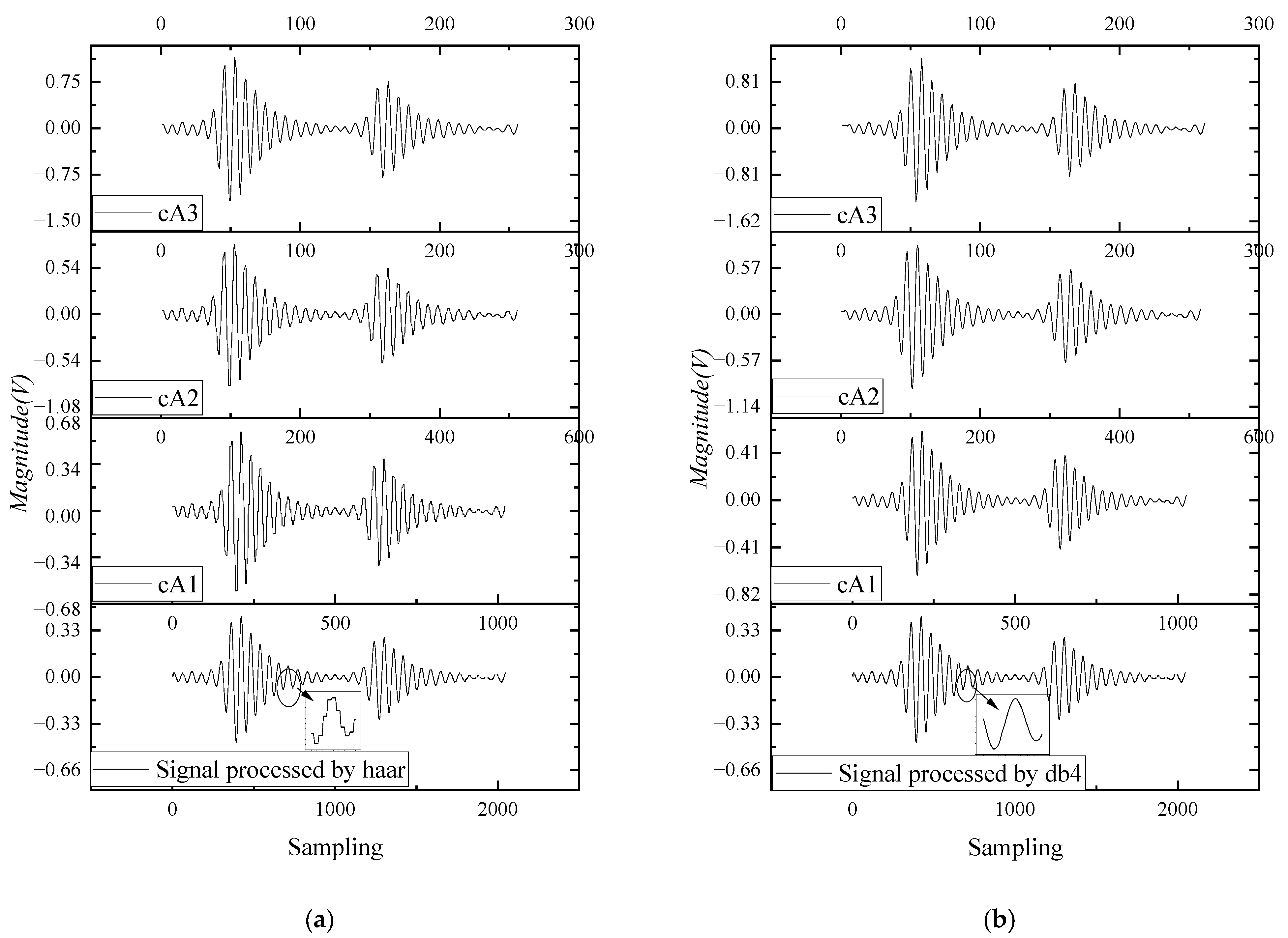
Difficulties in signal identification arose due to the superposition of noise and interference, while discontinuous oscillations in some high-frequency regions would result in “Mode mixing” during the EMD decomposition process as shown in Figure 8. The wavelet transform characterizes the features of the signal in both time and frequency domains, and obtains the corresponding effective information at low and high frequencies of the signal by adjusting the scale values. As the smoothness and accuracy of the signal reconstruction are preferred as the evaluation criterion in the selection process, haar and db4 were chosen as the wavelet bases for comparison and analysis.
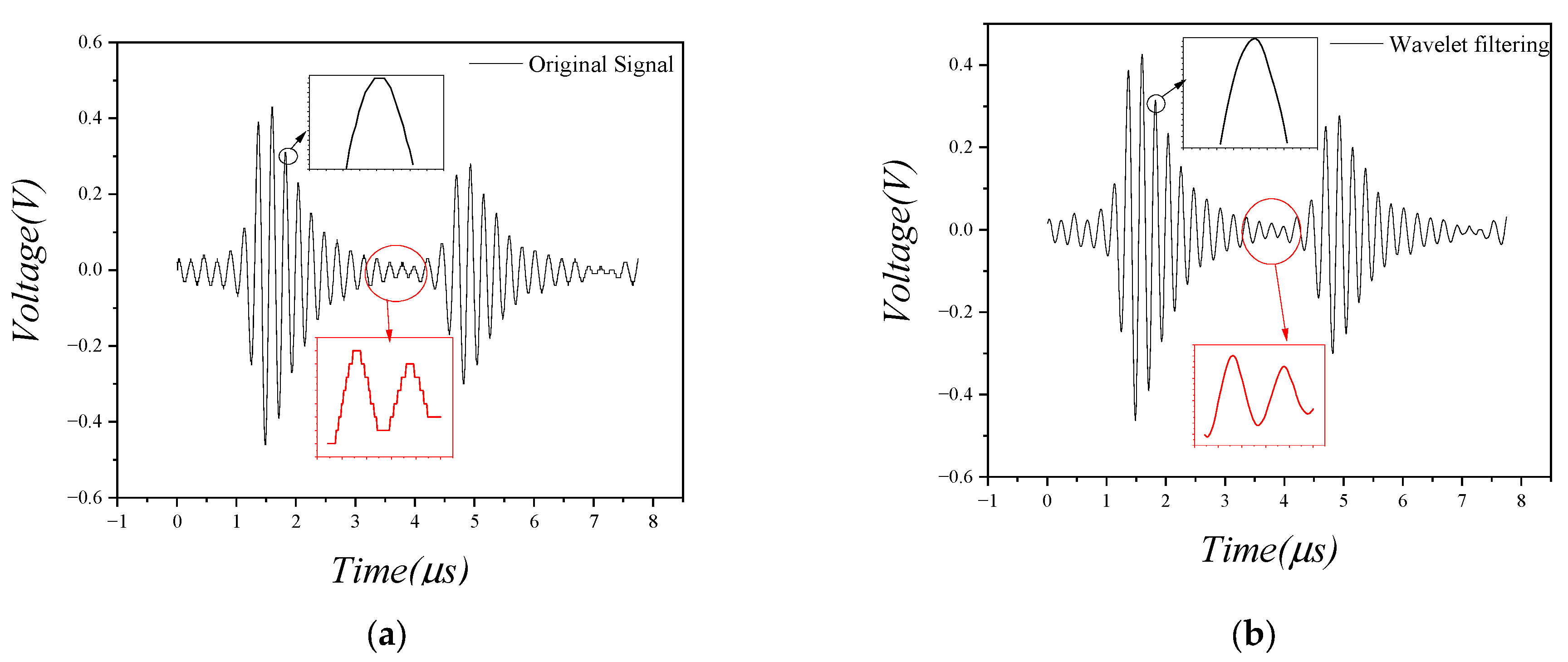
As shown in the insets of Figure 10, the signal processing with haar had fewer numbers of approximation coefficients of cA1(1023), cA2(512), and cA3(256) when compared to those of db4 (cA1(1026), cA2(516), and cA3(261)), which means that more complete information can be retained during the reconstructing process of the echo signal with db4. The oscillation of the signal got substantially less and the real information of the signal was retained after performing with db4 wavelet filtering as shown in Figure 11. The accuracy and smoothness of the signal could contribute to a much more accurate and faster estimation of the thickness in auto-diagnosis. Moreover, the method of selecting wavelet bases was adapted to specific requirements.
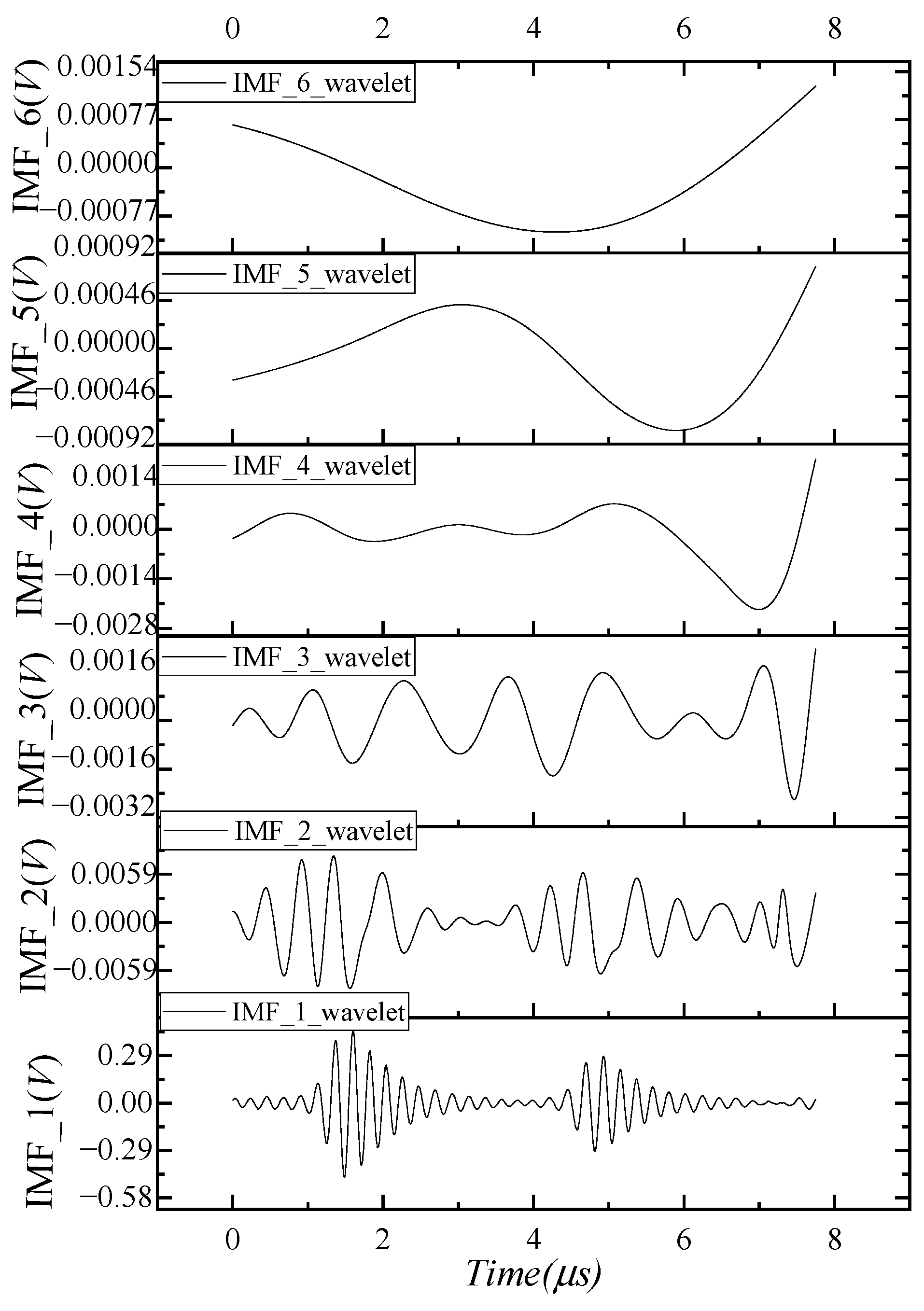
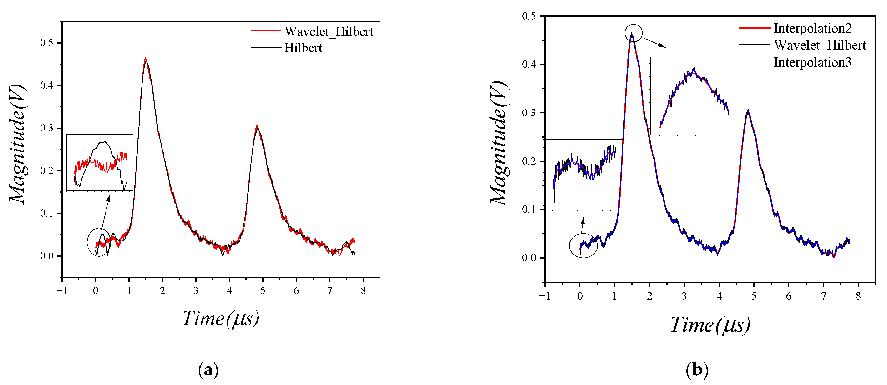
By performing EMD again after the wavelet transform as shown in Figure 12, the phenomenon of “Mode Mixing” was eliminated, the original information of the signal was preserved, and the noise was filtered out. Figure 13a shows that wavelet filtering could effectively reduce the amplitude of the oscillation after the Hilbert transformation. However, minor oscillations became apparent, which may increase the computational burden when there is a massive amount of data. A quadratic spline interpolation (interpolation 2) and a cubic spline interpolation (interpolation 3) in Section 3.3 were applied for smoothing the signal after wavelet filtering, respectively. After smoothing, the final envelope was good enough to perform an auto-diagnosis as shown in Figure 13b.
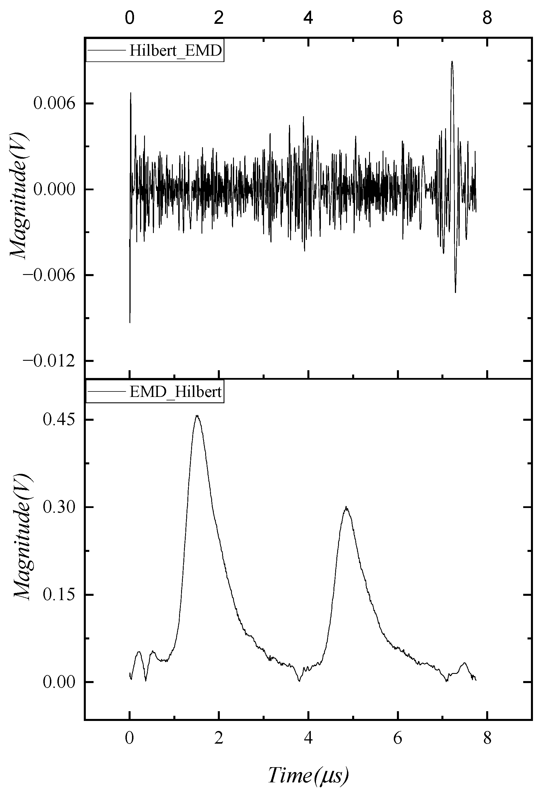
In Figure 14 and Table 1, ‘Hilbert_EMD’ (Approach 1) represents that the echo signal was firstly processed by Hilbert Transform; then, EMD analysis was used to decompose the echo signal into a different frequency. ‘EMD_Hilbert’ (Approach 2) represents that the echo signal was firstly processed by EMD analysis, and Hilbert Transform was then used to extract the echo signal with certain different frequencies. The DPTM model was eventually applied in the calculation of ToF. The difference between the two approaches lies in the order of the EMD analysis, in which the early stage of Hilbert transformation would cause signal distortion and oscillation on the estimation. ‘Hilbert_DPTM’ (Approach 3) represents that the signal was firstly filtered by wavelet and then subjected to Hilbert transform, and then, the DPTM was applied. ‘DPTM_Cross’ (Approach 4) represents that the signal was firstly processed by the DPTM and then subjected to the cross-correlation method. ‘Hilbert_DPTM_EMD’ (Approach 5) represents that the EMD analysis was performed after the wavelet filtering in ‘Hilbert_DPTM’. ‘DPTM_Interpolation2’ (Approach 6) and ‘DPTM_Interpolation3’ (Approach 7) represent that the echo signal was processed by a quadratic spline interpolation and a cubic spline interpolation, respectively, after the Wavelet, Hilbert, and DPTM. As shown in Table 1, the ‘DPTM_Cross’ and ‘DPTM_Interpolation2’ were the two most stable approaches.
To further investigate the potential of different algorithms for real application, a steel pipeline with a wall thickness of 7 mm was used as a testbed. Fifty sets of echo data were acquired in the pipeline under constant pressure at room temperature, as shown in Figure 15.
Through the comparison in Figure 16 and Table 2, the estimation accuracy of ‘DPTM_Interpolation2’ (Approach 6) was still the highest, and the standard deviation of the data was down to 0.01, indicating that the algorithm was very stable in the process of real-time estimation even for the actual pipeline.
To investigate the efficiency of the proposed approach for auto-diagnosis of ToF, various approaches in Table 2 were run 50 times through Matlab and the CPU times were recorded, respectively, as shown in Figure 17. According to the data analysis in Table 3, ‘DPTM_Cross’ (Approach 4) consumed the longest CPU time, while Hilbert_DPTM’ (Approach 3) ran the shortest time among the seven approaches. ‘Hilbert_EMD’ (Approach 1) and ‘EMD_Hilbert’ (Approach 2) consumed a similar amount of CPU time in which the sums of the CPU time were 12.73 s and 12.39 s, respectively. However, their standard deviations of the CPU time (0.13, and 0.16) were larger than those of ‘Hilbert_DPTM_EMD’ (Approach 5), ‘DPTM_Interpolation2’ (Approach 6) and ‘DPTM_Interpolation3’ (Approach 7) (0.06, 0.05, and 0.05). Among the approaches, ‘Hilbert_DPTM_EMD’ (Approach 5) and ‘DPTM_Interpolation2’ (Approach 6) showed the optimal efficiency, which had the same mean CPU time (0.26 s) while their standard deviation and sum of the CPU time were close.
5. Discussion
Based on the exploration of current ToF technology and signal processing in the field of UT, the DPTM-based auto-diagnosis was proposed and validated. Compared to the state-of-the-art approaches, the proposed intelligent inspection approach exhibits the following advantages:
- (1)
- No requirement for inputting the estimation range (e.g., thickness range) and detection location in advance, which is significant for achieving the intelligent application of ultrasonic NDT without the involvement of professional knowledge and specialized skills.
- (2)
- Great flexibility in the selection of the number of ultrasonic probes when compared with the strict requirements of conventional approaches for the equipment, e.g., the cross-correlation method requires the transceiver mode for real-time detection (at least a pair of ultrasonic transducers is required), which could greatly reduce the cost and complexity of detection.
- (3)
- Capable of achieving high accuracy on the thickness estimation for both 304SS plate and pipeline with defects, which could offer much more accurate defect localization and detection.
Nevertheless, the stability of the proposed algorithm still needs to improve, which could be affected by many external factors, such as the roughness of the testing object. Combining with other intelligent algorithms, such as a neural network, will be the focus of future work to resolve the issues induced by the roughness, the transducer frequency, the ambient temperature, and so on.
6. Conclusions
This article proposes a novel concept of realizing non-destructive detection intelligence. The algorithms for auto-diagnosis of ToF of ultrasonic signals have been investigated. To be capable of tracking and estimating ToF in real-time, the DPTM has also been proposed and applied to the ToF estimation for the first time. The experimental results show that the DPTM cannot only achieve the real-time estimation of ToF in the single-probe receiving mode in the time domain but also realize the single-probe receiving mode. The work is highly significant for the intelligent inspection of ultrasonic NDT.
As the actual testing conditions could be quite complicated, the DPTM may not be capable of encountering uncertainties without a “learning” function. In the future, the main work will focus on the excitation voltage to establish a neural network model to achieve a much more accurate and intelligent NDT. The target conditions such as pipeline roughness will also be added as the neural parameter for more intelligent defect identification on various testing targets. Neural networks for designing ultrasonic transducers will be further explored. There is still room for the development and application of neural networks in the field of ultrasonic NDT. The intelligent recognition of highly accurate and stable signals could be devoted to realizing unsupervised ultrasonic NDT with the advent of Industry 5.0.
Author Contributions
Conceptualization, F.Y. and D.S.; methodology, F.Y.; software, F.Y.; validation, F.Y., L.-y.L. and Q.M.; formal analysis, Q.M. and J.Z.; investigation, Q.M.; resources, F.Y.; data curation, F.Y. and L.-y.L.; writing—original draft preparation, F.Y. and Q.M.; writing—review and editing, K.-h.L.; visualization, F.Y.; supervision, K.-h.L.; project administration, K.-h.L.; funding acquisition, K.-h.L. All authors have read and agreed to the published version of the manuscript.
Funding
This research was funded by the Hong Kong Polytechnic University and University of Glasgow, funder: Kwok-ho Lam.
Data Availability Statement
The details about data supporting reported results can be found requested from the corresponding author.
Acknowledgments
Funding supported by the Hong Kong Polytechnic University and University of Glasgow.
Conflicts of Interest
All co-authors have seen and agreed with the content of the manuscript and there is no financial interest to report. We declare that the manuscript is original, which has not been published before or submitted elsewhere for consideration of publication. We know of no conflicts of interest associated with this work, and there has been no significant financial support for this work that could have influenced its outcome.
References
- Gupta, M.; Khan, M.A.; Butola, R.; Singari, R.M. Advances in applications of Non-Destructive Testing (NDT): A review. Adv. Mater. Process. Technol. 2021, 8, 2286–2307. [Google Scholar] [CrossRef]
- El Masri, Y.; Rakha, T. A scoping review of non-destructive testing (NDT) techniques in building performance diagnostic inspections. Constr. Build. Mater. 2020, 265, 120542. [Google Scholar] [CrossRef]
- Chauveau, D. Review of NDT and process monitoring techniques usable to produce high-quality parts by welding or additive manufacturing. Weld. World 2018, 62, 1097–1118. [Google Scholar] [CrossRef]
- Yang, Y.; Lu, H.; Tan, X.; Chai, H.K.; Wang, R.; Zhang, Y. Fundamental mode shape estimation and element stiffness evaluation of girder bridges by using passing tractor-trailers. Mech. Syst. Signal Process. 2021, 169, 108746. [Google Scholar] [CrossRef]
- Yang, Y.; Lu, H.; Tan, X.; Wang, R.; Zhang, Y. Mode Shape Identification and Damage Detection of Bridge by Movable Sensory System. IEEE Trans. Intell. Transp. Syst. 2022, PP, 1–15. [Google Scholar] [CrossRef]
- Yang, Y.; Ling, Y.; Tan, X.K.; Wang, S.; Wang, R.Q. Damage Identification of Frame Structure Based on Approximate Metropolis–Hastings Algorithm and Probability Density Evolution Method. Int. J. Struct. Stab. Dyn. 2022, 22. [Google Scholar] [CrossRef]
- Pyle, R.J.; Bevan, R.L.T.; Hughes, R.R.; Rachev, R.K.; Ali, A.A.S.; Wilcox, P.D. Deep Learning for Ultrasonic Crack Characterization in NDE. IEEE Trans. Ultrason. Ferroelectr. Freq. Control 2021, 68, 1854–1865. [Google Scholar] [CrossRef]
- Dong, Z.; Mai, Z.; Yin, S.; Wang, J.; Yuan, J.; Fei, Y. A weld line detection robot based on structure light for automatic NDT. Int. J. Adv. Manuf. Technol. 2020, 111, 1831–1845. [Google Scholar] [CrossRef]
- Jolly, M.R.; Prabhakar, A.; Sturzu, B.; Hollstein, K.; Singh, R.; Thomas, S.; Foote, P.; Shaw, A. Review of non-destructive testing (NDT) techniques and their applicability to thick walled composites. Procedia CIRP 2015, 38, 129–136. [Google Scholar] [CrossRef] [Green Version]
- Li-ying, S.; Xiao-dong, Y.; Yi-bo, L. Research on transducer and frequency of ultrasonic guided waves in urban pipe inspection. In Proceedings of the 2009 4th IEEE Conference on Industrial Electronics and Applications, Xi’an, China, 25–27 May 2009. [Google Scholar]
- Zeng, W.; Yao, Y.J.O. Numerical simulation of laser-generated ultrasonic waves for detection surface defect on a cylinder pipe. Optik 2020, 212, 164650. [Google Scholar] [CrossRef]
- Yu, Y.; Safari, A.; Niu, X.; Drinkwater, B.; Horoshenkov, K.V. Acoustic and ultrasonic techniques for defect detection and condition monitoring in water and sewerage pipes: A review. Appl. Acoust. 2021, 183, 108282. [Google Scholar] [CrossRef]
- Zheng, G.; Tian, Y.; Zhao, W.; Jia, S.; Peng, S. Realization and application of an improved multi-fold method for ultrasonic guided wave. Structures 2022, 38, 1607–1614. [Google Scholar] [CrossRef]
- Khalili, P.; Cawley, P. The choice of ultrasonic inspection method for the detection of corrosion at inaccessible locations. NDT E Int. 2018, 99, 80–92. [Google Scholar] [CrossRef]
- Ahmad, A.; Bond, L.J.; Glass, I.S.W.; Lindgren, E.; Forsyth, D.; Aldrin, J.; Spencer, F.; Schafbuch, P.; Antonatos, A.; Radkowski, R.; et al. Fundamentals of Ultrasonic Inspection; Springer: New York, NY, USA, 2018; Volume 17, pp. 155–168. [Google Scholar]
- Schmerr, L.W. Fundamentals of Ultrasonic Nondestructive Evaluation; Springer: New York, NY, USA, 2016; Volume 122. [Google Scholar]
- Comminiello, D.; Scarpiniti, M.; Parisi, R.; Uncini, A. Frequency-domain adaptive filtering: From real to hypercomplex signal processing. In Proceedings of the ICASSP 2019—2019 IEEE International Conference on Acoustics, Speech and Signal Processing (ICASSP), Brighton, UK, 12–17 May 2019. [Google Scholar]
- Wei, P.; Dan, L.; Xiao, Y.; Li, S. A low-complexity time-domain signal processing algorithm for N-continuous OFDM. In Proceedings of the 2013 IEEE International Conference on Communications (ICC), Budapest, Hungary, 9–13 June 2013. [Google Scholar]
- Aoki, K.; Suga, Y. Application of artificial neural network to discrimination of defect type in automatic radiographic testing of welds. ISIJ Int. 1999, 39, 1081–1087. [Google Scholar] [CrossRef]
- Valle, M.; Onorato, M.; Oddone, F.; Caviglia, D.; Bisio, G. An analog VLSI neural network for real-time image processing in industrial applications. In Proceedings of the Seventh Annual IEEE International ASIC Conference and Exhibit, Rochester, NY, USA, 19–23 September 1994. [Google Scholar]
- Gleich, B.; Weizenecker, J. Tomographic imaging using the nonlinear response of magnetic particles. Nature 2005, 435, 1214–1217. [Google Scholar] [CrossRef]
- Rahmer, J.; Weizenecker, J.; Gleich, B.; Borgert, J. Signal encoding in magnetic particle imaging: Properties of the system function. BMC Med. Imaging 2009, 9, 4. [Google Scholar] [CrossRef] [Green Version]
- Grüttner, M.; Knopp, T.; Franke, J.; Heidenreich, M.; Rahmer, J.; Halkola, A.; Kaethner, C.; Borgert, J.; Buzug, T.M. On the formulation of the image reconstruction problem in magnetic particle imaging. Biomed. Tech. 2013, 58, 583–591. [Google Scholar] [CrossRef]
- Ilbey, S.; Top, C.B.; Güngör, A.; Çukur, T.; Sarıtaş, E.Ü.; Güven, H.E. Comparison of system-matrix-based and projection-based reconstructions for field free line magnetic particle imaging. Int. J. Magn. Part. Imaging 2017, 3, 1–8. [Google Scholar]
- Kaethner, C.; Erb, W.; Ahlborg, M.; Szwargulski, P.; Knopp, T.; Buzug, T.M. Non-equispaced system matrix acquisition for magnetic particle imaging based on Lissajous node points. IEEE Trans. Med. Imaging 2016, 35, 2476–2485. [Google Scholar] [CrossRef]
- Panagiotopoulos, N.; Vogt, F.; Barkhausen, J.; Buzug, T.M.; Duschka, R.L.; Lüdtke-Buzug, K.; Ahlborg, M.; Bringout, G.; Debbeler, C.; Gräser, M.; et al. Magnetic particle imaging: Current developments and future directions. Int. J. Nanomed. 2015, 10, 3097. [Google Scholar] [CrossRef] [Green Version]
- Migoun, N.; Delenkovskii, N.V. Improvement of penetrant-testing methods. Eng. Phys. Thermophys. 2009, 82, 734–742. [Google Scholar] [CrossRef]
- Sun, X.; Man, J.; Chen, D.; Fei, C.; Li, D.; Zhu, Y.; Zhao, T.; Feng, W.; Yang, Y. Intelligent optimization of matching layers for piezoelectric ultrasonic transducer. IEEE Sens. J. 2021, 21, 13107–13115. [Google Scholar] [CrossRef]
- Zhou, Q.; Lam, K.H.; Zheng, H.; Qiu, W.; Shung, K.K. Piezoelectric single crystal ultrasonic transducers for biomedical applications. Prog. Mater. Sci. 2014, 66, 87–111. [Google Scholar] [CrossRef] [PubMed] [Green Version]
- Chen, D.; Hou, C.; Fei, C.; Li, D.; Lin, P.; Chen, J.; Yang, Y. An optimization design strategy of 1–3 piezocomposite ultrasonic transducer for imaging applications. Mater. Today Commun. 2020, 24, 100991. [Google Scholar] [CrossRef]
- Sambath, S.; Nagaraj, P.; Selvakumar, N. Automatic defect classification in ultrasonic NDT using artificial intelligence. Nondestruct. Eval. 2011, 30, 20–28. [Google Scholar] [CrossRef]
- Fradkin, L.; Altinbasak, S.U.; Darmon, M. Towards Explainable Augmented Intelligence (AI) for Crack Characterization. Appl. Sci. 2021, 11, 10867. [Google Scholar] [CrossRef]
- Feng, B.; Pasadas, D.J.; Ribeiro, A.L.; Ramos, H.G. Locating Defects in Anisotropic CFRP Plates Using ToF-Based Probability Matrix and Neural Networks. IEEE Trans. Instrum. Meas. 2019, 68, 1252–1260. [Google Scholar] [CrossRef]
- Shi, Y.; Xu, W.; Zhang, J.; Li, X. Automated Classification of Ultrasonic Signal via a Convolutional Neural Network. Appl. Sci. 2022, 12, 4179. [Google Scholar] [CrossRef]
- Park, S.-H.; Choi, S.; Jhang, K.-Y. Porosity evaluation of additively manufactured components using deep learning-based ultrasonic nondestructive testing. Int. J. Precis. Eng. Manuf. Technol. 2022, 9, 395–407. [Google Scholar] [CrossRef]
- Diogo, A.R.; Moreira, B.; Gouveia, C.A.J.; Tavares, J.M.R.S. A Review of Signal Processing Techniques for Ultrasonic Guided Wave Testing. Metals 2022, 12, 936. [Google Scholar] [CrossRef]
- Kononenko, I. Bayesian neural networks. Biol. Cybern. 1989, 61, 361–370. [Google Scholar] [CrossRef]
- Harley, J.B.; Sparkman, D. Machine learning and NDE: Past, present, and future. AIP Conf. Proc. 2019, 2102, 090001. [Google Scholar]
- Ma, J.; Xu, K.-J.; Jiang, Z.; Zhang, L.; Xu, H.-R. Applications of digital signal processing methods in TOF calculation of ultrasonic gas flowmeter. Flow Meas. Instrum. 2021, 79, 101932. [Google Scholar] [CrossRef]
- Juan, C.W.; Hu, J.S. Single-object localization using multiple ultrasonic sensors and constrained weighted least-squares method. Asian J. Control. 2021, 23, 1171–1184. [Google Scholar] [CrossRef]
- Malikov, A.K.; Cho, Y.; Kim, Y.H.; Kim, J.; Park, J.; Yi, J.H. Ultrasonic assessment of thickness and bonding quality of coating layer based on short-time fourier transform and convolutional neural networks. Coatings 2021, 11, 909. [Google Scholar] [CrossRef]
- Song, Q.; Ma, X. High-resolution time delay estimation algorithms through cross-correlation post-processing. IEEE Signal Process. Lett. 2021, 28, 479–483. [Google Scholar] [CrossRef]
- Sharkova, S.; Faerman, V.A. Wavelet transform-based cross-correlation in the time-delay estimation applications. J. Phys. Conf. Ser. 2021, 2142, 012019. [Google Scholar] [CrossRef]
- Faerman, V.; Sharkova, S.; Avramchuk, V.; Shkunenko, V. Towards applicability of wavelet-based cross-correlation in locating leaks in steel water supply pipes. J. Phys. Conf. Ser. 2022, 2176, 012067. [Google Scholar] [CrossRef]
- Li, W.; Chen, Q.; Wu, J. Double threshold ultrasonic distance measurement technique and its application. Rev. Sci. Instrum. 2014, 85, 044905. [Google Scholar] [CrossRef]
- Huang, P.; Yang, Y.; Huang, T. Real-time measurement of model attitude based on NDT and ICP. In Proceedings of the 4th Optics Young Scientist Summit (OYSS 2020), Ningbo, China, 4–7 December 2020. [Google Scholar]
- Zheng, D.; Mao, Y.; Yang, Z. A new characteristic peaks group judgement method for the accurate measurement of time-of-flight in the ultrasonic gas flowmeter. IET Sci. Meas. Technol. 2021, 15, 597–605. [Google Scholar] [CrossRef]
- Zheng, D.; Mei, J.; Mao, Y.; Yang, Z. Signal processing method for flight time measurement of gas ultrasonic flowmeter. In Proceedings of the 2021 IEEE International Instrumentation and Measurement Technology Conference (I2MTC), Glasgow, UK, 17–20 May 2021. [Google Scholar]
- Juan, C.-W.; Hu, J.-S. Object Localization and Tracking System Using Multiple Ultrasonic Sensors with Newton–Raphson Optimization and Kalman Filtering Techniques. Appl. Sci. 2021, 11, 11243. [Google Scholar] [CrossRef]
- Thangarajoo, R.G.; Reaz, M.B.I.; Srivastava, G.; Haque, F.; Ali, S.H.M.; Bakar, A.A.A.; Bhuiyan, M.A.S. Machine learning-based epileptic seizure detection methods using wavelet and EMD-based decomposition techniques: A review. Sensors 2021, 21, 8485. [Google Scholar] [CrossRef] [PubMed]
Figure 1.
Isotropic cross-section view of the transducer fixture.

Figure 2.
Ultrasound detection setup for raw data collection.

Figure 3.
ToF evaluation process and application(Violet line represents the signal envelope; Colorful lines represents echo signal).
Figure 3.
ToF evaluation process and application(Violet line represents the signal envelope; Colorful lines represents echo signal).

Figure 4.
Flowchart of DPTM process.

Figure 5.
Adaptive defects inspection method diagram.

Figure 6.
50 sets of data on a steel plate under constant pressure.

Figure 7.
Statistics of ultrasonic echo signals in Figure 6.
Figure 7.
Statistics of ultrasonic echo signals in Figure 6.

Figure 8.
(a) IMF results of a representative ultrasonic echo signal acquired with a 304SS sample, and (b) the corresponding frequency spectra(Frequency increases as the red line).
Figure 8.
(a) IMF results of a representative ultrasonic echo signal acquired with a 304SS sample, and (b) the corresponding frequency spectra(Frequency increases as the red line).

Figure 9.
Comparison sequences of Hilbert_EMD and EMD_Hilbert for signal processing.

Figure 10.
Signals processed with wavelet approximation coefficients for (a) db4 wavelet base and (b) haar wavelet base.
Figure 10.
Signals processed with wavelet approximation coefficients for (a) db4 wavelet base and (b) haar wavelet base.

Figure 11.
(a) Original ultrasonic echo signal, and (b) the signal after wavelet filtering.

Figure 12.
IMF results of a representative ultrasonic echo signal acquired with a 304SS sample from low to high frequencies after wavelet filtering.
Figure 12.
IMF results of a representative ultrasonic echo signal acquired with a 304SS sample from low to high frequencies after wavelet filtering.

Figure 13.
Comparison of signals (a) before and after wavelet filtering, and (b) before and after interpolation.
Figure 13.
Comparison of signals (a) before and after wavelet filtering, and (b) before and after interpolation.

Figure 14.
Results acquired on a 304SS plate using different approaches listed in Table 1.
Figure 14.
Results acquired on a 304SS plate using different approaches listed in Table 1.

Figure 15.
(a) 50 sets of data on a steel plate under constant pressure, and (b) a photo of a steel pipeline with a wall thickness of 7 mm for verifying the DPTM.
Figure 15.
(a) 50 sets of data on a steel plate under constant pressure, and (b) a photo of a steel pipeline with a wall thickness of 7 mm for verifying the DPTM.

Figure 16.
Results acquired in a pipeline obtained using different approaches.

Figure 17.
Comparison of CPU times by Matlab using different approaches.


Table 1.
Comparison of results acquired on a steel plate using different approaches.
| Approach | Mean (mm) | Standard Deviation | Sum (mm) | Minimum (mm) | Median (mm) | Maximum (mm) | Maximum Auto-Diagnosis Error | |
|---|---|---|---|---|---|---|---|---|
| 1 | Hilbert_EMD | 9.84 | 0.94 | 492.41 | 3.90 | 9.950 | 12.59 | 60.93% |
| 2 | EMD_Hilbert | 9.95 | 0.19 | 497.74 | 9.49 | 9.963 | 10.76 | 0.49% |
| 3 | Hilbert_DPTM | 9.96 | 0.00 | 498.16 | 9.96 | 9.963 | 9.96 | 0.37% |
| 4 | DPTM_Cross | 9.95 | 0.00 | 497.60 | 9.95 | 9.952 | 9.95 | 0.48% |
| 5 | Hilbert_DPTM_EMD | 9.95 | 0.01 | 497.56 | 9.87 | 9.952 | 9.96 | 1.27% |
| 6 | DPTM_Interpolation2 | 9.97 | 0.00 | 498.73 | 9.97 | 9.975 | 9.97 | 0.25% |
| 7 | DPTM_Interpolation3 | 9.96 | 0.10 | 498.35 | 9.96 | 9.963 | 9.97 | 0.37% |
Table 2.
Comparisons of results in a pipeline obtained using different approaches.
| Approach | Mean (mm) | Standard Deviation | Sum (mm) | Minimum (mm) | Median (mm) | Maximum (mm) | Maximum Auto-Diagnosis Error | |
|---|---|---|---|---|---|---|---|---|
| 1 | Hilbert_EMD | 7.16 | 3.85 | 358.48 | 2.34 | 6.58 | 21.64 | 209.25% |
| 2 | EMD_ Hilbert | 8.99 | 7.61 | 449.76 | 0.03 | 7.46 | 23.04 | 229.15% |
| 3 | Hilbert_DPTM | 2.70 | 2.06 | 132.33 | 0.97 | 1.36 | 6.79 | 86.14% |
| 4 | DPTM_Cross | 7.16 | 0 | 358.34 | 7.16 | 7.16 | 7.16 | 2.38% |
| 5 | Hilbert_DPTM_EMD | 10.63 | 6.32 | 531.66 | 0.71 | 7.78 | 21.55 | 207.86% |
| 6 | DPTM_Interpolation2 | 6.93 | 0.01 | 346.88 | 6.91 | 6.94 | 6.96 | 1.25% |
| 7 | DPTM_Interpolation3 | 6.45 | 0.91 | 322.91 | 1.51 | 6.79 | 7.15 | 78.32% |
Table 3.
Comparison of CPU times by Matlab using different approaches.
| Approach | Mean (s) | Standard Deviation | Sum (s) | Minimum (s) | Median (s) | Maximum (s) | |
|---|---|---|---|---|---|---|---|
| 1 | Hilbert_EMD | 0.25 | 0.13 | 12.73 | 0.12 | 0.21 | 0.92 |
| 2 | EMD_ Hilbert | 0.24 | 0.10 | 12.39 | 0.14 | 0.22 | 0.71 |
| 3 | Hilbert_DPTM | 0.22 | 0.04 | 11.03 | 0.14 | 0.20 | 0.32 |
| 4 | DPTM_Cross | 1.46 | 0.21 | 73.48 | 0.87 | 1.46 | 2.09 |
| 5 | Hilbert_DPTM_EMD | 0.26 | 0.06 | 13.40 | 0.15 | 0.26 | 0.42 |
| 6 | DPTM_Interpolation2 | 0.26 | 0.05 | 13.23 | 0.17 | 0.26 | 0.40 |
| 7 | DPTM_Interpolation3 | 0.29 | 0.05 | 14.51 | 0.17 | 0.29 | 0.39 |
Disclaimer/Publisher’s Note: The statements, opinions and data contained in all publications are solely those of the individual author(s) and contributor(s) and not of MDPI and/or the editor(s). MDPI and/or the editor(s) disclaim responsibility for any injury to people or property resulting from any ideas, methods, instructions or products referred to in the content. |
© 2023 by the authors. Licensee MDPI, Basel, Switzerland. This article is an open access article distributed under the terms and conditions of the Creative Commons Attribution (CC BY) license (https://creativecommons.org/licenses/by/4.0/).
Share and Cite
MDPI and ACS Style
Yang, F.; Shi, D.; Lo, L.-Y.; Mao, Q.; Zhang, J.; Lam, K.-H. Auto-Diagnosis of Time-of-Flight for Ultrasonic Signal Based on Defect Peaks Tracking Model. Remote Sens. 2023, 15, 599. https://doi.org/10.3390/rs15030599
AMA Style
Yang F, Shi D, Lo L-Y, Mao Q, Zhang J, Lam K-H. Auto-Diagnosis of Time-of-Flight for Ultrasonic Signal Based on Defect Peaks Tracking Model. Remote Sensing. 2023; 15(3):599. https://doi.org/10.3390/rs15030599
Chicago/Turabian StyleYang, Fan, Dongliang Shi, Long-Yin Lo, Qian Mao, Jiaming Zhang, and Kwok-Ho Lam. 2023. "Auto-Diagnosis of Time-of-Flight for Ultrasonic Signal Based on Defect Peaks Tracking Model" Remote Sensing 15, no. 3: 599. https://doi.org/10.3390/rs15030599
Note that from the first issue of 2016, this journal uses article numbers instead of page numbers. See further details here.