
Comparison of Three Different Random Forest Approaches to Retrieve Daily High-Resolution Snow Cover Maps from MODIS and Sentinel-2 in a Mountain Area, Gran Paradiso National Park (NW Alps)

Abstract
:1. Introduction
2. Materials and Methods
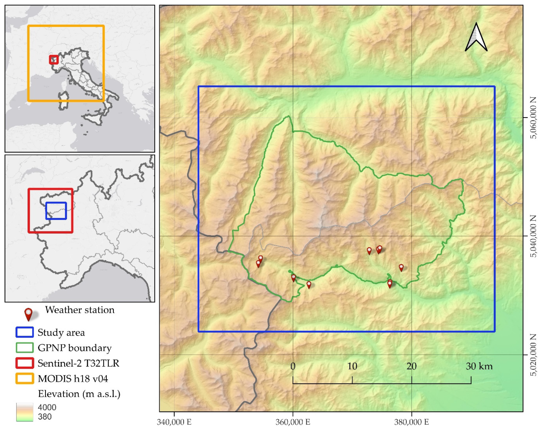
2.1. Study Area
2.2. Data
2.2.1. MODIS
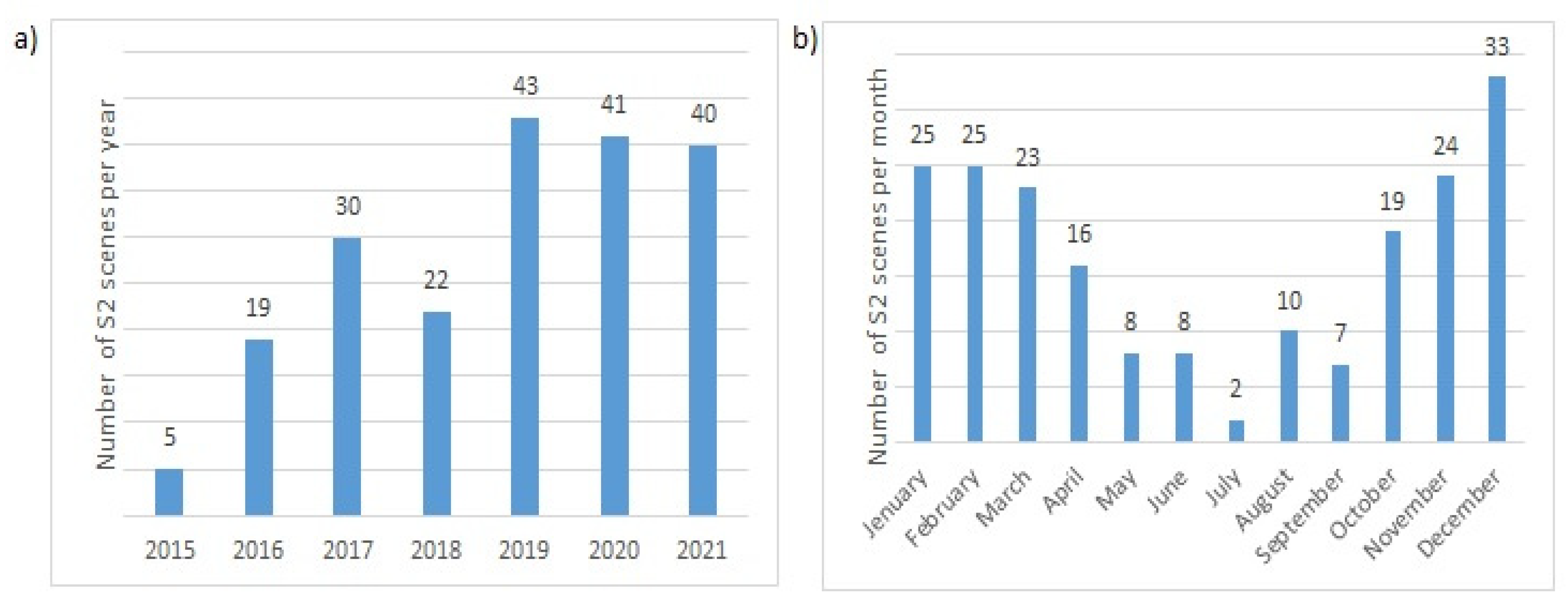
2.2.2. Sentinel-2
2.2.3. Digital Elevation Model
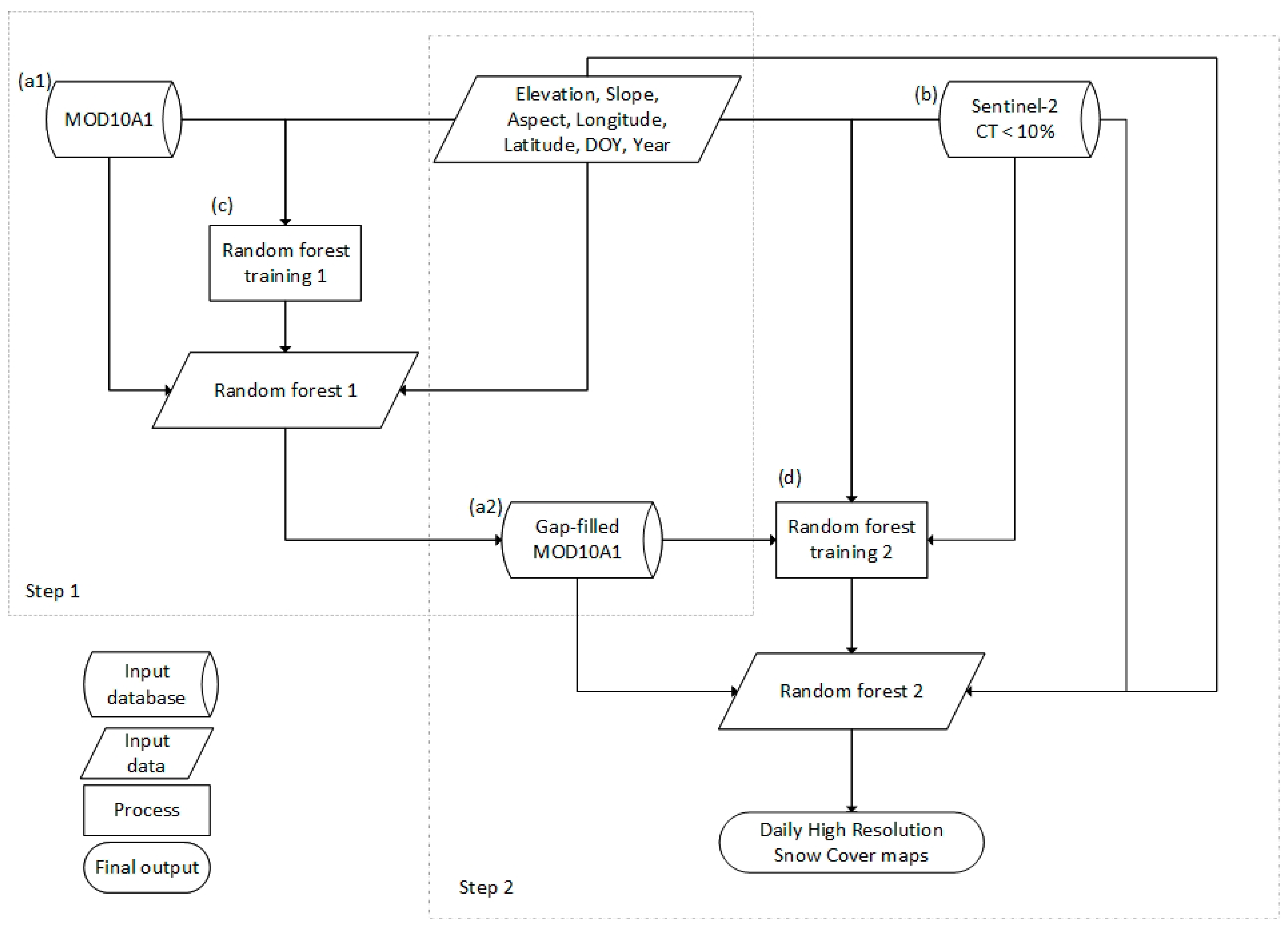
2.3. Workflow: Two-Stage Random Forests
- The first approach (A1) uses the FSC data from MODIS as input for a regression RF in the first step, along with the binary Snow Cover Extent (SCE) product from S2 for a classification RF in the second step.
- The second approach (A2) uses the MODIS FSC as input for a regression RF in the first step, and the Normalized Difference Snow Index (NDSI) from S2 for the second step.
- The third approach (A3) uses the raw NDSI maps from both MODIS and S2 and a regression RF in both the first and second steps, respectively.
Random Forest
- ntree: Number of trees grown by the forest;
- mtry: Number of variables randomly sampled as candidates at each split;
- node size: Minimum number of observations in a terminal node.
2.4. Validation
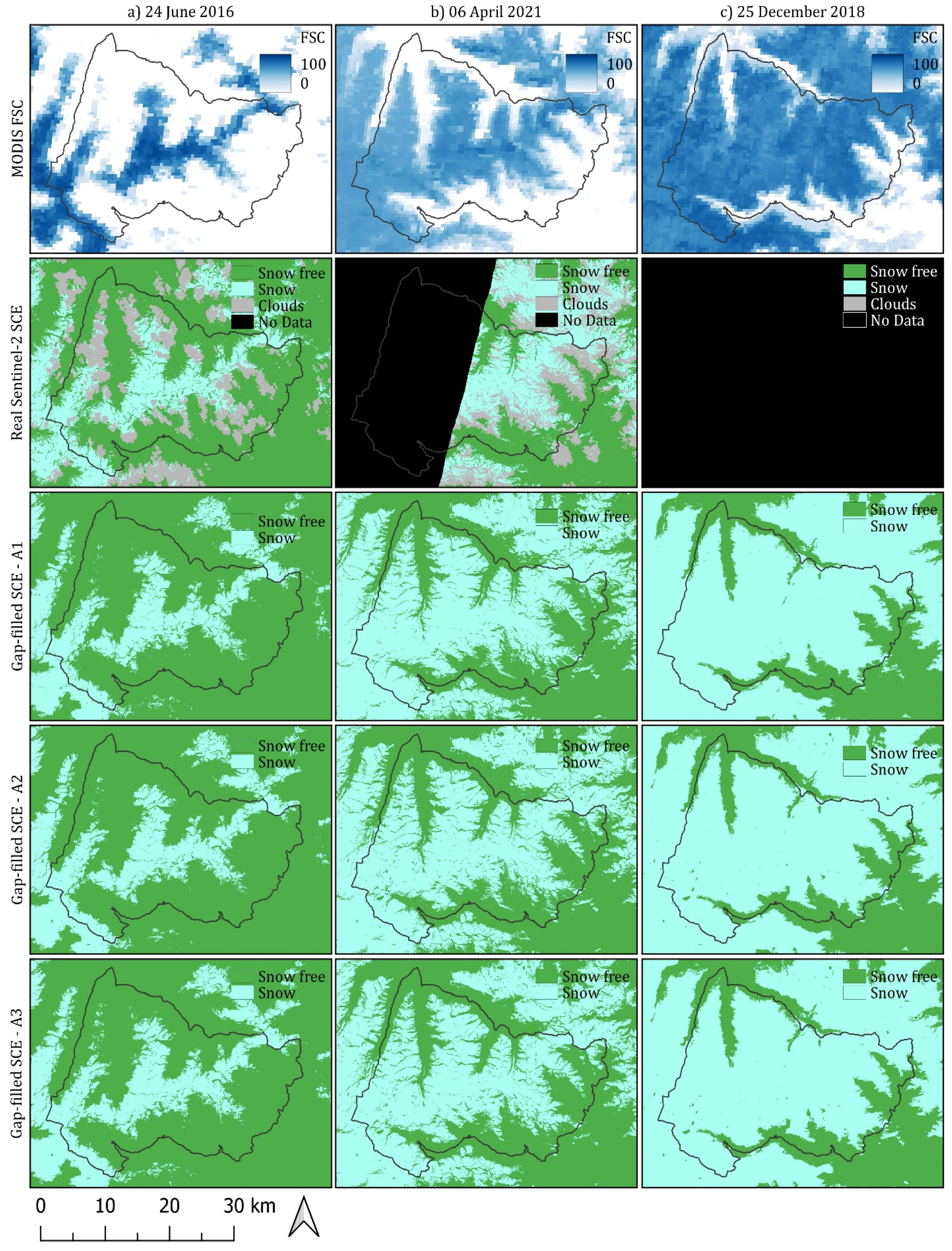
2.4.1. Comparison with Real Sentinel-2 SCE Maps
2.4.2. Comparison with In Situ Measurements from Weather Stations
2.4.3. Evaluation Metrics
3. Results
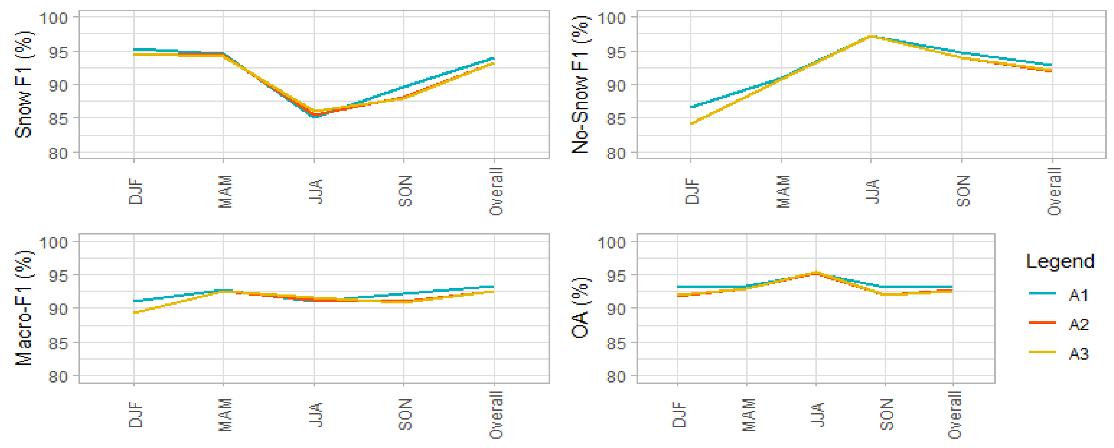
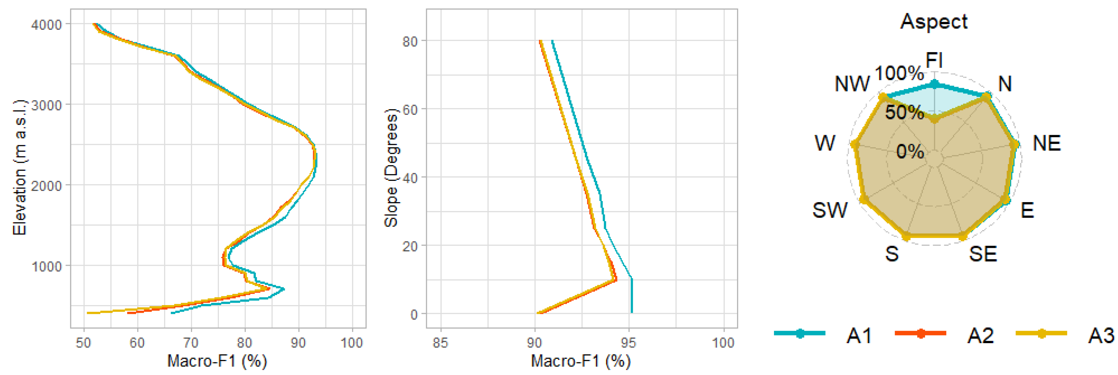
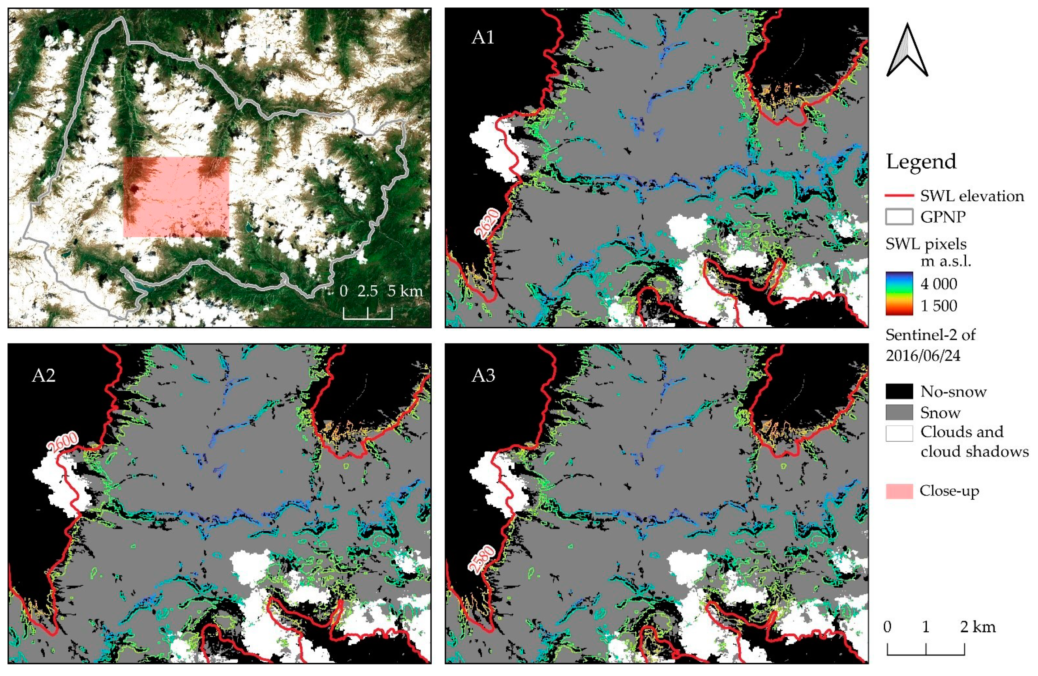
3.1. Comparison with Real Sentinel-2 SCE Maps
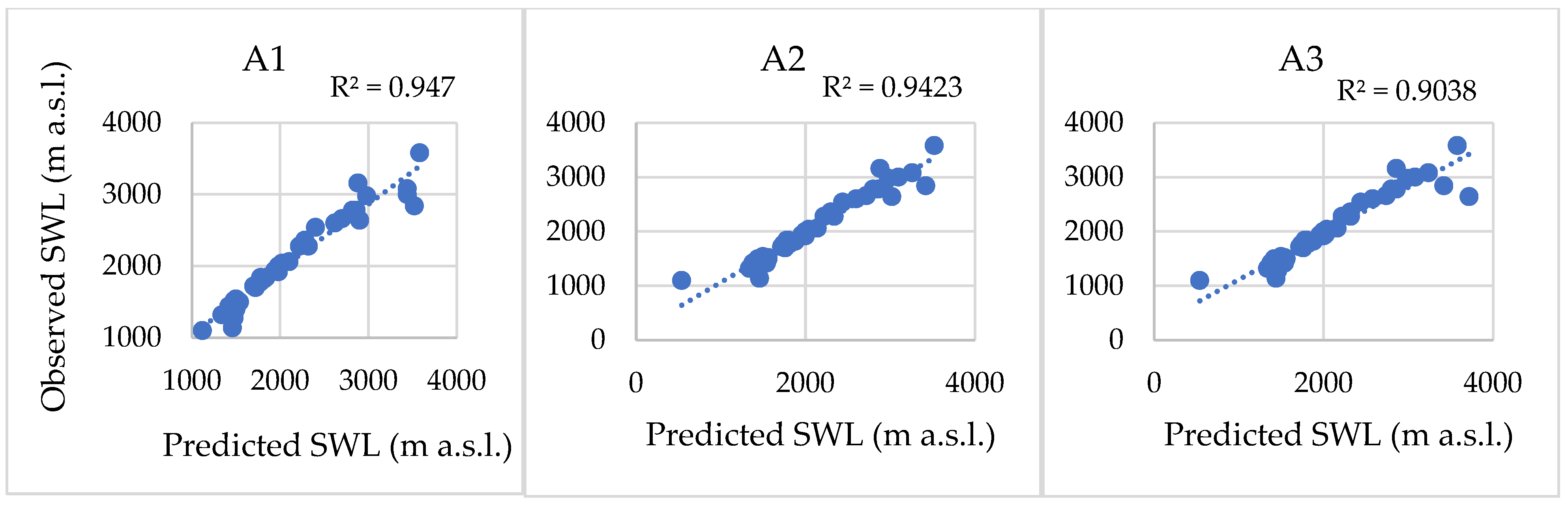
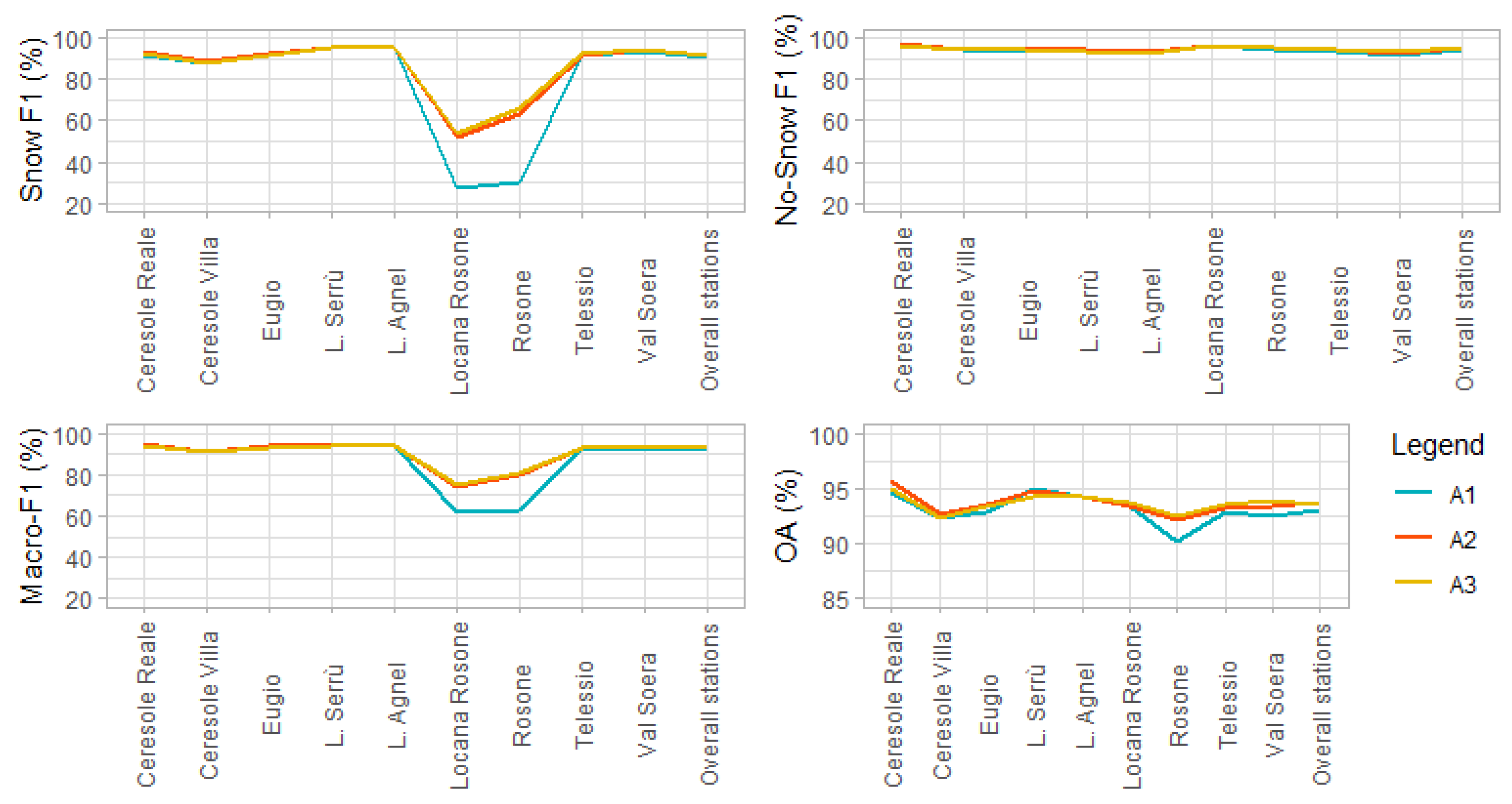
3.2. Comparison with In Situ Measurements from Weather Stations
3.3. McNemar Test
3.4. Random Forests
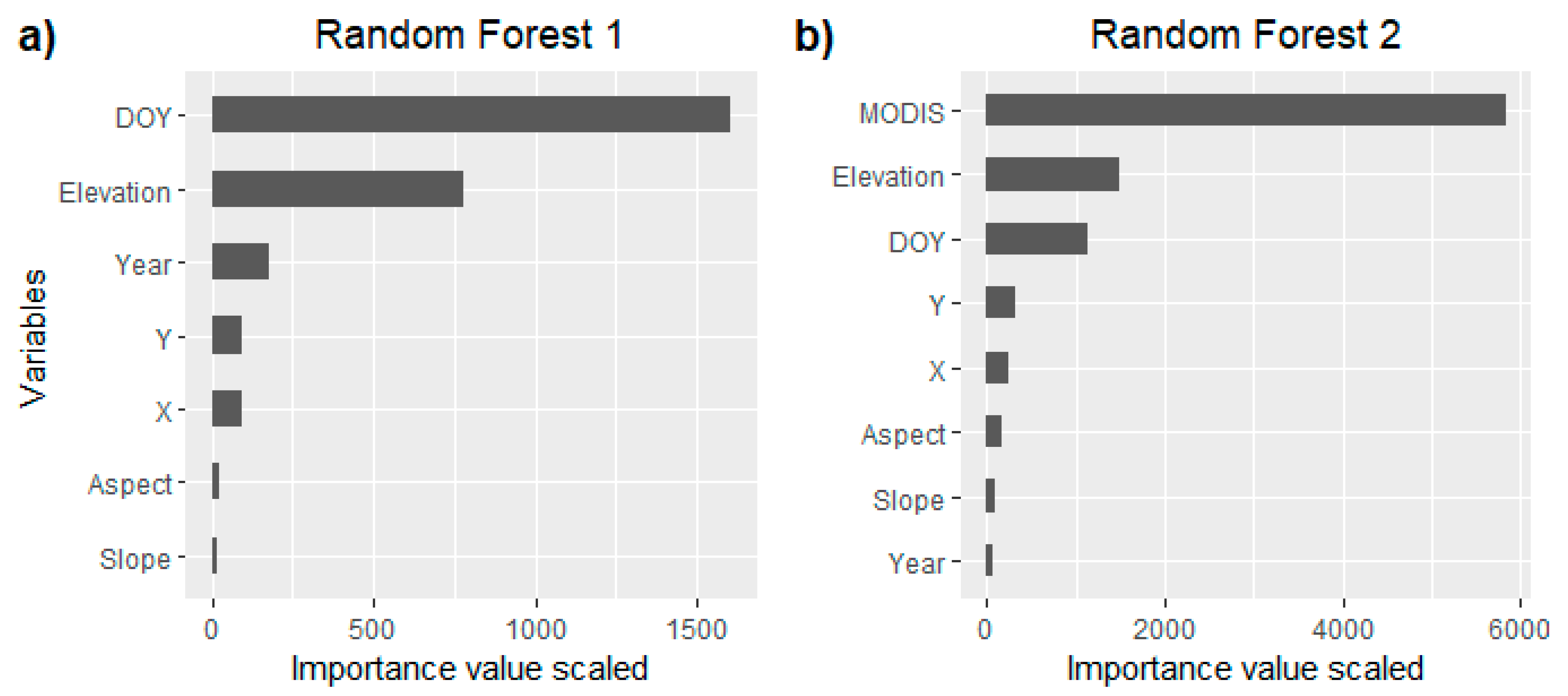
Variable Importance
4. Discussion
5. Conclusions
Supplementary Materials
Author Contributions
Funding
Data Availability Statement
Acknowledgments
Conflicts of Interest
References
- Zhang, T. Influence of the seasonal snow cover on the ground thermal regime: An overview. Rev. Geophys. 2005, 43, 4002. [Google Scholar] [CrossRef]
- Zhu, J.; Wu, Q.; Wu, F.; Yue, K.; Ni, X. Decline in carbon decomposition from litter after snow removal is driven by a delayed release of carbohydrates. Plant Soil 2022, 7, 1–13. [Google Scholar] [CrossRef]
- Bormann, K.J.; Brown, R.D.; Derksen, C.; Painter, T.H. Estimating snow-cover trends from space. Nat. Clim. Chang. 2018, 8, 924–928. [Google Scholar] [CrossRef]
- Rixen, C.; Høye, T.T.; Macek, P.; Aerts, R.; Alatalo, J.M.; Anderson, J.T.; Arnold, P.A.; Barrio, I.C.; Bjerke, J.W.; Björkman, M.P.; et al. Winters are changing: Snow effects on Arctic and alpine tundra ecosystems. Arct. Sci. 2022, 8, 572–608. [Google Scholar] [CrossRef]
- Rumpf, S.B.; Gravey, M.; Brönnimann, O.; Luoto, M.; Cianfrani, C.; Mariethoz, G.; Guisan, A. From white to green: Snow cover loss and increased vegetation productivity in the European Alps. Science 2022, 376, 1119–1122. [Google Scholar] [CrossRef] [PubMed]
- Yang, Y.; Wu, X.-J.; Liu, S.-W.; Xiao, C.-D.; Wang, X. Valuating service loss of snow cover in Irtysh River Basin. Adv. Clim. Chang. Res. 2019, 10, 109–114. [Google Scholar] [CrossRef]
- Wu, X.; Wang, X.; Liu, S.; Yang, Y.; Xu, G.; Xu, Y.; Jiang, T.; Xiao, C. Snow cover loss compounding the future economic vulnerability of western China. Sci. Total. Environ. 2020, 755, 143025. [Google Scholar] [CrossRef] [PubMed]
- Ma, L.; Qin, D.; Bian, L.; Xiao, C.; Luo, Y. Assessment of Snow Cover Vulnerability over the Qinghai-Tibetan Plateau. Adv. Clim. Chang. Res. 2011, 2, 93–100. [Google Scholar] [CrossRef]
- Wang, S.; Yang, B.; Zhou, Y.; Wang, F.; Zhang, R.; Zhao, Q. Snow Cover Mapping and Ice Avalanche Monitoring from the Satellite Data of the Sentinels. Int. Arch. Photogramm. Remote Sens. Spat. Inf. Sci.—ISPRS Arch. 2018, 42, 1765–1772. [Google Scholar] [CrossRef] [Green Version]
- Noges, T.; Eckman, R.; Kangur, K.; Noges, P.; Reinart, A.; Roll, G.; Simola, H.; Viljanen, M. European Large Lakes—Ecosystem Changes and Their Ecological and Socioeconomic Impacts; Developments in Hydrobiology 199; Springer: Berlin/Heidelberg, Germany, 2008; ISBN 9781402083785. [Google Scholar]
- Pehme, K.-M.; Burlakovs, J.; Kriipsalu, M.; Pilecka, J.; Grinfelde, I.; Tamm, T.; Jani, Y.; Hogland, W. Urban hydrology research fundamentals for waste management practices. Res. Rural Dev. 2019, 1, 160–167. [Google Scholar] [CrossRef]
- Dietz, A.J.; Wohner, C.; Kuenzer, C. European Snow Cover Characteristics between 2000 and 2011 Derived from Improved MODIS Daily Snow Cover Products. Remote Sens. 2012, 4, 2432. [Google Scholar] [CrossRef] [Green Version]
- Bi, Y.; Xie, H.; Huang, C.; Ke, C. Snow Cover Variations and Controlling Factors at Upper Heihe River Basin, Northwestern China. Remote. Sens. 2015, 7, 6741. [Google Scholar] [CrossRef] [Green Version]
- Ke, C.-Q.; Li, X.-C.; Xie, H.; Ma, D.-H.; Liu, X.; Kou, C. Variability in snow cover phenology in China from 1952 to 2010. Hydrol. Earth Syst. Sci. 2016, 20, 755–770. [Google Scholar] [CrossRef] [Green Version]
- Li, C.; Su, F.; Yang, D.; Tong, K.; Meng, F.; Kan, B. Spatiotemporal variation of snow cover over the Tibetan Plateau based on MODIS snow product, 2001–2014. Int. J. Climatol. 2018, 38, 708–728. [Google Scholar] [CrossRef]
- Choubin, B.; Alamdarloo, E.H.; Mosavi, A.; Hosseini, F.S.; Ahmad, S.; Goodarzi, M.; Shamshirband, S. Spatiotemporal dynamics assessment of snow cover to infer snowline elevation mobility in the mountainous regions. Cold Reg. Sci. Technol. 2019, 167, 102870. [Google Scholar] [CrossRef]
- Notarnicola, C. Hotspots of snow cover changes in global mountain regions over 2000–2018. Remote Sens. Environ. 2020, 243, 111781. [Google Scholar] [CrossRef]
- Vorkauf, M.; Marty, C.; Kahmen, A.; Hiltbrunner, E. Past and future snowmelt trends in the Swiss Alps: The role of temperature and snowpack. Clim. Chang. 2021, 165, 44. [Google Scholar] [CrossRef]
- Liu, J.; Li, Y.; Yu, J.; Yao, Y. Dynamic characteristics of snow frequency and its relationship with climate change on the Tibetan plateau from 2001 to 2015. Earth Sci. Inform. 2022, 15, 1233–1247. [Google Scholar] [CrossRef]
- Tang, Z.; Deng, G.; Hu, G.; Zhang, H.; Pan, H.; Sang, G. Satellite observed spatiotemporal variability of snow cover and snow phenology over high mountain Asia from 2002 to 2021. J. Hydrol. 2022, 613, 2629–2645. [Google Scholar] [CrossRef]
- Awasthi, S.; Varade, D. Recent advances in the remote sensing of alpine snow: A review. GIScience Remote Sens. 2021, 58, 852–888. [Google Scholar] [CrossRef]
- Dozier, J.; Painter, T.H. Multispectral and Hyperspectral Remote Sensing of Alpine Snow Properties. Annu. Rev. Earth Planet. Sci. 2004, 32, 465–494. [Google Scholar] [CrossRef] [Green Version]
- Dietz, A.J.; Kuenzer, C.; Gessner, U.; Dech, S. Remote sensing of snow—A review of available methods. Int. J. Remote Sens. 2011, 33, 4094–4134. [Google Scholar] [CrossRef]
- Li, X.; Jing, Y.; Shen, H.; Zhang, L. The recent developments in cloud removal approaches of MODIS snow cover product. Hydrol. Earth Syst. Sci. 2019, 23, 2401–2416. [Google Scholar] [CrossRef] [Green Version]
- Kelly, R.E.J.; Chang, A.T.C.; Foster, J.L.; Hai, D.K. Development of a passive microwave global snow monitoring algorithm for the Advanced Microwave Scanning Radiometer-EOS. In Proceedings of the International Geoscience and Remote Sensing Symposium (IGARSS), Sydney, Ausralia, 9–13 July 2001; Volume 2, pp. 804–806. [Google Scholar] [CrossRef]
- Dong, J.; Walker, J.; Houser, P.; Sun, C. Scanning multichannel microwave radiometer snow water equivalent assimilation. J. Geophys. Res. Earth Surf. 2007, 112, D7. [Google Scholar] [CrossRef] [Green Version]
- Li, L.; Chen, H.; Guan, L. Retrieval of Snow Depth on Arctic Sea Ice from the FY3B/MWRI. Remote Sens. 2021, 13, 1457. [Google Scholar] [CrossRef]
- Forman, B.A.; Xue, Y. Machine learning predictions of passive microwave brightness temperature over snow-covered land using the special sensor microwave imager (SSM/I). Phys. Geogr. 2016, 38, 176–196. [Google Scholar] [CrossRef]
- Salomonson, V.V.; Barnes, W.; Xiong, J.; Kempler, S.; Masuoka, E. An overview of the Earth Observing System MODIS instrument and associated data systems performance. In Proceedings of the International Geoscience and Remote Sensing Symposium (IGARSS), Waikoloa, HI, USA, 26 September–2 October 2003; Volume 2, pp. 1174–1176. [Google Scholar] [CrossRef]
- Wu, X.; Naegeli, K.; Premier, V.; Marin, C.; Ma, D.; Wang, J.; Wunderle, S. Evaluation of snow extent time series derived from Advanced Very High Resolution Radiometer global area coverage data (1982–2018) in the Hindu Kush Himalayas. Cryosphere 2021, 15, 4261–4279. [Google Scholar] [CrossRef]
- Crawford, C.J.; Manson, S.M.; Bauer, M.E.; Hall, D.K. Multitemporal snow cover mapping in mountainous terrain for Landsat climate data record development. Remote Sens. Environ. 2013, 135, 224–233. [Google Scholar] [CrossRef]
- Gascoin, S.; Grizonnet, M.; Bouchet, M.; Salgues, G.; Hagolle, O. Theia Snow collection: High-resolution operational snow cover maps from Sentinel-2 and Landsat-8 data. Earth Syst. Sci. Data 2019, 11, 493–514. [Google Scholar] [CrossRef] [Green Version]
- Warren, S.G. Optical properties of ice and snow. Philos. Trans. R. Soc. A Math. Phys. Eng. Sci. 2019, 377, 20180161. [Google Scholar] [CrossRef]
- Dozier, J. Spectral signature of alpine snow cover from the landsat thematic mapper. Remote Sens. Environ. 1989, 28, 9–22. [Google Scholar] [CrossRef]
- Paloscia, S.; Pettinato, S.; Santi, E.; Valt, M. COSMO-SkyMed Image Investigation of Snow Features in Alpine Environment. Sensors 2017, 17, 84. [Google Scholar] [CrossRef] [PubMed] [Green Version]
- Rizzoli, P.; Martone, M.; Rott, H.; Moreira, A. Characterization of Snow Facies on the Greenland Ice Sheet Observed by TanDEM-X Interferometric SAR Data. Remote Sens. 2017, 9, 315. [Google Scholar] [CrossRef] [Green Version]
- Falk, U.; Gieseke, H.; Kotzur, F.; Braun, M. Monitoring snow and ice surfaces on King George Island, Antarctic Peninsula, with high-resolution TerraSAR-X time series. Antarct. Sci. 2015, 28, 135–149. [Google Scholar] [CrossRef]
- Tsai, Y.-L.S.; Dietz, A.; Oppelt, N.; Kuenzer, C. Wet and Dry Snow Detection Using Sentinel-1 SAR Data for Mountainous Areas with a Machine Learning Technique. Remote Sens. 2019, 11, 895. [Google Scholar] [CrossRef] [Green Version]
- Karbou, F.; Veyssière, G.; Coleou, C.; Dufour, A.; Gouttevin, I.; Durand, P.; Gascoin, S.; Grizonnet, M. Monitoring Wet Snow Over an Alpine Region Using Sentinel-1 Observations. Remote Sens. 2021, 13, 381. [Google Scholar] [CrossRef]
- Lievens, H.; Brangers, I.; Marshall, H.-P.; Jonas, T.; Olefs, M.; De Lannoy, G. Sentinel-1 snow depth retrieval at sub-kilometer resolution over the European Alps. Cryosphere 2022, 16, 159–177. [Google Scholar] [CrossRef]
- Koskinen, J.T.; Pulliainen, J.T.; Hallikainen, M.T. The use of ERS-1 SAR data in snow melt monitoring. IEEE Trans. Geosci. Remote Sens. 1997, 35, 601–610. [Google Scholar] [CrossRef]
- Rao, Y.S.; Venkataraman, G.; Singh, G. ENVISAT-ASAR data analysis for snow cover mapping over Gangotri region. In Microwave Remote Sensing of the Atmosphere and Environment V; SPIE: Bellingham, WA, USA, 2006; Volume 6410, p. 641007. [Google Scholar]
- Muhuri, A.; Manickam, S.; Bhattacharya, A. Scattering Mechanism Based Snow Cover Mapping Using RADARSAT-2 C-Band Polarimetric SAR Data. IEEE J. Sel. Top. Appl. Earth Obs. Remote Sens. 2017, 10, 3213–3224. [Google Scholar] [CrossRef]
- Venkataraman, G.; Singh, G.; Yamaguchi, Y. Fully polarimetric ALOS PALSAR data applications for snow and ice studies. In Proceedings of the International Geoscience and Remote Sensing Symposium, Honolulu, HI, USA, 25–30 July 2010; pp. 1776–1779. [Google Scholar] [CrossRef]
- Nagler, T.; Rott, H. Retrieval of wet snow by means of multitemporal SAR data. IEEE Trans. Geosci. Remote Sens. 2000, 38, 754–765. [Google Scholar] [CrossRef]
- Tsai, Y.-L.S.; Dietz, A.; Oppelt, N.; Kuenzer, C. Remote Sensing of Snow Cover Using Spaceborne SAR: A Review. Remote Sens. 2019, 11, 1456. [Google Scholar] [CrossRef] [Green Version]
- Brown, R.; Brasnett, B. The Canadian Meteorological Centre Global Daily Snow Depth Analysis, 1998-2011: Overview, Experience and Applications. In Proceedings of the 68th Eastern Snow Conference, Montreal, QC, Canada, 14–16 June 2011; pp. 197–200. [Google Scholar]
- Metsämäki, S.; Pulliainen, J.; Salminen, M.; Luojus, K.; Wiesmann, A.; Solberg, R.; Böttcher, K.; Hiltunen, M.; Ripper, E. Introduction to GlobSnow Snow Extent products with considerations for accuracy assessment. Remote Sens. Environ. 2015, 156, 96–108. [Google Scholar] [CrossRef]
- Ramsay, B.H. The interactive multisensor snow and ice mapping system. Hydrol. Process. 1998, 12, 1537–1546. [Google Scholar] [CrossRef]
- Parajka, J.; Pepe, M.; Rampini, A.; Rossi, S.; Blöschl, G. A regional snow-line method for estimating snow cover from MODIS during cloud cover. J. Hydrol. 2010, 381, 203–212. [Google Scholar] [CrossRef]
- López-Burgos, V.; Gupta, H.V.; Clark, M. Reducing cloud obscuration of MODIS snow cover area products by combining spatio-temporal techniques with a probability of snow approach. Hydrol. Earth Syst. Sci. 2013, 17, 1809–1823. [Google Scholar] [CrossRef] [Green Version]
- Li, M.; Zhu, X.; Li, N.; Pan, Y. Gap-Filling of a MODIS Normalized Difference Snow Index Product Based on the Similar Pixel Selecting Algorithm: A Case Study on the Qinghai–Tibetan Plateau. Remote Sens. 2020, 12, 1077. [Google Scholar] [CrossRef] [Green Version]
- Poussin, C.; Guigoz, Y.; Palazzi, E.; Terzago, S.; Chatenoux, B.; Giuliani, G. Snow Cover Evolution in the Gran Paradiso National Park, Italian Alps, Using the Earth Observation Data Cube. Data 2019, 4, 138. [Google Scholar] [CrossRef]
- Chen, S.; Wang, X.; Guo, H.; Xie, P.; Sirelkhatim, A.M. Spatial and Temporal Adaptive Gap-Filling Method Producing Daily Cloud-Free NDSI Time Series. IEEE J. Sel. Top. Appl. Earth Obs. Remote Sens. 2020, 13, 2251–2263. [Google Scholar] [CrossRef]
- Chen, S.; Wang, X.; Guo, H.; Xie, P.; Wang, J.; Hao, X. A Conditional Probability Interpolation Method Based on a Space-Time Cube for MODIS Snow Cover Products Gap Filling. Remote Sens. 2020, 12, 3577. [Google Scholar] [CrossRef]
- Hou, J.; Huang, C.; Zhang, Y.; Guo, J.; Gu, J. Gap-Filling of MODIS Fractional Snow Cover Products via Non-Local Spatio-Temporal Filtering Based on Machine Learning Techniques. Remote Sens. 2019, 11, 90. [Google Scholar] [CrossRef] [Green Version]
- Liu, Y.; Chen, X.; Hao, J.-S.; Li, L.-H. Snow cover estimation from MODIS and Sentinel-1 SAR data using machine learning algorithms in the western part of the Tianshan Mountains. J. Mt. Sci. 2020, 17, 884–897. [Google Scholar] [CrossRef]
- Rittger, K.; Krock, M.; Kleiber, W.; Bair, E.H.; Brodzik, M.J.; Stephenson, T.R.; Rajagopalan, B.; Bormann, K.J.; Painter, T.H. Multi-sensor fusion using random forests for daily fractional snow cover at 30 m. Remote Sens. Environ. 2021, 264, 112608. [Google Scholar] [CrossRef]
- Revuelto, J.; Alonso-González, E.; Gascoin, S.; Rodríguez-López, G.; López-Moreno, J.I. Spatial Downscaling of MODIS Snow Cover Observations Using Sentinel-2 Snow Products. Remote Sens. 2021, 13, 4513. [Google Scholar] [CrossRef]
- Bormann, K.J.; Westra, S.; Evans, J.P.; McCabe, M.F. Spatial and temporal variability in seasonal snow density. J. Hydrol. 2013, 484, 63–73. [Google Scholar] [CrossRef]
- Dedieu, J.-P.; Carlson, B.Z.; Bigot, S.; Sirguey, P.; Vionnet, V.; Choler, P. On the Importance of High-Resolution Time Series of Optical Imagery for Quantifying the Effects of Snow Cover Duration on Alpine Plant Habitat. Remote Sens. 2016, 8, 481. [Google Scholar] [CrossRef] [Green Version]
- Hall, D.K.; Riggs, G.A. MODIS/Terra Snow Cover Daily L3 Global 500 m SIN Grid, Version 61; NASA National Snow and Ice Data Center Distributed Active Archive Center: Boulder, CO, USA, 2022. [Google Scholar]
- Drusch, M.; Del Bello, U.; Carlier, S.; Colin, O.; Fernandez, V.; Gascon, F.; Hoersch, B.; Isola, C.; Laberinti, P.; Martimort, P.; et al. Sentinel-2: ESA's Optical High-Resolution Mission for GMES Operational Services. Remote Sens. Environ. 2012, 120, 25–36. [Google Scholar] [CrossRef]
- Stüwe, M.; Nievergelt, B. Recovery of alpine ibex from near extinction: The result of effective protection, captive breeding, and reintroductions. Appl. Anim. Behav. Sci. 1991, 29, 379–387. [Google Scholar] [CrossRef]
- Hammond, J.C.; Saavedra, F.A.; Kampf, S.K. Global snow zone maps and trends in snow persistence 2001–2016. Int. J. Clim. 2018, 38, 4369–4383. [Google Scholar] [CrossRef]
- Justice, C.O.; Townshend, J.R.G.; Vermote, E.F.; Masuoka, E.; Wolfe, R.E.; Saleous, N.; Roy, D.P.; Morisette, J.T. An overview of MODIS Land data processing and product status. Remote Sens. Environ. 2002, 83, 3–15. [Google Scholar] [CrossRef]
- Richiardi, C.; Blonda, P.; Rana, F.; Santoro, M.; Tarantino, C.; Vicario, S.; Adamo, M. A Revised Snow Cover Algorithm to Improve Discrimination between Snow and Clouds: A Case Study in Gran Paradiso National Park. Remote Sens. 2021, 13, 1957. [Google Scholar] [CrossRef]
- Qiu, S.; Zhu, Z.; He, B. Fmask 4.0: Improved cloud and cloud shadow detection in Landsats 4–8 and Sentinel-2 imagery. Remote Sens. Environ. 2019, 231, 111205. [Google Scholar] [CrossRef]
- Main-Knorn, M.; Pflug, B.; Louis, J.; Debaecker, V.; Müller-Wilm, U.; Gascon, F. Sen2Cor for Sentinel-2. In Image and Signal Processing for Remote Sensing XXIII; SPIE: Bellingham, WA, USA, 2017; Volume 10427, p. 3. [Google Scholar]
- Breiman, L. Random forests. Mach. Learn. 2001, 45, 5–32. [Google Scholar] [CrossRef] [Green Version]
- Mott, R.; Schirmer, M.; Bavay, M.; Grünewald, T.; Lehning, M. Understanding snow-transport processes shaping the mountain snow-cover. Cryosphere 2010, 4, 545–559. [Google Scholar] [CrossRef] [Green Version]
- Saydi, M.; Ding, J.-L. Impacts of topographic factors on regional snow cover characteristics. Water Sci. Eng. 2020, 13, 171–180. [Google Scholar] [CrossRef]
- Gao, B.-C. NDWI—A normalized difference water index for remote sensing of vegetation liquid water from space. Remote Sens. Environ. 1996, 58, 257–266. [Google Scholar] [CrossRef]
- Yin, D.; Cao, X.; Chen, X.; Shao, Y.; Chen, J. Comparison of automatic thresholding methods for snow-cover mapping using Landsat TM imagery. Int. J. Remote Sens. 2013, 34, 6529–6538. [Google Scholar] [CrossRef]
- Hall, D.K.; Riggs, G.A.; Salomonson, V.V. Development of methods for mapping global snow cover using moderate resolution imaging spectroradiometer data. Remote Sens. Environ. 1995, 54, 127–140. [Google Scholar] [CrossRef]
- Belgiu, M.; Drăgu, L. Random forest in remote sensing: A review of applications and future directions. ISPRS J. Photogramm. Remote Sens. 2016, 114, 24–31. [Google Scholar] [CrossRef]
- Wright, M.N.; Ziegler, A. Ranger: A fast implementation of random forests for high dimensional data in C++ and R. J. Stat. Softw. 2017, 77, 1–17. [Google Scholar] [CrossRef] [Green Version]
- Raab, C.; Stroh, H.G.; Tonn, B.; Meißner, M.; Rohwer, N.; Balkenhol, N.; Isselstein, J. Mapping semi-natural grassland communities using multi-temporal RapidEye remote sensing data. Int. J. Remote Sens. 2018, 39, 5638–5659. [Google Scholar] [CrossRef]
- Poppiel, R.R.; Lacerda, M.P.C.; Rizzo, R.; Safanelli, J.L.; Bonfatti, B.R.; Silvero, N.E.Q.; Demattê, J.A.M. Soil Color and Mineralogy Mapping Using Proximal and Remote Sensing in Midwest Brazil. Remote Sens. 2020, 12, 1197. [Google Scholar] [CrossRef] [Green Version]
- Probst, P.; Wright, M.N.; Boulesteix, A.L. Hyperparameters and tuning strategies for random forest. WIREs Data Min. Knowl. Discov. 2019, 9, e1301. [Google Scholar] [CrossRef] [Green Version]
- Orsolini, Y.; Wegmann, M.; Dutra, E.; Liu, B.; Balsamo, G.; Yang, K.; de Rosnay, P.; Zhu, C.; Wang, W.; Senan, R.; et al. Evaluation of snow depth and snow cover over the Tibetan Plateau in global reanalyses using in situ and satellite remote sensing observations. Cryosphere 2019, 13, 2221–2239. [Google Scholar] [CrossRef] [Green Version]
- Parajka, J.; Blöschl, G. Validation of MODIS snow cover images over Austria. Hydrol. Earth Syst. Sci. 2006, 10, 679–689. [Google Scholar] [CrossRef] [Green Version]
- Simic, A.; Fernandes, R.; Brown, R.; Romanov, P.; Park, W. Validation of VEGETATION, MODIS, and GOES+ SSM/I snow-cover products over Canada based on surface snow depth observations. Hydrol. Process. 2004, 18, 1089–1104. [Google Scholar] [CrossRef]
- Hao, X.; Huang, G.; Zheng, Z.; Sun, X.; Ji, W.; Zhao, H.; Wang, J.; Li, H.; Wang, X. Development and validation of a new MODIS snow-cover-extent product over China. Hydrol. Earth Syst. Sci. 2022, 26, 1937–1952. [Google Scholar] [CrossRef]
- Metsämäki, S.; Böttcher, K.; Pulliainen, J.; Luojus, K.; Cohen, J.; Takala, M.; Mattila, O.-P.; Schwaizer, G.; Derksen, C.; Koponen, S. The accuracy of snow melt-off day derived from optical and microwave radiometer data—A study for Europe. Remote Sens. Environ. 2018, 211, 1–12. [Google Scholar] [CrossRef]
- Diodato, N.; Ljungqvist, F.C.; Bellocchi, G. Empirical modelling of snow cover duration patterns in complex ter-rains of Italy. Theor. Appl. Climatol. 2022, 147, 1195–1212. [Google Scholar] [CrossRef]
- Tharwat, A. Classification assessment methods. Appl. Comput. Inform. 2018, 17, 168–192. [Google Scholar] [CrossRef]
- Sokolova, M.; Lapalme, G. A systematic analysis of performance measures for classification tasks. Inf. Process. Manag. 2009, 45, 427–437. [Google Scholar] [CrossRef]
- Haddon, M. Modelling and Quantitative Methods in Fisheries, 2nd ed.; Chapman and Hall/CRC: New York, NY, USA; London, UK, 2011; ISBN 9781119130536. [Google Scholar]
- Congalton, R.G.; Green, K. Assessing the Accuracy of Remotely Sensed Data, 3rd ed.; CRC Press: Boca Raton, FL, USA; Taylor & Francis Group: Boca Raton, FL, USA, 2019. [Google Scholar]
- Mayr, S.; Kuenzer, C.; Gessner, U.; Klein, I.; Rutzinger, M. Validation of Earth Observation Time-Series: A Review for Large-Area and Temporally Dense Land Surface Products. Remote Sens. 2019, 11, 2616. [Google Scholar] [CrossRef] [Green Version]
- Ford, T.W.; Quiring, S.M. Comparison of Contemporary In Situ, Model, and Satellite Remote Sensing Soil Moisture With a Focus on Drought Monitoring. Water Resour. Res. 2019, 55, 1565–1582. [Google Scholar] [CrossRef]
- Maxwell, A.E.; Warner, T.A.; Fang, F. Implementation of machine-learning classification in remote sensing: An applied review. Int. J. Remote Sens. 2018, 39, 2784–2817. [Google Scholar] [CrossRef] [Green Version]
- Nembrini, S.; König, I.R.; Wright, M.N. The revival of the Gini importance? Bioinformatics 2018, 34, 3711–3718. [Google Scholar] [CrossRef] [Green Version]
- Sandri, M.; Zuccolotto, P. A Bias Correction Algorithm for the Gini Variable Importance Measure in Classification Trees. J. Comput. Graph. Stat. 2008, 17, 611–628. [Google Scholar] [CrossRef]
- Archer, K.J.; Kimes, R.V. Empirical characterization of random forest variable importance measures. Comput. Stat. Data Anal. 2008, 52, 2249–2260. [Google Scholar] [CrossRef]
- Dobreva, I.D.; Klein, A.G. Fractional snow cover mapping through artificial neural network analysis of MODIS surface reflectance. Remote Sens. Environ. 2011, 115, 3355–3366. [Google Scholar] [CrossRef]
- Xiao, X.; He, T.; Liang, S.; Liu, X.; Ma, Y.; Liang, S.; Chen, X. Estimating fractional snow cover in vegetated environments using MODIS surface reflectance data. Int. J. Appl. Earth Obs. Geoinf. 2022, 114, 103030. [Google Scholar] [CrossRef]
- Liston, G.E.; Haehnel, R.B.; Sturm, M.; Hiemstra, C.A.; Berezovskaya, S.; Tabler, R.D. Simulating complex snow distributions in windy environments using SnowTran-3D. J. Glaciol. 2007, 53, 241–256. [Google Scholar] [CrossRef] [Green Version]
- Vionnet, V.; Martin, E.; Masson, V.; Guyomarc'H, G.; Naaim-Bouvet, F.; Prokop, A.; Durand, Y.; Lac, C. Simulation of wind-induced snow transport and sublimation in alpine terrain using a fully coupled snowpack/atmosphere model. Cryosphere 2014, 8, 395–415. [Google Scholar] [CrossRef] [Green Version]
- Luan, W.; Zhang, X.; Xiao, P.; Wang, H.; Chen, S. Binary and Fractional MODIS Snow Cover Mapping Boosted by Machine Learning and Big Landsat Data. IEEE Trans. Geosci. Remote Sens. 2022, 60, 962. [Google Scholar] [CrossRef]
- Rößler, S.; Dietz, A.J. Detection of Snow Cover from Historical and Recent AVHHR Data—A Thematic TIMELINE Processor. Geomatics 2022, 2, 9. [Google Scholar] [CrossRef]
- Wayand, N.E.; Marsh, C.B.; Shea, J.M.; Pomeroy, J.W. Globally scalable alpine snow metrics. Remote Sens. Environ. 2018, 213, 61–72. [Google Scholar] [CrossRef]
- Richiardi, C.; Adamo, M. chiararik/SCEgapfilling: Snow cover gap filling workflow. Zenodo 2022, 13, 1957. [Google Scholar]


| Figure 2 | Data | Approach 1 | Approach 2 | Approach 3 | RF Variables |
|---|---|---|---|---|---|
| (a) | MOD10A1 dataset | FSC | FSC | NDSI | |
| (b) | S2 dataset | SCE | NDSI | NDSI | |
| (c) | Random forest 1 | Regression | Regression | Regression | Elevation Slope Aspect Day of Year Latitude Longitude Year |
| (d) | Random forest 2 | Classification | Regression | Regression | Elevation Slope Aspect Day of Year Year Latitude Longitude Gap-filled MODIS |
| Slope (Degrees) | Class |
|---|---|
| 0–5 | 1 |
| 5–10 | 2 |
| 10–15 | 3 |
| 15–20 | 4 |
| 20–25 | 5 |
| 25–35 | 6 |
| 35–45 | 7 |
| >45 | 8 |
| Station | Elevation (m a.s.l.) | Slope (Degrees) | Aspect | UTM Coordinates (m) | |
|---|---|---|---|---|---|
| Northing | Easting | ||||
| Ceresole Reale | 1573 | 4.6 | SW | 5,032,244 | 362,681 |
| Ceresole Villa | 1581 | 2.5 | SE | 5,033,408 | 360,081 |
| Eugio | 1900 | 12.9 | NE | 5,035,124 | 378,243 |
| Lago Serrù | 2283 | 12.4 | N | 5,035,792 | 354,154 |
| Lago Agnel | 2304 | 8.2 | E | 5,036,613 | 354,538 |
| Lago Valsoera | 2365 | 7.8 | SE | 5,038,103 | 374,395 |
| Locana Rosone | 700 | 4.9 | E | 5,032,556 | 376,343 |
| Rosone | 701 | 5.8 | S | 5,032,323 | 376,293 |
| Telessio | 1940 | 17.5 | NW | 5,037,970 | 372,845 |
| Val Soera | 2412 | 21.8 | W | 5,038,281 | 374,628 |
| RMSE (m) | MAE (m) | MBE (m) | |
|---|---|---|---|
| A1 | 162 | 85 | 50 |
| A2 | 162 | 98 | 29 |
| A3 | 223 | 113 | 44 |
| Parameter | RMSE (Days) | MAE (Days) | MBE (Days) |
|---|---|---|---|
| FSD | 17.2 | 7.9 | 2.5 |
| LSD | 8.7 | 5.5 | 2.0 |
| SCD | 18.9 | 11.0 | 0.5 |
| A1 vs. A2 | A1 vs. A3 | A2 vs. A3 | |
|---|---|---|---|
| χ2 | 604.4 | 464.5 | 7.6 |
| p-value | <2.2 × 10⁻¹⁶ | <2.2 × 10⁻¹⁶ | 0.0058 |
| A1 | A2 | A3 | |
|---|---|---|---|
| RF training (step 2) time (min) | 43 | 56 | 70 |
| Prediction time per image (min) | 1.5 | 2 | 3 |
| RF prediction (step 2) resources (GB of RAM) | 20 | >110 | >110 |
Disclaimer/Publisher’s Note: The statements, opinions and data contained in all publications are solely those of the individual author(s) and contributor(s) and not of MDPI and/or the editor(s). MDPI and/or the editor(s) disclaim responsibility for any injury to people or property resulting from any ideas, methods, instructions or products referred to in the content. |
© 2023 by the authors. Licensee MDPI, Basel, Switzerland. This article is an open access article distributed under the terms and conditions of the Creative Commons Attribution (CC BY) license (https://creativecommons.org/licenses/by/4.0/).
Share and Cite
Richiardi, C.; Siniscalco, C.; Adamo, M. Comparison of Three Different Random Forest Approaches to Retrieve Daily High-Resolution Snow Cover Maps from MODIS and Sentinel-2 in a Mountain Area, Gran Paradiso National Park (NW Alps). Remote Sens. 2023, 15, 343. https://doi.org/10.3390/rs15020343
Richiardi C, Siniscalco C, Adamo M. Comparison of Three Different Random Forest Approaches to Retrieve Daily High-Resolution Snow Cover Maps from MODIS and Sentinel-2 in a Mountain Area, Gran Paradiso National Park (NW Alps). Remote Sensing. 2023; 15(2):343. https://doi.org/10.3390/rs15020343
Chicago/Turabian StyleRichiardi, Chiara, Consolata Siniscalco, and Maria Adamo. 2023. "Comparison of Three Different Random Forest Approaches to Retrieve Daily High-Resolution Snow Cover Maps from MODIS and Sentinel-2 in a Mountain Area, Gran Paradiso National Park (NW Alps)" Remote Sensing 15, no. 2: 343. https://doi.org/10.3390/rs15020343