A Novel Cross-Correlation Algorithm Based on the Differential for Target Detection of Passive Radar

Abstract

For the problem of traditional passive radar target detection, the cross-correlation method is a popular solution. By processing the reference signal and the target echo signal coherently, the method is able to extract the target parameters, such as distance, velocity, and azimuth. However, the estimation performance is limited by the low signal-to-noise ratio. Therefore, a new cross-correlation algorithm for passive radar target detection is proposed in this paper. The echo signal received by the echo antenna and the reference signal received by the reference antenna are processed by differential operations to transform the single signal into multiple signals. Then, the differential reference signal is used to eliminate the signal phase in the differential echo signal. With the two-dimensional Fourier transform, the coherent accumulation of multiple signals is realized based on matched filtering of the single signal. This makes the secondary accumulation of the target signal coherent, while the interference part can only obtain incoherent secondary accumulation. In this way, the signal-to-noise ratio for target detection can be greatly improved. The paper presents the theoretical derivation of the algorithm and the quantitative analysis of its performance. The results of both simulated and measured data show that the detection performance is greatly improved compared with the traditional method.

1. Introduction

Passive radar is a new type of radar that uses low-power signals as signal sources, such as non-cooperative civil base station signals and satellite signals [1]. With the continuous improvement of stealth technology, the radar cross-sectional area (RCS) of aircraft, ships, and other stealth targets has been reduced by one or two orders of magnitude, and significantly decreasing the signal-to-noise ratio (SNR) of the target echo. According to the principle of radar target detection, the output SNR by the signal is proportional to the detection probability on the premise of maintaining a constant false alarm probability [2]. Therefore, increasing the output SNR is critical to improving the target detection probability. Long time accumulation of the target signal and interference and noise suppression are widely used to improve the output SNR. Many studies in the radar field focus on the suppression of the active or passive jamming. Examples of such methods are through digital beamforming (DBF) [3], interference suppression based on blind source separation [4], space time adaptive processing (STAP) [5], and time domain interference cancellation [6]. The accumulation of the target signal consists of coherent accumulation and incoherent accumulation [7]. Coherent accumulation is based on the fact that the phase relationship of the target echo is determined while the phase relationship of noise interference is uncertain. When the amplitude of the target echo is increased, its energy is increased directly. Coherent accumulation consists of moving target indication (MTI) [8] and Range–Doppler (R-D) processing [9,10,11,12,13,14,15,16,17,18,19,20,21,22,23]. Incoherent accumulation occurs after taking the envelope of the signal. At this time, the complex signal information is lost and only the modulus is retained. Common incoherent processing methods include the Hough transform (HT) [24], radon transform (RT) [25], and track before detect (TBD) [26]. For signals with additive noise, the gain in coherent accumulation is obtained from the addition of N signal samples in phase. The gain in signal component energy is represented by N², while the gain in noise accumulation is represented by N. During accumulation, phase addition is realized after compensation of the phase modulation signal, and the SNR is increased by N times. Thus, when the hardware conditions cannot be changed, the passive radar often uses the R-D two-dimensional correlation method to achieve the coherent accumulation of the target echo, for example, by using the passive radar [9,10,11,12], in which the FM broadcast signal is used as the irradiation source; the passive radar [13,14,15,16] using an analog/digital TV signal as the irradiation source; the passive radar [17,18,19] using the communication signal as the irradiation source; and the passive radar using the navigation satellite signal [20,21,22]. In these methods, for target detection, the signal emitted by civil or military radiation sources is taken as the reference and coherent processing with the target echo signal is carried out. The signal energy reflected by the target is detected to obtain the target parameters and realize the positioning and tracking. Among the above algorithms, increasing the accumulation time is the most effective method to improve the SNR of target signal detection [27]. However, if the accumulation time is too long, new problems will be introduced, such as Doppler spread (the target echo Doppler is no longer constant), range walk (the target echo envelope moves across units), and so on [28,29].

In this paper, a new cross-correlation algorithm is proposed, which can break through the constraints of traditional algorithm optimization theory under certain conditions and obtain a higher output SNR with the same accumulation time. Firstly, the algorithm performs differential operations on the echo signal and the reference signal at different orders to obtain multiple echo signals and multiple reference signals. Then, the reference signal and the echo signal of the corresponding order are subjected to Fourier transform and matched filter processing. The coherent integration of multiple echo signals is realized by the two-dimensional Fourier transform; that is, the twice coherent accumulation gain of the target can be obtained, while the noise and interference part can only obtain the twice incoherent accumulation gain. Thus, this method will greatly improve the output SNR of the target and the detection performance of the passive radar.

2. Materials and Methods

2.1. Signal Model

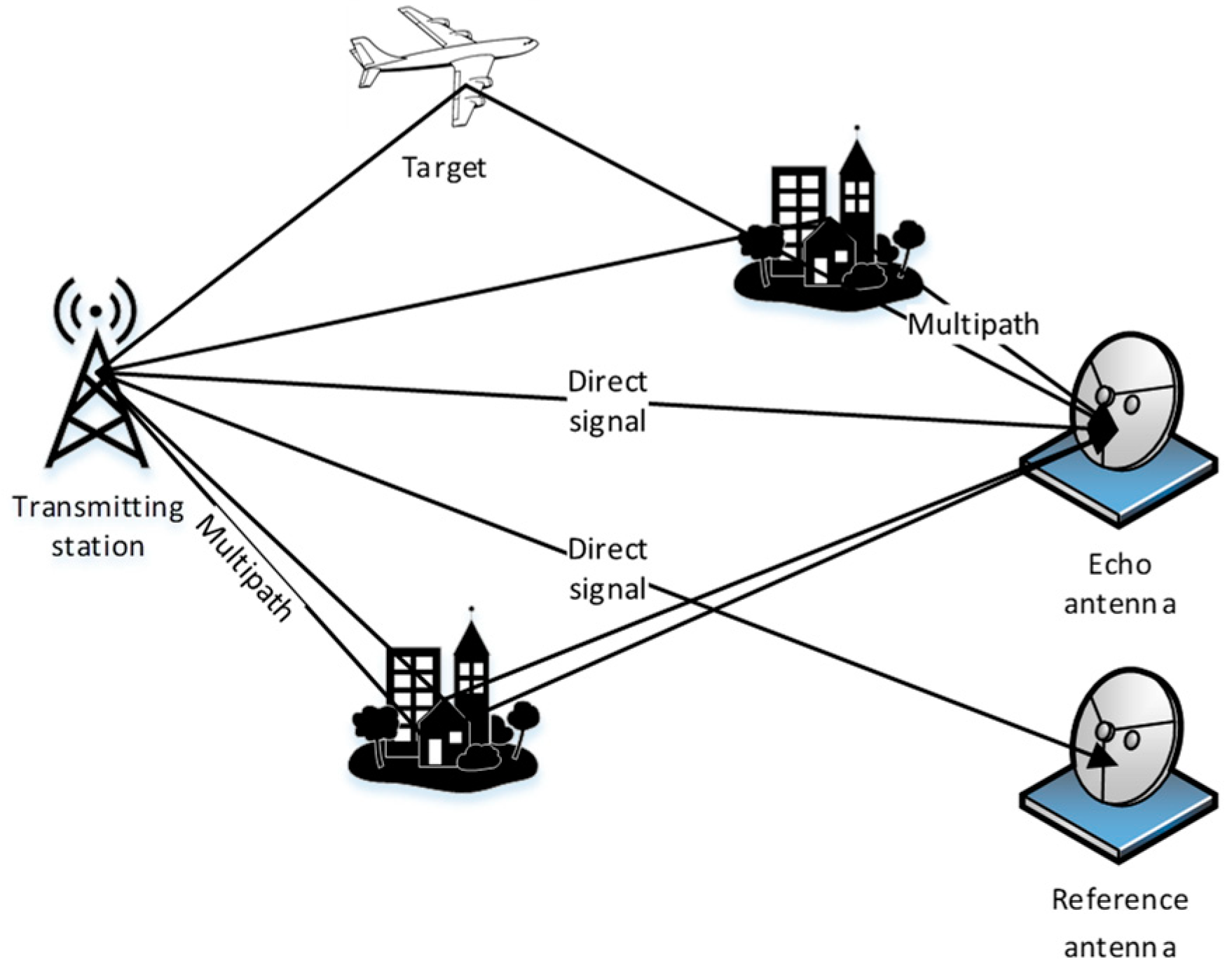
The schematic of the passive system is shown in Figure 1.

After the signal is received by the reference antenna, it is converted to the digital base band through analog to digital conversion, digital down conversion, filtering extraction, and other operations. Assume that the reference signal only contains reference signal and noise, it can be described as follows:

$$\begin{array}{cc}{s}_{ref}[n]=A_{ref}d[n]+z_{ref}[n]& n=1,\dots ,N\end{array}$$

(1)

where $d[n]$ indicates the n-th sampling of the direct wave signal of the transmitting station; $A_{ref}$ represents the complex amplitude of the direct wave signal received by the reference antenna; $z_{ref}$ represents the noise in the reference antenna; and N represents the length of the received signal.

Similarly, after the signal received by the echo antenna is converted into the digital base band, it can be described as follows:

$$x_{sur}[n]={\displaystyle \sum _{i=1}^{N_i}{A}_{i}d[n-{\lambda }_i]}+{\displaystyle \sum _{m=1}^{N_M}{a}_{m}d[n-{\lambda }_m]}{e}^{j2\pi f_{dm}\frac{n}{f_s}}+z_{sur}[n]\hspace{1em}n=1,,N$$

(2)

where $N_i$, $N_M$, and $N$, respectively, represent the number of clutter multi-paths, the number of targets, and the length of the signal sequence. $A_i$ and ${\lambda }_i$ are the complex amplitude of the i-th interference and the delay unit relative to the direct wave signal of the base station. The interference includes direct wave, multi-path, and other types of clutter, where ${\lambda }_1=0$ indicates that the first interference is a direct wave from the base station. $a_m$, ${\lambda }_m$, and $f_{dm}$, respectively, represent the complex amplitude, time delay, and Doppler frequency shift of the m-th target echo. $z_{sur}[n]$ represents the noise in the received signal of the echo antenna, and $f_s$ represents the sampling rate.

Because the direct wave and multi-path interference is much stronger than the target echo signal, interference cancellation is needed before target detection. In this paper, the ECA algorithm is used to cancel the interference of the echo signal [5]. The signal produced after interference cancellation can be expressed as follows:

$$s_{sur}[n]={\displaystyle \sum _{m=1}^{N_M}{a}_{m}d[n-{\lambda }_m]}{e}^{j2\pi f_{dm}\frac{n}{f_s}}+z_{sur}[n]$$

(3)

where the Doppler domain interval is $1/f_s$.

2.2. Algorithm Description and Analysis

After interference cancellation, the reference signal and multi-path interferences are eliminated. However, the target echo signal is still hidden in the noise background, which means that it is difficult to achieve target detection. Therefore, further processing is needed to improve the target SNR. Traditional target detection methods use R-D processing to improve the output SNR of the target echo signal.

2.2.1. Traditional Cross-Correlation Algorithm

In traditional target detection, R-D processing is usually adopted. This is realized by using the two-dimensional correlation between the reference signal and the echo signal as follows:

$$\chi [\lambda ,f]={\displaystyle \sum _{n=1}^N{s}_{sur}[n]s_{ref}^{*}[n-\lambda ]e^{-j2\pi f\frac{n}{f_s}}}$$

(4)

when $\lambda ={\lambda }_m$ and $f=f_m$, the correlation between the reference signal and the echo signal reaches the maximum value. The m-th target obtains the main lobe peak value corresponding to $\left[{\lambda }_m,f_{dm}\right]$. Then, the CFAR algorithm is used to detect the target on the R-D plane obtained by the above formula and the parameters of the target are obtained at the same time.

2.2.2. Novel Cross Correlation Algorithm

In this paper, a novel cross correlation processing method is proposed. First, the received echo signal and reference signal are converted into multiple signals by differential operations. At this time, there is a phase difference between the target part and the noise part of the multi-channel signals, so coherent integration between the multi-channel signals cannot be achieved. Therefore, through frequency domain processing, this paper transforms the target part of each channel signal into an in-phase signal and the interference and noise part into a non-in-phase signal, thus realizing the twice coherent processing of multiple target signals and greatly improving the target output SNR. The specific treatment scheme is as follows:

The reference signal and echo signal will be differentiated as follows:

$$\begin{array}{l}{r}_{ref}[l,n]=s_{ref}[n]s_{ref}^{*}[n-l]\\ ={\left|A_{ref}\right|}^{2}d[n]d^{*}[n-l]+A_{ref}^{*}{z}_{ref}[n]d^{*}[n-l]+A_{ref}d[n]\cdot z_{ref}^{*}[n-l]+z_{ref}[n]z_{ref}^{*}[n-l]\\ n=1,\dots ,N,l=1,\dots ,N-1\end{array}$$

(5)

$$\begin{array}{l}{r}_{sur}[l,n]=s_{sur}[n]s_{sur}^{*}[n-l]\\ ={\displaystyle \sum _{m=1}^{N_M}{\left|a_m^{}\right|}^{2}d[n-{\lambda }_m]d^{*}[n-{\lambda }_m-l]e^{j2\pi f_{dm}\frac{l}{f_s}}}+{\displaystyle \sum _{m=1}^{N_M}{\displaystyle \sum _{c=1,c\ne m}^{N_M}{a}_m{a}_c^{*}d[n-{\lambda }_m]d^{*}[n-{\lambda }_c-l]e^{j2\pi f_{dm}\frac{n}{f_s}}{e}^{-j2\pi f_{dc}(\frac{n}{f_s}-\frac{l}{f_s})}}}\\ +{\displaystyle \sum _{m=1}^{N_M}{a}_m^{*}{z}_{sur}[n]d^{*}[n-{\lambda }_m-l]e^{-j2\pi f_{dm}(\frac{n}{f_s}-\frac{l}{f_s})}}+{\displaystyle \sum _{m=1}^{N_M}{a}_m{z}_{sur}^{*}[n-l]d[n-{\lambda }_m]e^{j2\pi f_{dm}(\frac{n}{f_s})}}+z_{sur}^{*}[n-l]z_{sur}[n]\\ n=1,\dots ,N,l=1,\dots ,N-1 \end{array}$$

(6)

where $l={\tau }_l{f}_s$. $r_{ref}[l,n]$, $r_{sur}[l,n]$, respectively, represent the l-order difference of the reference signal and the echo signal (that is, to multiply the corresponding point between the signal and the signal after time delay) and l is an integer less than N. * represents the conjugation of the signal. In (6), the first term represents the conjugate point multiplication of the same target signal and its signal after l-order delay. The second term represents the conjugate point multiplication of the m-th target signal and the c-th target signal after l-order delay.

It can be seen from (6) that after the differential operation, in the first term, the Doppler frequency offset of the target echo becomes a constant term with l.

Then, we assume

$$p_l(n)=d[n]d^{*}[n-l]$$

(7)

Equations (5) and (6) can be written as follows:

$$\begin{array}{c}{r}_{ref}[l,n]=s_{ref}[n]\cdot s_{ref}^{*}[n-l]={\left|A_{ref}\right|}^2{p}_l[n]+z_{r,r}(l,n)\\ n=1,\dots ,N,l=1,\dots ,N-1\end{array}$$

(8)

where $z_{r,r}[l,n]=A_{ref}^{*}{z}_{ref}[n]d^{*}[n-l]+A_{ref}d[n]\cdot z_{ref}^{*}[n-l]+z_{ref}[n]z_{ref}^{*}[n-l]$.

$$\begin{array}{c}{r}_{sur}[l,n]=s_{sur}[n]\cdot s_{sur}^{*}[n-l]={\displaystyle \sum _{m=1}^{N_M}{\left|a_m\right|}^2{e}^{j2\pi f_{dm}\frac{l}{f_s}}{p}_l\left[n-{\lambda }_m\right]}+\zeta \left[l,n\right]\\ n=1,\dots ,N,l=1,\dots ,N-1\end{array}$$

(9)

where

$$\begin{array}{l}\zeta \left[l,n\right]={\displaystyle \sum _{m=1}^{N_M}{\displaystyle \sum _{c=1,c\ne m}^{N_M}{a}_m{a}_c^{*}d[n-{\lambda }_m]d^{*}[n-{\lambda }_c-l]e^{j2\pi f_{dm}\frac{n}{f_s}}{e}^{-j2\pi f_{dc}(\frac{n}{f_s}-\frac{l}{f_s})}}}\\ +{\displaystyle \sum _{m=1}^{N_M}{a}_m^{*}{z}_{sur}[n]d^{*}[n-{\lambda }_m-l]e^{-j2\pi f_{dm}(\frac{n}{f_s}-\frac{l}{f_s})}}+{\displaystyle \sum _{m=1}^{N_M}{a}_m{z}_{sur}^{*}[n-l]d[n-{\lambda }_m]e^{j2\pi f_{dm}(\frac{n}{f_s})}}+z_{sur}^{*}[n-l]z_{sur}[n]\\ n=1,\dots ,N,l=1,\dots ,N-1\end{array}$$

(10)

The Fourier transformation of (8) and (9) results in (11) and (12):

$$\begin{array}{c}{R}_{ref}[l,k]=FFT\left(r_{ref}(l,n)\right)={\left|A_{ref}\right|}^2{P}_l(k)+Z_{r,r}(l,k)\\ k=1,\dots ,N,l=1,\dots ,N-1\end{array}$$

(11)

where $FFT(\cdot )$ represent the Fourier transform and $P_l(k)$, $Z_{r,r}(l,k)$ represent the Fourier transform of $p_l(n)$, $z_{r,r}(l,n)$, respectively.

$$R_{sur}[l,k]=FFT\left[r_{sur}(l,n)\right]={\displaystyle \sum _{m=1}^{N_M}{\left|a_m\right|}^2{e}^{j2\pi f_{dm}\frac{l}{f_s}}{P}_l(k)e^{-j2\pi {\lambda }_{m}k}}+FFT\left(\zeta \left[l,n\right]\right)$$

(12)

Multiplying the conjugate points of (11) and (12) gives

$$R[l,k]=R_{sur}[l,k]R_{ref}^{*}[l,k]={\left|A_{ref}\right|}^2{\displaystyle \sum _{m=1}^{N_M}{\left|a_m\right|}^2{e}^{j2\pi f_{dm}\frac{l}{f_s}}{P}_l(k)P_l^{*}(k)e^{-j2\pi {\lambda }_{m}k}}+H(l,k)$$

(13)

where $H(l,k)$ is shown as follows:

$$H[l,k]=Z_{r,r}^{*}(l,k)\cdot {\displaystyle \sum _{m=1}^{N_M}{\left|a_m\right|}^2{e}^{j2\pi f_{dm}\frac{l}{f_s}}{P}_l(k)e^{-j2\pi {\lambda }_{m}k}}+Z_{r,r}^{*}(l,k)\cdot FFT\left(\zeta \left[l,n\right]\right)+{\left|A_{ref}\right|}^2{P}_l^{*}(k)\cdot FFT\left(\zeta \left[l,n\right]\right)$$

(14)

As can be seen from Equation (13), the phase of the transmitted signal contained in the first item is eliminated and transformed into a constant sequence $P_l(k)P_l^{*}(k)$, and there are only complex phases caused by the target delay and Doppler. Thus, in ${\left|A_{ref}\right|}^2{\displaystyle \sum _{m=1}^{N_M}{\left|a_m\right|}^2{e}^{j2\pi f_{dm}\frac{l}{f_s}}{P}_l(k)P_l^{*}(k)e^{-j2\pi {\lambda }_{m}k}}$, there are phase differences $e^{-j2\pi {\lambda }_{m}k}$ that are only related to the time delay for various differential orders l and there are phase differences $e^{j2\pi f_{dm}\frac{l}{f_s}}$ only related to the frequency offset for different sampling points k.

After searching and compensating for the time delay and frequency offset under various differential orders l,

$$\begin{array}{c}{R}_l[k,f,\lambda ]=R[l,k]e^{-j2\pi f\frac{l}{f_s}}{e}^{j2\pi \lambda k}\hfill \\ \hspace{1em}\hspace{1em}\hspace{1em}\hspace{1em}={\left|A_{ref}\right|}^2{\displaystyle \sum _{m=1}^{N_M}{\left|a_m\right|}^2{e}^{j2\pi (f_{dm}-f)\frac{l}{f_s}}{P}_l(k)P_l^{*}(k)e^{-j2\pi ({\lambda }_m-\lambda )f_{s}k}}+H(l,k)e^{-j2\pi f\frac{l}{f_s}}{e}^{j2\pi \lambda k}\end{array}$$

(15)

By taking k as a variable and accumulating $R_l\left[k,f,\tau \right]$ under various differential orders l, the following can be obtained:

$$\begin{array}{l}{R}_l[f,\lambda ]={\displaystyle \sum _{k=1}^N{R}_l\left[k,f,\lambda \right]}\\ ={\left|A_{ref}^{}\right|}^2{\displaystyle \sum _{m=1}^{N_M}{\displaystyle \sum _{k=1}^N{\left|a_m^{}\right|}^2{P}_l(k)P_l^{*}(k)e^{j2\pi (f_{dm}-f)\frac{l}{f_s}}{e}^{-j2\pi ({\lambda }_m-\lambda )f_{s}k}}}+{\displaystyle \sum _{k=1}^{N}H(l,k)e^{-j2\pi f\frac{l}{f_s}}{e}^{j2\pi {\lambda }_{s}k}}\\ ={\displaystyle \sum _{m=1}^{N_m}\left[{\left|A_{ref}^{}\right|}^2{\left|a_m^{}\right|}^2{e}^{j2\pi (f_{dm}-f)\frac{l}{f_s}}{\displaystyle \sum _{k=1}^N{D}_l{e}^{-j2\pi ({\lambda }_m-\lambda )f_{s}k}}\right]}+{\displaystyle \sum _{k=1}^{N}H(l,k)e^{-j2\pi f\frac{l}{f_s}}{e}^{j2\pi \lambda k}}\end{array}$$

(16)

where D_l is a constant sequence, $D_l=P_l(k)P_l^{*}(k)$.

From Equation (15), it is shown that there is a phase difference in ${\displaystyle \sum _{k=1}^{N}H(l,k)e^{-j2\pi f\frac{l}{f_s}}{e}^{j2\pi \lambda k}}$ at different sampling points k or differential orders l. When Equation (16) is carried out with different l values, Equation (17) is obtained,

$$\begin{array}{c}V={\displaystyle \sum _{l=1}^{N-1}{R}_l\left[f,\lambda \right]}\hfill \\ \hspace{1em}={\displaystyle \sum _{m=1}^{N_m}\left[{\left|A_{ref}\right|}^2{\left|a_m\right|}^2{\displaystyle \sum _{l=1}^{N-1}\left[e^{j2\pi (f_{dm}-f)\frac{l}{f_s}}\right]}{\displaystyle \sum _{k=1}^N{D}_l{e}^{-j2\pi ({\lambda }_m-\lambda )f_{s}k}}\right]}+{\displaystyle \sum _{l=1}^{N-1}{\displaystyle \sum _{k=1}^{N}H(l,k)e^{-j2\pi f\frac{l}{f_s}}{e}^{j2\pi \lambda k}}}\end{array}$$

(17)

When $\lambda ={\lambda }_m$ and $f=f_{dm}$, the maximum peak in Equation (17) is obtained, as shown in (18),

$$V_m={\left|A_{ref}\right|}^2{\left|a_m\right|}^2{\displaystyle \sum _{l=1}^{N-1}{D}_{sum,l}}+{\displaystyle \sum _{l=1}^{N-1}{\displaystyle \sum _{k=1}^{N}H(l,k)e^{-j2\pi f\frac{l}{f_s}}{e}^{j2\pi \lambda k}}}$$

(18)

where $D_{sum,l}={\displaystyle \sum _{k=1}^N{D}_l}$. The target echo becomes constant, allowing twice coherent accumulation to be achieved, whereas the noise and interference part achieves twice incoherent accumulation (the specific analysis can be seen in Part IV Algorithm Performance Analysis). Thus, the target time delay and Doppler can be accurately estimated. In order to realize the above delay Doppler compensation, the two-dimensional Fourier transform is adopted in this paper. For different orders l, the row vector takes the order l as the variable with a constant phase difference of $e^{-j2\pi {\lambda }_{m}k}$ and the column vector takes the discrete frequency k as the variable with a constant phase difference of $e^{j2\pi f_{dm}\frac{l}{f_s}}$. A two-dimensional matrix with l and k as the variables can be obtained through Equation (13), and the maximum dimensions of this matrix are given by the $(N-1)\times N$ dimensional matrix, as shown in (19),

$$\left[\begin{array}{ccc}R[1,1]& \cdots & R[1,N-1]\\ R[2,1]& \cdots & R[2,N-1]\\ ⋮& \ddots & ⋮\\ R[N-1,1]& \cdots & R[N-1,N-1]\\ R[N,1]& \cdots & R[N,N-1]\end{array}\right]$$

(19)

After a two-dimensional Fourier transform is performed in (19), we can obtain (20),

$$\begin{array}{l}Q[\lambda ,f]={\displaystyle \sum _{l=1}^{N-1}{\displaystyle \sum _{k=1}^{N}R(l,k)\exp \left[-j2\pi (f\frac{l}{f_s}+\lambda k)\right]}}\\ ={\displaystyle \sum _{l=1}^{N-1}{\displaystyle \sum _{k=1}^N\left\{A_{ref}^2{\displaystyle \sum _{m=1}^{N_M}\left\{a_m^2{D}_l{e}^{j2\pi (f-f_{dm})\frac{l}{f_s}}{e}^{-j2\pi ({\lambda }_m+\lambda )k}\right\}}+H(l,k)\exp \left[-j2\pi (f\frac{l}{f_s}+\lambda k)\right]\right\}}}\end{array}$$

(20)

where $\lambda$ and $f$ are the time delay and frequency offset search compensation factors, respectively, and (20) can be used to obtain the peak value when $f=f_{dm}$ and $\lambda ={\lambda }_m$ so as to obtain an accurate time delay and the Doppler estimation of the target.

3. Result

3.1. Simulation Data, Simulation Results, and Analysis

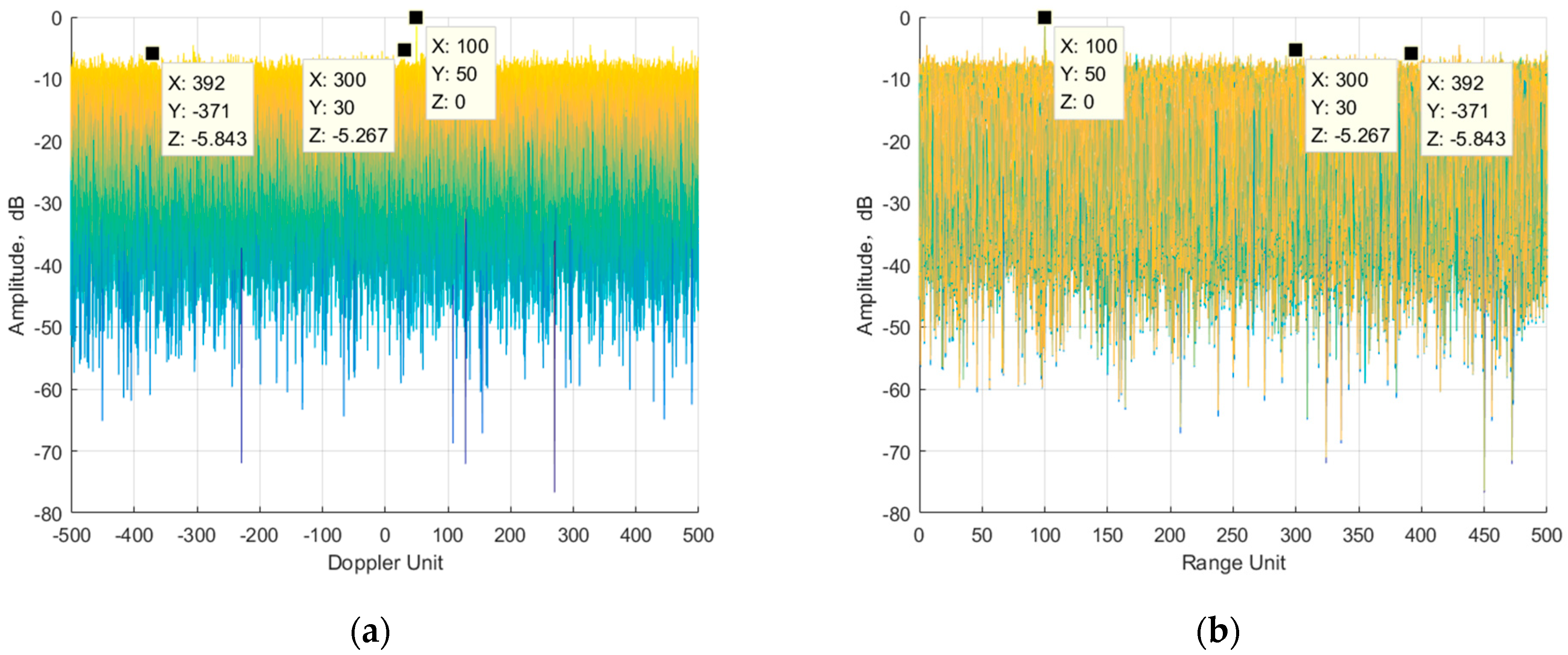
In this part, the transmitted signal is set as Gaussian white noise with length N. It is assumed that there is only the target echo and Gaussian white noise in the echo channel. Two targets are synthesized in the surveillance channel. The detailed parameter values are shown in

Table 1. Simulation Target Parameter.

	Range Unit	Doppler Unit	SNR
Tar 1	300	50	−25 dB
Tar 2	100	300	−30 dB

.

3.1.1. Simulation Analysis of Algorithm Performance with Pure Reference Signal

In this part, the sampling rate is set to 20 kHz and the accumulation time is 0.5 s. It is assumed that the reference channel is pure.

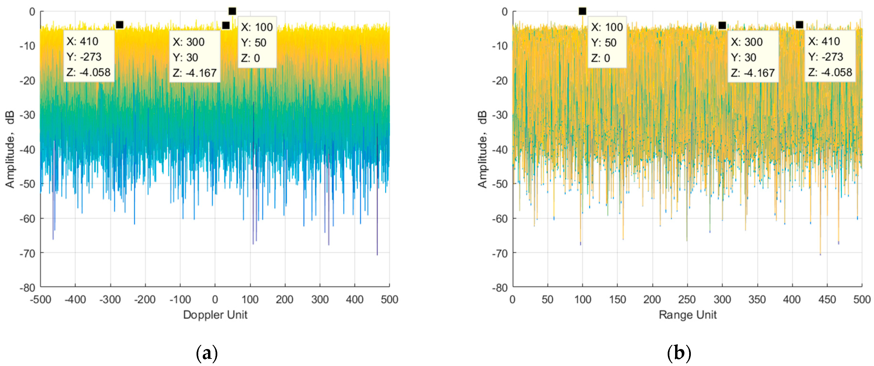
Figure 2 shows the results of traditional R-D processing, and Figure 3 gives the output SNR of the algorithm presented in this paper. It can be seen from Figure 2 that traditional R-D processing can only detect Tar1, which has a high SNR, and the integration gain is about 5.8 dB, whereas the small target is submerged under the noise floor. In Figure 3, the Tar1 output SNR in this paper is about 9.4 dB and the output SNR of Tar2 is about 4.4 db. Compared with the traditional R-D algorithm, the output SNR obtained in this paper is higher.

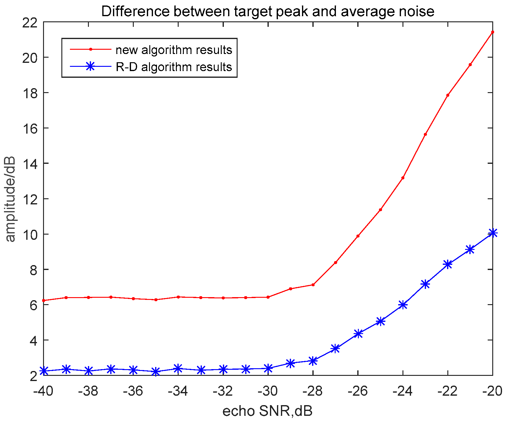
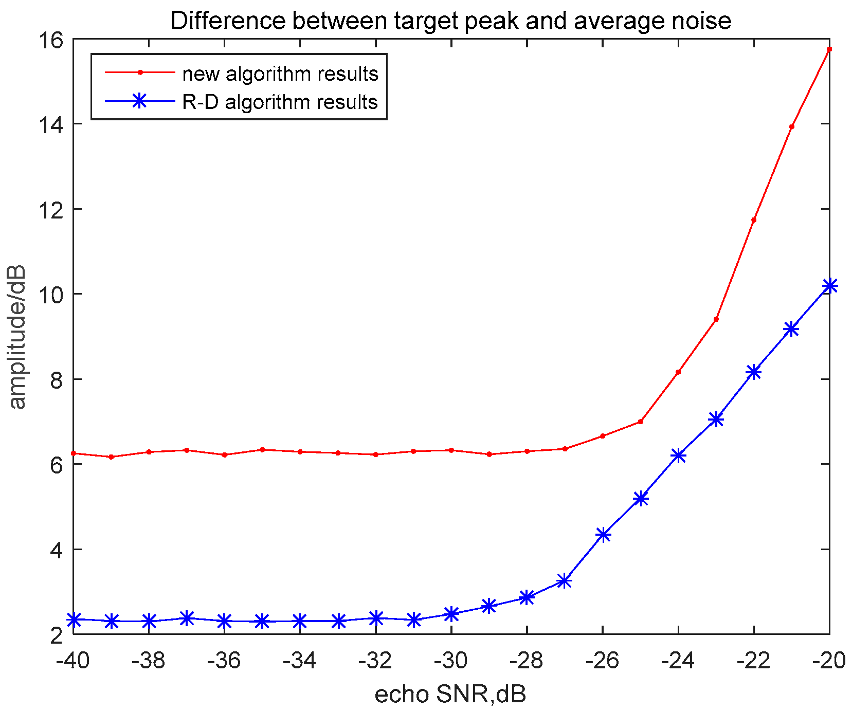
Figure 4 shows the difference comparison curve between the target peak value and mean noise platform value under different echo SNR with the pure reference signal. The point corresponding to each echo SNR in the figure is the result of 10,000 Monte Carlo simulations. It can be seen from the figure that the output SNR of the algorithm in this paper is much higher than that of the traditional R-D algorithm. With the increase of the echo SNR, the output SNR is improved faster.

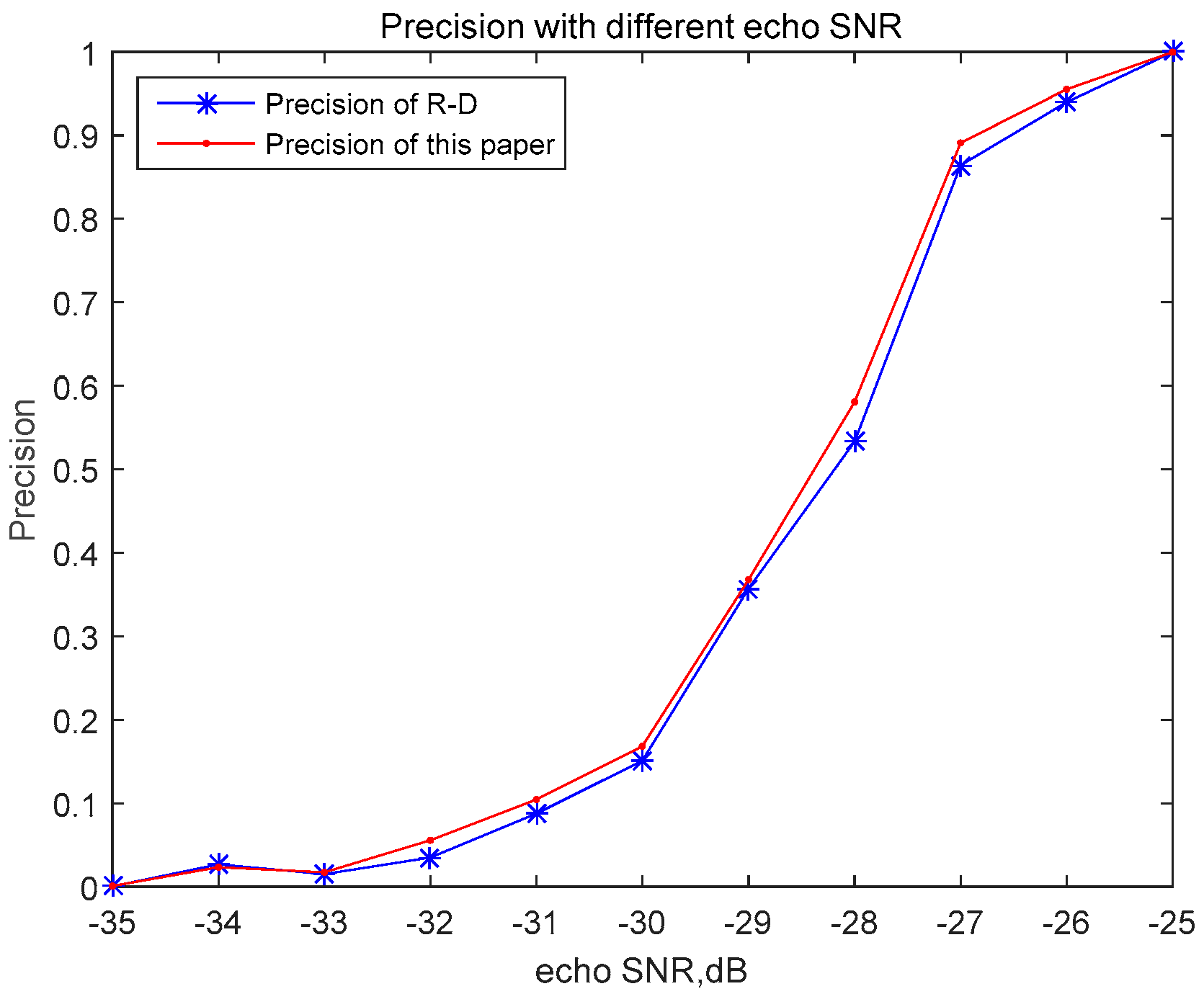
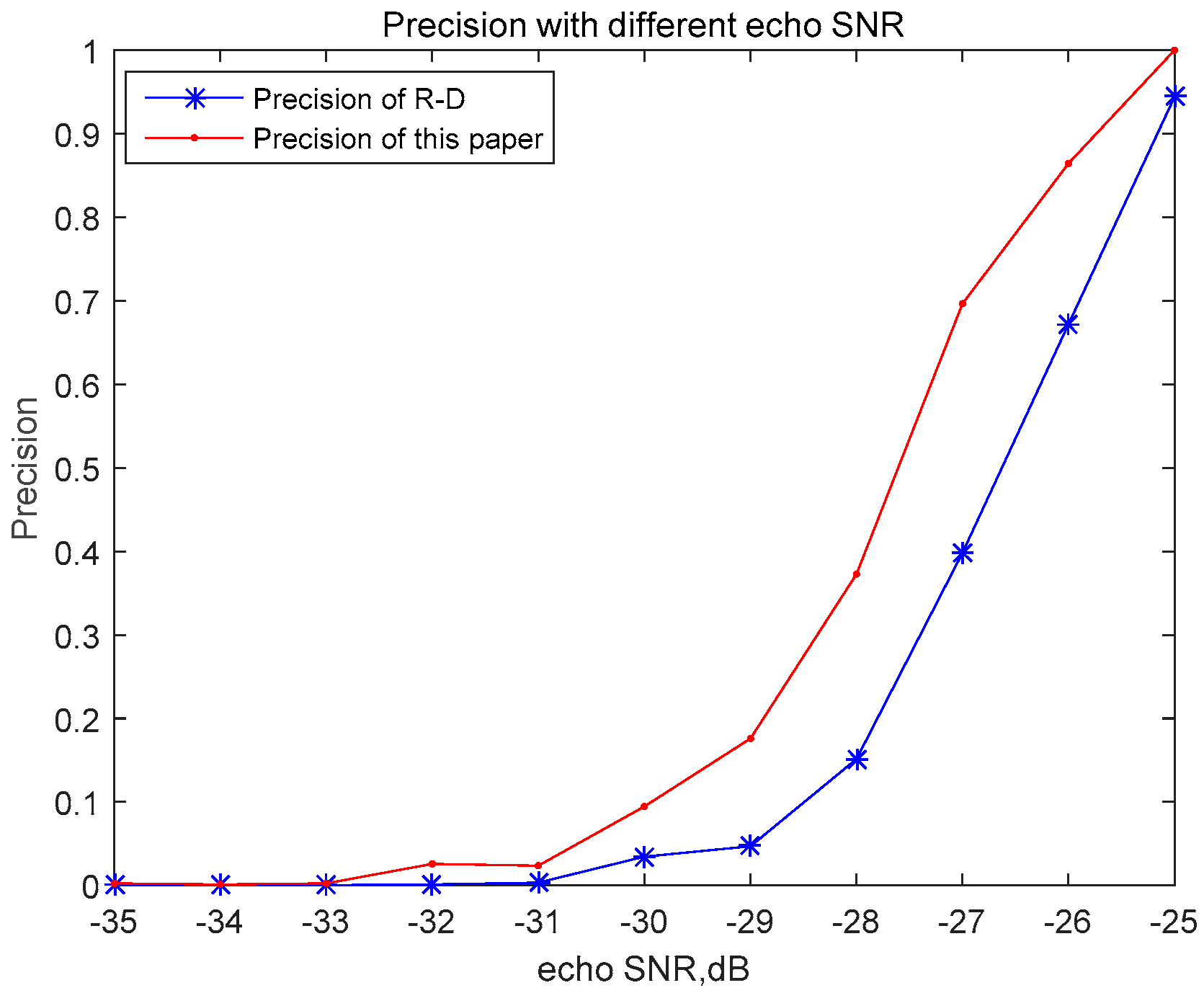
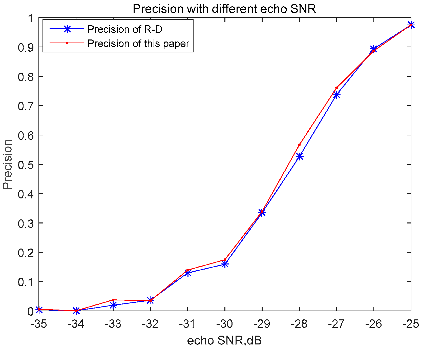
Figure 5 presents a comparison of precision values between the proposed algorithm and the R-D algorithm. The precision is defined as the proportion of the real target samples to all the predicted target samples. Under the condition that all targets can be detected, the threshold is set to be 0.5 dB less than the minimum target peak value. It can be seen from the figure that the precision of the algorithm presented in this paper is slightly higher than that of the traditional R-D algorithm.

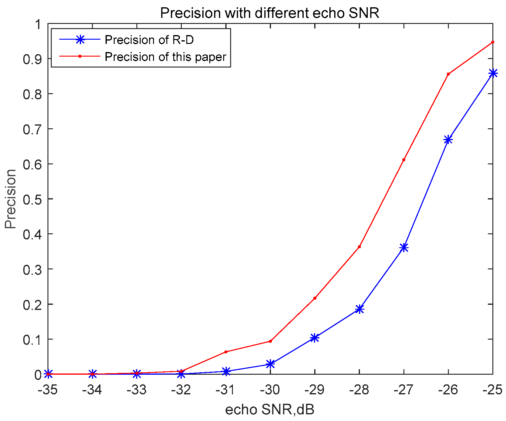
Compared with Figure 5, the threshold in Figure 6 is set to be 2 dB less than the minimum target peak value. It can be seen from the figure that the precision of the algorithm in this paper is much higher than that of the R-D algorithm.

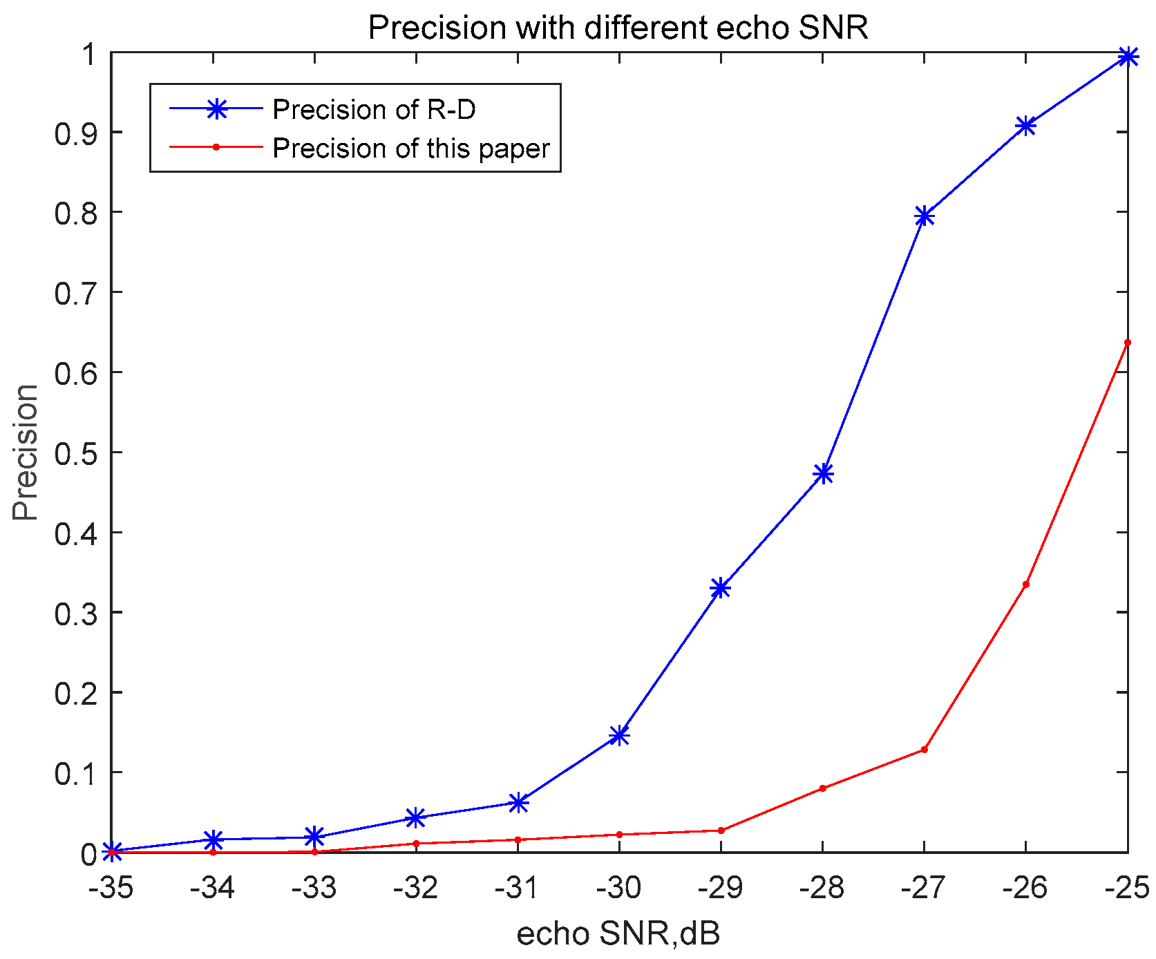
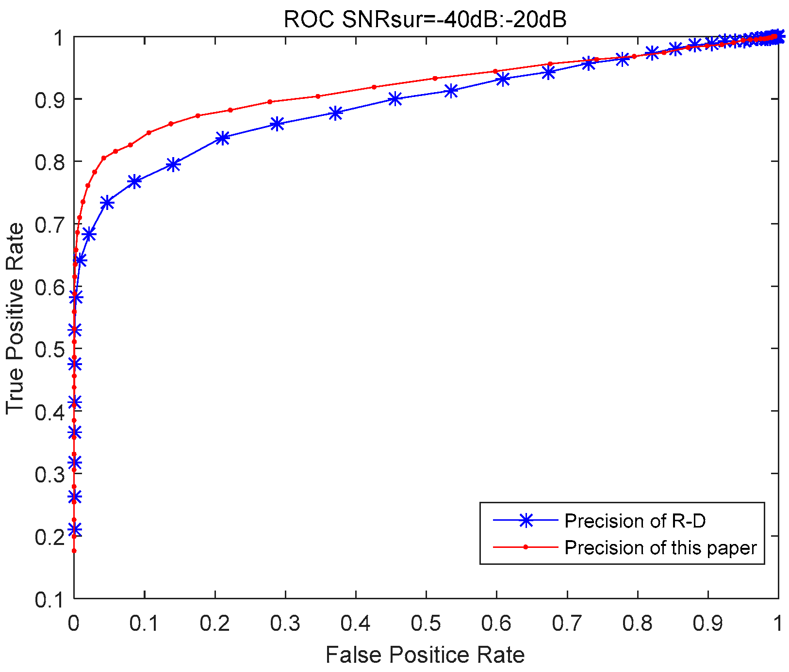
There are 10 targets in simulation of Figure 7, and their SNR is uniformly distributed in [−40 dB, −20 dB]. Each point in the figure has been subjected to 10,000 times Monte Carlo simulations. It can be seen from Figure 7 that the estimation performance of the algorithm in this paper is higher than that of the traditional R-D algorithm.

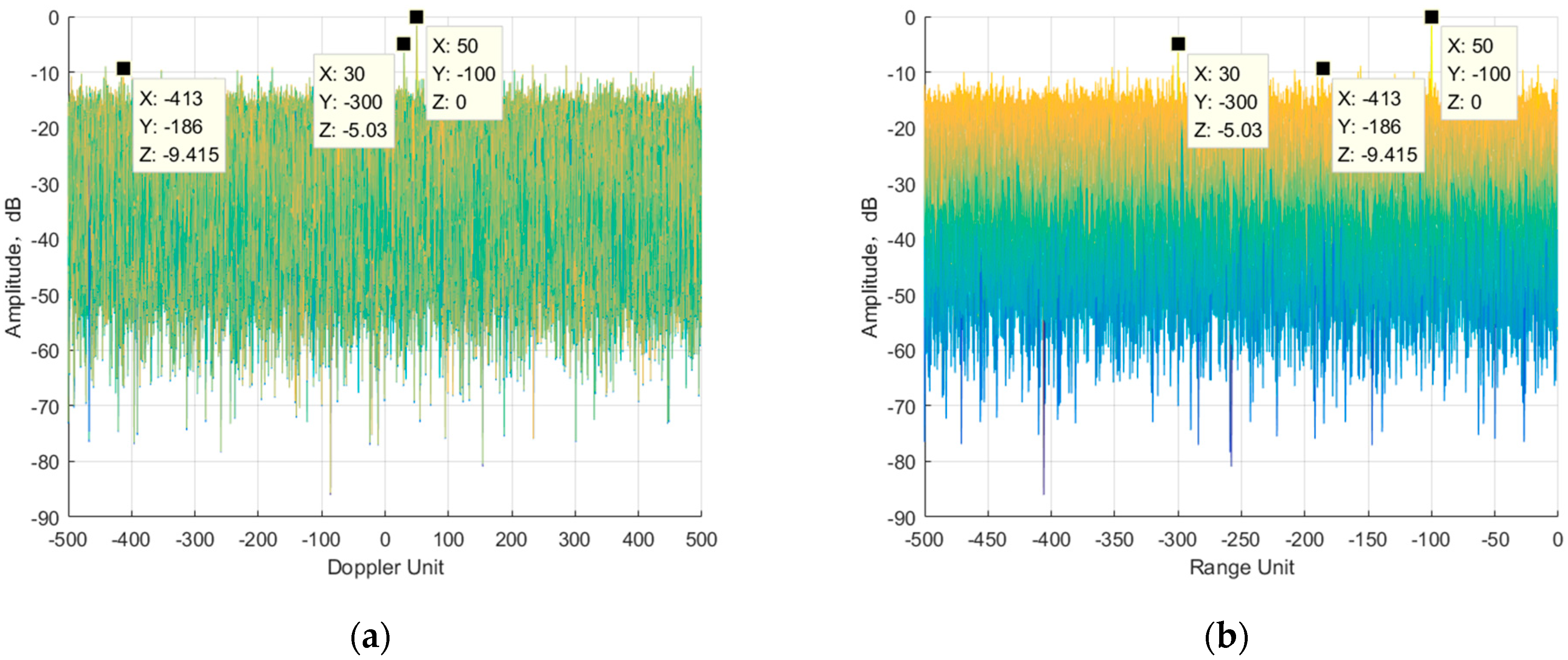
3.1.2. Simulation Analysis of the Algorithm’s Performance with Impure Reference Signal

In this part, the target parameters refer to the parameter settings presented in the previous section, as shown in Table 1. The reference channel is impure.

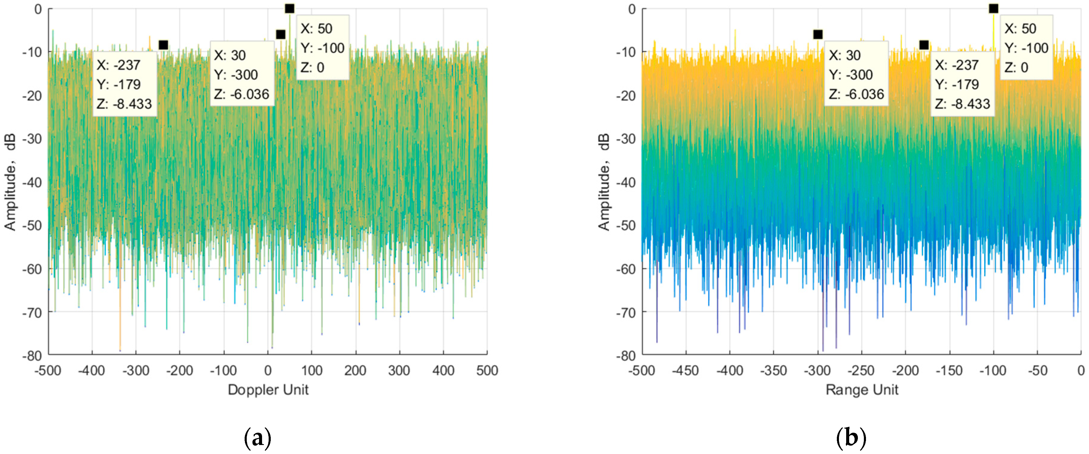
In Figure 8 and Figure 9, the SNR of the reference channel is set to 0 dB, and the signal length is $2\times {10}^4$. In Figure 8, the output SNR of Tar1 is about 4.16 dB and that of Tar2 cannot be detected. In Figure 9, the output SNR of Tar1 is about 8 dB and that of Tar2 is about 1.5 dB. Compared with the traditional algorithm, the proposed algorithm can detect smaller targets and the output SNR is higher.

Figure 10 presents the difference comparison curve between the target peak value and the mean noise platform value under different echo SNRs with 0 dB reference channel SNR. The point corresponding to each echo SNR in the figure is the result of 10,000 times Monte Carlo simulations. Compared with Figure 4, the output SNR of the algorithm presented in this paper is also much higher than that of the traditional R-D algorithm. With an increase in the echo SNR, the output SNR also improves.

Figure 11 presents the comparison of precision values between the proposed algorithm and the R-D algorithm with a reference SNR of 0 dB. Under the condition that all targets can be detected, the threshold is set to be 0.5dB less than the minimum target peak value. It can be seen from the figure that, similar to the results presented in Figure 5, the accuracy of the algorithm in this paper is higher than that of the traditional R-D algorithm. However, its estimation accuracy is slightly lower than that of the pure reference channel. Compared with Figure 11, the threshold in Figure 12 is set to be 2 dB less than the minimum target peak value. It can be seen from the figure that the precision of the algorithm in this paper is much higher than that of the R-D algorithm.

In Figure 13, the threshold is set to be 0.5 dB less than the minimum target peak value and the reference SNR is −10 dB. Compared with Figure 11, the estimation performance of the algorithm in this paper deteriorates rapidly when the reference SNR is lower. However, in the target detection of the passive radar, the reference antenna generally points directly to the transmitting base station, and its reference SNR is generally 0 dB or even higher. Therefore, in actual target detection, the estimation performance of this algorithm is generally higher than that of the traditional R-D algorithm.

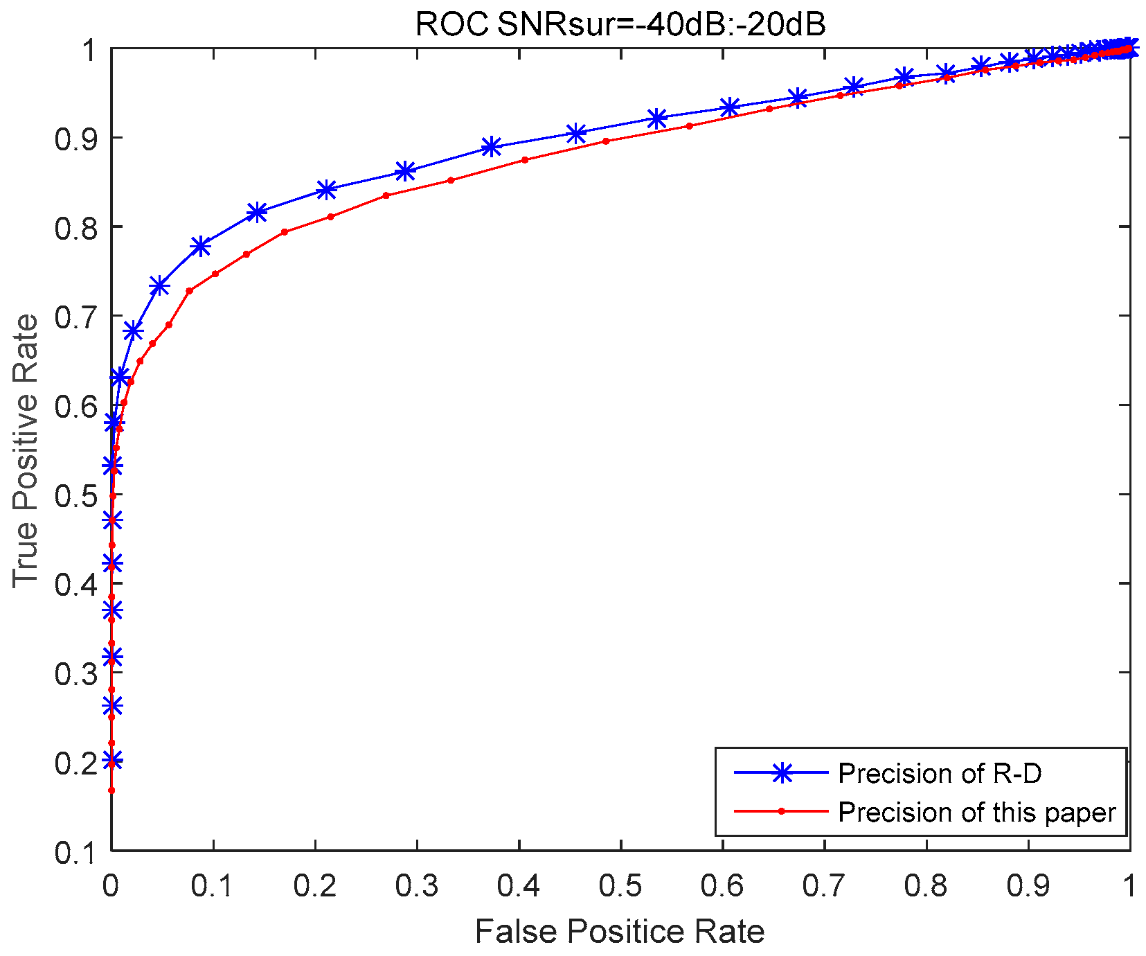
There are 10 targets in simulation of Figure 14 and Figure 15, and their SNR is uniformly distributed in [−40 dB, −20 dB]. Each point in the figure has been subjected to 10,000 Monte Carlo simulations. The SNR reference channel is 10 dB in Figure 14 and it is −5 dB in Figure 15. It can be seen from Figure 14 that the estimation performance of the algorithm in this paper is also higher than that of the traditional R-D algorithm. Compared with Figure 7, the results in Figure 14 are basically the same. That is, when the SNR of the reference channel is high, the estimation performance of the algorithm in this paper is basically not affected by the SNR of the reference channel. From the Figure 15, when the SNR of the reference channel is lower to −5 dB, the algorithm in this paper is greatly affected, and its estimation performance is lower than that of the traditional R-D algorithm. When the SNR of the reference channel is relatively lower, it may be necessary to use reference channel purification methods (such as reference reconstruction) to improve the SNR of the reference channel to ensure the algorithm performance.

In the above simulation, the output SNR did not reach the theoretical maximum, which was caused by the fact that the effective bandwidth of the signal could not be obtained accurately and the sampling rate was not equal to the effective bandwidth.

3.2. Measured Data, Measured Results, and Analysis

For the measurement of data, audio signals from China’s digital TV signal and FM broadcast signal were adopted. The echo signal and reference signal in the measured data were received by the echo antenna and the reference antenna, respectively, and the reference antenna points to the direction of the radiation source.

3.2.1. Measured Results and Analysis of the Audio Signal

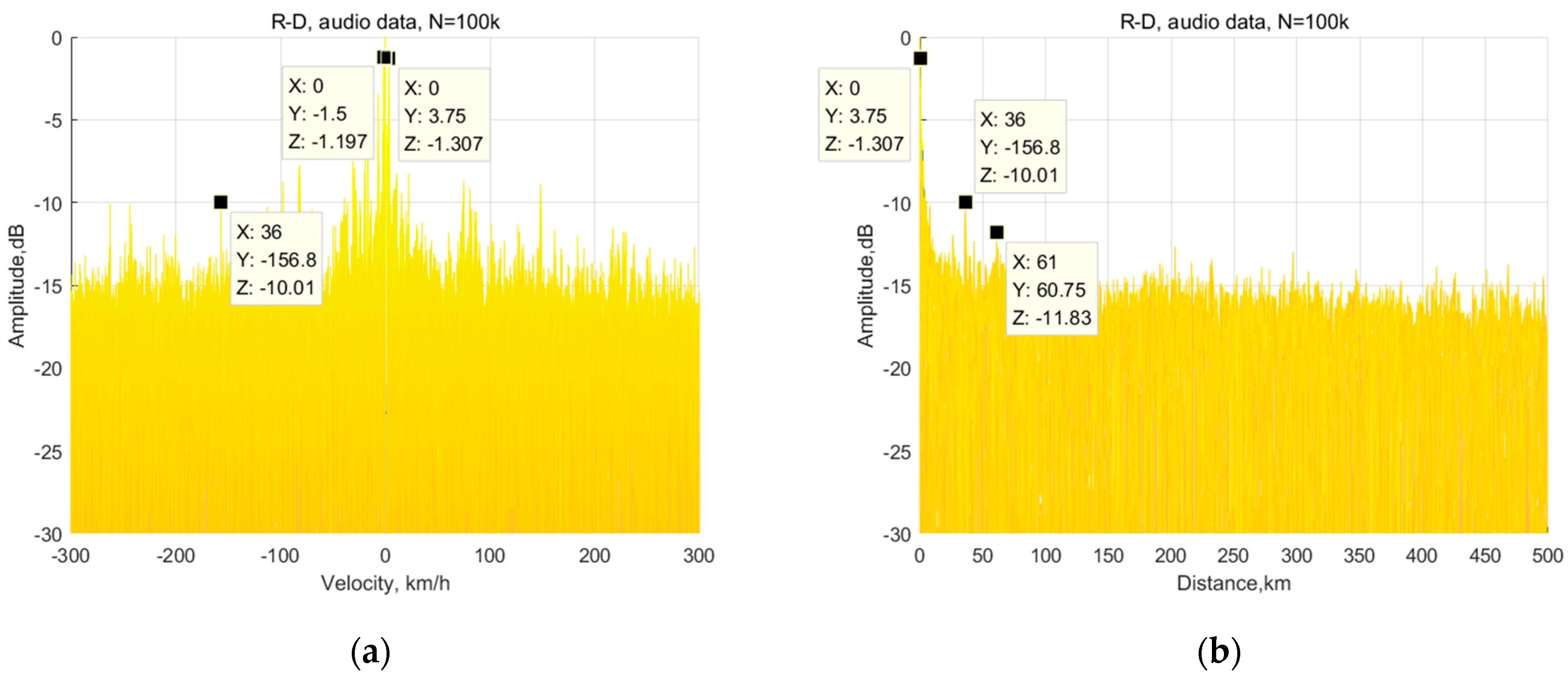
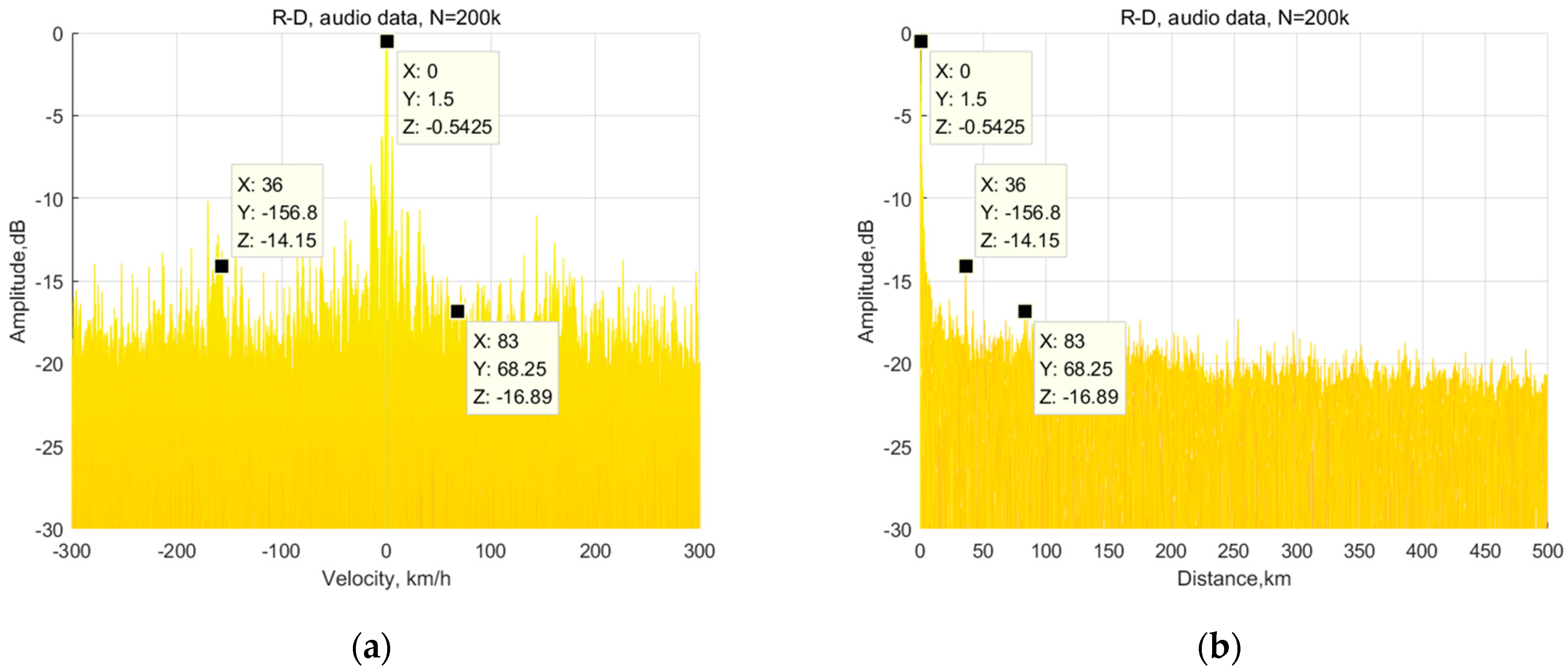
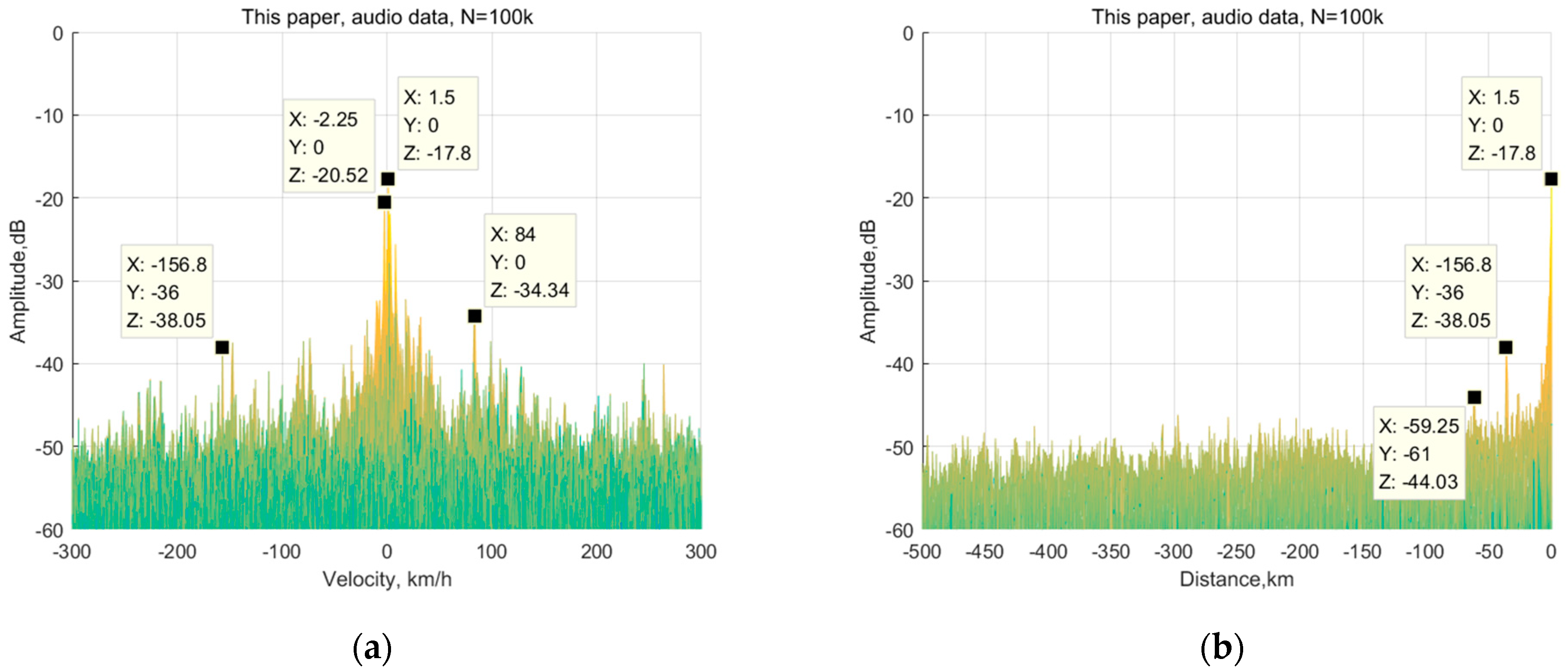
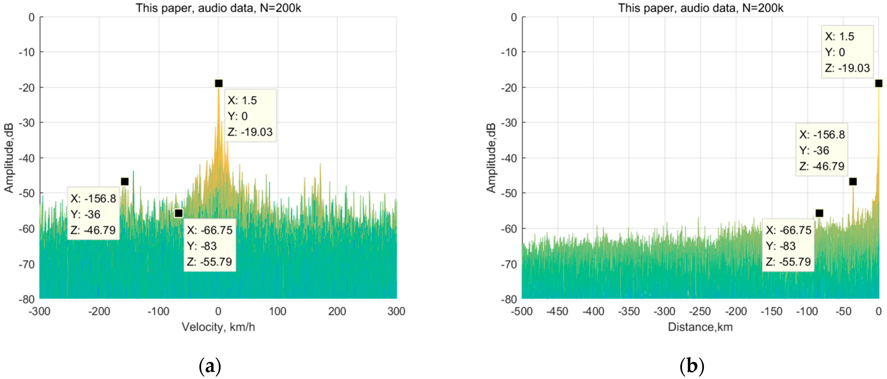
The effective bandwidth of the audio signal is within 130 kHz, the carrier frequency is 174.75 MHz, and the sampling frequency is 200 kHz. A total of seven frames of data were collected, and the length of each frame was 2.055 s. The target parameters were [36 km, −156.8 km/h]. During the simulation, the data in frame five were randomly selected, and the accumulation time was set to 0.5 s and 1 s, respectively. The Doppler resolution (that is, the Doppler frequency corresponding to each Doppler unit) was about 2 Hz and 1 Hz, respectively.

Figure 16a and Figure 17a show that there are many clutters with Doppler spread in the region near the receiver, so the target in Doppler dimension will be covered by the clutter. The estimated target position and Doppler presented in Figure 16b and Figure 17b are consistent, and the output SNR increases with an increase in the accumulation time. The output SNR of the target shown in Figure 16b and Figure 17b is about 2 dB and 2.8 dB, respectively.

As can be seen from Figure 18 and Figure 19, the algorithm in this paper can obtain the peak value in the Range–Doppler unit corresponding to the target. However, it is also affected by the clutter in the Doppler spread in the near region, and the target will be covered by clutter. When the accumulation time was 0.5 s, the output SNR of the algorithm in this paper was 6 dB, which is about 4 dB higher than the value shown in Figure 16. Similarly, when the accumulation time was 1s, the output SNR of the algorithm in this paper was 9 dB, which is about 6.2 dB higher than the value shown in Figure 17.

3.2.2. Measured Results and Analysis of the FM Signal

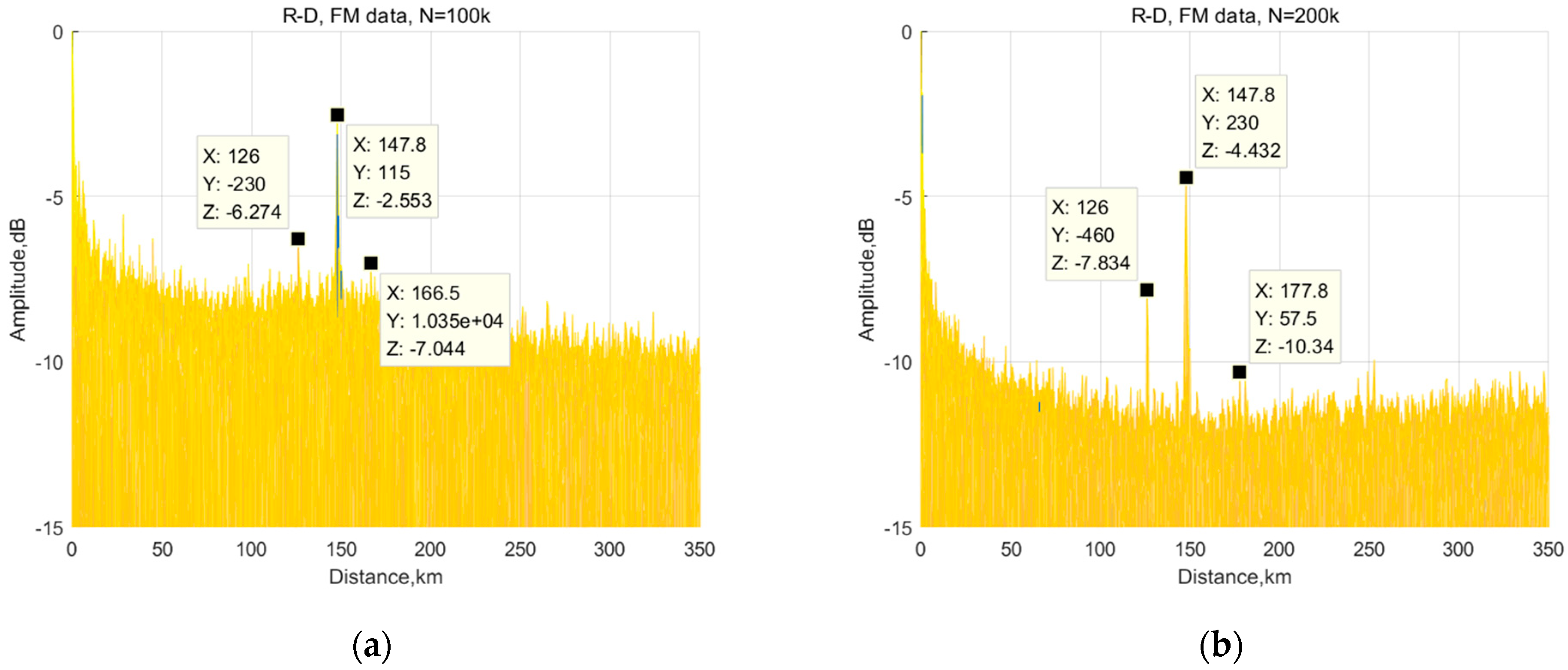
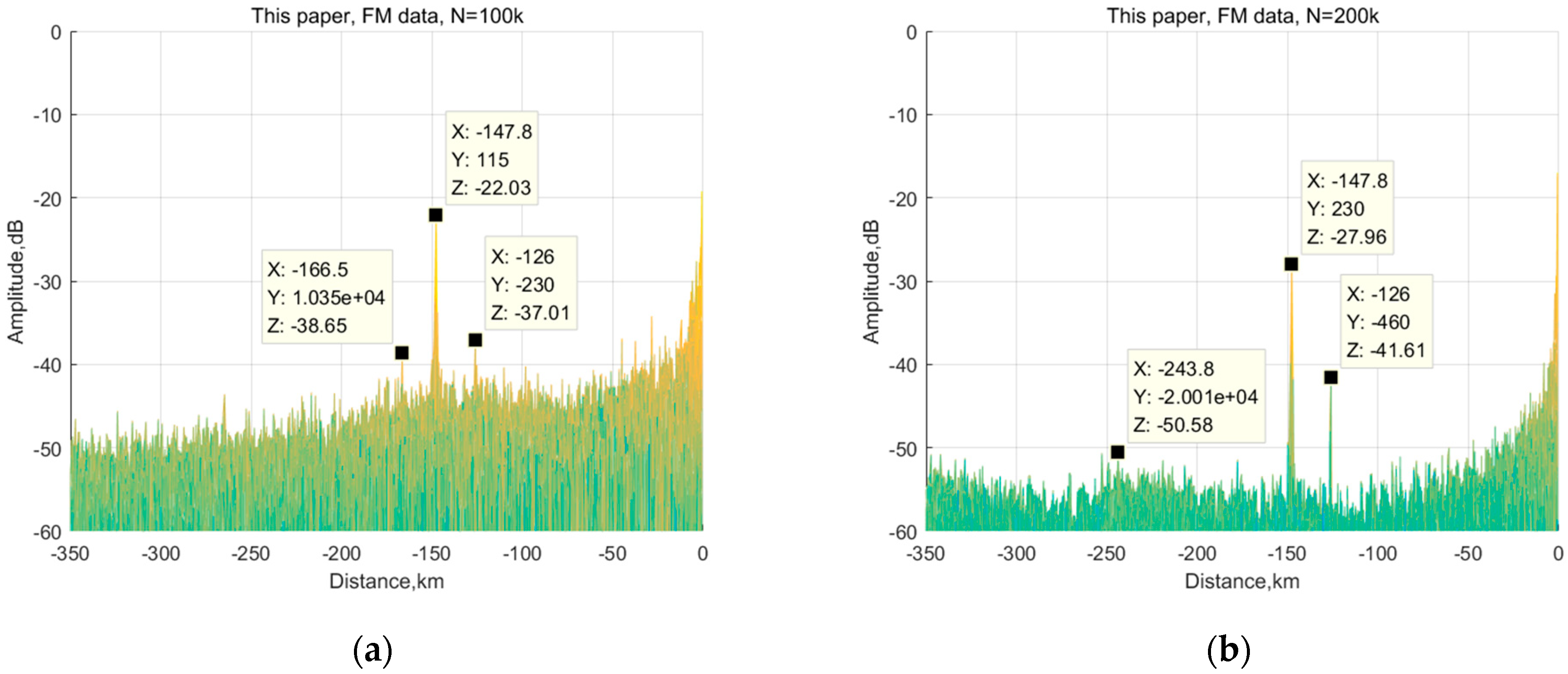
The effective bandwidth of the FM signal was within 75 kHz, the carrier frequency was 96.1 MHz, and the sampling frequency was 200 kHz. A total of seven frames of data were collected, and the length of each frame was 2 s. The target parameters were [336 km, −282.3 km/h] and [394 km, 64.1 km/h]. In the simulation, the data in the first frame were randomly selected and the accumulation times were 0.5 s and 1 s, respectively. Similar to audio signal data, FM signal data has many clutters with Doppler spread in the area close to the receiver and the target in the Doppler dimension will be covered by near-field clutter. Thus, only the distance dimension simulation results are given below.

It can be seen from Figure 20a,b that the output SNR of the target increases with the different accumulation time. When the accumulation time was 0.5 s, the traditional R-D output SNR of the two targets was about 4.5 dB and 0.8 dB, respectively. When the accumulation time was 1s, the traditional R-D output SNR of the two targets was about 5.9 dB and 2.5 dB, respectively. The improvement of output SNR in R-D processing is about 1.4 dB and 0.7 dB.

It can be seen from Figure 21a,b that when the accumulation time was 0.5 s, the two target output SNRs of the algorithm were about 15 dB and 1.6 dB. The output SNR was increased by about 10.5 dB and 0.8 dB, respectively, compared with the traditional R-D processing method in Figure 20. When the accumulation time was 1 s, the output SNRs of the two targets were about 23 dB and 9 dB, respectively, and the output SNR increased by about 16.1 dB and 6.5 dB compared with the traditional R-D processing method in Figure 20b.

When the accumulation time is short, the accumulation gain of this algorithm is higher than that of the traditional R-D algorithm. However, because the output SNR of the algorithm in this paper can be able to improve more for large targets, small targets will be affected by the sidelobe of large targets in short accumulation time accumulation, resulting in limited improvement. However, when the accumulation time increases, the output SNR of the algorithm is improved faster. Therefore, as shown in Figure 21a,b, when the accumulation time is twice the original time, the output SNR of the target in Figure 21b is about 12.5 dB and 8 dB higher than that in Figure 21a, while the traditional R-D algorithm, as shown in Figure 20a,b, is only about 1 dB higher (theoretically, the maximum increase can be about 3 dB).

4. Discussion

In the previous section, the simulation results of the proposed algorithm with the simulation data and the measured data were compared to the traditional R-D algorithm. In this section, we will theoretically deduce the output SNR of the two algorithms and give the final results to prove the effectiveness and the advantages of the proposed algorithm.

According to classical radar theory, when the sampling rate of the signal is $f_s=B$, the accumulation gain $G_c$ of the conventional CW radar can reach the maximum value, which is the product of the effective bandwidth B of the signal and the accumulation time T, $G_c=BT=N$.

The algorithm presented in this paper uses signal differential to transform a single channel signal into a multi-channel signal. Comparing Equations (3) with (6), the cross term is introduced into the differential signals, which results in a reduction in the SNR. The cross terms introduced are as follows:

$$\begin{array}{cc}\hfill r_{cross}[l,n]& ={\displaystyle \sum _{m=1}^{N_M}{a}_m{z}_{sur}^{*}[n-l]d[n-{\lambda }_m]e^{j2\pi f_{dm}(\frac{n}{f_s})}}+{\displaystyle \sum _{m=1}^{N_M}{a}_m^{*}{z}_{sur}[n]d^{*}[n-{\lambda }_m-l]e^{-j2\pi f_{dm}(\frac{n}{f_s}-\frac{l}{f_s})}}\hfill \\ & +{\displaystyle \sum _{m=1}^{N_m}{\displaystyle \sum _{c=1,c\ne m}^{N_m}\left\{\begin{array}{l}{a}_m{a}_{c}d[n-{\lambda }_m]d^{*}[n-{\lambda }_c-l]\\ \cdot e^{j2\pi (f_{dm}-f_{dc})\frac{n}{f_s}+f_{dc}\frac{l}{f_s}}\end{array}\right\}}}+z_{sur}^{*}[n-l]\cdot z_{sur}[n]\hfill \end{array}$$

(21)

Since the target energy is much lower than the signal noise energy, the above formula can be approximated as

$$\begin{array}{c}{r}_{cross}[l,n]\approx {\displaystyle \sum _{m=1}^{N_M}{a}_m^{*}{z}_{sur}[n]d^{*}[n-{\lambda }_m-l]e^{-j2\pi f_{dm}(\frac{n}{f_s}-\frac{l}{f_s})}}+{\displaystyle \sum _{m=1}^{N_M}{a}_m{z}_{sur}^{*}[n-l]d[n-{\lambda }_m]e^{j2\pi f_{dm}(\frac{n}{f_s})}}+z_{sur}^{*}[n-l]\cdot z_{sur}[n]\hfill \\ \hspace{1em}\hspace{1em}\hspace{1em}n=1,\dots ,N,l=1,\dots ,N-1\hfill \end{array}$$

(22)

The next step proves the correlation of $r_{cross}[l,n]$ with different orders l. According to the properties of Gaussian white noise, the auto-correlation function of Gaussian white noise is

$$W(\lambda )={\sigma }^2\delta (\lambda )=\left\{\begin{array}{c}{\sigma }^2\\ 0\end{array}\right.\begin{array}{c},\lambda =0\\ ,\lambda \ne 0\end{array}$$

(23)

Equation (22) shows that Gaussian noise is only related to itself and is completely irrelevant at any time difference; that is, $z_{sur}[n-l_1]$ is not related to $z_{sur}[n-l_2]$. Therefore, the third term on the right of (22) above is irrelevant under different orders l. When the signal to be processed is infinitely long, the multiplication of two Gaussian signals is still a Gaussian distribution, so the third terms on the right of (22) are independent of each other.

Table 2. Correlation coefficient.

	Correlation Coefficient
First item	0.2636
Second item	0.2686
Third item	0.0118
Gaussian white	0.0188

shows the correlation coefficient of each item in (22), where the differential order is $l=1$. The simulation results shown in Table 2 were attained with a Monte Carlo simulation (10,000 times). Table 2 shows that the correlation coefficient of the third term is closer to 0 than that of Gaussian white noise, so it can be regarded as uncorrelated. However, the correlation coefficients of the first and second terms are high. They cannot be regarded as completely irrelevant. However, the first and second terms represent a cross between the noise and signal and have little effect on the output SNR.

For the convenience of analysis, set $d[n]$ is the power to the normalized signal, the modulus of which is 1, and set $z_{ref}$ and $z_{sur}$ are the power to the normalized Gaussian white noise. Since the calculation of the accumulated gain is independent of the number of targets and the target echo energy is much lower than the noise energy, we assume that there is only one target in the echo signal (i.e., $N_m=1$ in (3)). Thus, the SNR of the reference channel before accumulation is $SN{R}_{ref\_RD}={\left|A_{ref}\right|}^2$. The SNR of the echo channel before accumulation is $SN{R}_{sur}={\left|a_1\right|}^2$.

Then, (4) is expanded as follows:

$$\begin{array}{l}\chi [\lambda ,f]={\displaystyle \sum _{n=1}^N{s}_{sur}[n]s_{ref}^{*}[n-\lambda ]e^{-j2\pi f\frac{n}{f_s}}}={\displaystyle \sum _{n=1}^N{A}_{ref}{a}_1{d}^{*}[n-\lambda ]d[n-{\lambda }_1]e^{j2\pi f_{d1}\frac{n}{f_s}}{e}^{-j2\pi f\frac{n}{f_s}}}+{\displaystyle \sum _{n=1}^N{A}_{ref}{d}^{*}[n-\lambda ]e^{-j2\pi f\frac{n}{f_s}}{z}_{sur}[n]}\\ +{\displaystyle \sum _{n=1}^N{a}_{1}d[n-{\lambda }_1]e^{j2\pi f_{d1}\frac{n}{f_s}}{z}_{ref}^{*}[n-\lambda ]e^{-j2\pi f\frac{n}{f_s}}}+{\displaystyle \sum _{n=1}^N{z}_{sur}[n]z_{ref}^{*}[n-\lambda ]e^{-j2\pi f\frac{n}{f_s}}}\end{array}$$

(24)

when $\tau ={\tau }_1$, $f=f_{d1}$, the peak appears at the target location,

$$\begin{array}{cc}\hfill {\left|\chi [{\lambda }_1,f_{d1}]\right|}^2& ={\left|{\chi }_{sr}[{\lambda }_1,f_{d1}]+{\chi }_{s{r}_z}[{\lambda }_1,f_{d1}]+{\chi }_{s_{z}r}[{\lambda }_1,f_{d1}]+{\chi }_{zz}[{\lambda }_1,f_{d1}]\right|}^2\hfill \\ & \approx \left|{\chi }_{sr}{[{\lambda }_1,f_{d1}]}^2+{\chi }_{s{r}_z}{[{\lambda }_1,f_{d1}]}^2+{\chi }_{s_{z}r}{[{\lambda }_1,f_{d1}]}^2+{\chi }_{zz}{[{\lambda }_1,f_{d1}]}^2\right|\hfill \end{array}$$

(25)

where

$${\chi }_{sr}[{\lambda }_1,f_{d1}]={\displaystyle \sum _{n=1}^N{A}_{ref}{a}_1{\left|d[n-{\tau }_1{f}_s]\right|}^2}=A_{ref}{a}_{1}N$$

(26)

$${\chi }_{r{s}_z}[{\lambda }_1,f_{d1}]={\displaystyle \sum _{n=1}^N{A}_{ref}{d}^{*}[n-{\tau }_1{f}_s]z_{sur}[n]e^{-j2\pi f_{d1}\frac{n}{f_s}}}$$

(27)

$${\chi }_{s{r}_z}[{\lambda }_1,f_{d1}]={\displaystyle \sum _{n=1}^N{a}_{1}d[n-\tau f_s]z_{ref}^{*}[n-{\tau }_1{f}_s]}$$

(28)

$${\chi }_{zz}[{\lambda }_1,f_{d1}]={\displaystyle \sum _{n=1}^N{z}_{sur}[n]z_{ref}^{*}[n-{\tau }_1{f}_s]e^{-j2\pi f_{d1}\frac{n}{f_s}}}$$

(29)

Since ${\chi }_{rz}$, ${\chi }_{sz}$, and ${\chi }_{zz}$ in the integral term can be regarded as stationary noise [30],

$${\chi }_{r{s}_z}[{\lambda }_1,f_{d1}]\approx A_{ref}\sqrt{N}$$

(30)

$${\chi }_{s{r}_z}[{\lambda }_1,f_{d1}]\approx a_1\sqrt{N}$$

(31)

$${\chi }_{zz}[{\lambda }_1,f_{d1}]\approx \sqrt{N}$$

(32)

4.1. Reference Signal without Noise

When the SNR of the reference channel is high or the reference channel is pure, the noise of reference channel can be ignored. The gain in coherent accumulation comes from the in-phase addition of N signal samples. The maximum gain in signal component energy is N², whereas out-phase signals can only achieve incoherent accumulation and the maximum accumulation gain is N.

From Formula (24), ignoring the reference channel noise, (24) can be rewritten as follows:

$${\left|\chi [{\lambda }_1,f_{d1}]\right|}^2\approx \left|{\chi }_{sr}{[{\lambda }_1,f_{d1}]}^2+{\chi }_{r{s}_z}{[{\lambda }_1,f_{d1}]}^2\right|$$

(33)

Then, the output SNR of the traditional R-D method is shown in (34):

$$G_{RD}=10{\log }_{10}(\frac{{\left|A_{ref}\right|}^2{\left|a_1\right|}^2{N}^2}{{\left|A_{ref}\right|}^{2}N})={\left|a_1\right|}^{2}N$$

(34)

For the algorithm in this paper, when the reference channel noise is ignored and there is only one target, Formula (13) can be written as,

$$\begin{array}{l}R[l,k]={\left|A_{ref}\right|}^2{\left|a_1\right|}^2{e}^{j2\pi f_{d1}\frac{l}{f_s}}{P}_l(k)P_l^{*}(k)e^{-j2\pi {\tau }_1{f}_{s}k}\\ +{\left|A_{ref}\right|}^2{P}_l^{*}(k)\cdot FFT\left(a_1^{*}{z}_{sur}[n]d^{*}[n-{\lambda }_1-l]e^{-j2\pi f_{d1}(\frac{n}{f_s}-\frac{l}{f_s})}+a_1{z}_{sur}^{*}[n-l]d[n-{\lambda }_1]e^{j2\pi f_{d1}(\frac{n}{f_s})}+z_{sur}^{*}[n-l]z_{sur}[n]\right)\end{array}$$

(35)

After compensating above time delay and frequency offset, the accumulate results can be obtained as follows:

$$\begin{array}{c}W[\lambda ,f]={\displaystyle \sum _{l=1}^{N-1}{\displaystyle \sum _{k=1}^{N}R(l,k)\exp \left[-j2\pi (f\frac{l}{f_s}+\lambda k)\right]}}\hfill \\ \hspace{1em}\hspace{1em}\hspace{1em}={\displaystyle \sum _{l=1}^{N-1}{\displaystyle \sum _{k=1}^N\left\{\begin{array}{l}{\left|A_{ref}^{}\right|}^2{\left|a_1^{}\right|}^2{P}_l(k)P_l^{*}(k)e^{j2\pi (f-f_{d1})\frac{l}{f_s}}{e}^{-j2\pi ({\lambda }_1+\lambda )k}\\ +{\left|A_{ref}^{}\right|}^2{P}_l^{*}(k)\cdot FFT\left(\begin{array}{l}{a}_1^{*}{z}_{sur}[n]d^{*}[n-{\lambda }_1-l]e^{-j2\pi f_{d1}(\frac{n}{f_s}-\frac{l}{f_s})}\\ +a_1{z}_{sur}^{*}[n-l]d[n-{\lambda }_1]e^{j2\pi f_{d1}(\frac{n}{f_s})}\\ +z_{sur}^{*}[n-l]z_{sur}[n]\end{array}\right)e^{j2\pi f\frac{l}{f_s}}{e}^{-j2\pi \lambda k}\end{array}\right\}}}\hfill \end{array}$$

(36)

when $\lambda =-{\lambda }_1$, $f=f_{d1}$, the peak appears at location of target 1:

$${\left|\eta [{\tau }_1,f_{d1}]\right|}^2\approx \left|{\eta }_{sr}{[{\tau }_1,f_{d1}]}^2+{\eta }_{s{r}_z}{[{\tau }_1,f_{d1}]}^2+{\eta }_{s_{z}r}{[{\tau }_1,f_{d1}]}^2+{\eta }_{zz}{[{\tau }_1,f_{d1}]}^2\right|$$

(37)

$${\left|{\eta }_{sr}[{\tau }_1,f_{d1}]\right|}^2={\displaystyle \sum _{l=1}^{N-1}{\displaystyle \sum _{k=1}^N\left\{{\left|A_{ref}\right|}^2{\left|a_1\right|}^2{P}_l(k)P_l^{*}(k)\right\}}}={\left|A_{ref}\right|}^4{\left|a_1\right|}^4{\left({\displaystyle \sum _{l=1}^{N-1}(N-l)}\right)}^2$$

(38)

The signal shown in Equation (38) has no phase difference after compensation and is a sequence of real numbers. Therefore, its coherent accumulation gain can be seen as a coherent accumulation of signal with data length ${\displaystyle \sum _{l=1}^{N-1}(N-l)}$.

$${\left|{\eta }_{zz}[\tau ,f]\right|}^2={\left\{{\displaystyle \sum _{l=1}^{N-1}{\displaystyle \sum _{k=1}^N\left\{{\left|A_{ref}\right|}^2{P}_l^{*}(k)\cdot FFT\left(z_{sur}^{*}[n-l]z_{sur}[n]\right)e^{j2\pi f\frac{l}{f_s}}{e}^{-j2\pi \tau f_{s}k}\right\}}}\right\}}^2$$

(39)

Under the same differential order l, the signal of Equation (39) has phase difference between different sampling points, so its accumulation is incoherent. However, under different differential orders l, it can be seen from Table 2 that the correlation of the signal in Equation (39) is weak and it can be approximated as non-correlation. At this time, the signal in Equation (39) realizes two incoherent accumulations. Its accumulated gain is approximately the incoherent accumulated gain of the signal with length ${\displaystyle \sum _{l=1}^{N-1}(N-l)}$, as shown in Equation (40),

$${\left|{\eta }_{zz}[\tau ,f]\right|}^2\approx {\left|A_{ref}\right|}^4{\displaystyle \sum _{l=1}^{N-1}(N-l)}$$

(40)

$${\left|{\eta }_{r{s}_z}[{\tau }_1,f_{d1}]\right|}^2={\left\{{\displaystyle \sum _{l=1}^{N-1}{\displaystyle \sum _{k=1}^N\left\{{\left|A_{ref}\right|}^2{P}_l^{*}(k)\cdot FFT\left(a_1^{*}{z}_{sur}[n]d^{*}[n-{\lambda }_1-l]e^{-j2\pi f_{d1}(\frac{n}{f_s}-\frac{l}{f_s})}\right)e^{j2\pi f_{d1}\frac{l}{f_s}}{e}^{-j2\pi {\lambda }_{1}k}\right\}}}\right\}}^2$$

(41)

$${\left|{\eta }_{r{s}_z}[{\tau }_1,f_{d1}]\right|}^2={\left\{{\displaystyle \sum _{l=1}^{N-1}{\displaystyle \sum _{k=1}^N\left\{{\left|A_{ref}\right|}^2{P}_l^{*}(k)\cdot FFT\left(a_1^{*}{z}_{sur}[n]d^{*}[n-{\lambda }_1-l]e^{-j2\pi f_{d1}(\frac{n}{f_s}-\frac{l}{f_s})}\right)e^{j2\pi f_{d1}\frac{l}{f_s}}{e}^{-j2\pi {\lambda }_{1}k}\right\}}}\right\}}^2$$

(42)

The signal shown in Equations (41) and (42) has phase difference between different sampling points under the same differential order l. Therefore, the incoherent accumulation is realized under the same differential order l. There is a correlation under different differential orders. As shown in Table 1, when the signals of Equation (41) and (42) are completely correlated under different differential orders, the output SNR of the algorithm in this paper can reach the theoretical lower bound. Its accumulation gain is the sum of incoherent accumulation under the same differential order l and coherent accumulation gain under different differential orders, as shown in Equation (43) and (44) below:

$$\begin{array}{c}{\left|{\eta }_{r{s}_z}[\tau ,f]\right|}^2={\left|A_{ref}\right|}^4{\left|a_1\right|}^2\left\{(N-1){\displaystyle \sum _{l=1}^{N-1}(N-l)}-\left[1+2+3+\cdots +(N-1)\right]\right\}\hfill \\ \hspace{1em}\hspace{1em}\hspace{1em}\hspace{1em}\approx {\left|A_{ref}\right|}^4{\left|a_1\right|}^2(N-2){\displaystyle \sum _{l=1}^{N-1}(N-l)}\hfill \end{array}$$

(43)

$$\begin{array}{c}{\left|{\eta }_{s{r}_z}[\tau ,f]\right|}^2\approx {\left|A_{ref}\right|}^4{\left|a_1\right|}^2\left((N-1){\displaystyle \sum _{l=1}^{N-1}(N-l)}-\left[1+2+3+\cdots +(N-1)\right]\right)\hfill \\ \hspace{1em}\hspace{1em}\hspace{1em}\hspace{1em}\approx {\left|A_{ref}\right|}^4{\left|a_1\right|}^2(N-2){\displaystyle \sum _{l=1}^{N-1}(N-l)}\hfill \end{array}$$

(44)

In the above Formulas (43) and (44), it is assumed that the signals are completely correlated under different cancellation orders and the accumulation is equivalent to N-1 times of signal amplification. Therefore, the accumulation result is the incoherent accumulation gain of the signal with length ${\displaystyle \sum _{l=1}^{N-1}(N-l)}$ multiplied by N-1. However, due to the difference method, the signal lengths under different difference orders are different, and the influence of the signal length needs to be subtracted, so the result in the formula is obtained.

When the signal part in Equations (41) and (42) is completely uncorrelated under different differential orders, the output SNR of the algorithm in this paper can reach the theoretical upper bound. Its accumulated gain is the sum of incoherent accumulation at the same differential order l and incoherent accumulation gain at different differential orders, and its accumulated gain is approximately the incoherent accumulated gain of the signal with length ${\displaystyle \sum _{l=1}^{N-1}(N-l)}$, as shown in Formulas (45) and (46) below:

$${\left|{\eta }_{r{s}_z}[\tau ,f]\right|}^2\approx {\left|A_{ref}\right|}^4{\left|a_1\right|}^2{\displaystyle \sum _{l=1}^{N-1}(N-l)}$$

(45)

$${\left|{\eta }_{s{r}_z}[\tau ,f]\right|}^2\approx {\left|A_{ref}\right|}^4{\left|a_1\right|}^2{\displaystyle \sum _{l=1}^{N-1}(N-l)}$$

(46)

Therefore, the output SNR $G_{new}$ in this paper is as follows:

$$G_{lower}\le G_{new}\le G_{upper}$$

(47)

$$G_{lower}\approx 10{\log }_{10}\frac{{\left|a_1\right|}^4{({\displaystyle \sum _{l=1}^{N-1}l})}^2}{{\displaystyle \sum _{l=1}^{N-1}l}+2{\left|a_1\right|}^2(N-2){\displaystyle \sum _{l=1}^{N-1}l}}\approx 10{\log }_{10}\frac{{\left|a_1\right|}^4({\displaystyle \sum _{l=1}^{N-1}l})}{1+2{\left|a_1\right|}^2(N-2)}$$

(48)

$$G_{upper}\approx 10{\log }_{10}\frac{{\left|a_1\right|}^4{({\displaystyle \sum _{l=1}^{N-1}l})}^2}{{\displaystyle \sum _{l=1}^{N-1}l}+2{\left|a_1\right|}^2{\displaystyle \sum _{l=1}^{N-1}l}}\approx 10{\log }_{10}\frac{{\left|a_1\right|}^4({\displaystyle \sum _{l=1}^{N-1}l})}{1+2{\left|a_1\right|}^2}$$

(49)

where $G_{lower}$ represents the lower bound of the output SNR, and $G_{upper}$ represents the upper bound of the output SNR. The simulation results are shown in the Figure 2.

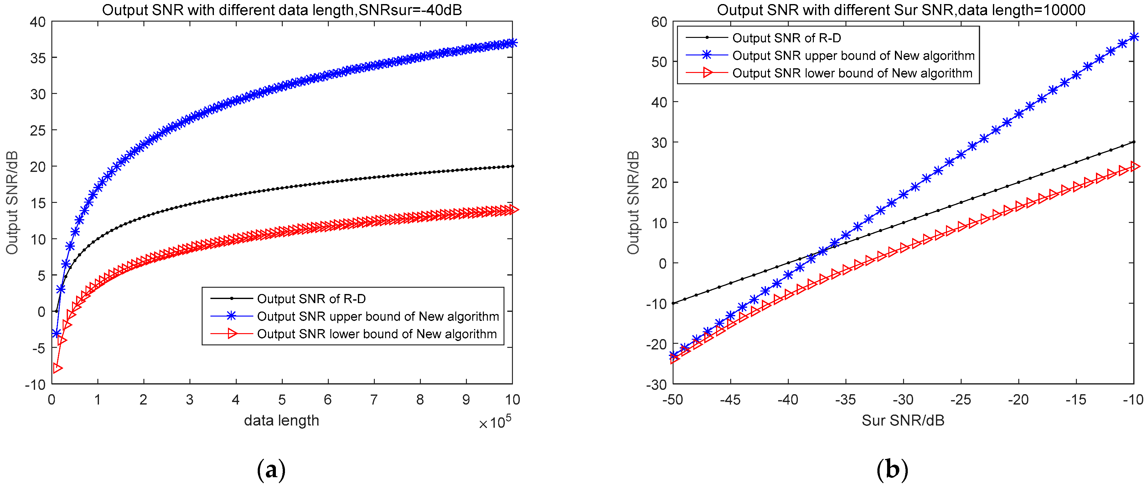
Figure 22 presents a comparison of the output SNR between two algorithms. When the cross phase of the differential signal is completely correlated, the output SNR of the algorithm obtains the minimum value, that is, the theoretical lower bound in Figure 22. When the cross term of the differential signal is completely uncorrelated, the output SNR of the algorithm reaches the maximum value, that is, the theoretical upper bound in Figure 22. As can be seen from Figure 22, the theoretical lower bound of the output SNR of the algorithm in this paper is lower than that of the traditional R-D algorithm, but the theoretical upper bound is much higher than that of the traditional algorithm. However, the cross item is the corresponding point multiplication of the reference signal and noise with different delays. The cross term cannot be completely correlated, and there must be a certain phase difference. Therefore, the lower bound of the output SNR for this algorithm cannot be achieved through practical processing.

4.2. The Influence of the Reference Channel SNR on the Performance of the Algorithms

When considering the SNR of the reference channel, from Equation (25), the output SNR of R-D algorithm is as follows:

$$G_r=\frac{{\left|A_{ref}\right|}^2{\left|a_1\right|}^2{N}^2}{\left({\left|A_{ref}\right|}^2+{\left|a_1\right|}^2+1\right)N}=\frac{{\left|a_1\right|}^2}{1+{\left|a_1\right|}^2/{\left|A_{ref}\right|}^2+1/{\left|A_{ref}\right|}^2}N$$

(50)

For differential operations in this paper, after compensating the time delay and frequency offset in Equation (13):

$$\begin{array}{l}W[\lambda ,f]={\displaystyle \sum _{l=1}^{N-1}{\displaystyle \sum _{k=1}^{N}R(l,k)\exp \left[-j2\pi (f\frac{l}{f_s}+\lambda k)\right]}}\\ ={\displaystyle \sum _{l=1}^{N-1}{\displaystyle \sum _{k=1}^N\left\{\begin{array}{c}{\left|A_{ref}^{}\right|}^2{\left|a_1^{}\right|}^2{e}^{j2\pi (f_{d1}-f)\frac{l}{f_s}}{P}_l(k)P_l^{*}(k)e^{-j2\pi ({\lambda }_1+\lambda )k}\hfill \\ +Z_{r,r}^{*}(l,k)\cdot {\left|a_1^{}\right|}^2{e}^{j2\pi (f_{d1}-f)\frac{l}{f_s}}{P}_l(k)e^{-j2\pi ({\lambda }_1+\lambda )k}\hfill \\ +Z_{r,r}^{*}(l,k)\cdot FFT\left(\begin{array}{l}{a}_1^{*}{z}_{sur}[n]d^{*}[n-{\lambda }_1-l]e^{-j2\pi f_{d1}(\frac{n}{f_s}-\frac{l}{f_s})}\\ +a_1{z}_{sur}^{*}[n-l]d[n-{\lambda }_1]e^{j2\pi f_{d1}(\frac{n}{f_s})}\\ +z_{sur}^{*}[n-l]z_{sur}[n]\end{array}\right)e^{j2\pi f\frac{l}{f_s}}{e}^{-j2\pi \lambda k}\hfill \\ +{\left|A_{ref}^{}\right|}^2{P}_l^{*}(k)\cdot FFT\left(\begin{array}{l}{a}_1^{*}{z}_{sur}[n]d^{*}[n-{\lambda }_1-l]e^{-j2\pi f_{d1}(\frac{n}{f_s}-\frac{l}{f_s})}\\ +a_1{z}_{sur}^{*}[n-l]d[n-{\lambda }_1]e^{j2\pi f_{d1}(\frac{n}{f_s})}\\ +z_{sur}^{*}[n-l]z_{sur}[n]\end{array}\right)e^{j2\pi f\frac{l}{f_s}}{e}^{-j2\pi \lambda k}\hfill \end{array}\right\}}}\end{array}$$

(51)

when $\lambda =-{\lambda }_1$ and $f=f_{d1}$, the peak appears at the location of target 1:

$$\begin{array}{ll}{\left|\eta [{\lambda }_1,f_{d1}]\right|}^2\approx & \left|\begin{array}{l}{\eta }_{sr}{[{\lambda }_1,f_{d1}]}^2+{\eta }_{2,1}{[{\lambda }_1,f_{d1}]}^2+{\eta }_{2,2}{[{\lambda }_1,f_{d1}]}^2+{\eta }_{2,3}{[{\lambda }_1,f_{d1}]}^2+{\eta }_{3,1}{[{\lambda }_1,f_{d1}]}^2\\ +{\eta }_{3,2}{[{\lambda }_1,f_{d1}]}^2+{\eta }_{3,3}{[{\lambda }_1,f_{d1}]}^2+{\eta }_{3,4}{[{\lambda }_1,f_{d1}]}^2+{\eta }_{3,5}{[{\lambda }_1,f_{d1}]}^2+{\eta }_{3,6}{[{\lambda }_1,f_{d1}]}^2\\ +{\eta }_{3,7}{[{\lambda }_1,f_{d1}]}^2+{\eta }_{3,8}{[{\lambda }_1,f_{d1}]}^2+{\eta }_{3,9}{[{\lambda }_1,f_{d1}]}^2+{\eta }_{3,10}{[{\lambda }_1,f_{d1}]}^2+{\eta }_{3,11}{[{\lambda }_1,f_{d1}]}^2\\ +{\eta }_{3,12}{[{\lambda }_1,f_{d1}]}^2+{\eta }_{4,1}{[{\lambda }_1,f_{d1}]}^2+{\eta }_{4,2}{[{\lambda }_1,f_{d1}]}^2+{\eta }_{4,3}{[{\lambda }_1,f_{d1}]}^2+{\eta }_{4,4}{[{\lambda }_1,f_{d1}]}^2\end{array}\right|\end{array}$$

(52)

$${\left|{\eta }_{sr}[{\lambda }_1,f_{d1}]\right|}^2={\displaystyle \sum _{l=1}^{N-1}{\displaystyle \sum _{k=1}^N\left\{{\left|A_{ref}\right|}^2{\left|a_1\right|}^2{P}_l(k)P_l^{*}(k)\right\}}}={\left|A_{ref}\right|}^4{\left|a_1\right|}^4{\left({\displaystyle \sum _{l=1}^{N-1}(N-l)}\right)}^2$$

(53)

The signal shown in Equation (53) has no phase difference after compensation and is a sequence of real numbers. Therefore, its coherent accumulation gain can be seen as a coherent accumulation of signal with data length ${\displaystyle \sum _{l=1}^{N-1}(N-l)}$.

$${\left|{\eta }_{3,9}[{\lambda }_1,f_{d1}]\right|}^2={\left\{{\displaystyle \sum _{l=1}^{N-1}{\displaystyle \sum _{k=1}^N\left\{z_{ref}[n]z_{ref}^{*}[n-l]FFT\left(z_{sur}^{*}[n-l]z_{sur}[n]\right)e^{j2\pi f_{d1}\frac{l}{f_s}}{e}^{-j2\pi {\lambda }_{1}k}\right\}}}\right\}}^2$$

(54)

$${\left|{\eta }_{2,3}[{\lambda }_1,f_{d1}]\right|}^2={\left\{{\displaystyle \sum _{l=1}^{N-1}{\displaystyle \sum _{k=1}^N\left\{z_{ref}[n]z_{ref}^{*}[n-l]{\left|a_1\right|}^2{P}_l(k)\right\}}}\right\}}^2$$

(55)

$${\left|{\eta }_{3,8}[{\lambda }_1,f_{d1}]\right|}^2={\left\{{\displaystyle \sum _{l=1}^{N-1}{\displaystyle \sum _{k=1}^N\left\{z_{ref}[n]z_{ref}^{*}[n-l]FFT\left(a_1{z}_{sur}^{*}[n-l]d[n-{\lambda }_1]e^{j2\pi f_{d1}(\frac{n}{f_s})}\right)e^{j2\pi f_{d1}\frac{l}{f_s}}{e}^{-j2\pi {\lambda }_{1}k}\right\}}}\right\}}^2$$

(56)

$${\left|{\eta }_{4,3}[{\lambda }_1,f_{d1}]\right|}^2={\left\{{\displaystyle \sum _{l=1}^{N-1}{\displaystyle \sum _{k=1}^N\left\{{\left|A_{ref}\right|}^2{P}_l^{*}(k)\cdot FFT\left(z_{sur}^{*}[n-l]z_{sur}[n]\right)e^{j2\pi f_{d1}\frac{l}{f_s}}{e}^{-j2\pi {\lambda }_{1}k}\right\}}}\right\}}^2$$

(57)

Under different difference orders l, the signals in Equation (54) are approximately uncorrelated. However, the signals in Equations (55)–(57) all contain completely uncorrelated items and incompletely correlated items, which mean that the correlation are relatively weak. Therefore, they are also considered to be approximately uncorrelated. Therefore, its accumulated gain can be approximately regarded as the incoherent accumulated gain of a signal with length ${\displaystyle \sum _{l=1}^{N-1}(N-l)}$. The accumulated gain is shown in the following Equations (58)–(61):

$${\left|{\eta }_{3,9}[{\lambda }_1,f_{d1}]\right|}^2\approx {\displaystyle \sum _{l=1}^{N-1}(N-l)}$$

(58)

$${\left|{\eta }_{2,3}[{\lambda }_1,f_{d1}]\right|}^2\approx {\left|a_1\right|}^4{\displaystyle \sum _{l=1}^{N-1}(N-l)}$$

(59)

$${\left|{\eta }_{3,8}[{\lambda }_1,f_{d1}]\right|}^2\approx {\left|a_1\right|}^2{\displaystyle \sum _{l=1}^{N-1}(N-l)}$$

(60)

$${\left|{\eta }_{4,3}[{\lambda }_1,f_{d1}]\right|}^2\approx {\left|A_{ref}\right|}^4{\displaystyle \sum _{l=1}^{N-1}(N-l)}$$

(61)

$${\left|{\eta }_{2,1}[{\lambda }_1,f_{d1}]\right|}^2={\left\{{\displaystyle \sum _{l=1}^{N-1}{\displaystyle \sum _{k=1}^N\left\{A_{ref}^{*}{z}_{ref}[n]d^{*}[n-l]{\left|a_1\right|}^2{P}_l(k)\right\}}}\right\}}^2$$

(62)

$${\left|{\eta }_{2,2}[{\lambda }_1,f_{d1}]\right|}^2={\left\{{\displaystyle \sum _{l=1}^{N-1}{\displaystyle \sum _{k=1}^N\left\{A_{ref}d[n]\cdot z_{ref}^{*}[n-l]{\left|a_1\right|}^2{P}_l(k)\right\}}}\right\}}^2$$

(63)

$${\left|{\eta }_{3,1}[{\lambda }_1,f_{d1}]\right|}^2={\left\{{\displaystyle \sum _{l=1}^{N-1}{\displaystyle \sum _{k=1}^N\left\{A_{ref}^{*}{z}_{ref}[n]d^{*}[n-l]FFT\left(a_1^{*}{z}_{sur}[n]d^{*}[n-{\lambda }_1-l]e^{-j2\pi f_{d1}(\frac{n}{f_s}-\frac{l}{f_s})}\right)e^{j2\pi f_{d1}\frac{l}{f_s}}{e}^{-j2\pi {\lambda }_{1}k}\right\}}}\right\}}^2$$

(64)

$${\left|{\eta }_{3,2}[{\lambda }_1,f_{d1}]\right|}^2={\left\{{\displaystyle \sum _{l=1}^{N-1}{\displaystyle \sum _{k=1}^N\left\{A_{ref}^{*}{z}_{ref}[n]d^{*}[n-l]FFT\left(a_1{z}_{sur}^{*}[n-l]d[n-{\lambda }_1]e^{j2\pi f_{d1}(\frac{n}{f_s})}\right)e^{j2\pi f_{d1}\frac{l}{f_s}}{e}^{-j2\pi {\lambda }_{1}k}\right\}}}\right\}}^2$$

(65)

$${\left|{\eta }_{3,3}[{\lambda }_1,f_{d1}]\right|}^2={\left\{{\displaystyle \sum _{l=1}^{N-1}{\displaystyle \sum _{k=1}^N\left\{A_{ref}^{*}{z}_{ref}[n]d^{*}[n-l]FFT\left(z_{sur}^{*}[n-l]z_{sur}[n]\right)e^{j2\pi f_{d1}\frac{l}{f_s}}{e}^{-j2\pi {\lambda }_{1}k}\right\}}}\right\}}^2$$

(66)

$${\left|{\eta }_{3,4}[{\lambda }_1,f_{d1}]\right|}^2={\left\{{\displaystyle \sum _{l=1}^{N-1}{\displaystyle \sum _{k=1}^N\left\{A_{ref}d[n]\cdot z_{ref}^{*}[n-l]FFT\left(a_1^{*}{z}_{sur}[n]d^{*}[n-{\lambda }_1-l]e^{-j2\pi f_{d1}(\frac{n}{f_s}-\frac{l}{f_s})}\right)e^{j2\pi f_{d1}\frac{l}{f_s}}{e}^{-j2\pi {\lambda }_{1}k}\right\}}}\right\}}^2$$

(67)

$${\left|{\eta }_{3,5}[{\lambda }_1,f_{d1}]\right|}^2={\left\{{\displaystyle \sum _{l=1}^{N-1}{\displaystyle \sum _{k=1}^N\left\{A_{ref}d[n]\cdot z_{ref}^{*}[n-l]FFT\left(a_1{z}_{sur}^{*}[n-l]d[n-{\lambda }_1]e^{j2\pi f_{d1}(\frac{n}{f_s})}\right)e^{j2\pi f_{d1}\frac{l}{f_s}}{e}^{-j2\pi {\lambda }_{1}k}\right\}}}\right\}}^2$$

(68)

$${\left|{\eta }_{3,6}[{\lambda }_1,f_{d1}]\right|}^2={\left\{{\displaystyle \sum _{l=1}^{N-1}{\displaystyle \sum _{k=1}^N\left\{A_{ref}d[n]\cdot z_{ref}^{*}[n-l]FFT\left(z_{sur}^{*}[n-l]z_{sur}[n]\right)e^{j2\pi f_{d1}\frac{l}{f_s}}{e}^{-j2\pi {\lambda }_{1}k}\right\}}}\right\}}^2$$

(69)

$${\left|{\eta }_{3,7}[{\lambda }_1,f_{d1}]\right|}^2={\left\{{\displaystyle \sum _{l=1}^{N-1}{\displaystyle \sum _{k=1}^N\left\{z_{ref}[n]z_{ref}^{*}[n-l]FFT\left(a_1^{*}{z}_{sur}[n]d^{*}[n-{\lambda }_1-l]e^{-j2\pi f_{d1}(\frac{n}{f_s}-\frac{l}{f_s})}\right)e^{j2\pi f_{d1}\frac{l}{f_s}}{e}^{-j2\pi {\lambda }_{1}k}\right\}}}\right\}}^2$$

(70)

$${\left|{\eta }_{4,1}[{\lambda }_1,f_{d1}]\right|}^2={\left\{{\displaystyle \sum _{l=1}^{N-1}{\displaystyle \sum _{k=1}^N\left\{{\left|A_{ref}\right|}^2{P}_l^{*}(k)\cdot FFT\left(a_1^{*}{z}_{sur}[n]d^{*}[n-{\lambda }_1-l]e^{-j2\pi f_{d1}(\frac{n}{f_s}-\frac{l}{f_s})}\right)e^{j2\pi f_{d1}\frac{l}{f_s}}{e}^{-j2\pi {\lambda }_{1}k}\right\}}}\right\}}^2$$

(71)

$${\left|{\eta }_{4,2}[{\lambda }_1,f_{d1}]\right|}^2={\left\{{\displaystyle \sum _{l=1}^{N-1}{\displaystyle \sum _{k=1}^N\left\{{\left|A_{ref}\right|}^2{P}_l^{*}(k)\cdot FFT\left(a_1{z}_{sur}^{*}[n-l]d[n-{\lambda }_1]e^{j2\pi f_{d1}(\frac{n}{f_s})}\right)e^{j2\pi f_{d1}\frac{l}{f_s}}{e}^{-j2\pi {\lambda }_{1}k}\right\}}}\right\}}^2$$

(72)

The signal in Formulas (62)–(72) includes both completely related items and incompletely related items. In the same differential order, due to the phase difference of the signal itself, only incoherent accumulation can be achieved. Meanwhile, it is possible that the correlation of each signal changes from approximately uncorrelated to completely correlated under different differential orders. Therefore, when the signals are completely correlated, the algorithm in this paper obtains the theoretical lower bound of the accumulated gain, and each accumulated gain is shown in the following formulas:

$${\left|{\eta }_{2,1}[{\lambda }_1,f_{d1}]\right|}^2\approx {\left|A_{ref}\right|}^2{\left|a_1\right|}^4(N-2){\displaystyle \sum _{l=1}^{N-1}(N-l)}$$

(73)

$${\left|{\eta }_{2,2}[{\lambda }_1,f_{d1}]\right|}^2\approx {\left|A_{ref}\right|}^2{\left|a_1\right|}^4(N-2){\displaystyle \sum _{l=1}^{N-1}(N-l)}$$

(74)

$${\left|{\eta }_{3,1}[{\lambda }_1,f_{d1}]\right|}^2\approx {\left|A_{ref}\right|}^2{\left|a_m\right|}^2(N-2){\displaystyle \sum _{l=1}^{N-1}(N-l)}$$

(75)

$${\left|{\eta }_{3,2}[{\lambda }_1,f_{d1}]\right|}^2\approx {\left|A_{ref}\right|}^2{\left|a_1\right|}^2(N-2){\displaystyle \sum _{l=1}^{N-1}(N-l)}$$

(76)

$${\left|{\eta }_{3,3}[{\lambda }_1,f_{d1}]\right|}^2\approx {\left|A_{ref}\right|}^2(N-2){\displaystyle \sum _{l=1}^{N-1}(N-l)}$$

(77)

$${\left|{\eta }_{3,4}[{\lambda }_1,f_{d1}]\right|}^2\approx {\left|A_{ref}\right|}^2{\left|a_1\right|}^2(N-2){\displaystyle \sum _{l=1}^{N-1}(N-l)}$$

(78)

$${\left|{\eta }_{3,5}[{\lambda }_1,f_{d1}]\right|}^2\approx {\left|A_{ref}\right|}^2{\left|a_1\right|}^2(N-2){\displaystyle \sum _{l=1}^{N-1}(N-l)}$$

(79)

$${\left|{\eta }_{3,6}[{\lambda }_1,f_{d1}]\right|}^2\approx {\left|A_{ref}\right|}^2(N-2){\displaystyle \sum _{l=1}^{N-1}(N-l)}$$

(80)

$${\left|{\eta }_{3,7}[{\lambda }_1,f_{d1}]\right|}^2\approx {\left|a_1\right|}^2(N-2){\displaystyle \sum _{l=1}^{N-1}(N-l)}$$

(81)

$${\left|{\eta }_{4,1}[{\lambda }_1,f_{d1}]\right|}^2\approx {\left|A_{ref}\right|}^4{\left|a_1\right|}^2(N-2){\displaystyle \sum _{l=1}^{N-1}(N-l)}$$

(82)

$${\left|{\eta }_{4,2}[{\lambda }_1,f_{d1}]\right|}^2\approx {\left|A_{ref}\right|}^4{\left|a_1\right|}^2(N-2){\displaystyle \sum _{l=1}^{N-1}(N-l)}$$

(83)

When the signals are non-correlated, the algorithm in this paper obtains the theoretical upper bound of the accumulated gain, and accumulated gains are shown in the following formulas:

$${\left|{\eta }_{2,1}[{\lambda }_1,f_{d1}]\right|}^2\approx {\left|A_{ref}\right|}^2{\left|a_1\right|}^4{\displaystyle \sum _{l=1}^{N-1}(N-l)}$$

(84)

$${\left|{\eta }_{2,2}[{\lambda }_1,f_{d1}]\right|}^2\approx {\left|A_{ref}\right|}^2{\left|a_1\right|}^4{\displaystyle \sum _{l=1}^{N-1}(N-l)}$$

(85)

$${\left|{\eta }_{3,1}[{\lambda }_1,f_{d1}]\right|}^2\approx {\left|A_{ref}\right|}^2{\left|a_m\right|}^2{\displaystyle \sum _{l=1}^{N-1}(N-l)}$$

(86)

$${\left|{\eta }_{3,2}[{\lambda }_1,f_{d1}]\right|}^2\approx {\left|A_{ref}\right|}^2{\left|a_1\right|}^2{\displaystyle \sum _{l=1}^{N-1}(N-l)}$$

(87)

$${\left|{\eta }_{3,3}[{\lambda }_1,f_{d1}]\right|}^2\approx {\left|A_{ref}\right|}^2{\displaystyle \sum _{l=1}^{N-1}(N-l)}$$

(88)

$${\left|{\eta }_{3,4}[{\lambda }_1,f_{d1}]\right|}^2\approx {\left|A_{ref}\right|}^2{\left|a_1\right|}^2{\displaystyle \sum _{l=1}^{N-1}(N-l)}$$

(89)

$${\left|{\eta }_{3,5}[{\lambda }_1,f_{d1}]\right|}^2\approx {\left|A_{ref}\right|}^2{\left|a_1\right|}^2{\displaystyle \sum _{l=1}^{N-1}(N-l)}$$

(90)

$${\left|{\eta }_{3,6}[{\lambda }_1,f_{d1}]\right|}^2\approx {\left|A_{ref}\right|}^2{\displaystyle \sum _{l=1}^{N-1}(N-l)}$$

(91)

$${\left|{\eta }_{3,7}[{\lambda }_1,f_{d1}]\right|}^2\approx {\left|a_1\right|}^2{\displaystyle \sum _{l=1}^{N-1}(N-l)}$$

(92)

$${\left|{\eta }_{4,1}[{\lambda }_1,f_{d1}]\right|}^2\approx {\left|A_{ref}\right|}^4{\left|a_1\right|}^2{\displaystyle \sum _{l=1}^{N-1}(N-l)}$$

(93)

$${\left|{\eta }_{4,2}[{\lambda }_1,f_{d1}]\right|}^2\approx {\left|A_{ref}\right|}^4{\left|a_1\right|}^2{\displaystyle \sum _{l=1}^{N-1}(N-l)}$$

(94)

The theoretical upper bound output SNR in this paper is as follows:

$$\begin{array}{l}{G}_{upper}=\frac{{\left|A_{ref}\right|}^4{\left|a_1\right|}^4{\left\{{\displaystyle \sum _{l=1}^{N-1}} (N-l)\right\}}^2}{\left(2{\left|A_{ref}\right|}^4{\left|a_1\right|}^2+{\left|A_{ref}\right|}^4+2{\left|A_{ref}\right|}^2{\left|a_1\right|}^4+4{\left|A_{ref}\right|}^2{\left|a_1\right|}^2+2{\left|A_{ref}\right|}^2+{\left|a_1\right|}^4+2{\left|a_1\right|}^2+1\right){\displaystyle \sum _{l=1}^{N-1}} (N-l)}\hfill \\ \hspace{1em}\hspace{0.17em}\hspace{1em}=\frac{A_{ref}^4{a}_1^4}{\left(2{\left|A_{ref}\right|}^4{\left|a_1\right|}^2+{\left|A_{ref}\right|}^4+2{\left|A_{ref}\right|}^2{\left|a_1\right|}^4+4{\left|A_{ref}\right|}^2{\left|a_1\right|}^2+2{\left|A_{ref}\right|}^2+{\left|a_1\right|}^4+2{\left|a_1\right|}^2+1\right)}{\displaystyle \sum _{l=1}^{N-1}} (N-l)\end{array}$$

(95)

The theoretical lower bound output SNR in this paper is as follows:

$$G_{lower}=\frac{{\left|A_{ref}\right|}^4{\left|a_1\right|}^4{\left({\displaystyle \sum _{l=1}^{N-1}l}\right)}^2}{\left\{\begin{array}{l}(N-2)\left\{2{\left|A_{ref}\right|}^4{\left|a_1\right|}^2+2{\left|A_{ref}\right|}^2{\left|a_1\right|}^4+4{\left|A_{ref}\right|}^2{\left|a_1\right|}^2+2{\left|A_{ref}\right|}^2+{\left|a_1\right|}^2\right\}{\displaystyle \sum _{l=1}^{N-1}(N-l)}\\ +({\left|a_1\right|}^4+{\left|A_{ref}\right|}^4+{\left|a_1\right|}^2+1){\displaystyle \sum _{l=1}^{N-1}(N-l)}\end{array}\right\}}$$

(96)

When the SNR of the reference channel tends to infinity, the derivation in Equations (95) and (96) is consistent with that in Equations (48) and (49).

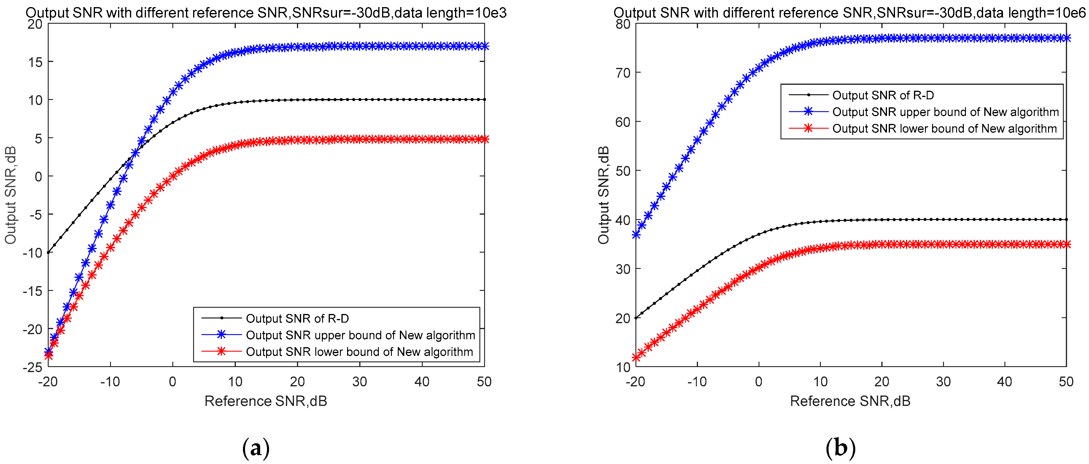
Figure 23 shows the output SNR under different reference SNR. It can be seen from Figure 23 that the algorithm in this paper is more greatly affected by the SNR of the reference channel. However, when the SNR is relatively high, the estimation performance is better than that attained with traditional R-D processing. In the detection of the passive radar, the reference antenna generally points directly to the direction of the emitter, so that the SNR of the reference channel is generally higher than 0 dB. Therefore, in practical applications, the estimation performance of this algorithm is better than that of the traditional R-D algorithm.

From the above analysis, the performance of this algorithm is higher than that of the traditional R-D algorithm. With the increase of SNR of target echo channel and accumulation time, it increases continuously. However, the detection performance of the algorithm in this paper is greatly affected under lower reference channel SNR.

5. Conclusions

In this paper, we proposed a novel cross-correlation algorithm for the passive radar, which breaks through the optimal limits of the traditional cross-correlation algorithm under the condition of a high reference channel SNR. The algorithm uses the differential to convert a single signal received by the echo antenna into multi-channel signals and then uses the differential multi-channel reference signal to eliminate the phase influence of the signal itself in the target echo. This can achieve the twice coherent accumulation of the target echo. At the same time, due to the phase and correlation difference of the noise and interference signals, only twice the incoherent accumulation can be realized. In traditional R-D processing, the target echo achieves one coherent accumulation and the target and interference also carry out one incoherent accumulation. Therefore, compared with the traditional algorithm, our algorithm can greatly improve the target detection performance. Meanwhile, the target detection results of the simulation data and measured data are basically consistent with the theoretical derivation results presented in this paper. The target detection performance of this algorithm is much better than that attained with traditional R-D processing, and the output SNR of our algorithm can be improved faster with an increase in the accumulation time.

At the same time, it should be noted that the algorithm presented in this paper requires a large amount of computation, and parallel processing and faster two-dimensional Fourier transform may need to be introduced. This is left for future work.

References

- Zhu, Y.; Liang, S.; Gong, M.; Yan, J. Decomposed POMDP Optimization-Based Sensor Management for Multi-Target Tracking in Passive Multi-Sensor Systems. IEEE Sens. J. 2022, 22, 3565–3578. [Google Scholar] [CrossRef]
- You, H.; Jian, G.; Meng, X. Radar Target Detection and CFAR Processing; Tsinghua University Press: Beijing, China, 2011. [Google Scholar]
- Xiong, J.; Hong, H.; Zhang, H.; Wang, N.; Chu, H.; Zhu, X. Multitarget Respiration Detection With Adaptive Digital Beamforming Technique Based on SIMO Radar. IEEE Trans. Microw. Theory Tech. 2020, 68, 4814–4824. [Google Scholar] [CrossRef]
- Yuan, S.; Fan, W.; Xu, L. Tow-Ship Interference Suppression Based on Blind Source Separation for Passive Sonar. In Proceedings of the Third International Symposium on Parallel Architectures, Liaoning, China, 18–20 December 2010. [Google Scholar]
- Melvin, W.L. Space-Time Adaptive Processing for Radar. Acad. Press Libr. Signal Process. 2014, 2, 595–665. [Google Scholar]
- Colone, F.; O’Hagan, D.W.; Lombardo, P.; Baker, C.J. A Multistage Processing Algorithm for Disturbance Removal and Target Detection in Passive Bistatic Radar. IEEE Trans. Aerosp. Electron. Syst. 2009, 45, 698–722. [Google Scholar] [CrossRef]
- Griffin, D.W.; Lim, J.S. Multiband excitation vocoder. IEEE Trans. Acoust. Speech Signal Process. 1988, 36, 1223–1235. [Google Scholar] [CrossRef] [Green Version]
- Ma, X.; Yuan, J. Simulation Analysis for MTD Detectability Improvement Using the Discrete Wavelet Transform (DWT). J. Signal Process. 2001, 17, 148–151. [Google Scholar]
- Howland, P.E.; Maksimiuk, D.; Reitsma, G. FM radio based bistatic radar. IEE Proc.—Radar Sonar Navig. 2005, 152, 107–115. [Google Scholar] [CrossRef] [Green Version]
- Coleman, C.; Yardley, H. Passive bistatic radar based on target illuminations by digital audio broadcasting. IET Radar Sonar Navig. 2008, 2, 366–375. [Google Scholar] [CrossRef]
- Park, G.H.; Seo, Y.K.; Kim, H.N. Range-Doppler Domain-Based DOA Estimation Method for FM-Band Passive Bistatic Radar. IEEE Access 2020, 8, 56880–56891. [Google Scholar] [CrossRef]
- Park, G.H.; Kim, H.N. Convolutional Neural Network-based Target Detection Method for Passive Bistatic Radar using FM Broadcasting Signals. J. Inst. Electron. Inf. Eng. 2020, 57, 70–78. [Google Scholar]
- Griffiths, H.D.; Long, N.R. Television-based bistatic radar. IEE Proc. F Commun. Radar Signal Process. 1986, 133, 649–657. [Google Scholar] [CrossRef]
- Poullin, D. Passive detection using digital broadcasters (DAB, DVB) with COFDM modulation. IEE Proc.—Radar Sonar Navig. 2005, 152, 143–152. [Google Scholar] [CrossRef]
- Wang, H.; Wang, J.; Zhong, L. Mismatched filter for analogue TV-based passive bistatic radar. IET Radar Sonar Navig. 2011, 5, 573–581. [Google Scholar] [CrossRef]
- Tao, R.; Wu, H.; Shan, T. Direct-path suppression by spatial filtering in digital television terrestrial broadcasting-based passive radar. IET Radar Sonar Navig. 2010, 4, 791–805. [Google Scholar] [CrossRef]
- Tan, D.; Sun, H.; Lu, Y.; Lesturgie, M.; Chan, H. Passive radar using Global System for Mobile communication signal: Theory, implementation and measurements. IEE Proc.—Radar Sonar Navig. 2005, 152, 116–123. [Google Scholar] [CrossRef]
- Guo, H.; Woodbridge, K.; Baker, C.J. Evaluation of WIFI beacon transmissions for wireless based passive radar. In Proceedings of the 2008 IEEE Radar Conference, Rome, Italy, 26–30 May 2008; pp. 1–6. [Google Scholar]
- Wang, H.; Wang, J.; Li, H. Target detection using CDMA based passive bistatic radar. Syst. Eng. Electron. Technol. (Engl. Version) 2012, 23, 858–865. [Google Scholar] [CrossRef]
- Salah, A.A.; Raja Abdullah, R.S.; Ismail, A.; Hashim, F.; Abdul Aziz, N.H. Experimental study of LTE signals as illuminators of opportunity for passive bistatic radar applications. Electron. Lett. 2014, 50, 545–547. [Google Scholar] [CrossRef]
- Maussang, F.; Garello, R.; Soulat, F.; Desjonqueres, J.D.; Pourthie, N. GPS passive bistatic radar system in oceanic environment: Detection performance estimation. In Proceedings of the OCEANS 2011 IEEE-Spain, Santander, Spain, 6–9 June 2011. [Google Scholar]
- Chow, Y.P.; Trinkle, M. Experimental Results Investigating the Feasibility of GPS Bistatic Radar for Target Detection and Estimation. In Proceedings of the 24th International Technical Meeting of the Satellite Division of The Institute of Navigation (ION GNSS 2011), Portland, OR, USA, 20–23 September 2011. [Google Scholar]
- Huang, P.; Liao, G.; Yang, Z.; Shu, Y.; Du, W. Approach for space-based radar manoeuvring target detection and high-order motion parameter estimation. IET Radar Sonar Navig. 2015, 9, 732–741. [Google Scholar] [CrossRef]
- Carlson, B.D.; Evans, E.D.; Wilson, S.L. Errata: Search radar detection and track with the Hough transform. IEEE Trans. Aerosp. Electron. Syst. 2003, 30, 109–115. [Google Scholar] [CrossRef]
- Boers, Y.; Mandal, P.K. Optimal Particle-Filter-Based Detector. IEEE Signal Process. Lett. 2019, 26, 435–439. [Google Scholar] [CrossRef] [Green Version]
- Kim, D.Y.; Ristic, B.; Guan, R.; Rosenberg, L. A Bernoulli Track-Before-Detect Filter for Interacting Targets in Maritime Radar. IEEE Trans. Aerosp. Electron. Syst. 2021, 57, 1981–1991. [Google Scholar] [CrossRef]
- Quan, N.V.; Markelov, O.A.; Veremyev, V.I. Passive Bistatic Radar Monitoring with GPS Satellites as Transmitters of Opportunity. In Proceedings of the 2021 IEEE Conference of Russian Young Researchers in Electrical and Electronic Engineering (ElConRus), St. Petersburg, Moscow, Russia, 26–29 January 2021. [Google Scholar]
- Chen, X.; Guan, J.; Liu, N.; He, Y. Maneuvering Target Detection via Radon-Fractional Fourier Transform-Based Long-Time Coherent Integration. IEEE Trans. Signal Process. 2014, 62, 939–953. [Google Scholar] [CrossRef]
- Hou, L.; Song, H.; Zheng, M.; Wang, W. Fast moving target imaging and motion parameters estimation based on Radon transform and bi-directional approach. IET Radar Sonar Navig. 2016, 10, 1013–1023. [Google Scholar] [CrossRef]
- Gao, Z.; Tao, R. Calculation and performance analysis of coherent integration gain of passive radar. J. Electron. 2008, 36, 1227–1230. [Google Scholar]
Figure 1.
Passive radar system schematic.
Figure 2.
Integration results with traditional R-D processing: N = 104 (a) Doppler dimension; (b) Range dimension.
Figure 3.
Integration results with the proposed method: N = 104 (a) Doppler dimension; (b) Range dimension.
Figure 4.
Difference between the target peak and the average noise platform (N = 104).
Figure 5.
Precision of target detection with different noise power values (N = 104).
Figure 6.
Figure 7.
Comparison of ROC curve without reference noise (N = 104).
Figure 8.
Integration results with traditional R-D processing: ; (a) Doppler dimension; (b) Range dimension.
Figure 9.
Integration results with the proposed method: ; (a) Doppler dimension; (b) Range dimension.
Figure 10.
Figure 11.
Precision of target detection with different noise power values (N = 104): reference SNR = 0 dB.
Figure 12.
Figure 13.
Precision of target detection with different noise power values (N = 104): reference SNR = −10 dB.
Figure 14.
Comparison of ROC curve with SNRref = 10 dB (N = 104).
Figure 15.
Comparison of ROC curve with SNRref = −5 dB (N = 104).
Figure 16.
Integration results with traditional R-D processing for the audio signal: N = 105; (a) Doppler dimension; (b) Range dimension.
Figure 17.
Integration results obtained with traditional R-D processing for the audio signal: ; (a) Doppler dimension; (b) Range dimension.
Figure 18.
Integration results obtained with the proposed method for the audio signal: N = 105; (a) Doppler dimension; (b) Range dimension.
Figure 19.
Integration results obtained with proposed method for the audio signal: ; (a) Doppler dimension; (b) Range dimension.
Figure 20.
Integration results with traditional R-D processing for the FM signal: (a) ; (b) .
Figure 21.
Integration results obtained with the proposed method for the FM signal: (a) ; (b) .
Figure 22.
Comparison of the output SNR between the two algorithms: (a) comparison under different signal lengths: SNRsur = −40 dB; (b) comparison under different SNRsur: N = 104.
Figure 23.
Output SNR under different reference SNR (SNRsur = −30 dB: (a) N = 104, (b) N = 106).