
Fast Target Localization in FMCW-MIMO Radar with Low SNR and Snapshot via Multi-DeepNet


1
School of Information and Communication Engineering, Hainan University, Haikou 570228, China
2
College of Information Engineering, Hainan Vocational University of Science and Technology, Haikou 571158, China
3
Department of Communication Engineering, Institute of Information Science Technology, Dalian Maritime University, Dalian 116026, China
*
Author to whom correspondence should be addressed.
Remote Sens. 2023, 15(1), 66; https://doi.org/10.3390/rs15010066
Submission received: 23 October 2022
/
Revised: 5 December 2022
/
Accepted: 16 December 2022
/
Published: 23 December 2022
(This article belongs to the Topic Advances in Array Signal Processing with Errors: Models, Algorithms and Applications)
Abstract
:Frequency modulated continuous wave (FMCW) multiple-input multiple-output (MIMO) radars are widely applied in target localization. However, during the process, the estimation accuracy decreases sharply without considerable signal-to-noise ratio (SNR) and sufficient snapshot number. It is therefore necessary to consider estimation schemes that are valid under low signal-to-noise ratio (SNR) and snapshot. In this paper, a fast target localization framework based on multiple deep neural networks named Multi-DeepNet is proposed. In the scheme, multiple interoperating deep networks are employed to achieve accurate target localization in harsh environments. Firstly, we designed a coarse estimate using deep learning to determine the interval where the angle is located. Then, multiple neural networks are designed to realize accurate estimation. After that, the range estimation is determined. Finally, angles and ranges are matched by comparing the Frobenius norm. Simulations and experiments are conducted to verify the efficiency and accuracy of the proposed framework.
1. Introduction
Frequency modulated continuous wave (FMCW) radar is widely used in civil fields, such as road vehicle monitoring and recording systems, car collision avoidance radars, traffic flow detectors and automatic driving systems, because of its easy implementation, simple structure, small size, light weight and low cost [1,2,3]. Researchers have also applied FMCW radar to micro-motion scenarios such as heartbeat detection and posture detection due to its excellent characteristics [4].
Recent studies have investigated multiple-input multiple-output (MIMO) FMCW radars, which pair the transmitter and receiver independently as virtual elements [5,6,7]. A large increase in array aperture is accompanied by an increase in data size. In addition, the received signal of the FMCW-MIMO radar contains DOA, speed and range information, which can be further used for target localization. In order to achieve this, the joint estimation of angle and range must be addressed. Since conventional algorithms, such as 2D-FFT, cannot obtain satisfactory performance due to the limitation of the Rayleigh criterion and the bandwidth of FMCW-MIMO radar, 2D-MUSIC is naturally applied to the joint angle and range estimation with the FMCW-MIMO radar [7,8]. In [9], J. Lee proposed a joint angle, speed and range estimation algorithm, where the 2D- MUSIC algorithm is applied to estimate both DOA and speed of the target. After that, a matched filter with the estimated angle and Doppler frequency as well as FFT operation is provided to estimate the range of the target. To further improve the performance, reference [10] proposed a gridless algorithm for joint DOA and range estimation. However, the estimation time required for 2D-MUSIC runs counter to the real-time requirements for radars today [11]. To enhance the speed of the algorithm, the feasible sparse spectrum fitting (SpSF) algorithm for FDA-MIMO radar is proposed in [12]. In addition, in [13], a linear predictive-orthogonal propagator method (LP-OPM) based on forward–backward spatial smoothing (SS) is proposed for target localization. The DOA and range are estimated separately by the SS-LP-OPM algorithm, and then the parameters are matched by the least squares (LS) method. However when the SNR and snapshot are low, the above algorithm has large error, and the running time could be improved. Afterwards, two fast methods based on PARFAC decomposition were proposed in [14,15], but their performance is more general in the case of low snapshots and SNR.
Over the past few years, deep learning (DL) and machine learning (ML) have become increasingly popular research topics. Additionally, data-driven algorithms have been widely used in DOA estimation [16,17,18,19,20,21,22] with some excellent results. In [16,17], DOA estimation methods combining DL and MUSIC algorithm are proposed to improve estimation performance significantly over ordinary MUSIC algorithms. With low SNR, the DL-based DOA estimation algorithm can achieve better estimation performance than conventional algorithms [18]. In the non-ideal situation with some types of noise and defects, the DL-based DOA estimation algorithm [19] is more adaptable than other algorithms. As with the fast DOA estimation algorithm proposed in [20], DL-based DOA estimation algorithms often offer considerable runtime advantages as well. Furthermore, the DL-based algorithm proposed in [21] achieves fast and high-accuracy DOA estimation. Even though all of these DL-based algorithms are considered to be faster or better than traditional algorithms, they are not applicable to FMCW-MIMO radar. In 2021, Cong et al. proposed an algorithm in [22] that utilizes a very deep super-resolution (VDSR) neural network (NN) framework to speed up image shaping as a way to achieve faster joint angle and range estimation in FMCW-MIMO radar. However, the algorithm in [22] cannot handle the estimation in low SNR and snapshots scenarios, and the performance is not as good as that of the MUSIC grid with 0.1 degree.
In this paper, a fast target localization framework based on multiple deep neural networks is proposed. This framework achieves fast joint estimation in low SNR and snapshot through the cooperation of multiple NN with each other. The proposed framework is generally divided into two modules. In the first module, to address the high computational cost of traditional 2D-MUSIC algorithms for eigenvalue decomposition, we estimate DOA directly by using the DL framework, which avoids the large computational cost of traditional algorithms (e.g., MUSIC for eigenvalue decomposition and spectral peak search). In the second module, the ranges are estimated using the DL framework designed in this paper, which avoids the computational cost of range parameter estimation. In the above two modules, we improve the performance of parameter estimation beyond the traditional algorithms by using very deep neural networks and a large amount of training data. Finally, DOA and range are matched with each other by comparing the magnitude of the Frobenius norm to complete the joint DOA and range estimation. The simulation results demonstrate that the proposed algorithm has better performance than the traditional algorithm in the situation of low SNR and snapshot. Moreover, the simulation results show that the computational cost of the algorithm is much lower than that of the conventional algorithms in the abovementioned cases. The experimental results further verify the performance of the algorithm.
The main work and contributions of this paper are summarized as follows:
- (1)
- A framework for fast target localization based on DNN is proposed. In spite of low SNR and snapshot, the framework is capable of quickly and accurately estimating the DOA and range of targets through FMCW-MIMO radars.
- (2)
- Range and DOA within a data domain are matched using the proposed method in this paper. The separated DOA and range obtained by the proposed DL framework are matched by comparing the magnitude of the Frobenius norm.
- (3)
- To validate the framework, simulations and experiments were performed, and it has been demonstrated that the running time can be significantly reduced with high accuracy.
The remaining parts are organized in the following manner. An analysis of the data model and formulation of the problem is presented in Section 2. In Section 3, Multi-DeepNet, a framework based on multiple deep neural networks, is proposed. The matching method of DOA and range is described. The complete training strategy and detailed simulation results as well as experimental data are placed in Section 4. In Section 5, we conclude the paper.
The notations used in this paper are defined in Nomenclature.
2. Data Model
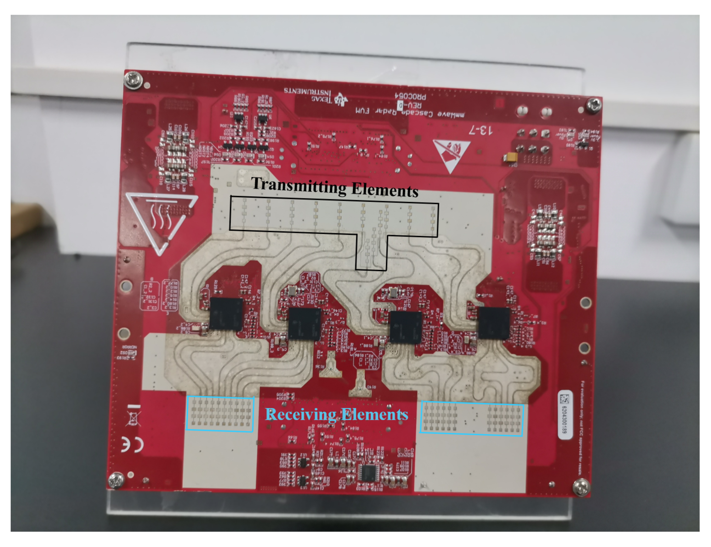
We performed follow-up work on Texas Instruments’ cascaded FMCW-MIMO radar systems (MMWAVCAS-RF-EVM and MMWAVCAS-DSP-EVM). As shown in Figure 1, this FMCW-MIMO radar has 16 receiving and 12 transmitting elements. With these array elements, the radar can form a large virtual array. However, in this paper, only a small fraction of the uniform linear array (ULA) of this FMCW-MIMO radar virtual array element (the first 10 arrays, as shown in Figure 2) are taken to achieve the case we envision.
From [7], the signal of the FMCW-MIMO radar transmitting by the transmitting array element to the receiving array element can be expressed as:
where is the carrier frequency, and is the slope of the chirp. Assume that there are K far-field narrow-band targets. Then, the signal received at the i-th receiving element can be expressed as:
where is the additive Gaussian white noise of the i-th receiving element, is the complex reflection coefficient of the j-th target, and is the time delay required for the signal emitted from the transmitting elements to reach the i-th receiving element through the j-th target reflection. There is a direct relationship between and the distance between the target and the FMCW-MIMO radar. The detail relationship is:
where c, and are the speed of light, the amount of distance between the j-th target and the transmitting element and amount of distance between the j-th target and the i-th receiving element; is the distance between the i-th receiving element and the first receiving element (reference starting point); and is the DOA of the j-th target.
The received signal is obtained by multiplying the transmitted signal and the reflected signal, and then passing it through a low-pass filter with sampling time . After conversion into a digital signal, x can be expressed as follows:
It can be summarized that for an FMCW system with M receiver and N snapshots, the signals from receiving K targets can be expressed as follows:
where is complex Gaussian noise with covariance ; , ; and , .
3. Proposed Multi-DeepNet Architecture
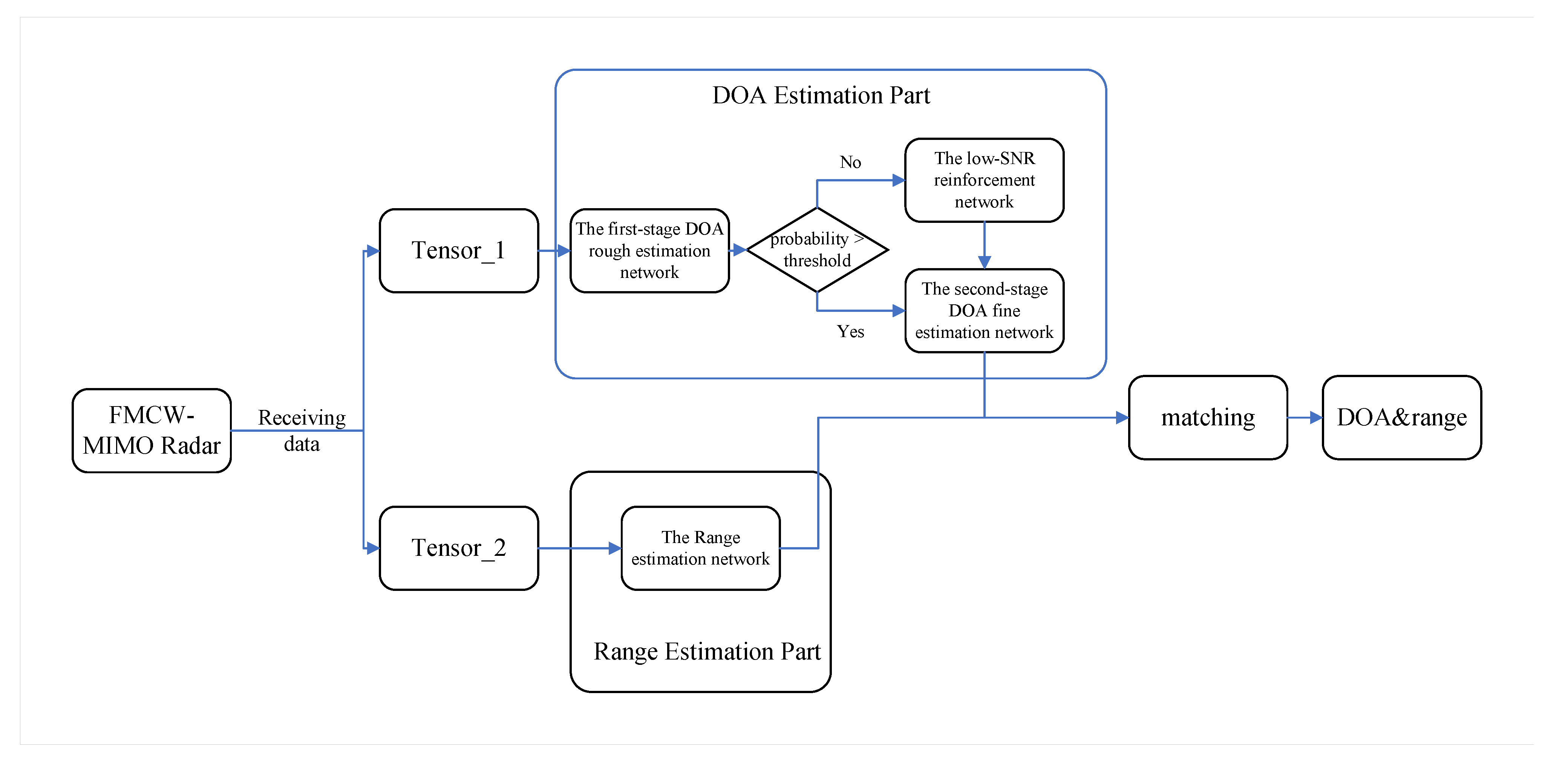
The DL framework for estimating DOA, the DL framework for estimating range and the matching methods are presented separately in this section. The complete estimation process is shown in Figure 3.
The specific workflow of the proposed Multi-DeepNet is as follows. First, we obtain the sampling covariance matrix from the received data .
Then, a three-channel tensor is formed by taking out the real part, imaginary part and phase of , i.e.,
This tensor is then fed into the first-stage rough DOA estimation network. The first-stage rough DOA estimation network allows us to obtain the range ( as an interval) of the angle grid. To enhance the performance at low SNRs, the network checks the results of the first-stage rough DOA estimation network. If the results do not satisfy the requirements, the low-SNR reinforcement network intervenes. Otherwise, the corresponding second-stage fine DOA estimation network is selected to be called based on the result of the first-order rough DOA estimation network. With the second-stage fine DOA estimation network, we can then obtain DOA estimates with a grid of .
After obtaining the estimates of DOA, we obtain the transposed received signal covariance matrix as:
Again, we stitch the real part, imaginary part and phase of to form a tensor . The tensor is fed into the range estimation network, and with this distance estimation network we can directly obtain the range estimate with a grid of .
Finally, we match the obtained DOA and range estimates to achieve joint angle and range estimation.
3.1. Introduction to the Multi-DeepNet Layers
According to [23], the 2D convolutional layer in the Multi-DeepNet can be described as follows:
where is the output of the 2D convolutional layer, is the batch-size, and is the number of out channels. is the weight of the kernel, and is the bias of the 2D convolutional layer.
From [24], a dense layer, widely used in a variety of DNNs, can be derived as follows:
where , , and are the output, weight, input and bias of the dense layer in the Multi-DeepNet.
In order to preserve the effect of negative numbers during 2D convolution, leakyReLU is used as the activation function behind the 2D convolution layer in the framework. According to [25,26], ReLU and leakyReLU can be described as:
where is preset leaky value, typically set to .
Additionally, it is available from [27]. The batch normalization layer can be represented as follows:
where and are learnable parameters. Depending on the output of the previous layer above the batch normalization layer, the x can be either a vector or a matrix.
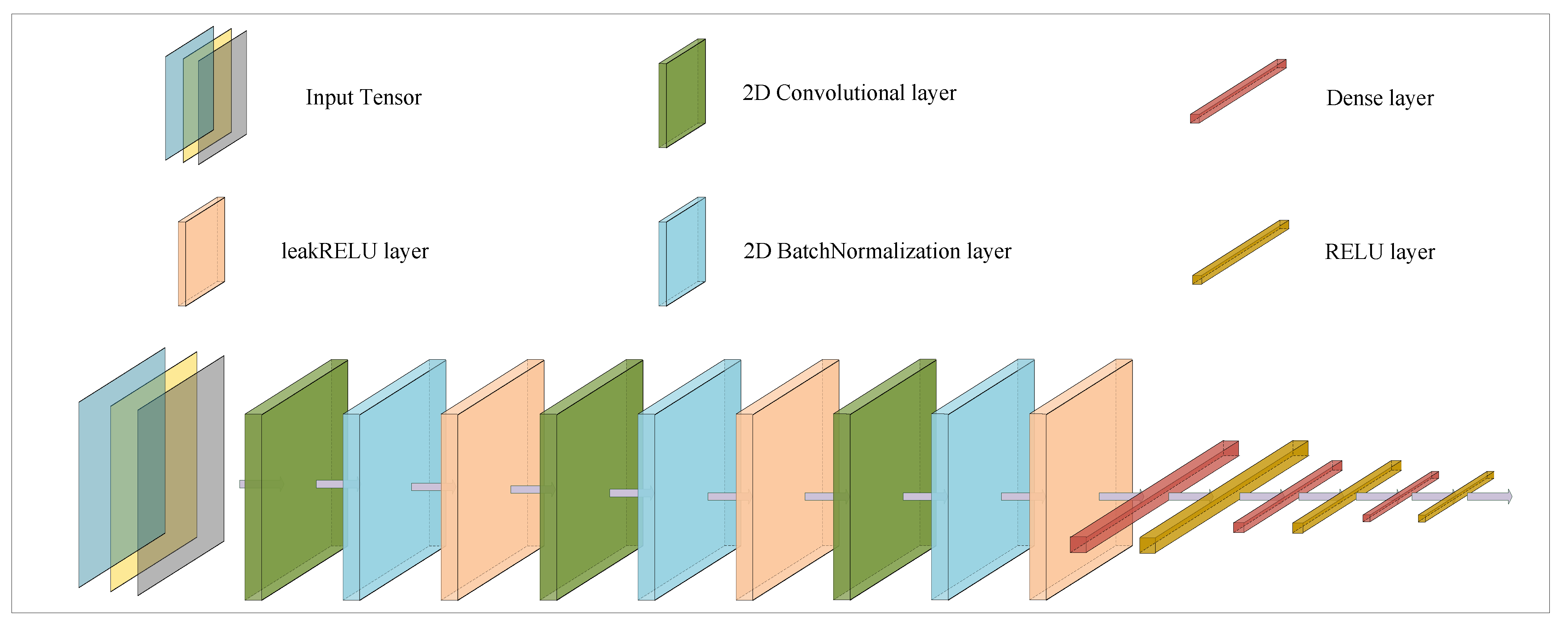
3.2. The First-Stage DOA Rough Estimation Network Structure
In this part, as part of the DOA estimations for the interval to , 12 small intervals of each are considered, the first-stage rough DOA estimation network structure is shown in Figure 4.
The input layer receives the assembled by the received data sampling covariance matrix, as in Equations (6) and (7), to extract the high-dimensional features of the sampled covariance matrix. This will be passed through a 2D convolutional layer to accelerate the learning speed and strengthen the NN’s ability to learn from the data. The above data is fed into the 2D batch normalization layer of the same scale after passing through the 2D convolutional layer. For the choice of activation function, we choose to use leaky RELU in order to avoid the disadvantage that the RELU function is too fragile on deep networks.
After passing through the three 2D convolutional layers, batch normalization layers and activation function layers, the data are unfolded by the flatten operation and fed into the dense layer. Then, after passing through the three dense layers, the probability of DOA occurrence in each interval is obtained. The detailed structural parameters of the first-stage rough DOA estimation network are shown in Table 1.
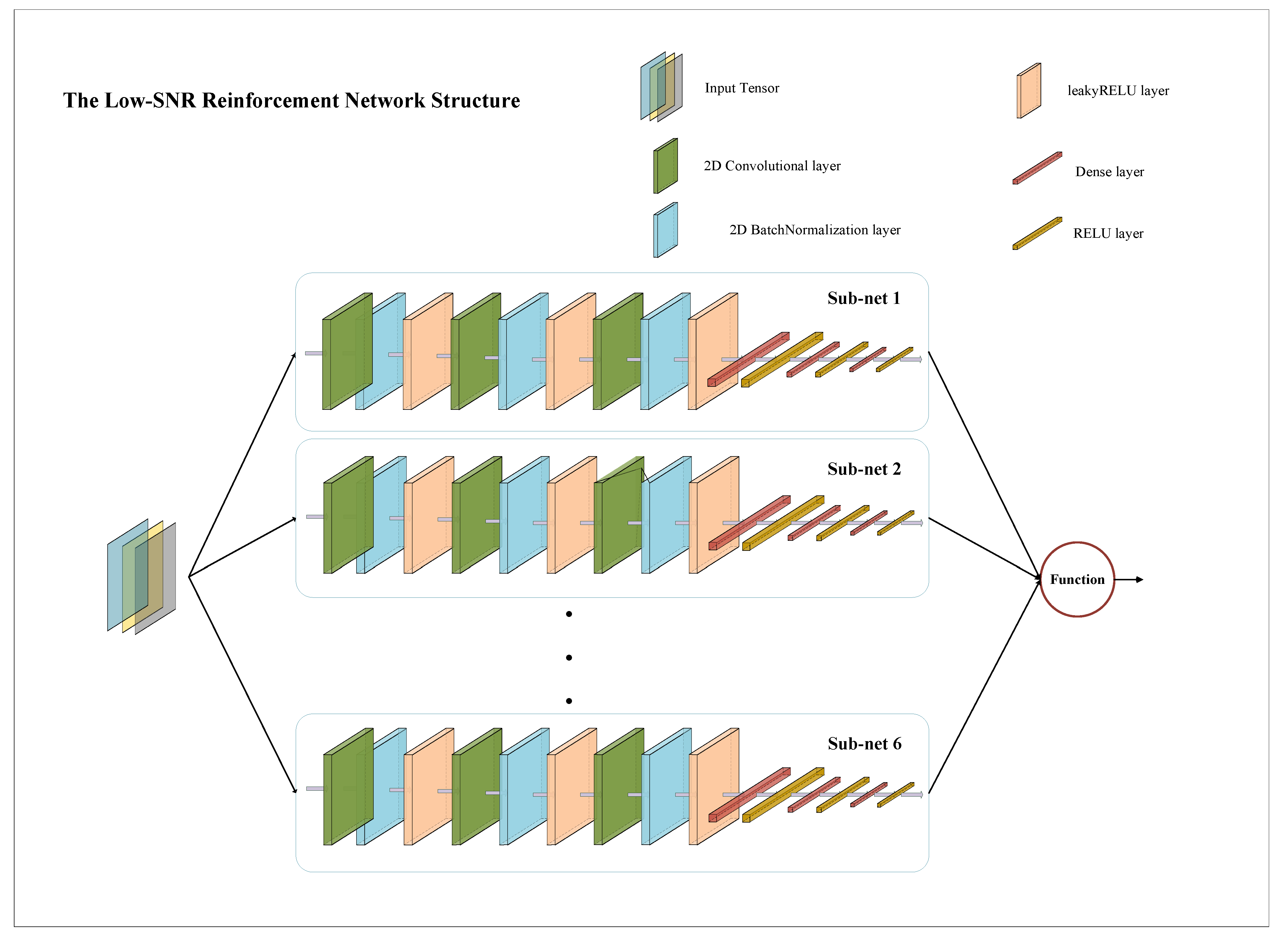
3.3. The Low-SNR Reinforcement Network Structure
The first-stage network is not always able to estimate the angle interval accurately when the SNR is low. It is for this reason that low-SNR reinforcement networks (LSR-net) are proposed. When the probability (maximum value) estimated by the network is less than the threshold set initially, the LSR-net is invoked. Otherwise, the second-stage DOA estimation is performed directly.
The whole LSR-net is composed of six subnetworks, each of which has the same structure as that of the first-stage network, as shown in Figure 5. Finally, a combinatorial function is used to find the final probability distribution, which is denoted by
where is the output of LSR-net, and is the output of k-th subnetwork. On the basis of , we determine which second-stage networks should be invoked.
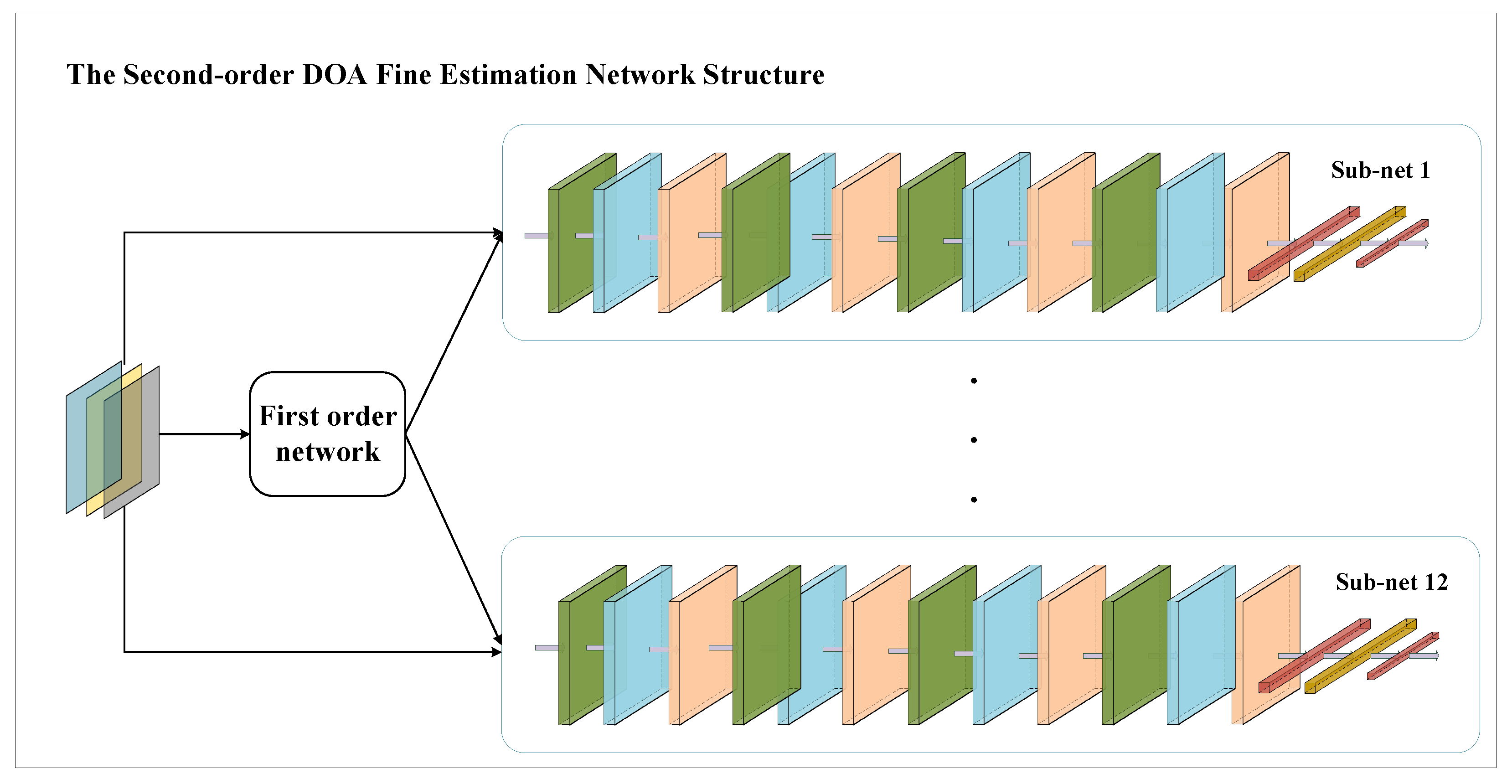
3.4. The Second-Order DOA Fine Estimation Network Structure
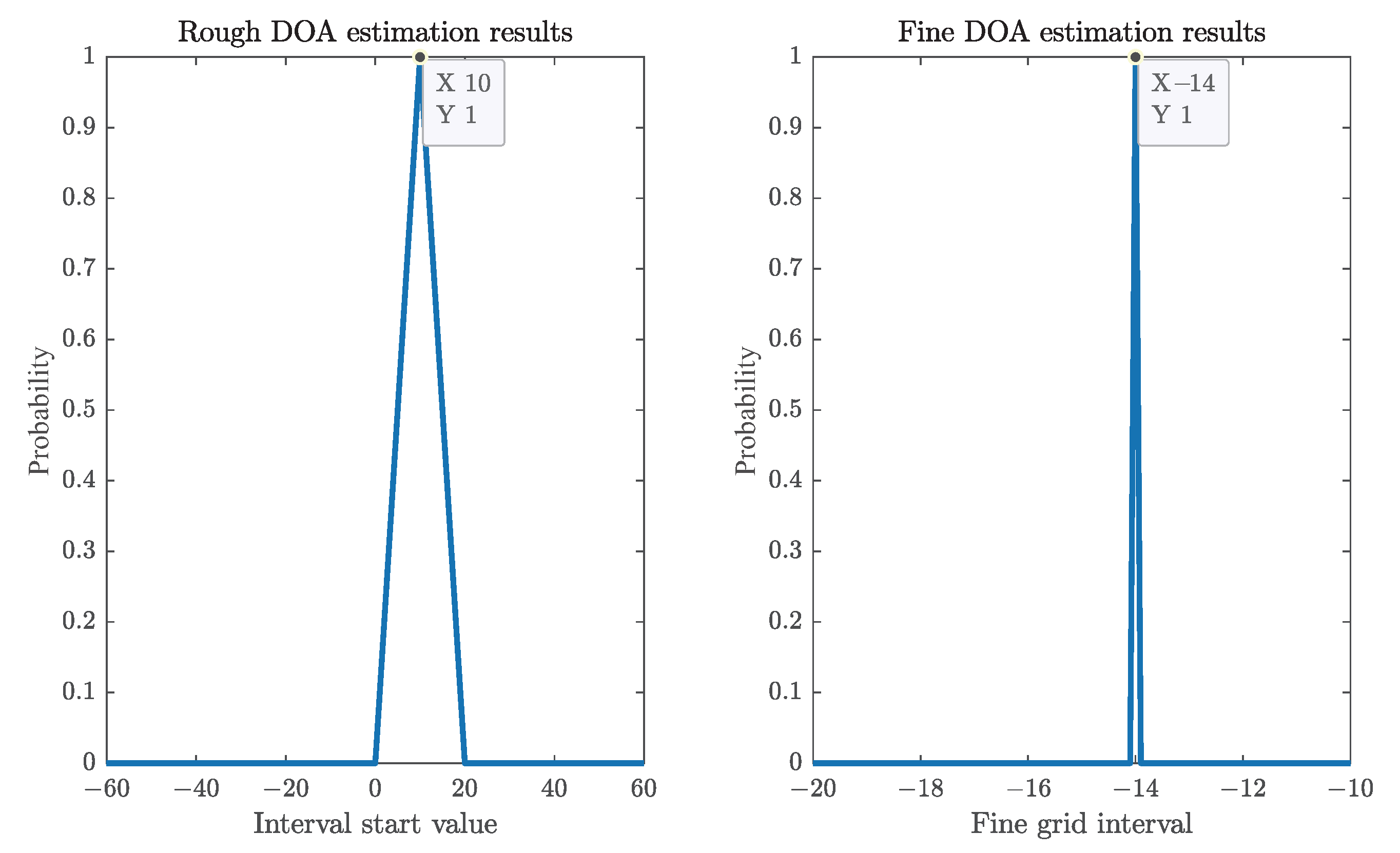
With the network of the two subsections mentioned above, we obtain the interval in which the angle is located. After obtaining the interval where the angle is located, the second-stage DOA fine estimation network is invoked for the corresponding interval. Thus, 12 structurally consistent subnetworks were designed, and the coarse estimation results were used to choose the subnetworks that call the intervals. The tensor is fed into the subnetwork as shown in Figure 6, and the final result is the peak value of the spectral peak in the corresponding interval, as shown in Figure 7. (The simulation in the figure is based on the m, dB.)
We optimized the corresponding structure for dense data based on the first-stage of the network. The parameters of the second-order DOA fine estimation network are specified in Table 2. The in Table 2 define leakyReLU and BN as shown in the tab leakyReLU.1 and BN.1.
The estimation of DOA is completed when the results of the second-order DOA fine estimation network are obtained.
3.5. The Range Estimation Network Structure
For the range estimation, Equation (8) provides the covariance of the received data transposition from the FMCW-MIMO radar. From Equation (9), we can obtain as the input for the range estimation network.
The interval of our considered range is from 1 m to 10 m, and the size of the grid is 0.1 m. The amount of data involved in range estimation is much smaller than that in the DOA estimation part. Therefore, in the range estimation part, we only design one deep neural network to implement fine range estimation.
Our proposed range estimation network is structurally similar to the first-stage rough DOA estimation network described above. Both are based on the aggregation of CNN and dense networks. The parameters of the detailed range estimation network are shown in Table 3.
With the range estimation network described above, a pseudo-spectrum of the range is obtained, and the spectral peak is the value where the maximum probability of the range occurrence is located.
3.6. Matching Method
If there are multiple targets (multiple pairs of DOA and range), we need to consider the matching problem. From Equations (4) and (5), we know that DOA and range are coupled in the received signal. So in case of mismatch, the received signal will be dramatically different from the we constructed using the known DOA and range. However, in the case of correct pairing, the difference will be small.
Based on the above, we transform the matching problem into a problem of finding the minimum value. The pseudo-code is shown in Algorithm 1:
| Algorithm 1 Matching Method. |
|
4. Simulations and Experiments
In order to validate the proposed method, several simulations and experiments are conducted. According to Table 4, simulations and experiments have the same TI Cascade FMCW-MIMO radar parameters.
4.1. Cramer–Rao Bounds for FMCW MIMO-Radar
Cramer–Rao bounds, also known as the Cramer–Rao lower bounds (CRLB), are proposed for parameter estimation problems and establish lower bounds for the variance of any unbiased estimator. The variance of the unbiased estimator can only approach the CRB without restriction and will not fall below the CRB.
Then, the covariance matrix . is given by
where and , . Therefore, by setting , we can obtain:
The CRB of and can be obtained according to the Cramer criterion as
In the following subsections, we first describe the data generation, training environment and methods. Then, we compare several classical methods in the simulation of estimating DOA. After that, we compare several classical methods in the simulation of estimating range. Based on this, we compare the localization error of the algorithm. Next, we test the running speed of the algorithm. Finally, we apply the algorithm to experimental data.
4.2. Data Generation, Training Environment and Methods
The platform for the experiment is a PC with an Intel i7-12700H CPU 2.2 GHz, RTX 3070 laptop GPU and 16 GB of RAM. The experimental environment is Matlab 2022a and tensorflow 2.90. For the Multi-DeepNet optimizer we chose to use Adam with default parameters. The maximum value of epochs was set to 100, and the size of batch-size was set to 64. In the proposed Multi-DeepNet, training time was not taken into account since the training procedure was off-line.
To generate the training data of Multi-DeepNet, we assumed that the DOA of n sources was located at to and range was located at 1 m to 10 m. First, we randomly selected the number of incident signal sources n between one tosix, then we randomly selected n DOAs between intervals to , and n ranges between intervals 1 m to 10 m. Using the pair of DOAs and ranges generated above, we generated the corresponding radar received signal through Equations (4) and (5), and converted the received signal into the tensor received by the network through Equations (6)–(9). For the pair of DOA and range generated above, we first labeled the sector where the DOA was located, and then we labeled the pseudo-spectrum where the range was located. In this way, we can obtain a set of training data of the first-stage rough DOA estimation network and range estimation network . For the above pair of DOA and range, we will generate training data under different SNRs −20 dB to 20 dB. At each SNR, we generated 500,000 sets of data.
Low-SNR reinforcement network training data are similar to the first-stage rough DOA estimation data. The difference is only in SNRs of training data. The data of low-SNR reinforcement network only considers −20 dB to 0 dB.
The training data for each sub-net of the second-order DOA fine estimation network were generated separately. For example, in sub-net 1, the DOA of our training data was only randomly generated between and , and the generation method of range remained unchanged. Finally, 500, 000 sets of data were generated for each SNR between −20 dB and 20 dB.
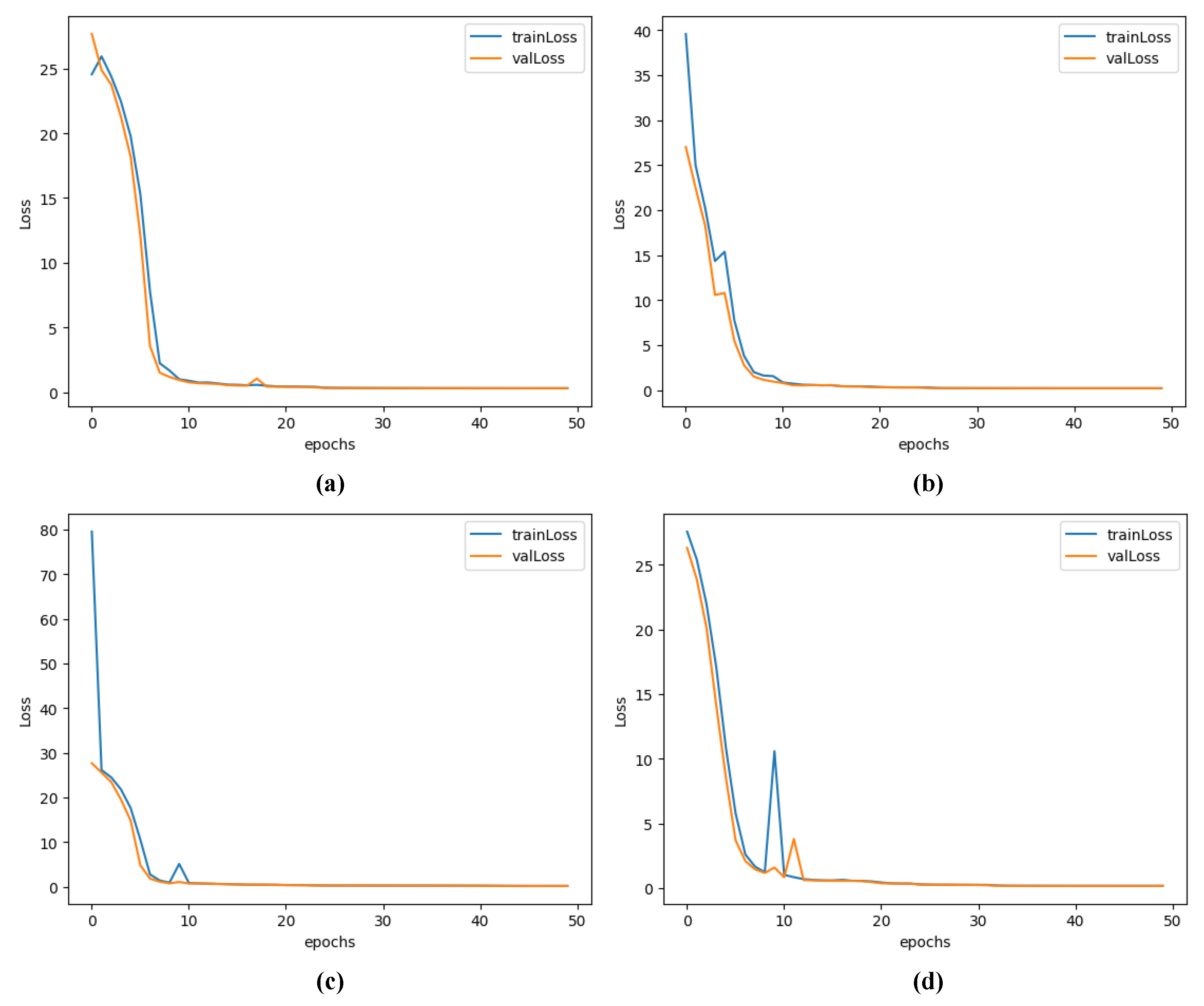
When training the Multi-DeepNet, the corresponding training data was randomly divided into training set and validation set. The training history of the Multi-DeepNet is shown in Figure 8. In the figure, (a), (b), (c) and (d), respectively, describe the training history of the first-stage rough DOA estimation network, the low-SNR reinforcement network, the second-order DOA fine estimation network and the range estimation network. It can be seen from e Figure 8 that validation losses and training losses were always close during training, and they coincided at the end, indicating no overfitting.
4.3. Simulations
Two far-field narrow-band fixed targets at , 2.5 m) and , 7.5 m) were considered to verify the performance of the whole Multi-DeepNet. DOA and range were evaluated using the root mean square error (RMSE) metric. We define the RMSE equations for DOA, range and location separately as follows:
where and are the k-th true DOA and range, and are the k-th estimated values of DOA and range in the m-th Monte Carlo trial, is the k-th target actual location, and is the k-th estimated values of location in the m-th Monte Carlo trial. We represent DOA and range in a right-angle coordinate system as shown in the following equation:
We set the number of Monte Carlo experiments M to 200. In addition, we performed a runtime comparison of various algorithms as a way to demonstrate the advantages of real-time performance of the Multi-DeepNet.
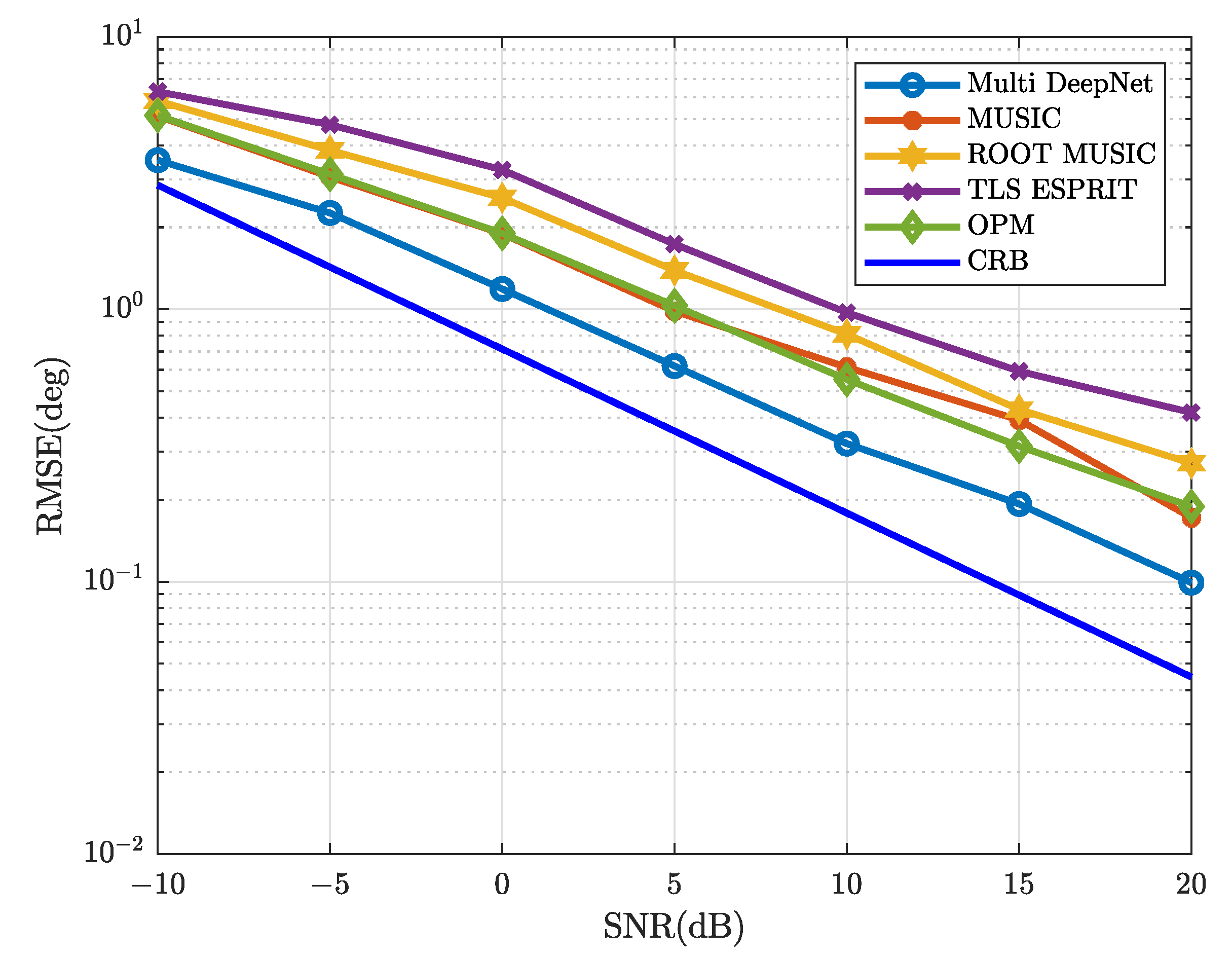
We adopted several traditional DOA estimation methods to compare with the proposed Multi-DeepNet in the simulation setup of DOA estimation. Examples are MUSIC with Grid [5,6], the OPM algorithm [29], the TLS-ESPRIT algorithm [10] and the ROOT-MUSIC algorithm [30]. As shown in Figure 9, we set and = [2.72 m, 8.72 m], deliberately placing the DOA outside the grid, with some grid error. When the SNR increases, the Multi-DeepNet has better performance than other algorithms.
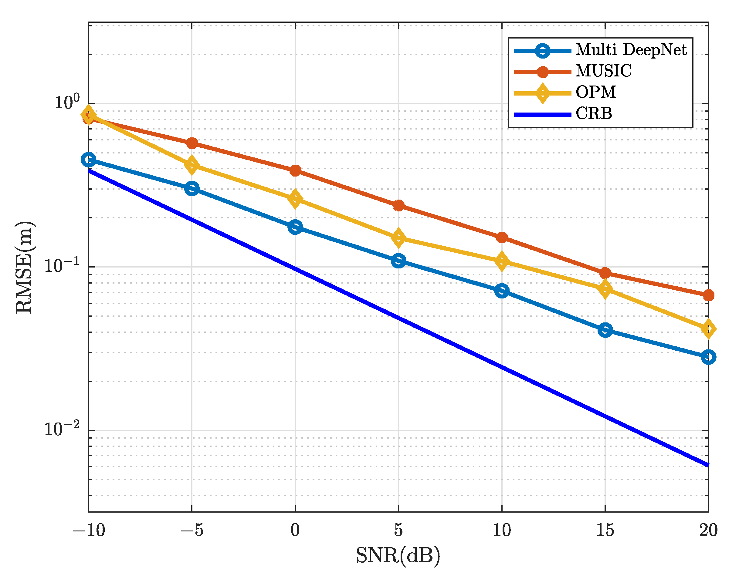
In the simulation of range estimation, we chose the same DOA and range of the above simulation to generate the simulation data. Since range estimation involves fewer algorithms, we only compared the performance differences among MUSIC with Grid , OPM and Multi-DeepNet. As shown in Figure 10, it can be seen that the RMSE curve of Multi-DeepNet at −10 dB to 20 dB SNR was always located below the RMSE curve of the other two algorithms.
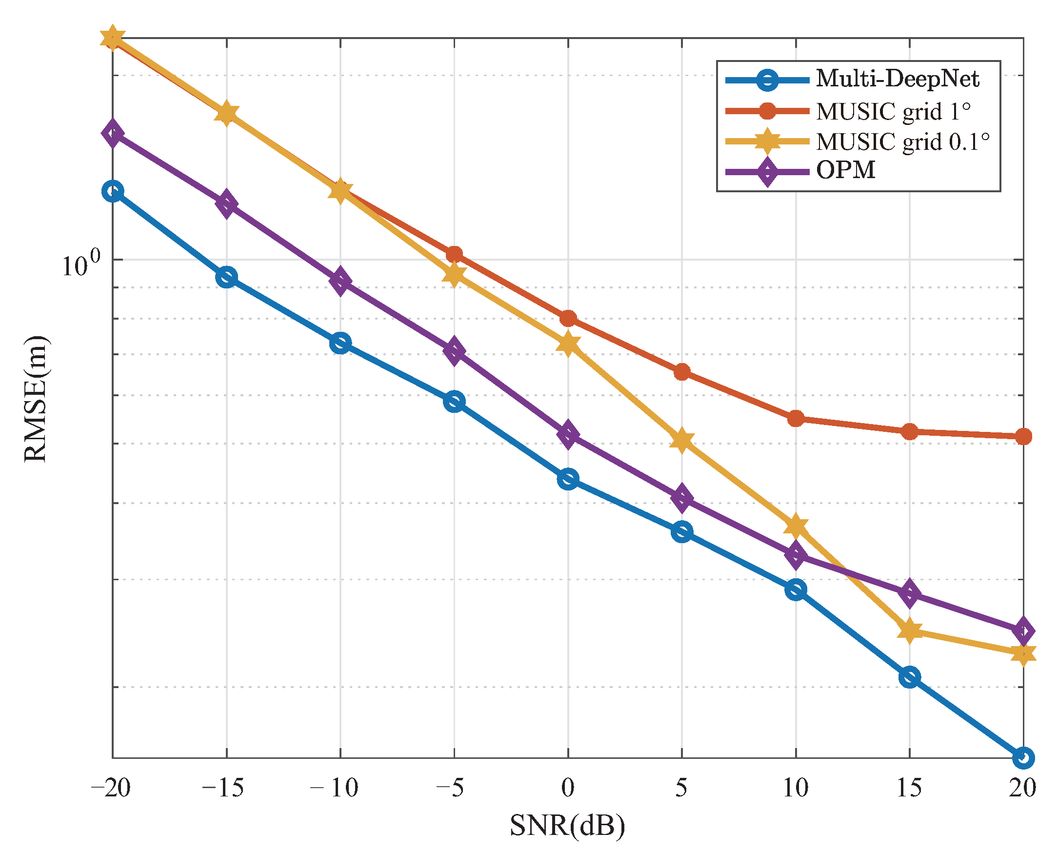
In the joint estimation, we generally converted DOA and range into a right-angle coordinate system for the comparison of RMSE as in Equation (28). We used MUSIC with Grid , MUSIC with Grid , OPM, and Multi-DeepNet for the comparison as shown in Figure 11. The simulation showed that Multi-DeepNet has a clear advantage in the SNR range of −20 dB to 20 dB. Multi DeepNet can achieve better performance than other algorithms under low SNR ratio due to the combination of reinforcement training under low SNR and multiple low-SNR reinforcement networks.
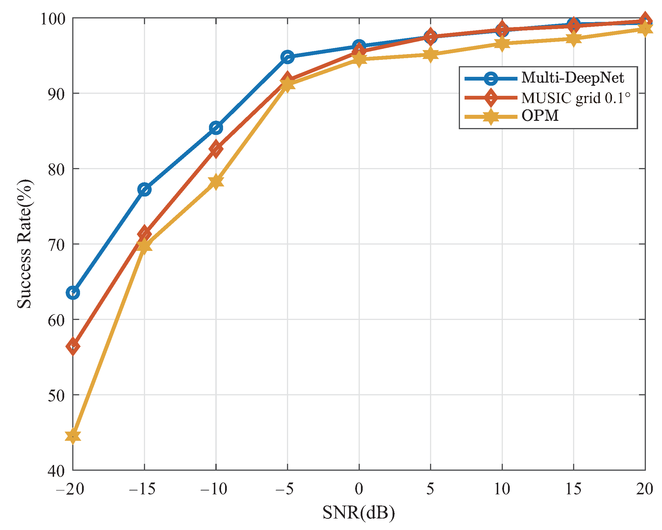
Other than the above simulations, the success rate of the algorithm localization was tested in this paper. The success rate can be defined as the ratio of the number of Monte Carlo simulations to the number of times the difference between the localized result and the true value is less than a threshold. In this simulation, the threshold was set to and the number of Monte Carlo simulations was 200. In the simulation result, Figure 12, the success rate of the algorithm was acceptable at a low signal-to-noise ratio. The success rate at high signal-to-noise ratio also had a good level.
In addition, the simulation in Figure 13 shows the running time comparison, and we can clearly see that Multi-DeepNet has a much lower time requirement than other algorithms. Because the modules formed by Multi DeepNet are all simple matrix operations, they are faster than other algorithms.
4.4. Experiments
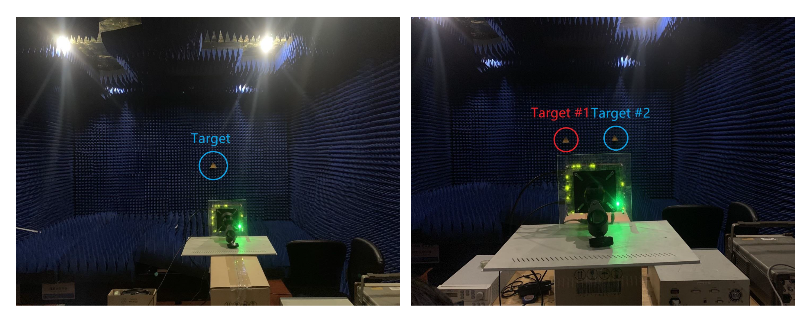
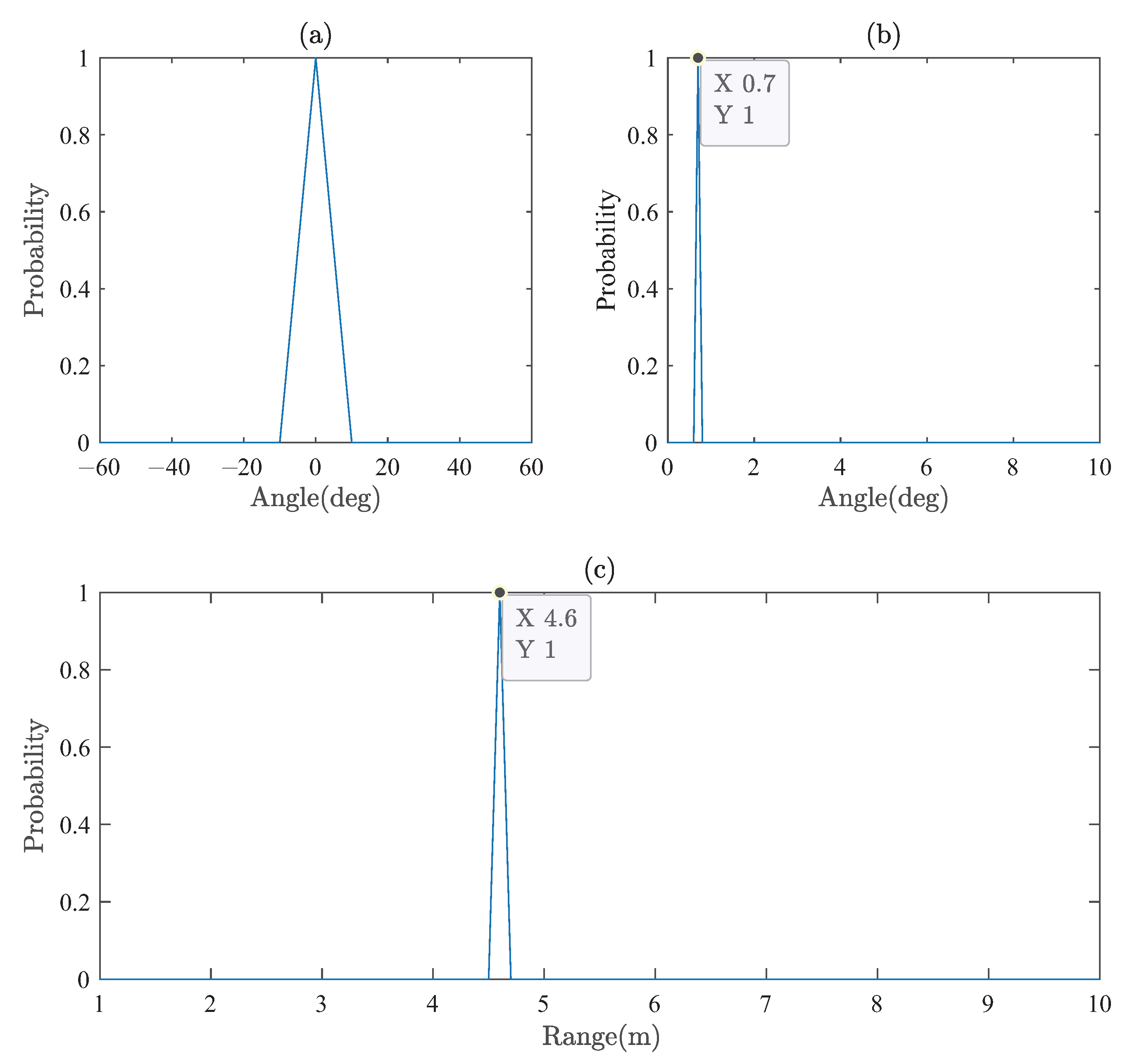
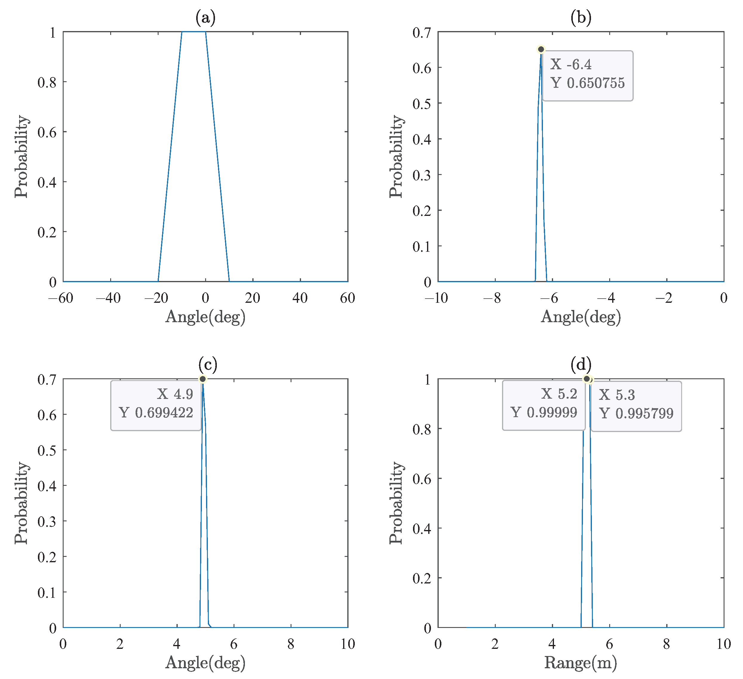
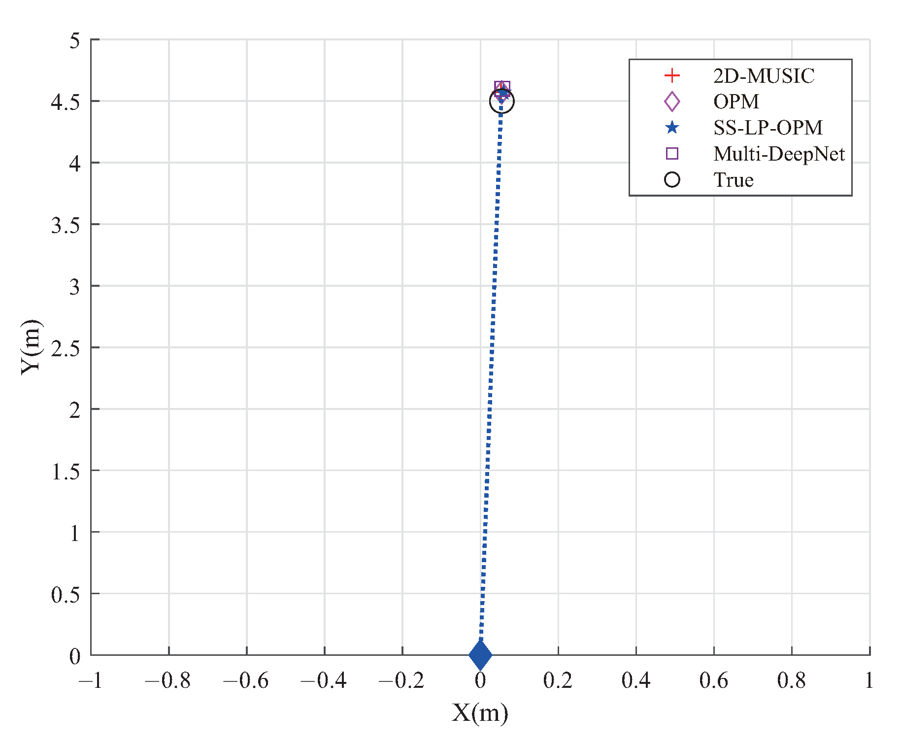
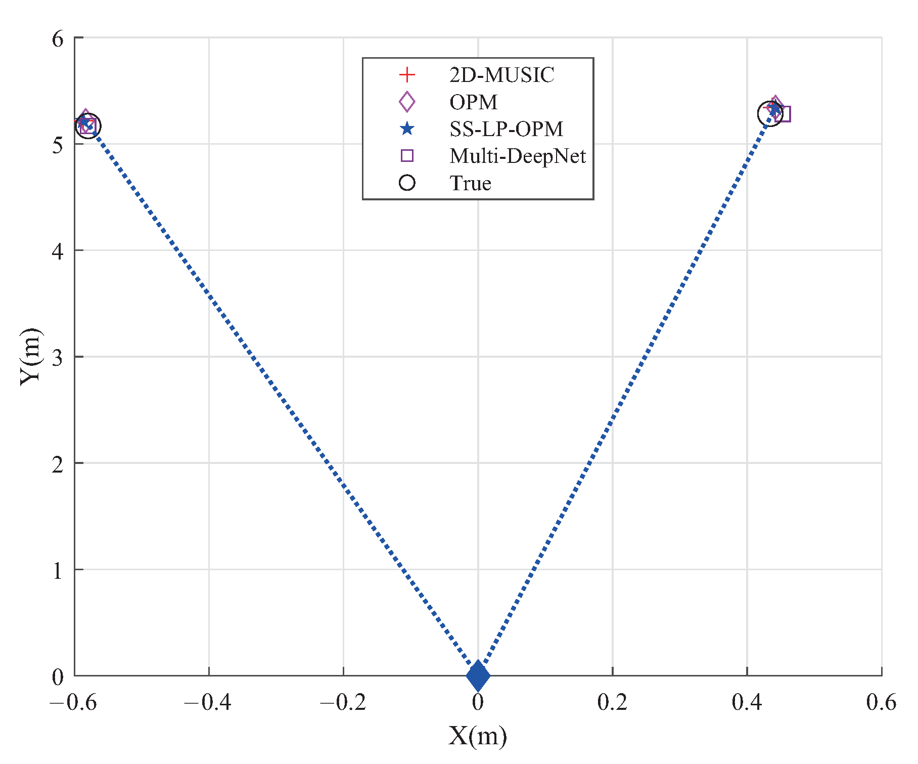
To fix the poor calibration in [22], a calibration matrix certified in a darkroom environment was used. The experimental data were obtained from the TI Cascade FMCW-MIMO Radar shown in Figure 1. The location of the experiment was a microwave darkroom, and the detection target of the experiment was the metal corner reflector. We measured two different scenarios throughout the experiment. The two scenarios are shown in Figure 14: target set at , 4.5 m) in Scenario 1 and target set at , 5.2 m) and , 5.3 m) in Scenario 2. The locationing effect was selected as a performance metric in this part of the study. In the experiment, the SNR of Scenario 1 was 20 dB, and that of Scenario 2 was 15 dB.
The estimated results of the Multi-DeepNet on the measured data are sh. When the SNR increases, the Multi-DeepNet still has better performance than other algorithms shown in Figure 15 and Figure 16, respectively. Figure 15 is the single target scenario: (a) is the estimated result of the first-stage rough DOA estimation network, (b) is final DOA estimation result, and (c) is the estimated range. The predicted DOA and range can be obtained directly by observing the output value of the Multi-DeepNet.
Figure 16 shows the results of the two target scenarios: (a) is the rough DOA estimation result, (b) and (c) are final DOA estimation results, and (d) is the estimated range. In the following section, we compare the results of Multi-DeepNet with that of other algorithms.
Figure 17 and Figure 18 show the comparison of the localization results of the proposed algorithm with 2D-MUSIC, OPM and SS-LP-OPM on experimental data. It can be seen that several algorithms have good performance on the experimental data, and there is no significant difference with the real position. As can be seen from the two experimental graphs, the proposed localization framework is practically feasible.
5. Conclusions
In this paper, we have proposed a fast joint DOA and range estimation framework based on deep learning for target localization. With the proposed algorithm, better estimation performance with low signal-to-noise ratio and fewer snapshots can be achieved while reducing the required running time. The simulations show that the proposed algorithm has significant advantages in the case of low SNR and low snapshot, and satisfactory performance in the case of higher SNR. Finally, experimental data are also supplemented for verification. Although the proposed algorithm has good results, there are still some problems such as not having significant advantages at high SNR and the overall framework being too complex. Therefore, in subsequent work, the structure of the framework and network can be simplified to improve the performance under high SNR.
Author Contributions
Conceptualization, X.W. and L.S.; methodology, Y.S. and X.W.; writing—original draft preparation, Y.S.; writing—review and editing, X.W. and J.S.; supervision, X.W. and X.L.; funding acquisition, X.W. and X.L. All authors have read and agreed to the published version of the manuscript.
Funding
This work was supported by Natural Science Foundation of Hainan Province (620RC555), the National Natural Science Foundation of China (No. 61861015, 61961013, 62101088), Radar Signal Processing National Defense Science and Technology Key Laboratory Fund (6142401200101).
Data Availability Statement
Not applicable.
Conflicts of Interest
The authors declare no conflict of interest.
Nomenclature
The following nomenclature are used in this manuscript:
| conjugate-transpose operator | |
| transpose operator | |
| the Frobenius norm operator | |
| the 2-norm operator | |
| the real part operator | |
| the imag part operator | |
| the Phases part operator | |
| the expectation operator | |
| the variance operator | |
| identity matrix | |
| 🟉 | 2D cross-correlation operator |
| dimensional complex matrix set | |
| dimensional rational numbers matrix set |
References
- Brennan, P.V.; Huang, Y.; Ash, M.; Chetty, K. Determination of Sweep Linearity Requirements in FMCW Radar Systems Based on Simple Voltage-Controlled Oscillator Sources. IEEE Trans. Aerosp. Electron. Syst. 2011, 47, 1594–1604. [Google Scholar] [CrossRef]
- Waldschmidt, C.; Hasch, J.; Menzel, W. Automotive Radar—From First Efforts to Future Systems. IEEE J. Microwaves 2021, 1, 135–148. [Google Scholar] [CrossRef]
- Stove, A.G. Linear FMCW radar techniques. IEE Proc. F Radar Signal Process. 1992, 139, 343–350. [Google Scholar] [CrossRef]
- Alizadeh, M.; Shaker, G.; De Almeida, J.C.M.; Morita, P.P.; Safavi-Naeini, S. Remote Monitoring of Human Vital Signs Using mm-Wave FMCW Radar. IEEE Access 2019, 7, 54958–54968. [Google Scholar] [CrossRef]
- Wang, X.; Wan, L.; Huang, M.; Shen, C.; Han, Z.; Zhu, T. Low-complexity channel estimation for circular and noncircular signals in virtual MIMO vehicle communication systems. IEEE Trans. Veh. Technol. 2021, 69, 3916–3928. [Google Scholar] [CrossRef]
- Wang, X.; Huang, M.; Wan, L. Joint 2D-DOD and 2D-DOA Estimation for Coprime EMVS–MIMO Radar. Circuits Syst. Signal Process. 2021, 40, 2950–2966. [Google Scholar] [CrossRef]
- Feger, R.; Wagner, C.; Schuster, S.; Scheiblhofer, S.; Jager, H.; Stelzer, A. A 77-GHz FMCW-MIMO Radar Based on an SiGe Single-Chip Transceiver. IEEE Trans. Microw. Theory Tech. 2009, 57, 1020–1035. [Google Scholar] [CrossRef]
- Belfiori, F.; van Rossum, W.; Hoogeboom, P. 2D-MUSIC technique applied to a coherent FMCW-MIMO radar. In Proceedings of the IET International Conference on Radar Systems (Radar 2012), Glasgow, UK, 22–25 October 2012; pp. 1–6. [Google Scholar]
- Lee, J.; Hwang, S.; You, S.; Byun, W.J.; Park, J. Joint angle, velocity, and range estimation using 2D MUSIC and successive interference cancellation in FMCW-MIMO radar system. IEICE Trans. Commun. 2020, 103, 283–290. [Google Scholar] [CrossRef]
- Cong, J.; Lu, T.; Bin, Z.; Jing, X.; Wang, X. A Gridless Joint DOA and Range Estimation Method for FMCW-MIMO Radar. Smart Commun. Intell. Algorithms Interact. Methods 2022, 257, 315–321. [Google Scholar]
- Hamidi, S.; Naeini, S.S. TDM based Virtual FMCW-MIMO Radar Imaging at 79 GHz. In Proceedings of the 2018 18th International Symposium on Antenna Technology and Applied Electromagnetics (ANTEM), Waterloo, ON, Canada, 19–22 August 2018; pp. 1–2. [Google Scholar]
- Cong, J.; Wang, X.; Huang, M.; Bi, G. Feasible Sparse Spectrum Fitting of DOA and Range Estimation for Collocated FDA-MIMO radars. In Proceedings of the 2020 IEEE 11th Sensor Array and Multichannel Signal Processing Workshop (SAM), Hangzhou, China, 8–11 June 2020; pp. 1–5. [Google Scholar]
- Cong, J.; Wang, X.; Lan, X.; Wan, L. Fast Target Localization Method for FMCW-MIMO Radar. In Proceedings of the 2021 IEEE MTT-S International Wireless Symposium (IWS), Nanjing, China, 23–26 May 2021; pp. 1–3. [Google Scholar]
- Wang, W.; Wang, X.; Shi, J.; Lan, X. Joint Angle and Range Estimation in Monostatic FDA-MIMO Radar via Compressed Unitary PARAFAC. Remote Sens. 2022, 14, 1398. [Google Scholar] [CrossRef]
- Wang, W.; Lan, X.; Shi, J.; Wang, X. A Fast PARAFAC Algorithm for Parameter Estimation in Monostatic FDA-MIMO Radar. Remote Sens. 2022, 14, 3093. [Google Scholar] [CrossRef]
- Ahmed, A.M.; Thanthrige, U.S.K.M.; El Gamal, A.; Sezgin, A. Deep Learning for DOA Estimation in MIMO Radar Systems via Emulation of Large Antenna Arrays. IEEE Commun. Lett. 2021, 25, 1559–1563. [Google Scholar] [CrossRef]
- Barthelme, A.; Utschick, W. DoA Estimation Using Neural Network-Based Covariance Matrix Reconstruction. IEEE Signal Process. Lett. 2021, 28, 783–787. [Google Scholar] [CrossRef]
- Papageorgiou, G.K.; Sellathurai, M.; Eldar, Y.C. Deep Networks for Direction-of-Arrival Estimation in Low SNR. IEEE Trans. Signal Process. 2021, 69, 3714–3729. [Google Scholar] [CrossRef]
- Cong, J.; Wang, X.; Huang, M.; Wan, L. Robust DOA Estimation Method for MIMO Radar via Deep Neural Networks. IEEE Sens. J. 2020, 21, 7498–7507. [Google Scholar] [CrossRef]
- Cong, J.; Wang, X.; Wan, L.; Huang, M. Neural Network-Aided Sparse Convex Optimization Algorithm for Fast DOA Estimation. Trans. Inst. Meas. Control 2022, 44, 1649–1655. [Google Scholar] [CrossRef]
- Cong, J.; Wang, X.; Yan, C.; Yang, L.T.; Dong, M.; Ota, K. CRB Weighted Source Localization Method Networks in Multi-UAV Network. IEEE Internet Things J. 2022. [Google Scholar] [CrossRef]
- Cong, J.; Wang, X.; Lan, X.; Huang, M.; Wan, L. Fast Target Localization Method for FMCW-MIMO Radar via VDSR Neural Network. Remote Sens. 2021, 13, 1956. [Google Scholar] [CrossRef]
- LeCun, Y.; Bottou, L.; Bengio, Y.; Haffner, P. Gradient-based learning applied to document recognition. Proc. IEEE 1998, 86, 2278–2324. [Google Scholar] [CrossRef] [Green Version]
- Pal, S.K.; Mitra, S. Multilayer perceptron, fuzzy sets, and classification. IEEE Trans. Neural Netw. 1992, 3, 683–697. [Google Scholar] [CrossRef]
- Glorot, X.; Bordes, A.; Bengio, Y. Deep sparse rectifier neural networks. In Proceedings of the Fourteenth International Conference on Artificial Intelligence and Statistics. JMLR Workshop and Conference Proceedings, Fort Lauderdale, FL, USA, 11–13 April 2011; Volume 15, pp. 315–323. [Google Scholar]
- Maas, A.L.; Hannun, A.Y.; Ng, A.Y. Rectifier nonlinearities improve neural network acoustic models. In Proceedings of the 30th International Conference on International Conference on Machine Learning (ICML’13), Atlanta, GA, USA, 16–21 June 2013; Volume 30, p. 3. [Google Scholar]
- Ioffe, S.; Szegedy, C. Batch normalization: Accelerating deep network training by reducing internal covariate shift. In Proceedings of the International Conference on Machine Learning (PMLR), Lille, France, 6–11 July 2015; pp. 448–456. [Google Scholar]
- Kim, J.; Chun, J.; Song, S. Joint range and angle estimation for FMCW-MIMO radar and its application. arXiv 2018, arXiv:1811.06715. [Google Scholar]
- Marcos, S.; Marsal, A.; Benidir, M. The propagator method for source bearing estimation. Signal Process. 1995, 42, 121–138. [Google Scholar] [CrossRef]
- Rao, B.D.; Hari, K.S. Performance analysis of Root-Music. IEEE Trans. Acoust. Speech Signal Process. 1989, 37, 1939–1949. [Google Scholar] [CrossRef]
Figure 1.
Texas Instruments’ cascaded FMCW-MIMO radar systems.

Figure 2.
The selected elements and the remaining receiving elements.

Figure 3.
The complete estimation process of Multi-DeepNet.

Figure 4.
Structure of the first-stage rough DOA estimation network.

Figure 5.
The low-SNR reinforcement network structure.

Figure 6.
The second-order DOA fine estimation network structure.

Figure 7.
DOA estimation example.

Figure 8.
Training history of Multi-DeepNet.

Figure 9.
RMSE of DOA estimation with SNR.

Figure 10.
RMSE of range estimation with SNR.

Figure 11.
RMSE of location estimation with SNR.

Figure 12.
Success rate with SNR.

Figure 13.
The average running time varies with the number of run trials.

Figure 14.
The experiments in Scenario 1 and Scenario 2.

Figure 15.
DOA and range estimation result of Scenario 1.

Figure 16.
DOA and range estimation of Scenario 2.

Figure 17.
Localization result of Scenario 1.

Figure 18.
Localization result of Scenario 2.


Table 1.
Parameters of the first-stage rough DOA estimation network.
| Name | Type | Activation | Learnables |
|---|---|---|---|
| Input Layer | Input | − | |
| Input Size: | |||
| Cov.1 | Weights: | ||
| Kernel Size: | 2D convolutional | Bias: | |
| Filter number: 256 | |||
| BN.1 | Batch Normalization | Offset: | |
| Scale: | |||
| leakyReLU.1 | LeakyReLU | − | |
| leak: 0.3 | |||
| Cov.2 | Weights: | ||
| Kernel Size: | 2D convolutional | Bias: | |
| Filter number: 128 | |||
| BN.2 | Batch Normalization | Offset: | |
| Scale: | |||
| leakyReLU.2 | LeakyReLU | − | |
| leak: 0.3 | |||
| Cov.3 | Weights: | ||
| Kernel Size: | 2D convolutional | Bias: | |
| Filter number: 64 | |||
| BN.3 | Batch Normalization | Offset: | |
| Scale: | |||
| leakyReLU.3 | LeakyReLU | − | |
| leak: 0.3 | |||
| Flatten | Flatten | − | |
| Dense.1 | Dense | Weight: | |
| Number of neurons: 2048 | Bias: | ||
| ReLU.1 | ReLU | − | |
| Dense.2 | Dense | Weight: | |
| Number of neurons: 512 | Bias: | ||
| ReLU.2 | ReLU | − | |
| Dense.3 | Dense | Weight: | |
| Number of neurons: 128 | Bias: | ||
| ReLU.3 | ReLU | − | |
| Dense.4 | Dense | Weight: | |
| Number of neurons: 12 | Bias: | ||
| OputputLayer | Classification | − | |
| loss: binary crossentropy |
Table 2.
Parameters of second-stage fine DOA estimation network structure.
| Name | Type | Activation | Learnables |
|---|---|---|---|
| Input Layer | Input | − | |
| Input Size: | |||
| Cov.1 | Weights: | ||
| Kernel Size: | 2D convolutional | Bias: | |
| Filter number: 256 | |||
| BN.1 | Batch Normalization | Offset: | |
| Scale: | |||
| leakyReLU.1 | LeakyReLU | − | |
| leak: 0.3 | |||
| Cov.2 | Weights: | ||
| Kernel Size: | 2D convolutional | Bias: | |
| Filter number: 128 | |||
| … | … | … | … |
| Cov.3 | Weights: | ||
| Kernel Size: | 2D convolutional | Bias: | |
| Filter number: 64 | |||
| … | … | … | … |
| Cov.4 | Weights: | ||
| Kernel Size: | 2D convolutional | Bias: | |
| Filter number: 32 | |||
| … | … | … | … |
| Flatten | Flatten | − | |
| Dense.1 | Dense | Weight: | |
| Number of neurons: 512 | Bias: | ||
| ReLU.1 | ReLU | − | |
| Dense.2 | Dense | Weight: | |
| Number of neurons: 121 | Bias: | ||
| OputputLayer | Classification | − | |
| loss: binary crossentropy |
Table 3.
Parameters of the range estimation network.
| Name | Type | Activation | Learnables |
|---|---|---|---|
| Input Layer | Input | − | |
| Input Size: | |||
| Cov.1 | Weights: | ||
| Kernel Size: | 2D convolutional | Bias: | |
| Filter number: 256 | |||
| … | … | … | … |
| Cov.2 | Weights: | ||
| Kernel Size: | 2D convolutional | Bias: | |
| Filter number: 128 | |||
| … | … | … | … |
| Cov.3 | Weights: | ||
| Kernel Size: | 2D convolutional | Bias: | |
| Filter number: 32 | |||
| … | … | … | … |
| Flatten | Flatten | − | |
| … | … | … | … |
| Dense.2 | Dense | Weight: | |
| Number of neurons: 91 | Bias: | ||
| OutputLayer | Classification | − | |
| loss: binary crossentropy |
Table 4.
Parameters of the FMCW radar.
| Parameter | Value | Parameter | Value |
|---|---|---|---|
| c | m/s | 125ns | |
| 78.737692 GHz | 3.8 mm | ||
| d | 1.9 mm | M | 10 |
| 7.8986 MHz/s | N | 10 |
Disclaimer/Publisher’s Note: The statements, opinions and data contained in all publications are solely those of the individual author(s) and contributor(s) and not of MDPI and/or the editor(s). MDPI and/or the editor(s) disclaim responsibility for any injury to people or property resulting from any ideas, methods, instructions or products referred to in the content. |
© 2022 by the authors. Licensee MDPI, Basel, Switzerland. This article is an open access article distributed under the terms and conditions of the Creative Commons Attribution (CC BY) license (https://creativecommons.org/licenses/by/4.0/).
Share and Cite
MDPI and ACS Style
Su, Y.; Lan, X.; Shi, J.; Sun, L.; Wang, X. Fast Target Localization in FMCW-MIMO Radar with Low SNR and Snapshot via Multi-DeepNet. Remote Sens. 2023, 15, 66. https://doi.org/10.3390/rs15010066
AMA Style
Su Y, Lan X, Shi J, Sun L, Wang X. Fast Target Localization in FMCW-MIMO Radar with Low SNR and Snapshot via Multi-DeepNet. Remote Sensing. 2023; 15(1):66. https://doi.org/10.3390/rs15010066
Chicago/Turabian StyleSu, Yunye, Xiang Lan, Jinmei Shi, Lu Sun, and Xianpeng Wang. 2023. "Fast Target Localization in FMCW-MIMO Radar with Low SNR and Snapshot via Multi-DeepNet" Remote Sensing 15, no. 1: 66. https://doi.org/10.3390/rs15010066
Note that from the first issue of 2016, this journal uses article numbers instead of page numbers. See further details here.