Article

Developing the Role of Earth Observation in Spatio-Temporal Mosquito Modelling to Identify Malaria Hot-Spots

1
UK Centre for Ecology and Hydrology, Lancaster Environment Centre, Library Avenue, Bailrigg, Lancaster LA1 4AP, UK
2
Department of Geography and Geology, Edge Hill University, St. Helens Road, Ormskirk L39 4QP, UK
3
U.S. President’s Malaria Initiative and Centers for Disease Control and Prevention, 1600 Clifton Road NE, Atlanta, GA 30329, USA
4
Institut National de Recherche Biomédicale (INRB), Avenue de la Démocratie N° 5345, Kinshasa-Gombe BP 1197, Democratic Republic of the Congo
5
Department of Geography, Mary Immaculate College, South Circular Road, V94 VN26 Limerick, Ireland
6
Department of Chrono-Environment, University of Bourgogne Franche-Comte/CNRS, La Bouloie, CEDEX, 25030 Besançon, France
*
Author to whom correspondence should be addressed.
Remote Sens. 2023, 15(1), 43; https://doi.org/10.3390/rs15010043
Submission received: 2 September 2022 / Revised: 20 November 2022 / Accepted: 15 December 2022 / Published: 22 December 2022
(This article belongs to the Section Ecological Remote Sensing)

Abstract

:
Anopheles mosquitoes are the vectors of human malaria, a disease responsible for a significant burden of global disease and over half a million deaths in 2020. Here, methods using a time series of cost-free Earth Observation (EO) data, 45,844 in situ mosquito monitoring captures, and the cloud processing platform Google Earth Engine are developed to identify the biogeographical variables driving the abundance and distribution of three malaria vectors—Anopheles gambiae s.l., An. funestus, and An. paludis—in two highly endemic areas in the Democratic Republic of the Congo. EO-derived topographical and time series land surface temperature and rainfall data sets are analysed using Random Forests (RFs) to identify their relative importance in relation to the abundance of the three mosquito species, and they show how spatial and temporal distributions vary by site, by mosquito species, and by month. The observed relationships differed between species and study areas, with the overall number of biogeographical variables identified as important in relation to species abundance, being 30 for An. gambiae s.l. and An. funestus and 26 for An. paludis. Results indicate rainfall and land surface temperature to consistently be the variables of highest importance, with higher rainfall resulting in greater mosquito abundance through the creation of pools acting as mosquito larval habitats; however, proportional coverage of forest and grassland, as well as proximity to forests, are also consistently identified as important. Predictive application of the RF models generated monthly abundance maps for each species, identifying both spatial and temporal hot-spots of high abundance and, by proxy, increased malaria infection risk. Results indicate greater temporal variability in An. gambiae s.l. and An. paludis abundances in response to seasonal rainfall, whereas An. funestus is generally more temporally stable, with maximum predicted abundances of 122 for An. gambiae s.l., 283 for An. funestus, and 120 for An. paludis. Model validation produced R2 values of 0.717 for An. gambiae s.l., 0.861 for An. funestus, and 0.448 for An. paludis. Monthly abundance values were extracted for 248,089 individual buildings, demonstrating how species abundance, and therefore biting pressure, varies spatially and seasonally on a building-to-building basis. These methods advance previous broader regional mosquito mapping and can provide a crucial tool for designing bespoke control programs and for improving the targeting of resource-constrained disease control activities to reduce malaria transmission and subsequent mortality in endemic regions, in line with the WHO’s ‘High Burden to High Impact’ initiative. The developed method was designed to be widely applicable to other areas, where suitable in situ mosquito monitoring data are available. Training materials were also made freely available in multiple languages, enabling wider uptake and implementation of the methods by users without requiring prior expertise in EO.

Graphical Abstract

1. Introduction

Malaria is a life-threatening vector-borne disease caused by five Plasmodium species in humans and is transmitted by infected female Anopheles mosquitoes. In 2020, there were an estimated 214 million malaria cases globally with 627,000 deaths, an increase of 14 million more cases and 69,000 more deaths compared with 2019 [1]. Disruptions to activities associated with malaria prevention (e.g., bed net distribution), diagnosis, and treatment due to the COVID-19 pandemic are implicated in approximately two thirds of the additional deaths [1]. The majority of deaths are in children under five years old, with the greatest burden of disease carried by sub-Saharan African countries, where 90% of the deaths occur. Although the malaria incidence rate declined globally between 2010 and 2018, the rate of change has slowed dramatically between 2014 and 2018.
In the Democratic Republic of the Congo (DRC), 97% of a population of 91 million live in areas where stable malaria transmission occurs for 8–12 months of the year, with the DRC accounting for 12% of global malaria burden and deaths [1]. Within the DRC, malaria is a major contributor to morbidity and mortality, being responsible for 39% of both outpatient visits and deaths.
Globally, between 2000 and 2015, an estimated 663 million deaths were averted due to malaria control efforts with long-lasting insecticide-treated bed net (LLINs) deployment accounting for the majority of this success [2]. Despite these gains, 2016 saw a five million case increase compared with 2015 [3], with 10 out of the 11 highest burden countries contributing to the increase. The second highest increase was in the DRC, with over half a million excess malaria cases. The global spread of insecticide resistance in mosquitoes, antimalarial drug resistance, and donor fatigue are touted as contributing factors to this increase. As such, the targets set by the Global Technical Strategy for Malaria 2016–2030 (GTS) [4] to reduce malaria by at least 40% by 2020, 75% by 2025, and 90% by 2030 are off course.
Core interventions (LLINs and indoor residual house spraying (IRS) with insecticides) can be supplemented with larval source management strategies (LSM), whereby potential aquatic mosquito larval habitats are managed to prevent the completion of the immature stages of the mosquito life cycle [5]. Such methods play an important role in malaria elimination programmes [6,7]. However, malaria transmission throughout Africa is spatially and temporally heterogeneous [8], and disease control resources are limited, with their effectiveness often reduced by inefficient geographical targeting. Thus, there is an urgent need for cost-effective, broad-scale monitoring mechanisms to identify the geographical foci of mosquito proliferation and malaria transmission to better target all vector control activities. The ability to identify these foci at a very fine scale—even to the individual building level—is particularly valuable, identifying when, where, and to what level specific local communities are at an increased risk of infection, representing an advancement in broader regional mosquito mapping.
Mosquitoes in the Anopheles gambiae sensu lato (s.l.) and Anopheles funestus complexes are the major malaria vectors in Africa and are highly anthropophilic [9]. Secondary vectors also contribute to disease transmission. An. paludis, for example, may be an important vector in the DRC with its indoor biting behaviour, yet, to date, very little is known about this species [10,11,12]. To better understand the spatio-temporal dynamics of transmission risk and to improve disease control activity targeting, we must draw on existing knowledge of Anopheles mosquito ecology. Key requirements for mosquito survival are access to water for egg oviposition, food (blood for the female and sugar meals for male and female mosquitoes), and shelter from predation and desiccation from direct sunlight, with forest edges being ideal for this [13]. Areas of high humidity and rainfall prove popular with An. gambiae sensu stricto (s.s.) and An. coluzzii, as they prefer sunlit, shallow, and temporary water bodies (e.g., puddles, ditches, hoof or tyre prints, and flood zones) [14]. Therefore, An. gambiae s.s. and An. coluzzii numbers fluctuate seasonally, being highest towards the end of the rainy season and lowest during the dry season. Consequently, the number of malaria cases linked to these two vectors also fluctuates seasonally. In contrast, An. funestus prefers semi-permanent and permanent water bodies (e.g., lake margins, marshes, slow-moving rivers, rice fields, fish ponds, and irrigation channels) [14], which can lead to extended malaria transmission throughout the year.
The mosquito life cycle exhibits strong links to the physical environment. Natural and anthropogenic environmental changes, such as climate variability and land cover change, can drive malaria distribution by influencing the habitats of mosquito adults and larvae [15,16,17]. In sub-Saharan Africa, multiple environmental variables have been shown to influence malaria transmission and mosquito ecology. Although climate has been shown to have the leading impact on malaria change [18], local scale variables, such as aquatic habitat [19], land cover distributions [20], and topography [21], can also be significant in determining the presence and distribution of malaria vectors. The transmission of malaria in urban environments is a particular concern, with predictions that over 50% of Africa’s population will live in urban areas by 2030 [22]. Urban malaria risk is far more heterogeneous than rural malaria; therefore, a greater understanding of spatial and temporal urban transmission is required for effective control strategies [23]. Understanding how this transmission risk varies on a building-to-building level can be particularly valuable in these complex urban scenarios. The introduction in East Africa of species such as the Asian malaria mosquito, Anopheles stephensi, a vector that is superbly adapted to urban environments [24] and which led to the WHO’s call for prioritised surveillance and control of this species, further complicates urban malaria risk.
Conventional studies of mosquitos conducted over an extended period of time are limited in geographical scope due to the logistical constraints and labour-intensiveness of data collection, typically involving trap deployment to catch adult mosquitoes [25] or the collection of immature larval stages by sampling water bodies [26] over several years, incorporating successive rainy and dry seasons. Broader malaria risk mapping has been performed using data-driven modelling [13]; however, this often offers a very specific characterisation of local scale contexts at high resolutions or very general descriptions of large-scale phenomena at low resolutions. Both approaches limit the ability to describe disease transmission mechanisms precisely [27] and suffer from limited data availability in remote areas. Ecological niche modelling (ENM) has been extensively used in the study of the distribution of a variety of infectious diseases, their vectors, and their hosts to identify the geographic distribution of suitable habitats for the transmission of diseases. Although studies such as [28] used ENM to produce static spatial maps of the risk for mosquito species at a relatively coarse 1 km resolution, these do not typically reflect how this risk may change seasonally [29]. Satellite remote sensing offers a solution, providing frequent, multi-resolution climate and land surface data, enabling the identification and monitoring of environmental risk factors of vector-borne diseases [30,31,32,33,34] over large areas [35] and at far higher spatial resolutions (up to 10 m for cost-free Sentinel-2 imagery) and describing how these change seasonally. Remote sensing has found increasing applications in epidemiology, including malarial studies, over the past 40 years. It is principally used to provide information on environmental variables that determine the distributions of infectious disease either directly or through their influence on vector, pathogen, or host habitats [20,36]. Within a malaria context, remote sensing has been applied to identify specific landscape characteristics linked to malaria and mosquito distributions [32,37].
Very-high resolution (VHR) satellite mapping has also been used in urban contexts to produce predictive maps of intra-urban malaria transmission over an 8-year period in Tanzania [38]. There is a pressing need for such predictive maps given the complexity and likely increase in urban malaria; however, the cost of VHR satellite imagery can be a barrier to its uptake. Advances in satellite data acquisition and processing now offer improved opportunities for malaria studies, with Sentinel-2 offering more frequent data acquisition (every 5 days at the equator) over previous sensors such as Landsat (16 days), creating more opportunities to acquire cloud-free imagery. Additionally, by using these optical (spectral) and Sentinel-1 Synthetic Aperture Radar (SAR) data, which provide structural information of target features synergistically, improved classifications of land cover, which can be a key driver of mosquito distributions, have been observed [39,40], compared with where either optical or SAR data have been used independently [41,42]. Importantly, Sentinel-1 and Sentinel-2 data are available cost-free, enabling wide uptake of these datasets and methods as a monitoring tool.
Recent advancements in data processing have further enabled the broad-scale application of remote sensing data to environmental studies via the cloud-computing platform Google Earth Engine (GEE) [43]. GEE provides vast computational power for processing satellite and ancillary datasets on a global scale [44] and holds ingested archives of satellite imagery and environmental datasets. Importantly, GEE functionality enables the processing of collections of satellite data rather than just individual images, including generating cloud-free composite images from a series of cloud-affected images. This is particularly valuable in persistently cloud-affected areas, such as many tropical malaria-endemic areas. These capabilities mean large-scale land cover mapping and environmental monitoring can be performed in a manner that was previously unfeasible. Additionally, GEE holds the Open Buildings V1 Polygons dataset, comprising buildings across Africa and enabling modelling results to be linked to individual buildings.
Previous work, by focusing principally either on mosquito–landscape–climate interactions at coarse resolutions to assess temporal variability or at higher resolutions to assess spatial variability for specific snap-shots in time, leaves a knowledge gap in relation to temporal variability in mosquito dynamics at high spatial resolutions. Additionally, these previous studies have not necessarily included a broad range of environmental covariates that are fully representative of the variables driving mosquito distributions. This data gap is addressed here, where, uniquely, a comprehensive suite of variables capturing landscape structures and proximity to key landscape features; temporal variability in rainfall patterns and land surface temperature; landscape conditions via aggregated vegetation; and water indices variables are used to model the abundance of multiple mosquito species in Africa, identifying bespoke sets of key variables for each. The higher spatial resolution of Sentinel-2, compared with MODIS or Landsat in previous studies, and the production of mosquito abundance measures also build on and advance previous work for individual buildings by relating risk to household location.
This project develops a new approach for broad-scale, repeatable monitoring of malaria risk hotspots in the DRC, using in situ mosquito data and cost-free remote sensing data. This is timely, as robust, repeatable methods are required to underpin future malaria monitoring systems and specifically to integrate in situ observations of mosquito abundance with the spatial and temporal coverage of Earth Observation (including land cover) and climate data. This is achieved through two specific objectives: (1) identifying key variables driving three Anopheles mosquito species distributions and abundances, and (2) estimating monthly mosquito distributions and determining how these vary spatially and temporally. To enable wider application of the developed methods by end-users without prior expertise in Earth Observation analysis, training materials and sample data sets enabling independent implementation of these methods are available in multiple languages in [45]. This can allow organisations such as disease control agencies to incorporate these analysis methods in their planning and management processes without the need for EO specialists, which historically may have limited opportunities to incorporate EO into malaria control programmes.

2. Materials and Methods
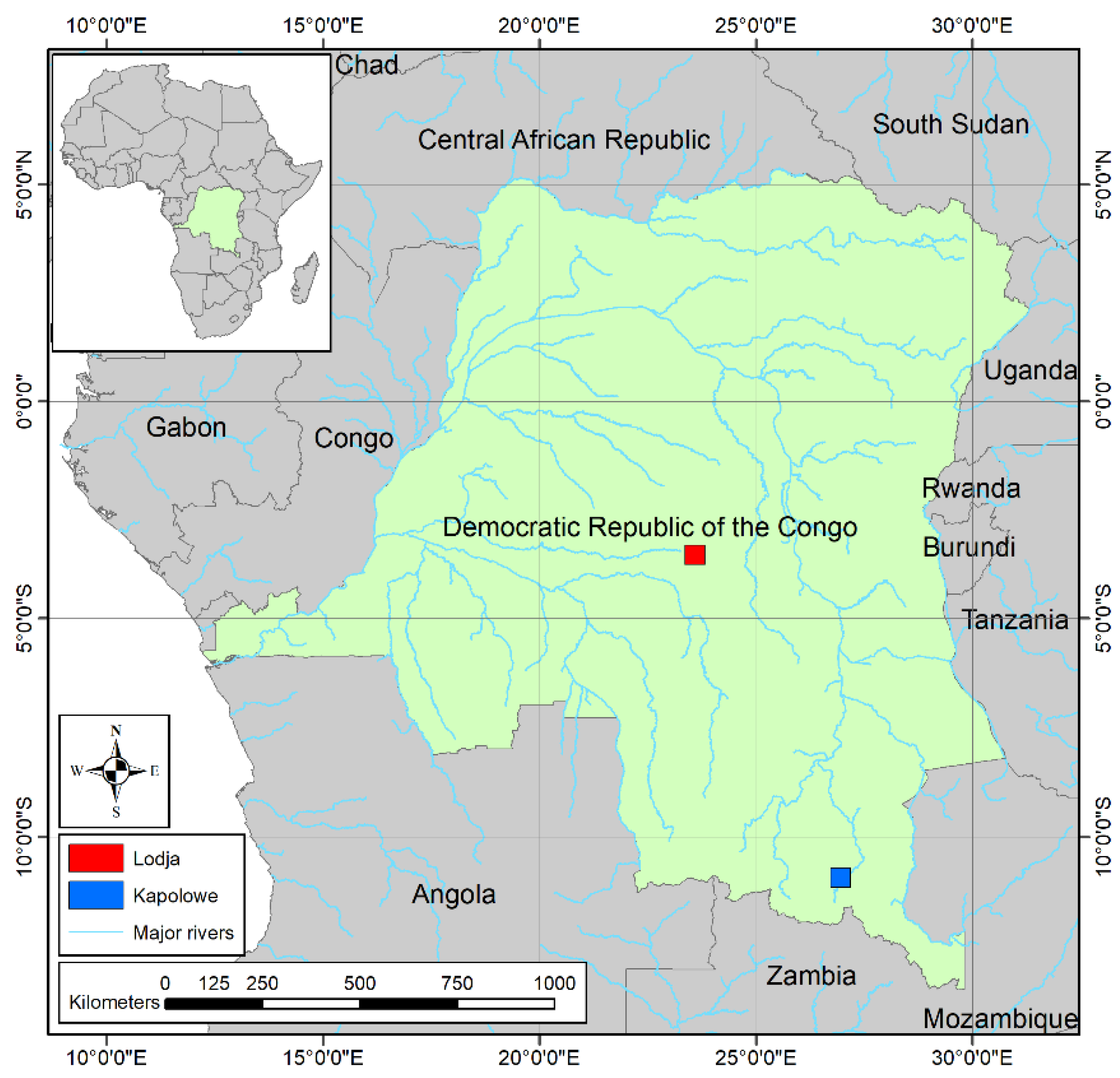
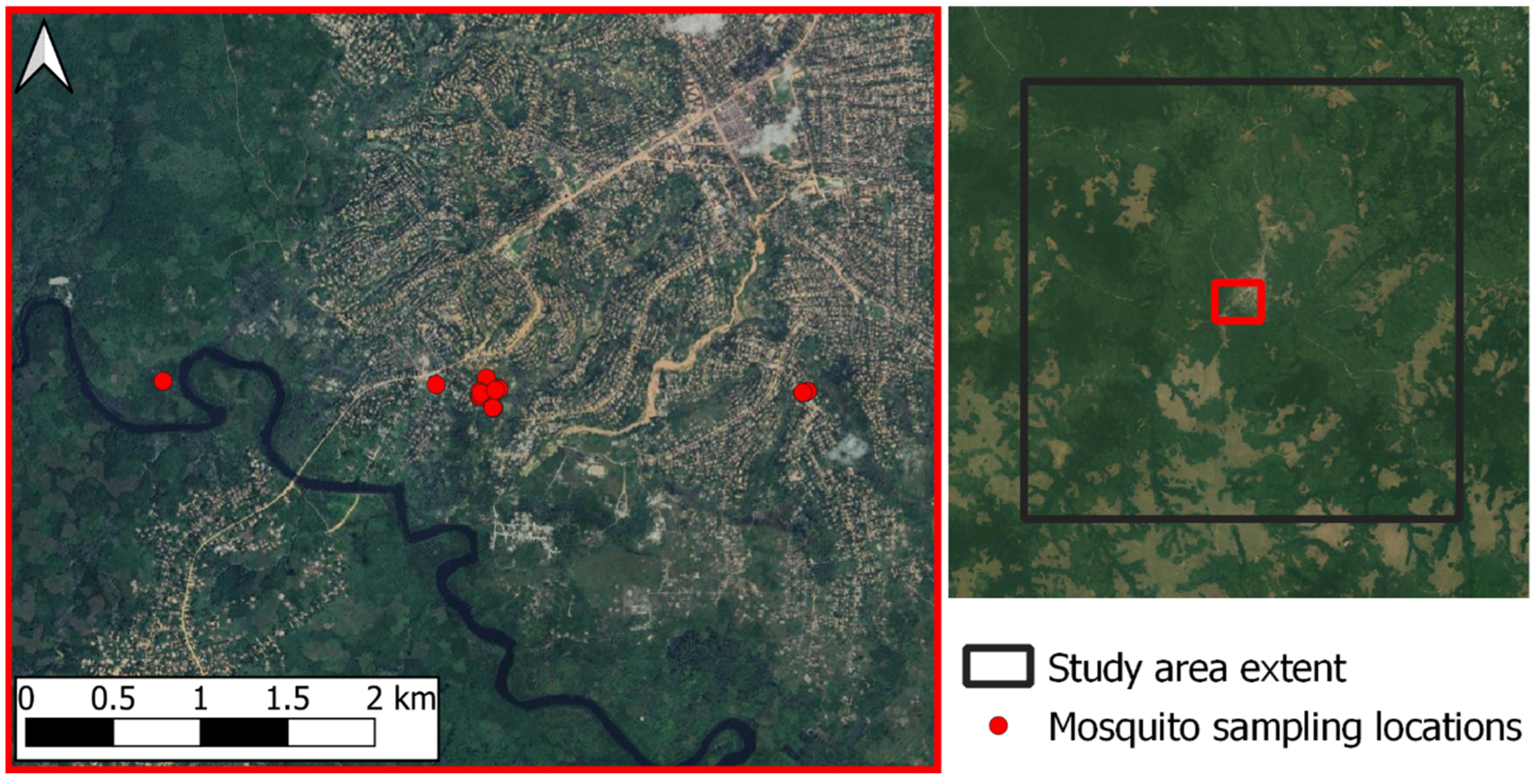
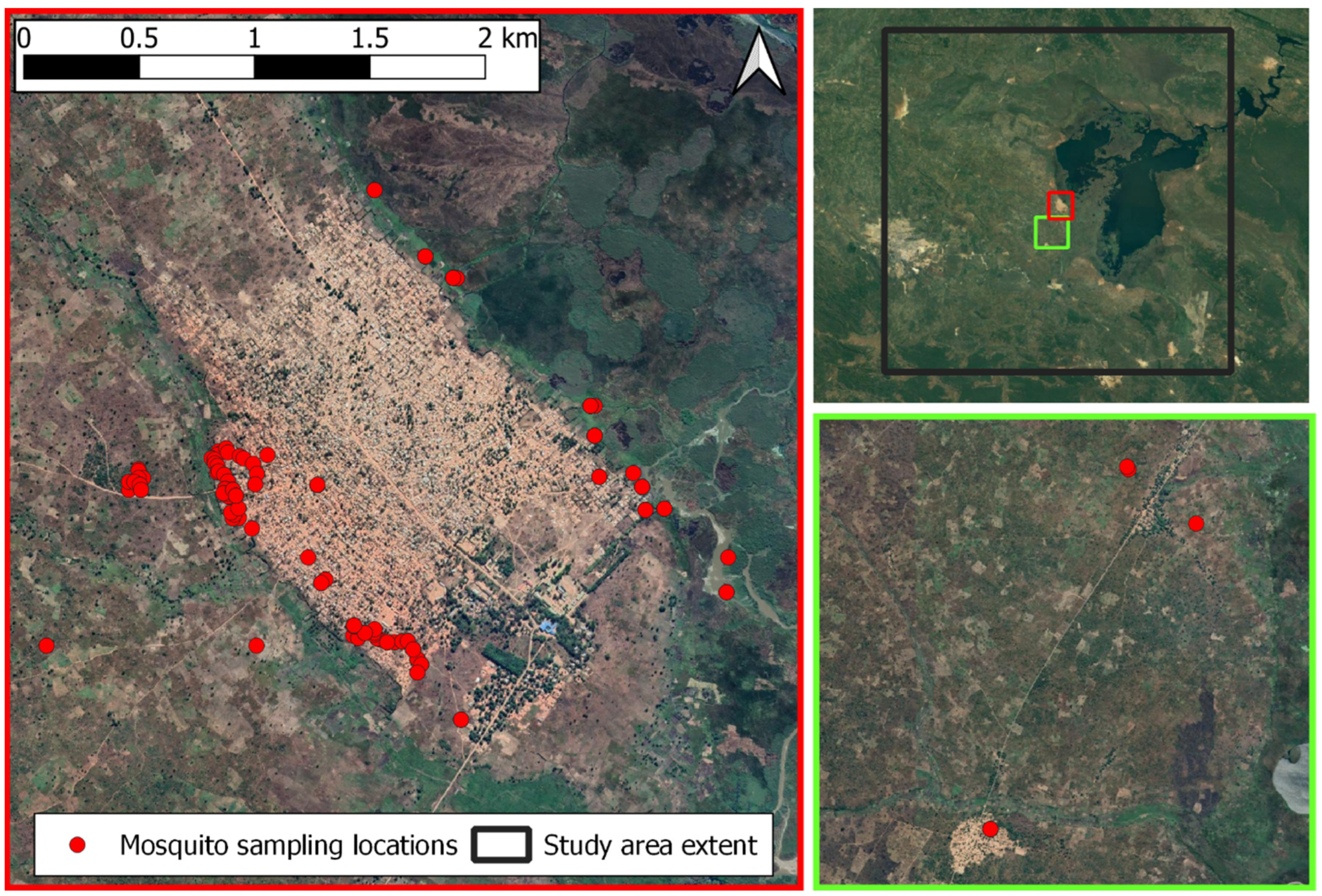
2.1. Study Area

This project focused on two 50 km × 50 km urban areas and their surroundings in the DRC: the medium-sized town of Lodja (population approx. 80,000) (latitude: −3.524661°, longitude: 23.596669°) and a smaller settlement, Kapolowe (latitude: −10.942157°, longitude: 26.952115°) (Figure 1). Both are meso-endemic for malaria, with parasite prevalence between 6 and 30% [46] and with high Plasmodium sporozoite rates for An. gambiae s.l. (Lodja 2.9% (9/307), Kapolowe 6.3% (8/127)) and An. funestus (Lodja 0% (0/24), Kapolowe 8% (4/50)) [47].
The areas surrounding these two towns are typified by a mix of land cover components, including traditional smallholder shifting cultivation (cleared land, active fields, and fallow fields) along with settlements, grassy and bare areas, and a forest interface. The Lukene river flows immediately to the south of Lodja, and the area to the east of Kapolowe is dominated by Lake Tshangalele and large expanses of swamp. At Lodja, mean monthly rainfall (between 1991–2015) was <100 mm for June and July and 100–220 mm/month for the other months of the year, with mean temperatures of 24–26 °C all year round. In Kapolowe, mean monthly rainfall is more seasonal than that of Lodja, with a pronounced dry period between May and September, followed by a rainy season from October to April when the mean rainfall is approximately 30–200 mm/month [47]. The mean temperature in Kapolowe over the year varies more than that of Lodja, ranging from 18 °C in June and July up to 25 °C in October. In 2015, PermaNet 2.0 (deltamethrin) nets were distributed in Lodja, and in 2016, DawaPlus 2.0 (deltamethrin) nets were distributed in Kapolowe. Both distributions were part of provincial distributions. No indoor residual spraying was conducted at either site.

2.2. In Situ Mosquito Data Collection

Mosquitoes were collected monthly by the Institut National de Recherche Biomédicale (INRB, DRC) during 2015–2017 and 2019 in Lodja and 2016–2017 in Kapolowe. Mosquitoes were collected from each of the Lodja and Kapolowe study areas using human landing catches (HLCs), as previously described in [47]. Field technicians undertook eight HLCs over four nights each month, with two different houses each night (total of eight different houses each month). At each house between 18:00 hrs and 06:00 hrs, two technicians conducted indoor HLCs, and two others conducted outdoor HLC. Although focused within the urban areas of Lodja and Kapolowe, the areas surrounding the sampling locations were heterogeneous in terms of land cover present, comprising built-up areas, trees, grassland, fallow areas, static water (fish ponds), and flowing water. Sampling locations at Kapolowe were focused on the edges of or outside the built-up area, in close proximity to a mix of land cover types that are distributed across the wider study area (Figure 2 and Figure 3). Houses were chosen by the collection teams based on proximity to known larval sites, acceptance by households, and other logistical concerns.
In Lodja, a similar proportion of An. gambiae s.l. and An. coluzzii was collected, and species identification for An. gambiae s.l. was not performed for mosquitoes from Kapolowe [47]. An. gambiae s.l. refers to the An. gambiae complex of eight species that are morphologically indistinguishable from each other and that can only be differentiated by molecular analysis [48]. In this study An. gambiae were not identified at the species level; therefore, senus lato (s.l.) was used for the rest of the study. Monthly collection enabled the assessment of the variation in mosquito prevalence in response to current and preceding rainfall and land surface temperature conditions.

2.3. Environmental Variables

A series of biogeographical variables, previously identified as being ecologically relevant to the mosquito life cycle and malaria transmission, were modelled here in relation to mosquito abundance. These include topography, land cover, vegetation index, land surface temperature, and precipitation variables (Table 1).
For this study, all variables were considered to be temporally stable for the time-period of mosquito data collection with the exception of the monthly precipitation and land surface temperature data, which varied each month. Median vegetation index value datasets were generated from all available cloud-free Sentinel-2 imagery, acquired during the mosquito data collection periods for each study area, quantifying the relative ‘typical’ vegetation state across the study areas and the spatial variability thereof.

2.4. Remote Sensing Analysis

2.4.1. Pre-Processing

This study used Google Earth Engine (GEE) as the principal source of remote sensing and environmental data sets and for performing data pre-processing and analysis. The utilized remote sensing datasets were Sentinel-1 (SAR) [52] and Sentinel-2 (optical) data [53], along with Climate Hazards Group InfraRed Precipitation with Station data (CHIRPS) monthly precipitation data [54], MODIS land surface temperature and emissivity data [55], and Shuttle Radar Topography Mission (SRTM) data [56,57] for topographical characterisation. The acquisition dates of the remote sensing datasets covered the period of mosquito data collection for each site.
To generate land cover maps of each study area, Sentinel-1 SAR data and Sentinel-2 optical images were utilised synergistically. The Sentinel-1 SAR data were descending orbit data, with VV and VH polarisations and the derived ratio (VH/VV), from the Ground Range Detected (GRD) data product in the Interferometric Wide Swath (IW) acquisition mode. These data underwent pre-processing (GRD border noise removal, thermal noise removal, radiometric calibration, and orthorectification to derive the backscatter coefficient (Sigma Naught dB) of each pixel) [58]. Median reducers in GEE were used to produce median pixel value composite raster layers from image collections for VV, VH, and VH/VV polarisations from all available data acquisitions in the time periods of 1 January 2016 to 31 December 2019 for Lodja and 1 January 2016 to 31 December 2017 for Kapolowe, prior to subsetting the data to the study area extents. At each location in the output median pixel value composite, the pixel value is the median of all unmasked pixels in the input imagery collection. Median values, derived from a full annual cycle of Sentinel-1 data, were used here to be representative of the general landscape condition throughout the year. This was performed instead of using data from a single date, which, depending on the vegetation phenological stage, may be less representative of the general landscape condition.
The Sentinel-2 (optical) Level 2A orthorectified surface reflectance data at a 10/20 m spatial resolution (depending on spectral band) was used in this study. All available Sentinel-2 images corresponding to the mosquito sampling periods for each site were selected and cloud and cloud-shadow masked using the Sentinel-2 Cloud Probability product, which is also available in GEE. A median pixel value composite image, also produced in GEE using a median reducer, was then generated from the collections of images for each site. For the Sentinel-2 imagery, spectral bands 2 (490 nm), 3 (560 nm), 4 (665 nm), 5 (705 nm), 6 (740 nm), 7 (783 nm), 8 (842 nm), 8a (865 nm), 11 (1610 nm), and 12 (2190 nm) were used. Topographical characterisation of the study areas used 30 m resolution SRTM Digital Elevation Model (DEM) data. Slope and aspect variables were derived from this DEM, with the Topographical Position Index (TPI) calculated as the elevation of the pixel in question, minus the mean elevation of the surrounding 15-pixel radius area.

2.4.2. Land Cover Classification

To perform the land cover classifications, the Sentinel-2 imagery (10 retained bands), the median Sentinel-1 SAR bands (VV, VH, and VH/VV), and the SRTM bands (elevation, aspect, and slope) were composited together to form a 16-band data stack. This data stack was then classified using a Random Forest (RF) classifier with 500 trees. An eight-class classification nomenclature was used specifically targeting land cover types relevant to the ecology of mosquitoes, for example, forests (with woodland edges being important resting areas), water (larval habitats), and built-up areas (with human populations susceptible to malaria infection) (Table 2).
Reference data for both training and validating the land cover classifications were collected from three sources: (1) field collected locations of known land cover classes (with locations recorded via GPS and collected during field mosquito sampling); (2) further reference locations derived from field-collected photographs; and (3) visual interpretations of VHR satellite imagery available through public portals, such as Google Earth and Bing Aerial map layers. The use of higher resolution imagery as reference data is an established technique [41,60], with Google Earth archives also previously being successfully used for this purpose [32,39].
For validation, a regular point grid with 2 km spacing was generated for both study areas, with the land cover at these locations identified via the VHR imagery, ensuring a spread of validation points across the full areas. Additional points were added for sparse and spatially clustered classes to ensure a minimum of 30 validation points were collected for each class (following [32]). An RF classifier was used to generate the land cover classifications using Google Earth Engine. RF classifiers are well established for mapping land cover and have also been used to generate land cover maps within a malaria study context [32]. Accuracy assessments of each land cover classification using the reference validation data were performed, with confusion matrices produced for each study area (Tables S1 and S2).
Proportional coverage (percentage fractional cover) of each land cover class across the study areas was calculated using a moving window to assess whether the increased presence of certain habitats, for example, water serving as a larval habitat, is related to increased mosquito abundance. Additionally, the proportional presence of forest and fallow classes combined was calculated. This was performed independently for each mosquito species, with different kernel sizes used based on established mosquito flight range. Mosquito flight range is species-specific and is influenced by environmental conditions (e.g., wind and vegetation) and physiological status (e.g., sugar or blood fed). The average flight range for An. gambiae is 846 m and for An. funestus is 300 m, with no information available for An. paludis [61]. Maximal flight distances of 3–10 km have also been reported for An. gambiae based on laboratory experiments using flight mills [62]; however, these may not give realistic values compared with field studies [61]. Here, the average flight range for An. gambiae (846 m) was also used for An. paludis. Finally, ‘distance to feature’ raster surfaces were generated, calculating for each pixel the distance from that pixel to the nearest patch of a specific land cover class. This was performed for the forest (i.e., distance to the nearest forest edge), fallow, forest and fallow classes combined, static water, flowing water, and swamp classes.

2.4.3. Vegetation and Water Indices

Two vegetation indices, NDVI [63] and SAVI [64], along with two water indices, NDWI [65] and MNDWI [66], were also calculated. These index values typically vary over time due to phenological and rainfall patterns. A median reducer was applied over the full time periods of mosquito data collection in each site for each of the indices. These median composites represent more ‘typical’ vegetation and water index values over the time period, avoiding the influence that specific or outlying phenological and rainfall patterns could have on single-date images.

2.5. Climatic Data

CHIRPS precipitation data were used to quantify the seasonal precipitation variability, both spatially and temporally, across the mosquito data collection period of the two study areas. The daily CHIRPS product was here converted to a monthly mean product (mean mm/day) for August 2014 to December 2019 for Lodja and for August 2015 to December 2017 for Kapolowe. An additional five months of data prior to the commencement of mosquito data collection was included to assess the influence of rainfall values in the months preceding mosquito data collection. The spatial resolution of these data is 0.05°; however, to avoid artificial pixel-edge boundaries, the data are here smoothed using a 10 km kernel size moving window to generate a smoothed precipitation surface for each month. Each output pixel value corresponds to the mean precipitation value of the kernel area centred on the location of that pixel for that given month. To quantify temporal variability in land surface temperature, MODIS MOD11A1.061 Terra Land Surface Temperature (LST) and Emissivity daily global 1 km data [55] were used to calculate monthly mean LST data sets for the period five months preceding and for the duration of mosquito data collection.

2.6. Random Forest Analysis and Predictive Risk Modelling

The remote-sensing-derived and environmental raster data sets were combined into a single data cube for each 50 km × 50 km study area at a 10 m spatial resolution. The coarser bands (such as the CHIRPS precipitation and MODIS LST data) were effectively resampled to a higher level of detail, with multiple 10 m pixels (of the same value) in the data cube corresponding to a single original CHIRPS or MODIS pixel extent.
The mosquito data were then split into separate calendar month datasets (48 in total for Lodja and 24 for Kapolowe). For each of these, the variables contained as layers in the data cube were extracted. For each month of mosquito data collection, the rainfall values for the current and preceding five months were extracted on a rolling basis and were recorded in a consistent manner (rainfall in current month, rainfall0, rainfall in preceding month, rainfall-1, etc.). Extracted data from all months were then recompiled into species-specific data sets, combining the data from each of the two study areas for each species.
Modelling of the explanatory variables (comprising the topographical variables, land cover class distributions (proportional coverage of individual land cover classes, and the distance to the nearest patch of key land cover type), vegetation indices, and the current and preceding five months of precipitation and LST data) was performed in relation to mosquito abundance data for each mosquito species using RF analysis. Mosquito data from the two study sites were pooled for each species, with correlation plots for the explanatory variables (Table 1) produced (available in Supplementary Information, Figures S1 and S2, which differ slightly due to different species average flight ranges) prior to feature selection being performed to identify and retain a subset of only those variables that were statistically relevant to the mosquito abundance. Given the high correlation between NDVI and SAVI, as shown in the correlation plots, SAVI was disregarded from further analysis. Feature selection used the Boruta method, which implements a feature selection algorithm designed as a wrapper around an RF algorithm [67], and was performed in R (v4.0.3) using the Boruta (v7.0.0; [68]) and randomForest (v4.6.14, [69]) packages.
The Boruta algorithm provides a stable and unbiased selection of important and non-important features by comparing the relevance of the real features to that of random probes [69]. This works by firstly adding randomness to the data set by creating multiple shuffled copies of all features, which are termed as shadow features. It then trains an RF classifier on this extended dataset (including the shadow features) and applies a feature importance measure to evaluate the importance of each feature. In each iteration, this process assesses whether the real feature has a higher importance than its shadow features (whether the feature shows a higher Z score than the maximum Z score of the corresponding shadow features), removing features which are deemed unimportant. The process is repeated until the status of all features is identified as important or unimportant or until a user-defined limit of RF runs is achieved [70]. This process identifies all features that are relevant, either strongly or weakly, to the response variable. This differs from the minimal optimal method of more traditional feature selection methods, which, while producing a minimal set of features and minimising the error of the RF model, can over-prune and discard some relevant variables. The Boruta method of feature selection has been shown to be highly effective and has been recommended above alternative feature selection methods [71].
Once a series of parsimonious variables had been identified by the Boruta feature selection for each of the three mosquito species, each species-specific dataset was split randomly into separate training (80%) and validation (20%) datasets. RFs were used in a regression capacity to model the relationships between mosquito abundance and the parsimonious set of response variables.
RF hyperparameter tuning was performed, with the internal RF parameters (number of trees, minimum leaf population, maximum nodes, number of variables per split, and bag fraction) tuned iteratively to identify the best performing model, determined by the highest R2 value when comparing predicted values to the observed values for the validation data set. For all sites and mosquito species, the RF model parameters that produced the highest R2 values between the predicted and observed values are as follows: number of trees = 200, minimum leaf population = 1, maximum nodes = unlimited, and variables per split = √number of variables. Optimal bag fraction values did vary for each species, with optimal values being 0.7 (An. gambiae s.l.), 0.91 (An. funestus), and 0.6 (An. paludis). RF parameter tuning results are available in Supplementary Information (Tables S3–S5).
With the optimal RF parameters established, each species-specific model was applied predictively [30] for both study areas. All analyses were performed within Google Earth Engine, except for stepwise variable removal using the Boruta method, which was performed in R (v4.2.2, [72]).

2.7. Open Buildings

Open Buildings V1 Polygons data [73], available via Google Earth Engine, were used to identify building footprints within the study areas. This dataset identifies building outlines from 50 cm high-resolution imagery and contains 516 million building detections across 19.4 million km2 of the African continent. Each building has an associated confidence score as a measure of uncertainty that a feature is correctly identified as a building. All buildings with a confidence score of <60% were disregarded, retaining a total of 78,885 and 169,204 buildings for the Lodja and Kapolowe study areas, respectively. For each building, the mean predicted abundance for each species for each month was extracted using zonal statistics in QGIS (v3.28.0).

3. Results

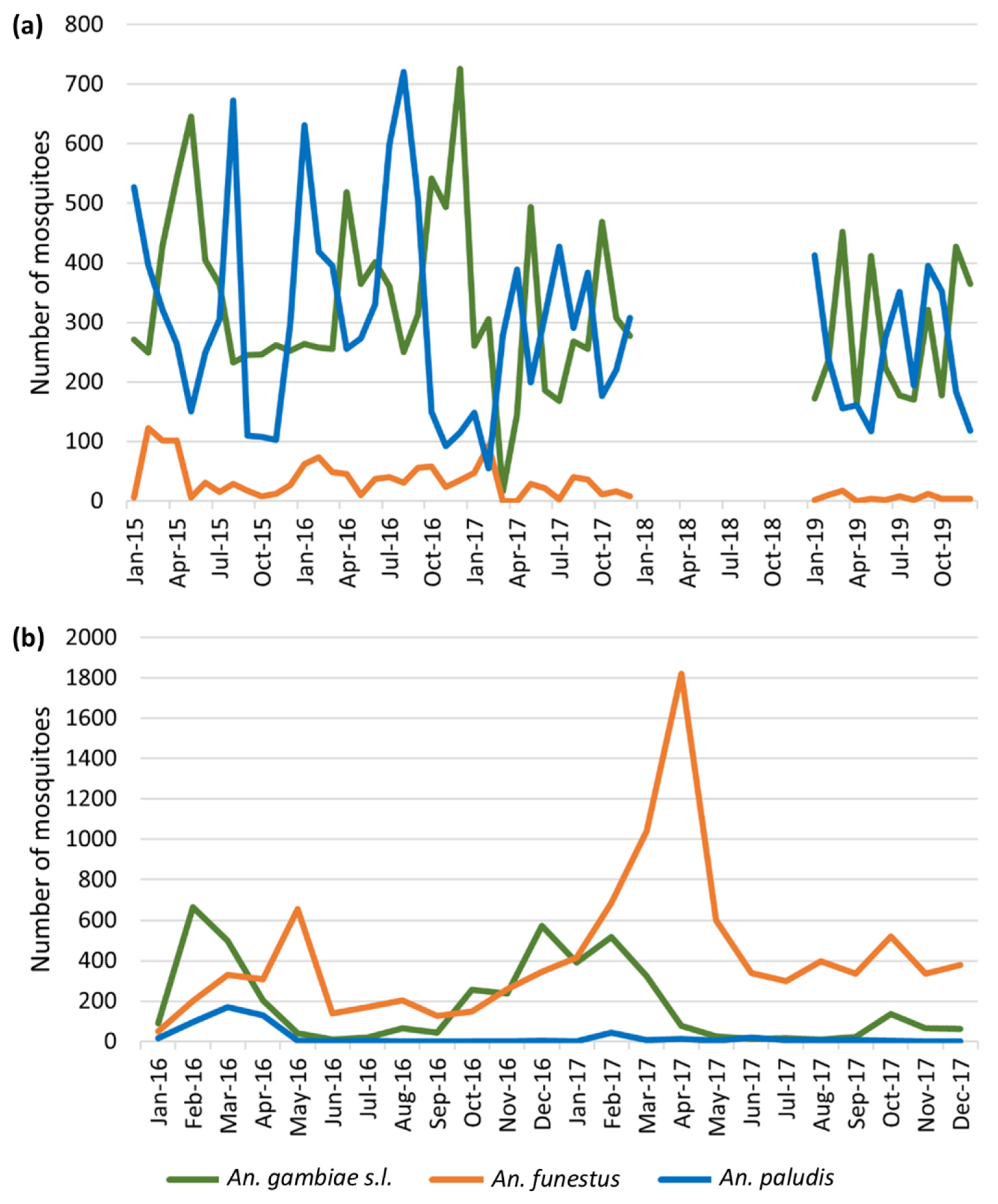
3.1. Mosquito Survey Data

A total of 45,844 mosquito captures were recorded in this study. In Lodja (2015–2019), 49.7% of mosquito collections comprised An. gambiae s.l., followed by An. paludis (43.1%) and An. funestus (5.9%) (Table 3). In Kapolowe (2016–2017), An. gambiae s.l. exhibited lower overall numbers and proportions than those of Lodja (29.0%), with a far higher catch of An. funestus (67.4%), followed by lower catches of An. paludis (3.6%).
For Lodja, An. gambiae s.l. peaked in April-May 2015 and December 2016, whereas An. paludis numbers were greatest in July-August 2015, December-January 2016, and August 2016 (Figure 4). Although far fewer An. funestus were collected in Lodja, the largest counts were collected in January-February 2015 and February 2017. For Kapolowe, An. gambiae s.l. abundance peaked in February-March 2016 and December-March 2017, with the highest counts of An. funestus observed in April 2017. Although fewer An. paludis were collected, the highest capture numbers were observed in February-April 2016.

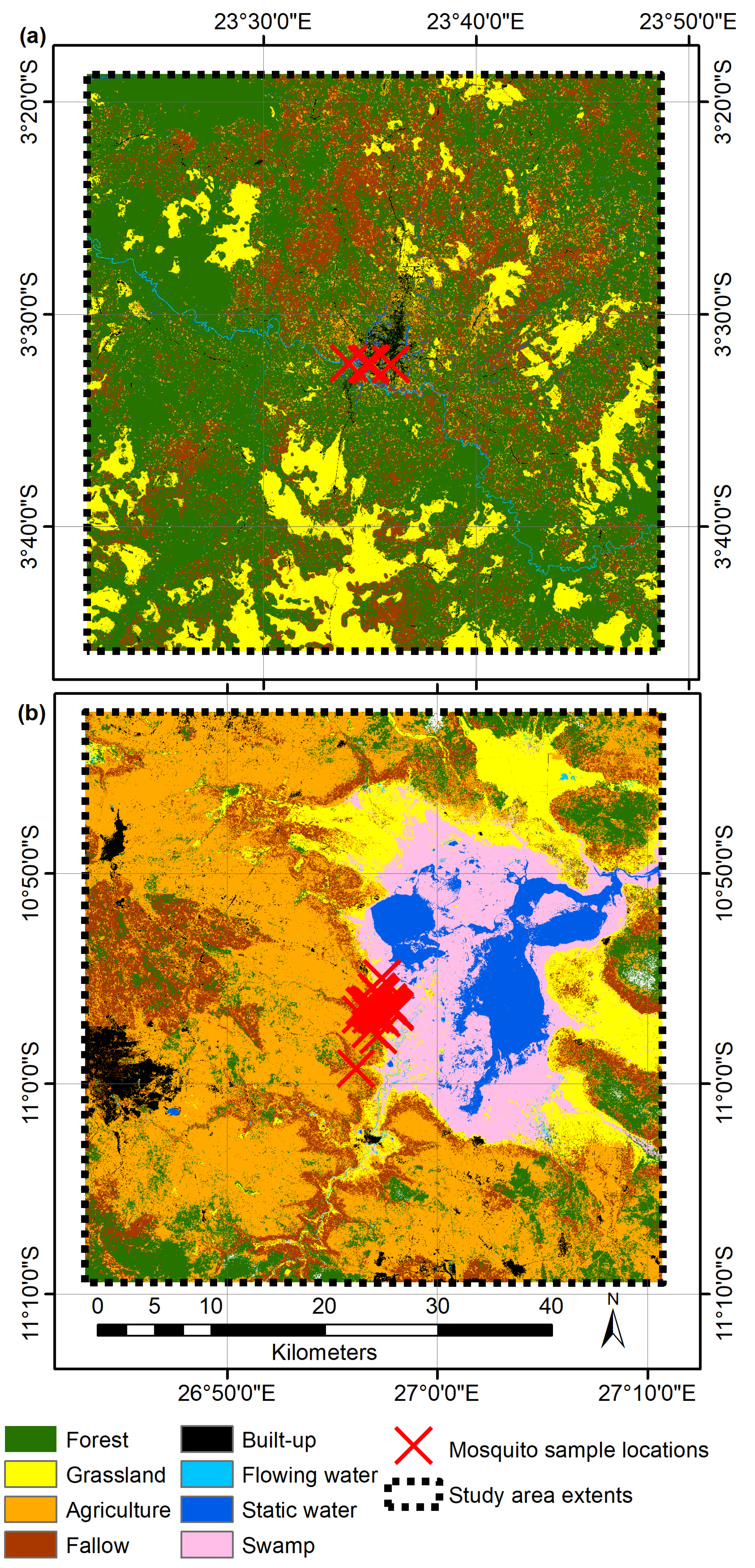
3.2. Land Cover Classification

The land cover classifications successfully characterised the rural complex and wetland areas across the Lodja and Kapolowe study areas (Figure 5), and the land cover class coverages are displayed in Table 4. The overall classification accuracies were 90.60% for Lodja and 90.04% for Kapolowe, and the error matrices are presented in Supplementary Information (Tables S1 and S2).

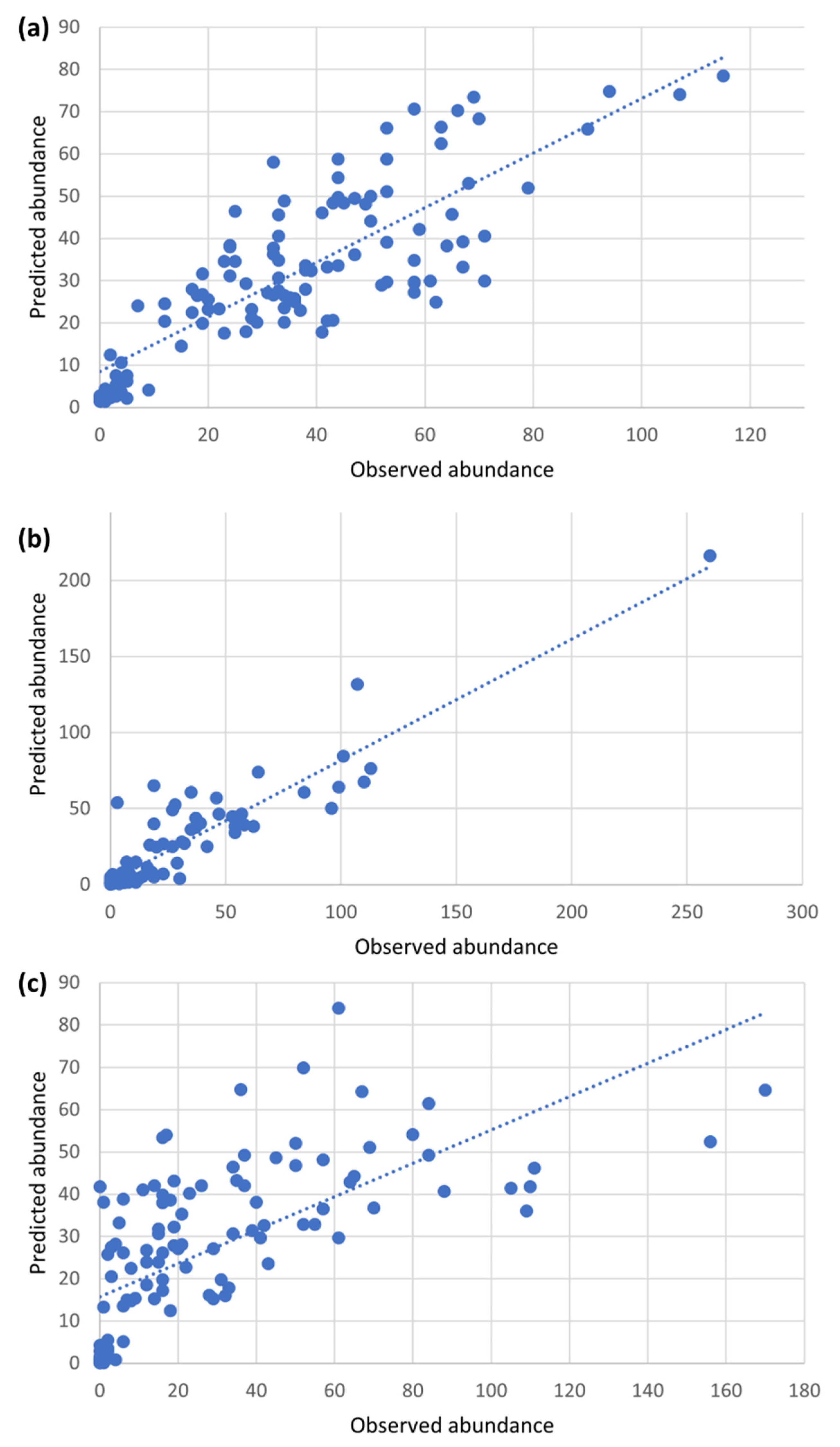
3.3. Random Forest Regression Analysis

The Boruta feature selection of explanatory variables achieved parsimonious models for the abundance of each species, retaining 30 (An. gambiae s.l.), 30 (An. funestus), and 26 (An. paludis) variables for the combined Lodja and Kapolowe data (Table 5). RF regression analysis ranked the relative importance values of the biogeographical variables in relation to An. gambiae s.l., An. funestus, and An. paludis abundance. These importance rankings indicate that, for all species at both sites, the climatic variables of rainfall and land surface temperature (LST) were predominantly identified as being of the highest importance, although the month in relation to mosquito collection (i.e., the month in which a given mosquito sample was collected or any of the preceding five months) varied between species and sites.

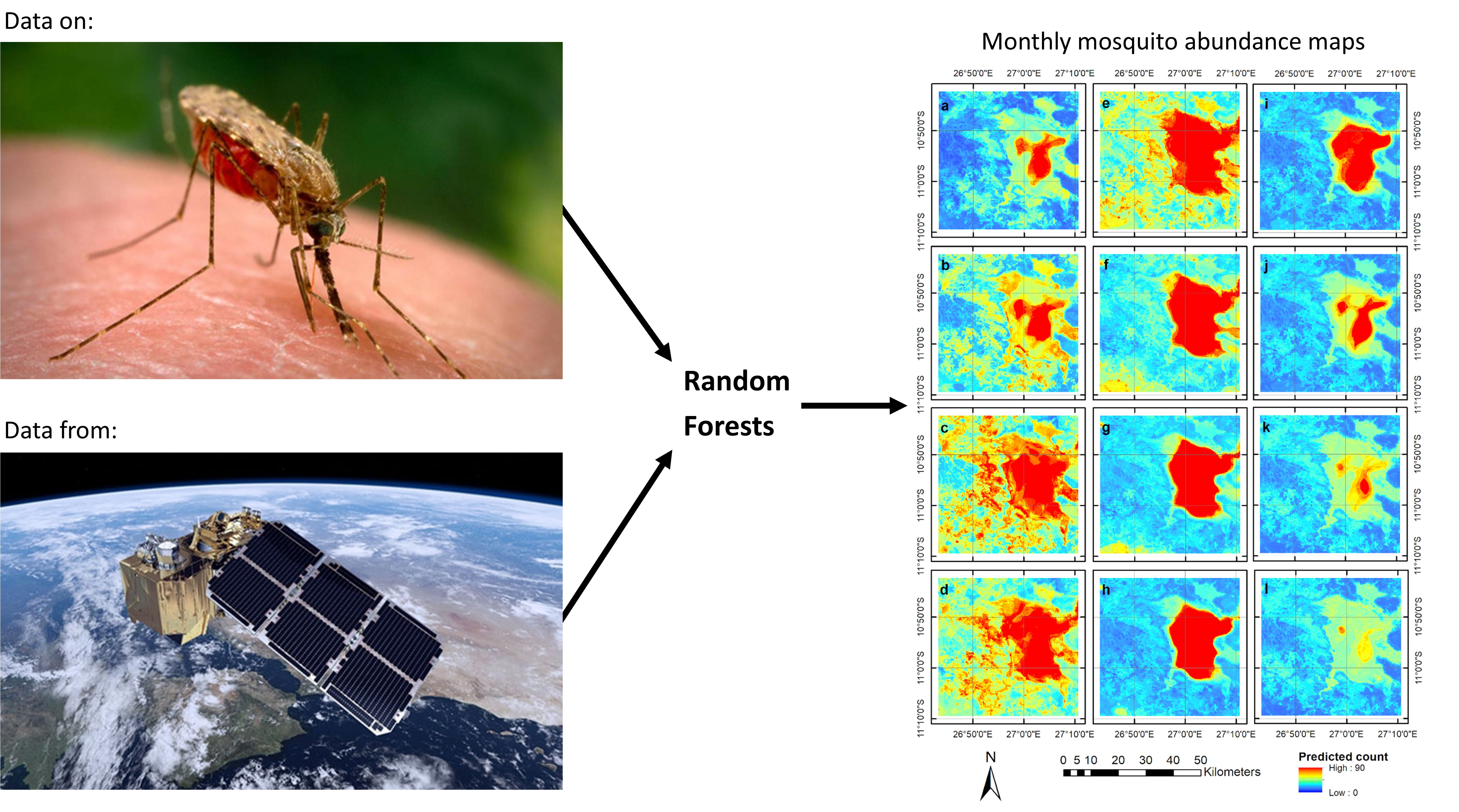
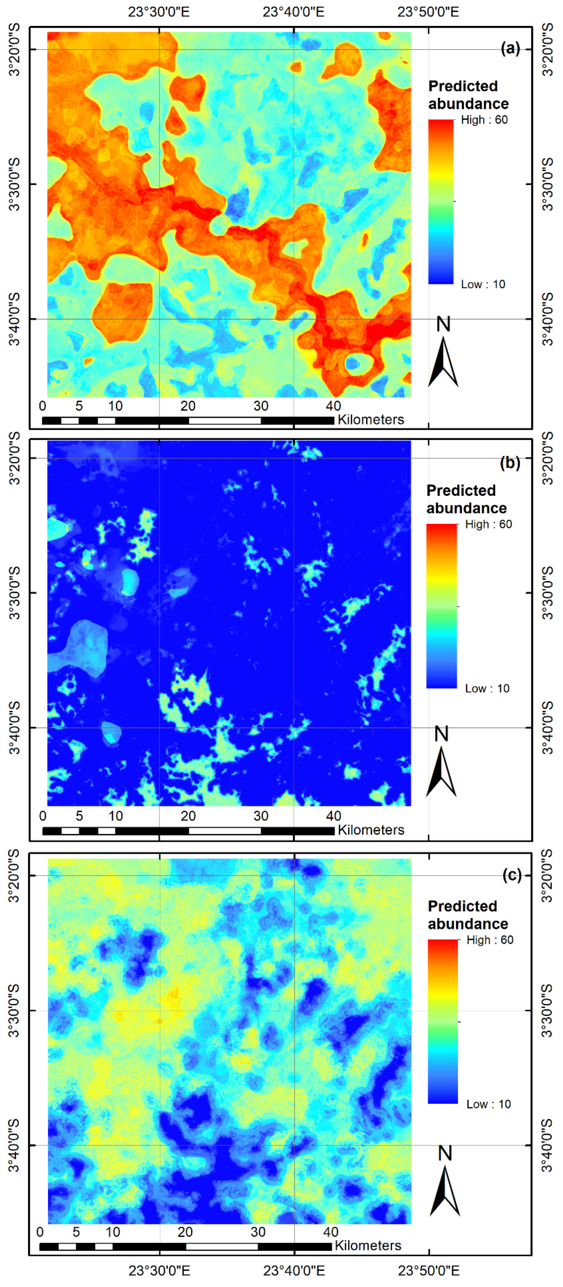
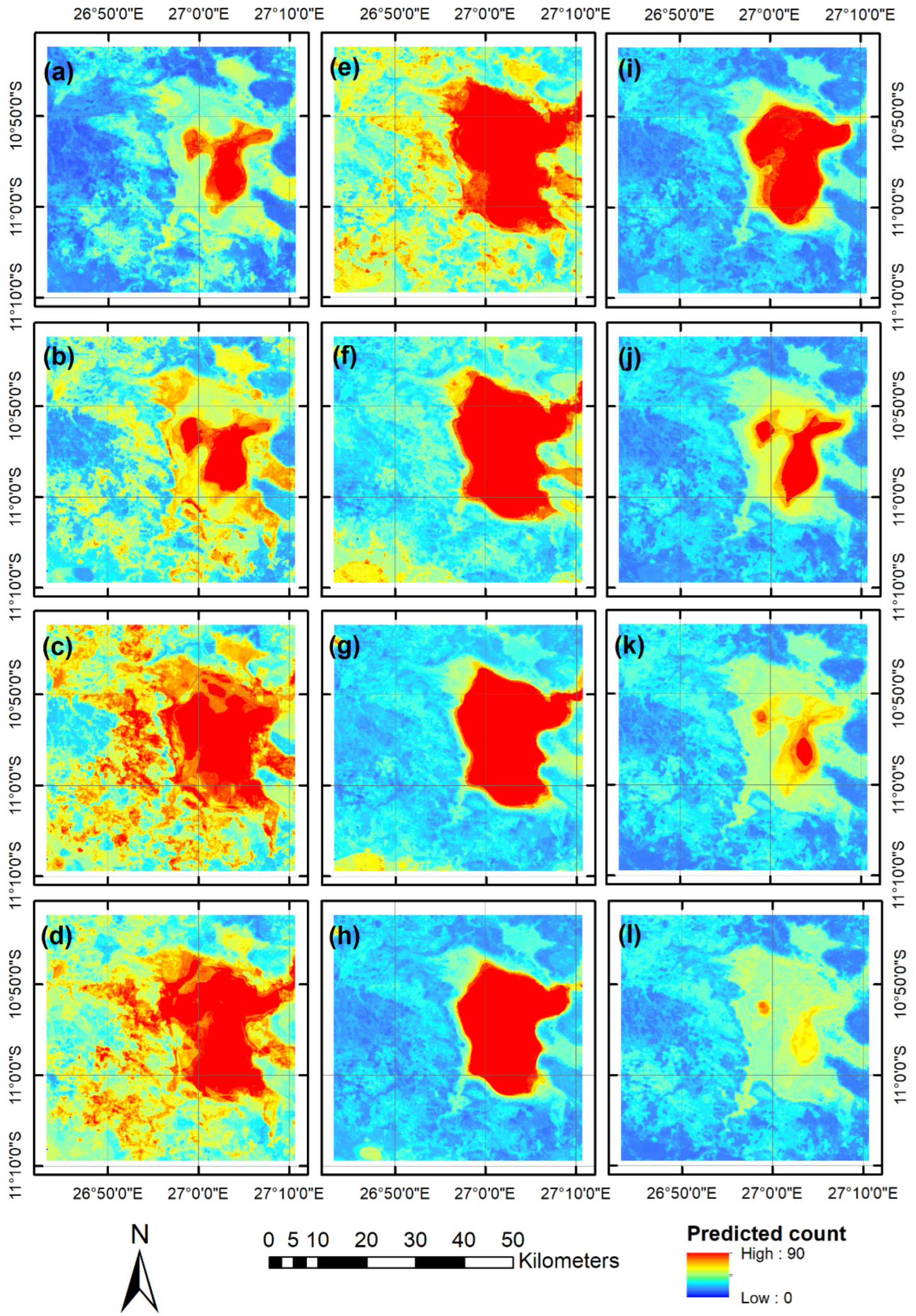
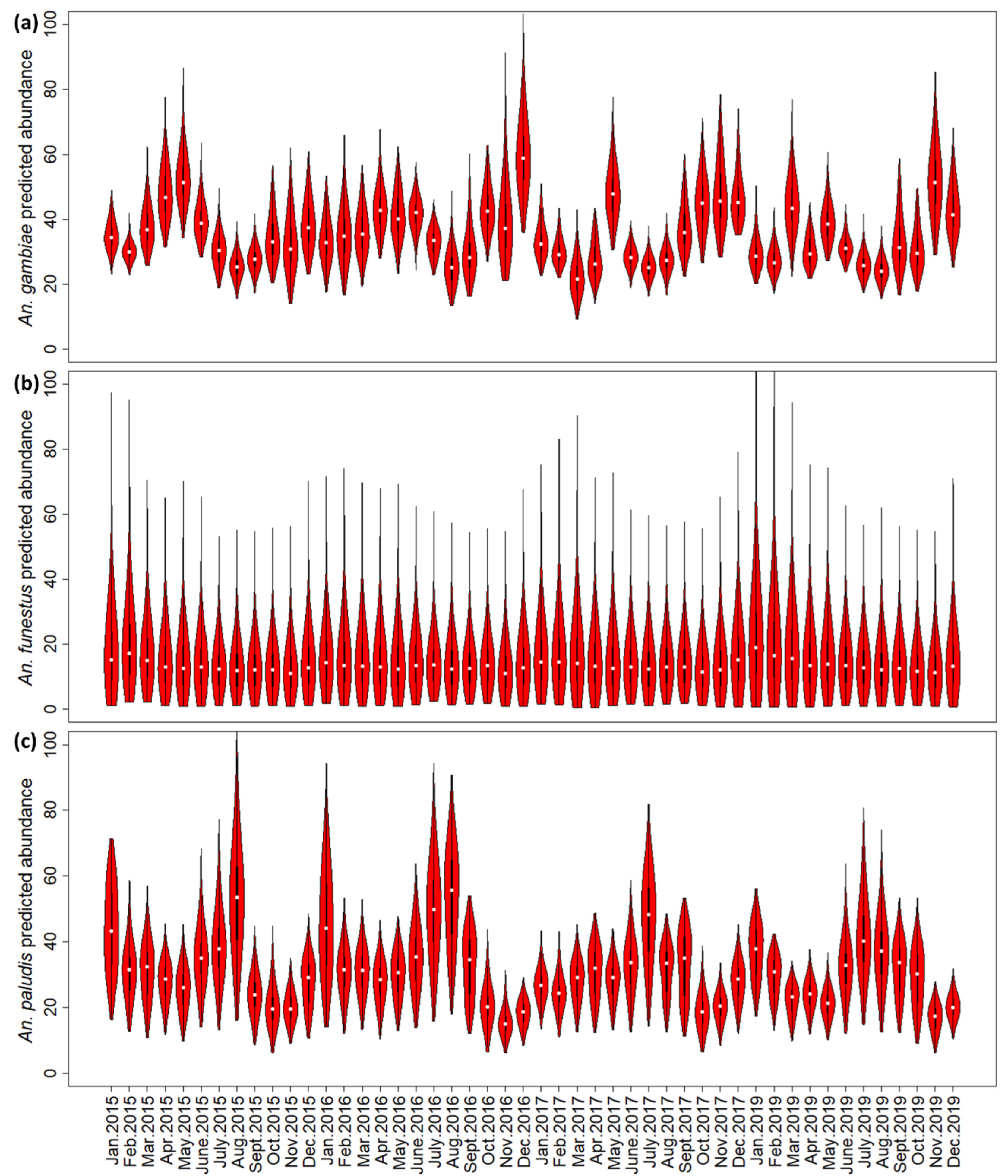
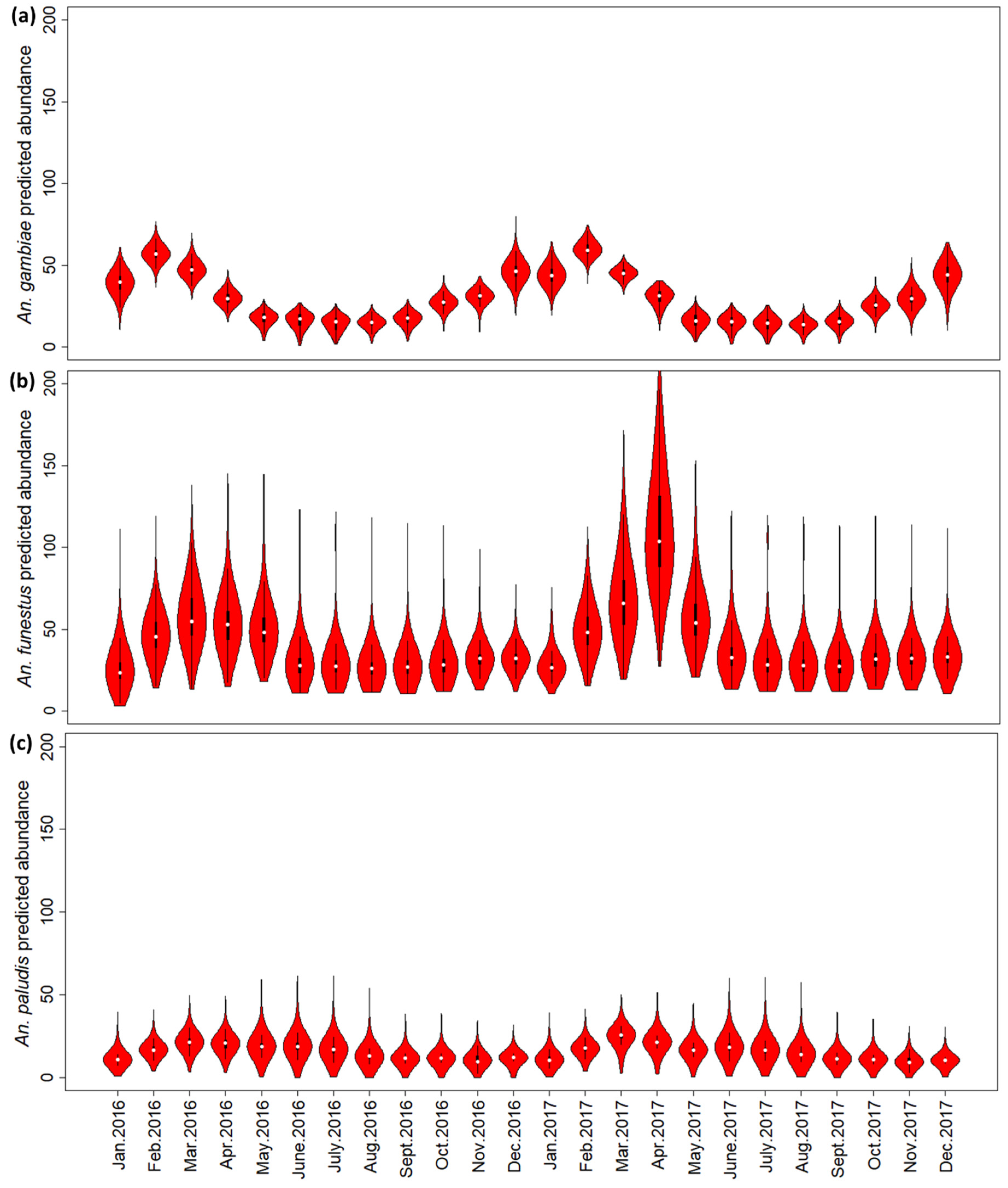
3.4. Predictive Risk Modelling

RF-predicted abundance surfaces were generated for each month and for each mosquito species at the two study sites (January 2015–December 2017 and January 2019–December 2019 for Lodja and January 2016–December 2017 for Kapolowe). The predicted surfaces for all months for all species are presented in Supplementary Information (Figures S3–S20). Specific examples showing the spatial variability in predicted abundance for the three species in Lodja in November 2015 are presented in Figure 6, and Figure 7 shows the seasonal variability in predicted abundances over a year, which here is for An. funestus in Kapolowe in 2016.
An. gambiae s.l. exhibited considerable variability in predicted mosquito abundance, both spatially and temporally, in the Lodja and Kapolowe study areas. Temporal changes in predicted abundances in Lodja broadly followed patterns observed in the field survey data, with peaks consistently occurring in April-May and October-December each year (Figures S3–S6). Spatial variability in predicted abundance was also marked, with areas of higher abundance varying monthly. The highest abundances were observed around the Lukene River and the town of Lodja, for example, in November 2015 (Figure 6) compared with surrounding areas. This could potentially be due to the increased opportunities for pools of water to form/remain in close proximity to the river, and due to the presence of fishponds (static water) found in close proximity to Lodja. Kapolowe also exhibited seasonal variability in predicted An. gambiae s.l. abundance, with lower abundances predicted for May-September in both 2016 and 2017, with higher abundances predicted for other months. The highest predicted abundances occurred in February in both 2016 and 2017 (Figures S7 and S8).
An. funestus exhibited more stable seasonal patterns in predicted abundance for Lodja, with the highest localised abundance peaks occurring in January–May in 2015 and 2019 and in August–September 2016, 2017, and 2019 (Figures S9–S12). Spatially, although predicted abundances for extensive areas remained low, where foci of high abundance did occur, these were typically in areas of open grassland surrounded by forest and in areas of static water, where higher abundances persisted throughout the year. Temporal An. funestus abundance peaks for Kapolowe occurred in February–May in both 2016 and 2017, with generally lower counts observed through the remainder of the year (Figures S13 and S14). Spatially, higher abundances were consistently observed for the Lake Tshangalele area, comprising static water and swamp.
Peaks in An. paludis predicted abundance for Lodja typically occurred in July-August, with broadly lower abundances predicted during the other periods (Figures S15–S18), suggesting that these periods could consistently be periods of high risk for An. paludis in this area, when abundances of An. gambiae s.l. and An. funestus are conversely at their lower levels. Spatially, abundance peaks were distributed across the study area and did not exhibit consistent ties to specific landscape features, although higher peaks were sometimes (such as August 2015 and July–August 2016) observed in close proximity to the town of Lodja. This, along with the Random Forest variable importance rankings (Table 5) is suggestive that abundances are driven principally by rainfall and land surface temperature patterns. For Kapolowe, a higher predicted abundance was generally observed in some sections of the study area from April to June, with broadly lower abundances predicted for all other months (Figures S19 and S20). Spatially, the Lake Tshangalele area generally retains higher predicted abundances than the immediate surrounding area in April-October, although the highest predicted abundances were observed in areas to the east and southwest of the study area with higher levels of forest cover.
The predicted mosquito abundance values were extracted for the locations and times of the validation data, with predicted versus observed abundances compared in a series of scatter plots (Figure 8). This shows a high level of correspondence between the predicted and observed abundance values, with R2 values of 0.707 for An. gambiae s.l., 0.861 for An. funestus, and a lower value of 0.448 for An. paludis.
When peaks of predicted abundance occur in areas of low human population densities, malaria risk may remain low. However, if peaks of mosquito abundance coincide with areas of higher population presence, this can result in increased malaria risk in these communities. To assess the implications for the local community, predicted abundances were extracted for each building, for each species, and for each month. Assessing abundances on a building-by-building basis is valuable, as biting behaviour occurs mostly at night when people are in their homes. Therefore, identifying patterns of risk for individual residences can aid specifically targeting these locations with preventive measures. Figure 9 shows, for a localised area of Kapolowe in February 2017, how An. gambiae s.l. abundance varied considerably over relatively short distances. Buildings on the edge of Kapolowe, which are closer to woodland and arable land cover, exhibited higher abundances than those of more central buildings.
Figure 10 and Figure 11 display the distributions of predicted abundances for each mosquito species for all buildings within Lodja and Kapolowe, respectively, and their change over the duration of the study period. This shows how the predominant species (and therefore biting pressure from those species) differs throughout the study period. For example, Figure 10 shows that, in December 2016, far more buildings had a higher predicted abundance of An. gambiae s.l. than that of An. paludis; however, the opposite was true for July-August 2016. Conversely, An. funestus had a more static profile, reflecting its preference for more permanent water bodies.
The climate and temperature for Kapolowe fluctuate more than they do for Lodja, so the seasonal drop in An. gambiae s.l. numbers in May–September (the dry season) is more pronounced (Figure 11). This shows that a large number of buildings have higher abundances of An. gambiae s.l. during the wet season, with peaks in An. funestus occurring slightly later when An. gambiae s.l. abundances drop, with a particularly high peak in abundance in April 2017. Similar to at Lodja, this demonstrates that different species may be driving biting pressure at buildings at different locations and time periods. An. paludis exhibited a more stable profile at Kapolowe; however, it did exhibit a very high peak abundance for a large number of buildings in April 2017.

4. Discussion

In this study, cost-free multi-temporal remote sensing data, Google Earth Engine, and in situ mosquito sampling data were utilised to identify variables influencing the distribution and abundance of three mosquito malaria transmission vectors and the relative importance of their association. This research, which would not have been possible using ground-based surveys alone, advances the understanding of how environmental dynamics in the study regions influence the distributions of these mosquitos, and it provides risk maps predicting seasonal hot-spots of mosquito abundance in this highly endemic malaria region in the DRC.

4.1. Identifying Spatio-Temporal Drivers of Malaria Risk

Our first objective, to identify the key variables driving Anopheles mosquito species distribution and abundance, can be answered from our analysis. The distributions of An. gambiae s.l., An. funestus, and An. paludis are, in the Lodja and Kapolowe study areas, related to a number of biogeographical variables, but amongst these, principally, is a strong association with rainfall and land surface temperature. Previous studies have demonstrated that the amount and seasonality of rainfall in sub-tropical Africa drastically affect the occurrence and productivity of mosquito larval habitats, limiting the distribution of certain Anopheles species [8]. Rainfall is of particular importance, as higher rainfall generates more larval sites, particularly for species such as An. gambiae s.l., which rely on temporary pools for larval habitats. With the onset of higher rainfall, it follows that mosquito abundance increases. The time it takes from an egg to become adult is around 10–11 days [74], so mosquito numbers are expected to be higher if increased rainfall occurs during both the month in which mosquitos are sampled and during the preceding month, as was observed here for An. gambiae s.l. and An. paludis. An. funestus preferentially exploits permanent water bodies and is therefore less vulnerable to short-term fluctuations in rainfall. It should be noted that other previous studies, such as [75], did not find rainfall to be important. While conducting continental-scale species distribution modelling of An. gambiae, [75] found that temperature and vegetation (characterised by annual NDVI and NDVI variability) were important predictors but that precipitation was not, suggesting that their analysis shows this because rainfall can be highly correlated with other variables that characterise the aridity gradient.
Land surface temperature influences both mosquito abundance and malaria incidence. In general, African malaria vectors are most suited to a temperature range of 13–35 °C [76,77]. Land surface temperature, for example, was shown to be the main environmental variable driving malaria vector abundance in Ethiopia [78]. Temperature also influences the extrinsic incubation period of parasite development in the mosquito, which is a key factor in malaria transmission [79]. Land surface temperature has been shown to be a strong predictor of the deadliest and most common form of human malaria, Plasmodium falciparum [80].
Although rainfall is crucial for providing larval sites, the factors driving mosquito abundance are complex, and other factors are simultaneously at play, for example, vegetation, slope, and soil percolation, which vary in each area. Changes in development time from immature aquatic stages to adults can also be affected by several factors. In laboratory studies, temperature is known to influence developmental time and subsequent larvae and adult survival [81], but it can also influence larval competition in water pools, potentially leading to smaller adults and in turn affecting adult survival [82]. Furthermore, within a single egg batch, early and late hatching was reported with increasing development times for late hatches [83]. Late hatching is believed to be an adaptive strategy for dealing with unstable larval sites (e.g., desiccation) and competition. Although rainfall is identified here as a key variable influencing the abundance of all three mosquito species, other variables are also influential. For example, both the proportional cover of and the distance to forests and fallow was found to be of high importance for An. gambiae s.l., An. funestus, and An. paludis. This was also reported for other Anopheles species [84], with forest edges providing refugia and non-human hosts for feeding.

4.2. Spatio-Temporal Risk Maps

The second objective was to predictively model mosquito distributions and their seasonal variability, and here, both spatial and temporal variability in predicted mosquito abundance for all three mosquito species is demonstrated. The predicted abundance maps illustrate the importance of considering temporal variables, such as seasonal rainfall and land surface temperature patterns, in addition to temporally static variables. Here, seasonal rainfall and land surface temperature are both identified as key drivers of mosquito abundance, resulting in clear variability in predicted abundances throughout the year in response to these variables. By improving the capability of identifying seasonal hot-spots of mosquito abundance, the improved targeting (both of specific localised areas of high risk and of high-risk periods during the year) of intervention measures, such as larval source management (LSM), is possible. Given increasing insecticide resistance and the resulting reduction in effectiveness of some intervention methods (theorised to contribute to the increase of five million recorded cases in 2016 compared with 2015 [3]), LSM interventions may become increasingly important for wide-scale malaria control. In many malaria-endemic regions, disease control activities and monitoring over large geographical areas are exceptionally challenging for resource-constrained nations, such as the DRC, where a large proportion of mosquito-borne disease cases are found but where monitoring cannot currently be performed.
The response to getting the targets of the GTS back on track has been the ‘High Burden to High Impact’ (HBHI) initiative led by the WHO and Roll Back Malaria partnership [85]. This strategy has been adopted by high-burden countries and is underpinned amongst other factors by more timely and granular data that can be used to inform how limited resources can be used for maximum impact and that can improve targeted policies to empower countries to tailor the optimal mix of tools for a range of settings and engagement with sectors beyond health. The approach we used in this study, therefore, fits neatly with the HBHI initiative. By applying methods such as those presented here, high-risk areas, down to the individual building level, can be identified in a cost-effective manner, enabling the prioritisation of high-risk target regions for surveillance, monitoring, and treatment [8], thus shrinking the geographical extents that need targeting in control activities. This can, in turn, make an important contribution towards reducing morbidity and mortality from this preventative disease in the DRC, and it can have a greater impact on reducing malaria infection rates in children under the age of five, for whom the majority of deaths from malaria are recorded. As such, it is of particular use for policy makers in developing effective regional frameworks for malaria control and eradication [35], in line with the HBHI. The value of utilising malaria vector risk maps for intervention decision making was demonstrated in Zambia. Prioritising communities to receive indoor residual spraying (IRS) based on the predictive probabilities of An. funestus led to the greatest decrease in malaria, compared with concentrating IRS within a geographical area or prioritising IRS to communities based on observed malaria incidence [86]. It is possible that a similar approach could be adopted for other interventions.
Given that the mosquito species in this study bite in the evening, the type of a building can influence risk. A building that is identified as high-risk based on mosquito abundance may have less of a malaria risk if it is unoccupied during the evening, e.g., an industrial or commercial building. A second consideration is house structure, which can also influence malaria risk [87]. It was beyond the scope of this current study to determine these two points, but they will be factored into future mapping.

4.3. Transferability of the Method

This method was designed to be transferable to enable wide uptake by practitioners in the field. To accompany this manuscript, a user manual was developed in multiple languages (English, French, and Spanish) and was made openly available (https://doi.org/10.5281/zenodo.6973662, accessed on 1 August 2022), designed to provide non-specialists with step-by-step instructions, thus enabling independent implementation of these methods and avoiding reliance on external specialists [45]. By removing this limitation and empowering local disease control agencies to integrate Earth observation methods as a core element in their activities, it can enable them to independently generate frequent maps of predicted mosquito abundances and distributions for user-defined time periods and study areas as raster data products. This can enable the identification of hot-spots of mosquito abundance—and therefore of potentially increased malaria transmission risk—both spatially and seasonally, allowing more specific targeting by disease control activities to concentrate on areas of the highest risk. As such, it is hoped that significant improvements can be made in targeting resource-constrained disease control programmes, reducing the burden of disease in malaria-endemic areas. Although the methodological framework presented is transferable, it does require input data from the local study areas in question to build site-specific predictive models. Although the utilized EO datasets are available globally via Google Earth Engine, in situ longitudinal mosquito data collection for the study areas of interest (here, collected monthly) from multiple locations within the study areas are required. These data must be collected over at least one year to enable variability in mosquito abundance to be related to temporally dynamic variables, such as annual rainfall patterns. Appropriate training and validation locations for conducting the land cover mapping stage of the analysis are also required. If these datasets are available, the presented methods should be implementable across other malaria-endemic regions and for other relevant mosquito species.

4.4. Future Development

This study identifies the key variables influencing mosquito distributions and abundance in the Lodja and Kapolowe study areas; however, the limited sample size of mosquito survey locations is acknowledged. Although predicted abundance maps for all three species at the two study sites were generated, and although the validation for the observed versus predicted abundance produced strong levels of correspondence, future work should look to expand the number of mosquito sampling locations, increasing their geographical spread and the longitudinal time period over which they are collected. There is limited understanding of the taxonomy of secondary African malaria vectors, as recent work has revealed ambiguous species identification of An. paludis samples, which are now subject to further genetic analysis. Host population abundance was not considered in this study with regarding malaria risk but could be factored into future work.
Further work could also usefully assess the transferability of these methods to different malaria-endemic areas and other mosquito species. This can enable the testing of different modelling methods at different locations to compare the accuracy, ease of application, transparency, and transferability between sites of different methods, which can progress towards the development of a more generic framework approach to modelling mosquito abundance using remote sensing datasets.
Additionally, the spatial resolution of the remote sensing datasets used here (10 m Sentinel 1 and 2 data) may preclude the detection of small water features, which could act as mosquito larval habitats, including features under tree cover. Evidence does, however, suggest that, in sub-Saharan Africa, water bodies under trees are not productive Anopheles habitats, with mosquitoes often preferring sunlit pools for larval habitats [7], potentially reducing the influence of these features. Future studies could additionally conduct drone-based surveys at higher levels of resolution to identify these features and to inform the extent to which the current method is detecting them. Further longer-term studies could also test the hypothesis that certain wetlands can act as refugia for mosquitoes (and therefore also for malaria transmission) during the dry season [32,88], serving as reservoirs for mosquitoes and facilitating the expansion of malaria transmission through the broader region in the wet season [19,32]. This potentially includes sites such as fish ponds, which are present close to Lodja, and permanent wetlands near Kapolowe. Sites such as these, once identified, could be ideal targets for the application of larval source management activities.

5. Conclusions

This study confirms the potential of cost-free remote sensing data, Google Earth Engine, and Random Forests to generate temporally repeatable predictive models of mosquito distribution and abundance over broad study areas to the individual building level. Although demonstrated here on a regional level, the computational capacity of Google Earth Engine offers opportunities for applying these methods to many different regions via cloud computing given suitable in situ data. This overcomes a major challenge in many malaria-endemic regions, where resource constraints inhibit broad-scale ground-based monitoring, and where cost and infrastructure requirements have historically limited the uptake of monitoring via remote sensing. Although the potential of such methods are often recognised, accessibility to and the practical application of these methods are often limited by a lack of Earth observation specialist knowledge. The development of the training materials describing the implementation of the methods described in this article can overcome this reliance on EO specialist knowledge, which historically may have limited the use of EO analysis in malaria programmes. By providing users with the means to implement these methods independently within the context of their own programmes, EO could play an increasingly significant role in informing malaria disease control activities globally, improving the targeting of disease control activities and reducing the burden of this disease in malaria-endemic regions.

Supplementary Materials

The following are available online at https://www.mdpi.com/article/10.3390/rs15010043/s1: Figure S1: Variable correlation plot for An. gambiae and An. paludis; Figure S2: Variable correlation plot for An. funestus; Table S1: Confusion matrix for the Lodja land cover classification; Table S2. Confusion matrix for the Kapolowe land cover classification; Table S3: Random forest parameter tuning for An. gambiae s.l.; Table S4. Random forest parameter tuning for An. Funestus; Table S5: Random forest parameter tuning for An. paludis; Figure S3: Predicted counts of An. gambiae s.l. for the Lodja study area for (a) January 2015; (b) February 2015; (c) March 2015; (d) April 2015; (e) May 2015; (f) June 2015; (g) July 2015, (h) August 2015; (i) September 2015; (j) October 2015; (k) November 2015; (l) December 2015; Figure S4: Predicted counts of An. gambiae s.l. for the Lodja study area for (a) January 2016; (b) February 2016; (c) March 2016; (d) April 2016; (e) May 2016; (f) June 2016; (g) July 2016, (h) August 2016; (i) September 2016; (j) October 2016; (k) November 2016; (l) December 2016; Figure S5: Predicted counts of An. gambiae s.l. for the Lodja study area for (a) January 2017; (b) February 2017; (c) March 2017; (d) April 2017; (e) May 2017; (f) June 2017; (g) July 2017, (h) August 2017; (i) September 2017; (j) October 2017; (k) November 2017; (l) December 2017; Figure S6: Predicted counts of An. gambiae s.l. for the Lodja study area for (a) January 2019; (b) February 2019; (c) March 2019; (d) April 2019; (e) May 2019; (f) June 2019; (g) July 2019, (h) August 2019; (i) September 2019; (j) October 2019; (k) November 2019; (l) December 2019; Figure S7: Predicted counts of An. gambiae s.l. for the Kapolowe study area for (a) January 2016; (b) February 2016; (c) March 2016; (d) April 2016; (e) May 2016; (f) June 2016; (g) July 2016, (h) August 2016; (i) September 2016; (j) October 2016; (k) November 2016; (l) December 2016; Figure S8: Predicted counts of An. gambiae s.l. for the Kapolowe study area for (a) January 2017; (b) February 2017; (c) March 2017; (d) April 2017; (e) May 2017; (f) June 2017; (g) July 2017, (h) August 2017; (i) September 2017; (j) October 2017; (k) November 2017; (l) December 2017; Figure S9: Predicted counts of An. funestus for the Lodja study area for (a) January 2015; (b) February 2015; (c) March 2015; (d) April 2015; (e) May 2015; (f) June 2015; (g) July 2015, (h) August 2015; (i) September 2015; (j) October 2015; (k) November 2015; (l) December 2015; Figure S10: Predicted counts of An. funestus for the Lodja study area for (a) January 2016; (b) February 2016; (c) March 2016; (d) April 2016; (e) May 2016; (f) June 2016; (g) July 2016, (h) August 2016; (i) September 2016; (j) October 2016; (k) November 2016; (l) December 2016; Figure S11: Predicted counts of An. funestus for the Lodja study area for (a) January 2017; (b) February 2017; (c) March 2017; (d) April 2017; (e) May 2017; (f) June 2017; (g) July 2017, (h) August 2017; (i) September 2017; (j) October 2017; (k) November 2017; (l) December 2017; Figure S12: Predicted counts of An. funestus for the Lodja study area for (a) January 2019; (b) February 2019; (c) March 2019; (d) April 2019; (e) May 2019; (f) June 2019; (g) July 2019, (h) August 2019; (i) September 2019; (j) October 2019; (k) November 2019; (l) December 2019; Figure S13: Predicted counts of An. funestus for the Kapolowe study area for (a) January 2016; (b) February 2016; (c) March 2016; (d) April 2016; (e) May 2016; (f) June 2016; (g) July 2016, (h) August 2016; (i) September 2016; (j) October 2016; (k) November 2016; (l) December 2016; Figure S14: Predicted counts of An. funestus for the Kapolowe study area for (a) January 2017; (b) February 2017; (c) March 2017; (d) April 2017; (e) May 2017; (f) June 2017; (g) July 2017, (h) August 2017; (i) September 2017; (j) October 2017; (k) November 2017; (l) December 2017; Figure S15: Predicted counts of An. paludis for the Lodja study area for (a) January 2015; (b) February 2015; (c) March 2015; (d) April 2015; (e) May 2015; (f) June 2015; (g) July 2015, (h) August 2015; (i) September 2015; (j) October 2015; (k) November 2015; (l) December 2015; Figure S16: Predicted counts of An. paludis for the Lodja study area for (a) January 2016; (b) February 2016; (c) March 2016; (d) April 2016; (e) May 2016; (f) June 2016; (g) July 2016, (h) August 2016; (i) September 2016; (j) October 2016; (k) November 2016; (l) December 2016; Figure S17: Predicted counts of An. paludis for the Lodja study area for (a) January 2017; (b) February 2017; (c) March 2017; (d) April 2017; (e) May 2017; (f) June 2017; (g) July 2017, (h) August 2017; (i) September 2017; (j) October 2017; (k) November 2017; (l) December 2017; Figure S18: Predicted counts of An. paludis for the Lodja study area for (a) January 2019; (b) February 2019; (c) March 2019; (d) April 2019; (e) May 2019; (f) June 2019; (g) July 2019, (h) August 2019; (i) September 2019; (j) October 2019; (k) November 2019; (l) December 2019; Figure S19: Predicted counts of An. paludis for the Kapolowe study area for (a) January 2016; (b) February 2016; (c) March 2016; (d) April 2016; (e) May 2016; (f) June 2016; (g) July 2016, (h) August 2016; (i) September 2016; (j) October 2016; (k) November 2016; (l) December 2016; Figure S20: Predicted counts of An. paludis for the Kapolowe study area for (a) January 2017; (b) February 2017; (c) March 2017; (d) April 2017; (e) May 2017; (f) June 2017; (g) July 2017, (h) August 2017; (i) September 2017; (j) October 2017; (k) November 2017; (l) December 2017.

Author Contributions

Conceptualisation, C.M., C.S. and C.R.; methodology, C.M., C.S. and C.R.; formal analysis, C.M., C.S. and C.R.; investigation, C.M., C.S. and C.R.; data curation, C.M., S.I., F.W. and C.S.; writing—original draft preparation, C.M., C.S., S.I., C.R. and P.A.; writing—review and editing, C.M., C.S., S.I., C.R., A.O., P.G., P.M.-G. and P.A.; visualisation, C.M.; funding acquisition, C.M., C.S., S.I. and P.A. All authors have read and agreed to the published version of the manuscript.

Funding

This project was funded through a UKRI Collective Fund administered by Edge Hill University as part of the Global Challenges Research Fund, the UK Centre for Ecology and Hydrology (project number NEC07217); and the Natural Environment Research Council (Grant number NE/R016429/1 as part of the UK-SCAPE programme delivering National Capability). Seth Irish was supported by the U.S. President’s Malaria Initiative. The findings and conclusions in this paper are those of the authors and do not necessarily represent the official position of the Centers for Disease Control (CDC).

Institutional Review Board Statement

The study was conducted in accordance with the Declaration of Helsinki, and approved by the Institutional Review Board (or Ethics Committee) of the Ecole de Sante Publique of the University of Kinshasa (ESP/CE/003/2015).

Informed Consent Statement

Informed consent was obtained from all subjects involved in the study.

Data Availability Statement

Mosquito survey data used within this study and training materials enabling replication of these methods are openly available in Zenodo at https://doi.org/10.5281/zenodo.6973662.

Acknowledgments

We thank the three Centers for Disease Control internal reviewers for their informed and considered comments, which improved the quality of the final paper. We thank Delenasaw Yewhalaw (Jimma University) for his expert comments on this paper.

Conflicts of Interest

The authors declare no conflict of interest.

References

  1. World Health Organization. World Malaria Report 2021. 2021. Available online: https://www.who.int/publications/i/item/9789240040496 (accessed on 4 February 2022).
  2. Bhatt, S.; Weiss, D.; Cameron, E.; Bisanzio, D.; Mappin, B.; Dalrymple, U.; Battle, K.E.; Moyes, C.L.; Henry, A.; Eckhoff, P.A.; et al. The effect of malaria control on Plasmodium falciparum in Africa between 2000 and 2015. Nature 2015, 526, 207–211. [Google Scholar] [CrossRef] [PubMed] [Green Version]
  3. World Health Organization. World Malaria Report 2017. 2017. Available online: http://www.who.int/malaria/publications/world-malaria-report-2017/en/ (accessed on 15 March 2021).
  4. World Health Organization. Global Technical Strategy for Malaria 2016–2030. 2015. Available online: https://www.who.int/malaria/publications/atoz/9789241564991/en/ (accessed on 15 March 2021).
  5. World Health Organization. Larval Source Management: A Supplementary Measure for Malaria Vector Control: An Operational Manual. 2013. Available online: https://www.who.int/malaria/publications/atoz/9789241505604/en/ (accessed on 15 March 2021).
  6. Hardy, A.; Mageni, Z.; Dongus, S.; Killeen, G.; Macklin, M.G.; Majambare, S.; Ali, A.; Msellem, M.; Al-Mafazy, A.; Smith, M.; et al. Mapping hotspots of malaria transmission from pre-existing hydrology, geology and geomorphology data in the pre-elimination context of Zanzibar, United Republic of Tanzania. Parasites Vectors 2015, 8, 41. [Google Scholar] [CrossRef] [PubMed] [Green Version]
  7. Hardy, A.; Makame, M.; Cross, D.; Majambere, S.; Msellem, M. Using low-cost drones to map malaria vector habitats. Parasites Vectors 2017, 10, 29. [Google Scholar] [CrossRef] [PubMed] [Green Version]
  8. Hay, S.I.; Rogers, D.J.; Toomer, J.F.; Snow, R.W. Annual Plasmodium falciparum entomological inoculation rates (EIR) across Africa: Literature survey, Internet access and review. Trans. R. Soc. Trop. Med. Hyg. 2000, 94, 113–127. [Google Scholar] [CrossRef]
  9. Busula, A.O.; Takken, W.; Loy, D.E.; Hahn, B.H.; Mukabana, W.R.; Verhulst, N.O. Mosquito host preferences affect their response to synthetic and natural odour blends. Malar. J. 2015, 14, 133. [Google Scholar] [CrossRef] [Green Version]
  10. Fontenille, D.; Lochouarn, L. The complexity of the malaria vectorial system in Africa. Parassitologia 1999, 41, 267–271. [Google Scholar]
  11. Janko, M.M.; Irish, S.R.; Reich, B.J.; Peterson, M.; Doctor, S.M.; Mwandagalirwa, M.K.; Likwela, J.L.; Tshefu, A.K.; Meshnick, S.R.; Emch, M.E. The links between agriculture, Anopheles mosquitoes, and malaria risk in children younger than 5 years in the Democratic Republic of the Congo: A population-based, cross-sectional, spatial study. Lancet Planet Health 2018, 2, e74–e82. [Google Scholar] [CrossRef] [Green Version]
  12. Karch, S.; Mouchet, J. Anopheles paludis: Vecteur important du paludisme au Zaïre [Anopheles paludis: Important vector of malaria in Zaire]. Bull. Soc. Pathol. Exot. 1992, 85, 388–389. [Google Scholar]
  13. Li, Z.; Roux, E.; Dessay, N.; Girod, R.; Steefani, A.; Nacher, M.; Moiret, A.; Seyler, F. Mapping a knowledge-based Malaria hazard index related to landscape using remote sensing: Application to cross-border area between French Guiana and Brazil. Remote Sens. 2016, 8, 319. [Google Scholar] [CrossRef] [Green Version]
  14. Sinka, M.E.; Bangs, M.J.; Manguin, S.; Coetzee, M.; Mbogo, C.M.; Hemingway, J.; Patil, A.P.; Temperley, W.H.; Gething, P.W.; Kabaria, C.W.; et al. The dominant Anopheles vectors of human malaria in Africa, Europe and the Middle East: Occurrence data, distribution maps and bionomic precis. Parasites Vectors 2010, 3, 117. [Google Scholar] [CrossRef] [Green Version]
  15. Olson, S.H.; Gangnon, R.; Silveira, G.A.; Patz, J.A. Deforestation and malaria in Mancio Lima county, Brazil. Emerg. Infect. Dis. 2010, 16, 1108–1115. [Google Scholar] [CrossRef]
  16. Kibret, S.; Lautze, J.; McCartney, M.; Wilson, G.G.; Nhamo, L. Malaria impact of large dams in sub-Saharan Africa: Maps, estimates and predictions. Malar. J. 2015, 14, 339. [Google Scholar] [CrossRef]
  17. Tonnang, H.E.; Kangalawe, R.Y.; Yanda, P.Z. Predicting and mapping malaria under climate change scenarios: The potential redistribution of malaria vectors in Africa. Malar. J. 2010, 9, 111. [Google Scholar] [CrossRef] [Green Version]
  18. Gleiser, R.M. Geoprocessing and expected distribution of diseases (including deforestation, global warming, and other changes). In Arthropod Borne Diseases; Marcones, C.B., Ed.; Springer: Cham, Switzerland, 2017; pp. 577–604. [Google Scholar] [CrossRef]
  19. Bousema, T.; Griffin, J.T.; Sauerwein, R.W.; Smith, D.L.; Churcher, T.S.; Takken, W.; Ghani, A.; Drakeley, C.; Gosling, R. Hitting hot-spots: Spatial targeting of malaria for control and elimination. PLoS Med. 2012, 9, e1001165. [Google Scholar] [CrossRef] [Green Version]
  20. Hamm, N.A.S.; Magalhães, R.J.S.; Clements, A.C.A. Earth Observation, Spatial Data Quality, and Neglected Tropical Diseases. PLoS Negl. Trop. Dis. 2015, 9, e0004164. [Google Scholar] [CrossRef]
  21. Ferrao, J.L.; Niquisse, S.; Mendes, J.M.; Painho, M. Mapping and modelling malaria risk areas using climate, socio-demographic and clinical variables in Chimoio, Mozambique. Int. J. Environ. Res. Public Health. 2018, 15, 795. [Google Scholar] [CrossRef] [Green Version]
  22. United Nations. Department of Economic and Social Affairs, Population Division. World Urbanization Prospects: The 2014 Revision. Highlights (ST/ESA/SER.A/352); United Nations: New York, NY, USA, 2015; Available online: https://population.un.org/wup/publications/files/wup2014-report.pdf (accessed on 3 May 2022).
  23. Robert, V.; Macintyre, K.; Keating, J.; Trape, J.F.; Duchemin, J.B.; Warren, M.; Beier, J.C. Malaria transmission in urban sub-Saharan Africa. Am. J. Trop. Med. Hyg. 2003, 68, 169–176. [Google Scholar] [CrossRef] [Green Version]
  24. Sinka, M.E.; Pironon, S.; Massey, N.C.; Longbottom, J.; Hemingway, J.; Moyes, C.L.; Willis, K.J. A new malaria vector in Africa: Predicting the expansion range of Anopheles stephensi and identifying the urban populations at risk. Proc. Natl. Acad. Sci. USA 2020, 117, 24900–24908. [Google Scholar] [CrossRef]
  25. Kaindoa, E.W.; Mkandawile, G.B.; Lingamba, G.F.; Killeen, G.F.; Okumu, F.O. Longitudinal surveillance of disease-transmitting mosquitoes in rural Tanzania: Creating an entomological framework for evaluation. Lancet 2013, 381, S70. [Google Scholar] [CrossRef]
  26. Imbahale, S.S.; Paaijmans, K.P.; Mukabana, W.R.; van Lammeren, R.; Githeko, A.K.; Takken, W. A longitudinal study on Anopheles mosquito larval abundance in distinct geographical and environmental settings in western Kenya. Malar. J. 2011, 10, 81. [Google Scholar] [CrossRef] [Green Version]
  27. Olson, S.H.; Gangnon, R.; Elguero, E.; Durieux, L.; Guegan, J.F.; Foley, J.A.; Patz, J.A. Links between climate, malaria, and wetlands in the Amazon Basin. Emerg. Infect. Dis. 2009, 15, 659–662. [Google Scholar] [CrossRef] [PubMed]
  28. Baak-Baak, C.M.; Moo-Llanes, D.A.; Cigarroa-Toledo, N.; Puerto, F.I.; Machain-Williams, C.; Reyes-Solis, G.; Nakazawa, Y.J.; Ulloa-Garcia, A.; Garcia-Rejon, J.E. Ecological Niche Model for Predicting Distribution of Disease-Vector Mosquitoes in Yucatán State, México. J. Med. Entomol. 2017, 54, 854–861. [Google Scholar] [CrossRef] [PubMed]
  29. Tjaden, N.B.; Caminade, C.; Beierkuhnlein, C.; Thomas, S.M. Mosquito-borne diseases: Advances in modelling climate-change impacts. Trends Parasitol. 2018, 34, 227–245. [Google Scholar] [CrossRef] [PubMed]
  30. Marston, C.G.; Danson, F.M.; Armitage, R.P.; Giraudoux, P.; Pleydell, D.R.J.; Wang, Q.; Qui, J.; Craig, P.S. A random forest approach for predicting the presence of Echinococcus multilocularis intermediate host Ochotona spp. presence in relation to landscape characteristics in western China. Appl. Geogr. 2014, 55, 176–183. [Google Scholar] [CrossRef] [PubMed] [Green Version]
  31. Danson, F.M.; Armitage, R.P.; Marston, C.G. Spatial and temporal modelling for parasite transmission studies and risk assessment. Parasite 2008, 15, 463–468. [Google Scholar] [CrossRef] [Green Version]
  32. Midekisa, A.; Senay, G.B.; Wimberly, M.C. Multi-sensor earth observations to characterize wetlands and malaria epidemiology in Ethiopia. Water Resour. Res. 2014, 50, 8791–8806. [Google Scholar] [CrossRef] [Green Version]
  33. Marston, C.G.; Giraudoux, P.; Armitage, R.P.; Danson, F.M.; Reynolds, S.; Wang, Q.; Qiu, J.; Craig, P.S. Vegetation phenology and habitat discrimination: Impacts for E. multilocularis transmission host modelling. Remote Sens. Environ. 2016, 176, 320–327. [Google Scholar] [CrossRef]
  34. Wimberly, M.C.; de Beurs, K.M.; Loboda, T.V.; Pan, W.K. Satellite Observations and Malaria: New Opportunities for Research and Applications. Trends Parasitol. 2021, 37, 525–537. [Google Scholar] [CrossRef]
  35. Adeola, A.M.; Botai, J.O.; Olwoch, J.M.; Rautenbach, H.C.J.W.; Kalumba, A.M.; Tsela, P.l.; Adisa, M.O.; Wasswa, N.F.; Mmtoni, P.; Ssentongo, A. Application of geographical information system and remote sensing in malaria research and control in South Africa: A review. S. Afr. J. Infect. Dis. 2015, 30, 114–121. [Google Scholar] [CrossRef] [Green Version]
  36. Manica, M.; Filipponi, F.; D’Alessandro, A.; Screti, A.; Neteler, M.; Rosa, R.; Solimini, A.; della Torre, A.; Caputo, B. Spatial and Temporal Hot Spots of Aedes albopictus Abundance inside and outside a South European Metropolitan Area. PLoS Negl. Trop. Dis. 2016, 10, e0004758. [Google Scholar] [CrossRef] [Green Version]
  37. Moss, W.J.; Hamapumbu, H.; Kobayashi, T.; Shields, T.; Kamanga, A.; Clennon, J.; Mharakurwa, S.; Thuma, P.E.; Glass, G. Use of remote sensing to identify spatial risk factors for malaria in a region of declining transmission: A cross-sectional and longitudinal community survey. Malar. J. 2011, 10, 163. [Google Scholar] [CrossRef]
  38. Kabaria, C.W.; Molteni, F.; Mandike, R.; Chacky, F.; Noor, A.M.; Snow, R.W.; Linard, C. Mapping intra-urban malaria risk using high resolution satellite imagery: A case study of Dar es Salaam. Int. J. Health Geogr. 2016, 15, 26. [Google Scholar] [CrossRef] [Green Version]
  39. Clerici, N.; Calderón, C.A.V.; Posada, J.M. Fusion of Sentinel-1A and Sentinel-2A data for land cover mapping: A case study in the lower Magdalena region, Colombia. J. Maps. 2017, 13, 718–726. [Google Scholar] [CrossRef] [Green Version]
  40. Marston, C.G.; Giraudoux, P. On the synergistic use of optical and SAR time-series satellite data for small mammal disease host mapping. Remote Sens. 2019, 11, 39. [Google Scholar] [CrossRef] [Green Version]
  41. Ali, M.Z.; Qazi, W.; Aslam, N. A comparative study of ALOS-2 PALSAR and landsat-8 imagery for land cover classification using maximum likelihood classifier. Egypt. J. Remote Sens. Space Sci. 2018, 21, S29–S35. [Google Scholar] [CrossRef]
  42. Torbick, N.; Ledoux, L.; Salas, W.; Zhao, M. Regional mapping of plantation extent using multisensor imagery. Remote Sens. 2016, 8, 236. [Google Scholar] [CrossRef] [Green Version]
  43. Gorelick, N.; Hancher, M.; Dixon, M.; Ilyushchenko, S.; Thau, D.; Moore, R. Google Earth Engine: Planetary-scale geospatial analysis for everyone. Remote Sens. Environ. 2017, 202, 18–27. [Google Scholar] [CrossRef]
  44. Carrasco, L.; O’Neil, A.W.; Morton, R.D.; Rowland, C. Evaluating combinations of temporally aggregated Sentinel-1, Sentinel-2 and Landsat 8 for land cover mapping with Google Earth Engine. Remote Sens. 2019, 11, 288. [Google Scholar] [CrossRef] [Green Version]
  45. Marston, C.G.; Rowland, C.S.; O’Neil, A.W.; Irish, S.; Wat’senga, F.; Martin-Gallego, P.; Strode, C. Earth Observation for Malaria Modelling: A Practical Toolkit for Satellite-Based Prediction of Mosquito Distributions Using Google Earth Engine and R; UK Centre for Ecology and Hydrology: Lancaster, UK, 2022; 68p. [Google Scholar]
  46. President’s Malaria Initiative. FY 2018 Democratic Republic of the Congo Malaria Operational Plan. 2018. Available online: https://www.pmi.gov/where-we-work/democratic-republic-of-the-congo (accessed on 15 March 2021).
  47. Wat’senga, F.; Manzambi, E.Z.; Lunkula, A.; Mulumbu, R.; Mampangulu, T.; Lobo, N.; Hendershot, A.; Fornadel, C.; Jacob, D.; Niang, M.; et al. Nationwide insecticide resistance status and biting behaviour of malaria vector species in the Democratic Republic of Congo. Malar. J. 2018, 17, 129. [Google Scholar] [CrossRef]
  48. Coetzee, M.; Hunt, R.H.; Wilkerson, R.; della Torre, A.; Coulibaly, M.B.; Besansky, N.J. Anopheles coluzzii and Anopheles amharicus, new members of the Anopheles gambiae complex. Zootaxa 2013, 3619, 246–274. [Google Scholar] [CrossRef] [Green Version]
  49. Hardy, A.J.; Gamarra, J.G.P.; Cross, D.E.; Macklin, M.G.; Smith, M.W.; Kihonda, J.; Killeenm, G.F.; Ling’ala, G.N.; Thomas, C.J. Habitat Hydrology and Geomorphology Control the Distribution of Malaria Vector Larvae in Rural Africa. PLoS ONE 2013, 8, e81931. [Google Scholar] [CrossRef] [PubMed]
  50. National Aeronautics and Space Administration. National Aeronautics and Space Administration (2021): MOD11A1-MODIS/Terra Land Surface Temperature/Emissivity Daily L3 Global 1 km SIN Grid. Available online: https://catalogue.ceda.ac.uk/uuid/35bb28eafbaa461db578e1218808c038 (accessed on 10 November 2022).
  51. Hay, S.I.; Snow, R.W.; Rogers, D.J. Predicting malaria seasons in Kenya using multi-temporal meteorological satellite sensor data. Trans. R. Soc. Trop. Med. Hyg. 1998, 92, 12–20. [Google Scholar] [CrossRef] [PubMed]
  52. Torres, R.; Snoeij, P.; Geudtner, D.; Bibby, D.; Davidson, M.; Attema, E.; Potin, P.; Rommen, B.; Floury, N.; Brown, M.; et al. GMES Sentinel-1 mission. Remote Sens. Environ. 2012, 120, 9–24. [Google Scholar] [CrossRef]
  53. Drusch, M.; Del Bello, U.; Carlier, S.; Colin, O.; Fernandez, V.; Gascon, F.; Hoersch, B.; Isola, C.; Laberinti, P.; Martimort, P.; et al. Sentinel-2: ESA’s optical high-resolution mission for GMES operational services. Remote Sens. Environ. 2012, 120, 25–36. [Google Scholar] [CrossRef]
  54. Funk, C.; Peterson, P.; Landsfeld, M.; Pedreros, D.; Verdin, J.; Shukla, S.; Husak, G.; Rowland, J.; Harrison, L.; Hoell, A.; et al. The climate hazards infrared precipitation with stations—a new environmental record for monitoring extremes. Sci. Data 2015, 2, 1–21. [Google Scholar] [CrossRef] [Green Version]
  55. Wan, Z.; Hook, S.; Hulley, G. MODIS/Terra Land Surface Temperature/Emissivity Daily L3 Global 1 km SIN Grid V061. 2021, Distributed by NASA EOSDIS Land Processes DAAC. Available online: https://doi.org/10.5067/MODIS/MOD11A1.061 (accessed on 10 November 2022).
  56. Farr, T.G.; Rosen, P.A.; Caro, E.; Crippen, R.; Duren, R.; Hensley, S.; Kobrick, M.; Paller, M.; Rodriguez, E.; Roth, L.; et al. The shuttle radar topography mission. Rev. Geophys. 2007, 45, RG2004. [Google Scholar] [CrossRef] [Green Version]
  57. Jarvis, A.; Reuter, H.I.; Nelson, A.; Guevara, E. Hole-Filled SRTM for the Globe Version 4, Available from the CGIAR-CSI SRTM 90 m Database. 2008. Available online: https://srtm.csi.cgiar.org (accessed on 1 March 2021).
  58. Filipponi, F. Sentinel-1 GRD Preprocessing Workflow. Proceedings 2019, 18, 11. [Google Scholar] [CrossRef] [Green Version]
  59. Molinario, G.; Hansen, M.C.; Potapov, P.V.; Tyukavina, A.; Stehman, S.; Barker, B.; Humber, M. Quantification of land cover and land use within the rural complex of the Democratic Republic of Congo. Environ. Res. Lett. 2017, 12, 104001. [Google Scholar] [CrossRef] [Green Version]
  60. Duro, D.C.; Franklin, S.E.; Dube, M.G. Multi-scale object-based image analysis and feature selection of multi-sensor earth observation imagery using random forests. Int. J. Remote Sens. 2012, 33, 4502–4526. [Google Scholar] [CrossRef]
  61. Verdonschot, P.F.; Besse-Lototskaya, A.A. Flight distance of mosquitoes (Culicidae): A metadata analysis to support the management of barrier zones around rewetted and newly constructed wetlands. Limnologica 2014, 45, 69–79. [Google Scholar] [CrossRef]
  62. Kaufmann, C.; Briegel, H. Flight performance of the malaria vectors Anopheles gambiae and Anopheles atroparvus. J. Vector Ecol. 2004, 29, 140–153. [Google Scholar]
  63. Rouse, J.W.; Haas, R.H.; Deering, D.W.; Schell, J.A.; Harlan, J.C. Monitoring the Vernal Advancement and Retrogradation (Green Wave Effect) of Natural Vegetation; E73-10693; NASA: Greenbelt, MD, USA, 1973; p. 112. [Google Scholar]
  64. Huete, A.R. A Soil-adjusted vegetation index (SAVI). Remote Sens. Environ. 1998, 25, 295–309. [Google Scholar] [CrossRef]
  65. McFeeters, S.K. The use of normalized difference water index (NDWI) in the delineation of open water features. Int. J. Remote Sens. 1996, 17, 1425–1432. [Google Scholar] [CrossRef]
  66. Xu, H. Modification of normalised difference water index (NDWI) to enhance open water features in remotely sensed imagery. Int. J. Remote Sens. 2006, 27, 3025–3033. [Google Scholar] [CrossRef]
  67. Ali, Z.; Hussain, I.; Faisal, M.; Elashkar, E.E.; Gani, S.; Shehzad, M.A. Selection of appropriate time scale with Boruta algorithm for regional drought monitoring using multi-scaler drought index. Tellus A Dyn. Meteorol. Oceanogr. 2019, 71, 1. [Google Scholar] [CrossRef] [Green Version]
  68. Kursa, M.B.; Rudnicki, W.R. Feature Selection with the Boruta Package. J. Stat. Softw. 2010, 36, 1–13. Available online: http://www.jstatsoft.org/v36/i11/ (accessed on 6 March 2021). [CrossRef] [Green Version]
  69. Liaw, A.; Wiener, M. Classification and regression by randomForest. R News 2002, 2, 18–22. [Google Scholar]
  70. Kurza, M.B. Robustness of Random Forest-based gene selection methods. BMC Bioinform. 2014, 15, 8. [Google Scholar] [CrossRef] [Green Version]
  71. Li, J.; Tran, M.; Siwabessy, J. Selecting Optimal Random Forest Predictive Models: A Case Study on Predicting the Spatial Distribution of Seabed Hardness. PLoS ONE 2016, 11, e0149089. [Google Scholar] [CrossRef]
  72. R Core Team. R: A Language and Environment for Statistical Computing; R Foundation for Statistical Computing: Vienna, Austria, 2021; Available online: https://www.R-project.org/ (accessed on 1 April 2022).
  73. Sirko, W.; Kashubin, S.; Ritter, M.; Annkah, A.; Bouchareb, Y.S.E.; Dauphin, Y.; Keysers, D.; Neumann, M.; Cisse, M.; Quinn, J.A. Continental-scale building detection from high resolution satellite imagery. arXiv 2021, arXiv:2107.12283. [Google Scholar]
  74. Gillies, M.T.; de Meillon, B. The Anophelinae of Africa south of the Sahara (Ethiopian Zoogeographical Region). Publ. S. Afr. Inst. Med. Res. 1968, 54, 1–343. [Google Scholar]
  75. Tene Fossog, B.; Ayala, D.; Acevedo, P.; Kengne, P.; Ngomo Abeso Mebuy, I.; Makanga, B.; Magnus, J.; Awono-Ambene, P.; Njiokou, F.; Pombi, M.; et al. Habitat segregation and ecological character displacement in cryptic African malaria mosquitoes. Evol. Appl. 2015, 8, 326–345. [Google Scholar] [CrossRef] [PubMed] [Green Version]
  76. Bayoh, M.N.; Lindsay, S.W. Temperature-related duration of aquatic stages of the Afrotropical malaria vector mosquito Anopheles gambiae in the laboratory. Med. Vet. Entomol. 2004, 18, 174–179. [Google Scholar] [CrossRef] [PubMed]
  77. Lyons, C.L.; Coetzee, M.; Chown, S.L. Stable and fluctuating temperature effects on the development rate and survival of two malaria vectors, Anopheles arabiensis and Anopheles funestus. Parasites Vectors 2013, 6, 104. [Google Scholar] [CrossRef] [PubMed] [Green Version]
  78. Dantur Juri, M.J.; Estallo, E.; Almirón, W.; Santana, M.; Sartor, P.; Lamfri, M.; Zaidenberg, M. Satellite-derived NDVI, LST, and climatic factors driving the distribution and abundance of Anopheles mosquitoes in a former malarious area in northwest Argentina. J. Vector Ecol. 2015, 40, 36–45. [Google Scholar] [CrossRef]
  79. Shapiro, L.L.M.; Whitehead, S.A.; Thomas, M.B. Quantifying the effects of temperature on mosquito and parasite traits that determine the transmission potential of human malaria. PLoS Biol. 2017, 15, e2003489. [Google Scholar] [CrossRef] [Green Version]
  80. McMahon, A.; Mihretie, A.; Ahmed, A.A.; Lake, M.; Awoke, W.; Wimberley, M.C. Remote sensing of environmental risk factors for malaria in different geographic contexts. Int. J. Health Geogr. 2021, 20, 28. [Google Scholar] [CrossRef]
  81. Christiansen-Jucht, C.; Parham, P.E.; Saddler, A.; Koella, J.C.; Basáñez, M.G. Temperature during larval development and adult maintenance influences the survival of Anopheles gambiae s.s. Parasites Vectors 2014, 7, 489. [Google Scholar] [CrossRef]
  82. Gimnig, J.E.; Ombok, M.; Otieno, S.; Kaufman, M.G.; Vulule, J.M.; Walker, E.D. Density-dependent development of Anopheles gambiae (Diptera: Culicidae) larvae in artificial habitats. J. Med. Entomol. 2002, 39, 162–172. [Google Scholar] [CrossRef] [Green Version]
  83. Yaro, A.S.; Dao, A.; Adamou, A.; Crawford, J.E.; Ribeiro, J.M.; Gwadz, R.; Traoré, S.F.; Lehmann, T. The distribution of hatching time in Anopheles gambiae. Malar. J. 2006, 5, 19. [Google Scholar] [CrossRef] [Green Version]
  84. Hawkes, F.M.; Manin, B.O.; Cooper, A.; Daim, S.; Homathevi, R.; Jelip, J.; Husin, T.; Chua, T.H. Vector compositions change across forested to deforested ecotones in emerging areas of zoonotic malaria transmission in Malaysia. Sci. Rep. 2019, 9, 13312. [Google Scholar] [CrossRef] [Green Version]
  85. World Health Organization. High Burden to High Impact: A Targeted Malaria Response. 2019. Available online: https://www.who.int/malaria/publications/atoz/high-impact-response/en/) (accessed on 15 April 2021).
  86. Larsen, D.A.; Martin, A.; Pollard, D.; Nielsen, C.F.; Hamainza, B.; Burns, M.; Stevenson, J.; Winters, A. Leveraging risk maps of malaria vector abundance to guide control efforts reduces malaria incidence in Eastern Province, Zambia. Sci. Rep. 2020, 10, 10307. [Google Scholar] [CrossRef]
  87. Wanzirah, H.; Tusting, L.S.; Arinaitwe, E.; Katureebe, A.; Maxwell, K.; Rek, J.; Bottomley, C.; Staedke, S.G.; Kamya, M.; Dorsey, G.; et al. Mind the gap: House structure and the risk of malaria in Uganda. PLoS ONE 2015, 10, e0117396. [Google Scholar]
  88. Hardy, A.; Ettritch, G.; Cross, D.; Bunting, P.; Liywalii, F.; Sakala, J.; Silumesii, A.; Singini, D.; Smith, M.; Willis, T.; et al. Automatic Detection of Open and Vegetated Water Bodies Using Sentinel 1 to Map African Malaria Vector Mosquito Breeding Habitats. Remote Sens. 2019, 11, 593. [Google Scholar] [CrossRef]
Figure 1. Lodja and Kapolowe study areas.
Remotesensing 15 00043 g001
Figure 2. Mosquito sampling locations in Lodja. The area surrounding the sampling locations comprises a heterogeneous mix of built-up areas, trees, grassland, fallow areas, and static water (fish ponds).
Remotesensing 15 00043 g002
Figure 3. Mosquito sampling locations in Kapolowe. Survey locations are predominantly located outside or on the edges of Kapolowe, in close proximity to a mix of habitat types typically found across the broader study area.
Remotesensing 15 00043 g003
Figure 4. Monthly Anopheles collection data using human landing catches (HLC) from (a) Lodja in 2015–2017 and 2019 and (b) Kapolowe in 2016–2017. Monthly mosquito numbers are the sum of all mosquitoes collected at the eight HLC sampling locations in that given month.
Remotesensing 15 00043 g004
Figure 5. Land cover classifications for the extents of the 50 km × 50 km study area in (a) Lodja and (b) Kapolowe.
Remotesensing 15 00043 g005
Figure 6. Predicted abundance of (a) An. gambiae s.l.; (b) An. funestus; and (c) An. paludis for the 50 km × 50 km Lodja study area extent for November 2015.
Remotesensing 15 00043 g006
Figure 7. Predicted counts of An. funestus for the 50 km x 50 km Kapolowe study area extent for (a) January 2016; (b) February 2016; (c) March 2016; (d) April 2016; (e) May 2016; (f) June 2016; (g) July 2016, (h) August 2016; (i) September 2016; (j) October 2016; (k) November 2016; and (l) December 2016.
Remotesensing 15 00043 g007
Figure 8. Scatter plots of predicted versus observed mosquito counts for (a) An. gambiae s.l., (b) An. funestus, and (c) An. paludis.
Remotesensing 15 00043 g008
Figure 9. Example of varying estimated An. gambiae s.l. abundance for individual buildings for an area of Kapolowe in February 2017.
Remotesensing 15 00043 g009
Figure 10. Violin plot displaying the distribution of mosquito abundances for all buildings of Lodja for (a) An. gambiae s.l.; (b) An. funestus; and (c) An. paludis.
Remotesensing 15 00043 g010
Figure 11. Violin plot displaying the distribution of mosquito abundances for all buildings of Kapolowe for (a) An. gambiae s.l.; (b) An. funestus; and (c) An. paludis.
Remotesensing 15 00043 g011
Table 1. Bio-geographical variables previously identified as being of relevance to mosquito distributions and/or malaria transmission. SRTM DEM refers to the 30 m spatial resolution Shuttle Radar Topography Mission (SRTM) Digital Elevation Model (DEM). CHIRPS refers to the Climate Hazards Group InfraRed Precipitation with Station data precipitation data.
VariableDescriptionData SourceReference
Topographic
AltitudeElevation values (m).SRTM DEM.[21,32,37,49]
SlopeSlope values (degrees).SRTM DEM.[21,32,37,49]
AspectAspect values (degrees).SRTM DEM.[21,32,37,49]
Topographical Position IndexThe elevation of a pixel minus the mean elevation of the surrounding 15-pixel radius area.SRTM DEM.[37]
Climatic
PrecipitationMonthly mean precipitation (mean mm/day).CHIRPS[21,32,49]
Land surface temperatureMonthly mean land surface temperature (Kelvin)MODIS[50]
Land cover
Land coverProportional coverage of each land cover class, derived from a land cover classification of the study area. The area over which land cover proportions was calculated differed for the different mosquito species based on their established flight distances. Proportional coverage of forest and fallow classes combined was also calculated.Sentinel-1, Sentinel-2, and SRTM DEM.[13,20,21,49]
Proximity to forest edgeDistance from pixel centroid to the nearest patch of forest, fallow, and forest and fallow classes combined.Derived from land cover classification.[37]
Proximity to water bodyDistance from pixel centroid to the nearest patch of flowing water, static water, and swamp.Derived from land cover classification.[6,19]
Vegetation Indices
Normalised Difference Vegetation Index (NDVI), Soil Adjusted Vegetation Index (SAVI), Normalised Difference Water Index (NDWI), and Modified Normalised Difference Water Index (MNDWI).Median VI values calculated from a collection of cloud-free imagery acquired from the period of mosquito data collection in each study area.Sentinel-2[21,51]
Table 2. Land cover classes, adapted from [59].
Land Cover ClassDescription
ForestA forest stand with over 60% tree cover.
GrasslandNatural grassland areas.
AgricultureA field where crops are currently grown.
FallowA field left fallow, often grassy with increasing shrub encroachment.
Built-upRoads, paths, settlements, communal areas along roads, buildings, and huts.
Flowing waterRivers and streams.
Static waterPonds, lakes, and rice paddies, without emergent vegetation.
SwampSwamp with surface vegetation.
Table 3. Total number and proportion of Anopheles species collected from Lodja (2015–2017 and 2019) and Kapolowe (2016–2017) using human landing catches from eight different houses each month for each site.
SiteYearAn. gambiae s.l.An. funestusAn. paludisTotal
Lodja20154143 (51.0%)477 (5.9%)3503 (43.1%)8123
20164748 (48.7%)520 (5.3%)4486 (46.0%)9754
20173153 (47.5%)305 (4.6%)3186 (47.9%)6644
20193295 (52.1%)69 (1.1%)2955 (46.8%)6319
All years15339 (49.7%)1371 (4.5%)14130 (45.8%)30840
Kapolowe20162702 (44.6%)2936 (48.4%)423 (7.0%)6061
20171656 (18.5%)7171 (80.2%)116 (1.3%)8943
All years4358 (29.0%)10107 (67.4%)539 (3.6%)15004
Table 4. Land cover class coverages for the Lodja and Kapolowe study areas.
Land Cover ClassLodjaKapolowe
Forest61.67% (1554.92 km2)12.53% (320.40 km)
Fallow16.48% (415.64 km2)13.93% (355.98 km2)
Grassland12.80% (322.71 km2)11.30% (288.93 km2)
Agriculture7.00% (176.46 km2)41.59% (1063.07 km2)
Built-up0.99% (25.05 km2)3.15% (80.51 km2)
Swamp0.00% (0.00 km2)11.74% (300.02 km2)
Static water0.81% (20.51 km2)5.52% (141.14 km2)
Flowing water0.25% (6.24 km2)0.25% (6.33 km2)
Table 5. Random Forest variable importance rankings of explanatory variables retained after variable stepwise removal for An. gambiae s.l., An. funestus, and An. paludis. Rainfall-x, where -x is the number of months prior (rainfall0 = current month, rainfall-1 = one month prior, etc.), PC = proportional coverage of, dist = distance to, bu = built-up, fal = fallow, forest = forest, forfal = forest and fallow combined, grass = grassland, swamp = swamp, ag = agriculture, fw = flowing water, sw = static water, NDWI = Normalised Difference Water Index, NDVI = Normalised Difference Vegetation Index, SAVI = Soil Adjusted Vegetation Index, MNDWI = Modified Normalised Difference Water Index, LST = Land Surface Temperature, Importance = mean decrease in accuracy of species abundance if variable is removed from the random forest model.
An. gambiae s.l.An. funestusAn. paludis
Importance RankingVariableImportanceVariableImportanceVariableImportance
1LST-413.57rainfall-211.61rainfall-111.11
2rainfall012.93LST-59.91rainfall09.57
3rainfall-111.83LST-19.54rainfall-29.21
4LST-310.51rainfall-38.56LST-18.90
5rainfall-510.16PCforfal7.85LST08.77
6rainfall-29.70PCforest7.57LST-48.53
7rainfall-39.49distforest7.53rainfall-57.74
8LST-29.42PCswamp7.46PCgrass7.26
9rainfall-49.34distforfal7.29distsw7.24
10LST-58.40PCgrass7.28rainfall-47.19
11PCgrass8.03distswamp7.26LST-36.93
12PCswamp6.84LST06.81PCforest6.78
13LST06.73elevation6.78distswamp6.76
14LST-16.60distsw6.70elevation6.66
15distforest6.59rainfall-16.55distforest6.59
16PCforfal6.11LST-46.29PCsw6.55
17distswamp5.93PCsw5.46LST-26.16
18distforfal4.97rainfall-55.33NDWI5.82
19PCsw4.95distfal5.13LST-55.67
20PCforest4.80PCag4.92rainfall-35.53
21PCbu4.74LST-34.81NDVI5.33
22distsw4.60rainfall04.72PCswamp5.31
23PCfw4.58rainfall-44.72PCforfal4.83
24elevation4.48PCfal4.48distforfal4.53
25NDVI4.41MNDWI4.41distfw3.24
26distfw3.52LST-23.73PCfal3.09
27NDWI3.44NDVI3.35
28distfal3.43NDWI3.34
29PCfal3.39aspect2.97
30PCag3.01distfw2.80
Disclaimer/Publisher’s Note: The statements, opinions and data contained in all publications are solely those of the individual author(s) and contributor(s) and not of MDPI and/or the editor(s). MDPI and/or the editor(s) disclaim responsibility for any injury to people or property resulting from any ideas, methods, instructions or products referred to in the content.

