1. Introduction
Remote sensing images have a higher resolution from the advancement of imaging technology. Remote sensing images are used in many fields such as environmental monitoring, land use classification, change detection, image retrieval, and object detection. The remote sensing image scene classification task aims to classify the scene into remote sensing images based on semantic information, which is highly useful in practical applications [
1]. Remote sensing image scene classification attracts many researchers due to its wide applications. Deep learning performs well for remote sensing scene classification for each category that has a sufficient number of labeled images [
2]. Scene classification provides the accurate classification of satellite images and this is an essential problem in remote sensing images for a correct category such as farm, highway, river, and airplane for unlabeled images that are applied to interpretation tasks such as land resource management, residential planning, and environmental monitoring. Remote sensing scene classification has higher image resolution than natural images, different target orientations, dense distribution, and small target objects [
3]. Remote sensing scene classification is considered an assigned task for the specific semantic label of the remote sensing scene. This is used in a wide range of practical applications such as land use classification, natural disaster detection, environment prospecting, and urban planning [
4,
5].
In deep learning technology, Convolutional Neural Network (CNN) models provide efficient classification performance in various fields [
6,
7,
8,
9,
10,
11,
12,
13]. Common techniques of low-level feature extraction or hand-crafted features are structure, texture, spectrum, and color or combination of features to distinguish remote sensing images. Most representative feature descriptors such as SIFT, texture features, and color histograms are among the hand-crafted features. The low-level feature extraction performs better in remote sensing images for spatial arrangements and uniform structures that has limited performance in remote sensing images of semantic information [
14,
15]. Deep learning technique automatically extracts global features or high-level features for better learning of the input images. Recently, deep CNN methods have become the state-of-art model for remote sensing classification, yet they still have some limitations [
16]. The existing CNN models have limitations of imbalanced data problem, overfitting and lower efficiency in classify similar images [
17,
18]. The contribution and objectives of this study are discussed in this research:
Proposed GM-SMO to select the unique features from the extracted features that reduce the overfitting and imbalanced data problem. The GM-SMO model change the position of solution after exploration to increases the exploitation.
Implemented GAN model is for augmentation of minority class and reduce the imbalanced data problem. The GAN model helps to distinguish the features for the objects and selects the unique features.
The AlexNet and VGG19 models are used to extract high-level deep features from the input images. The deep features provide detailed information about the images that helps to achieve better classification. Further, the GM-SMO model balances exploration and exploitation ability of the model to further improve classification performance.
This paper is organized as follows: a literature survey of scene classification is given in
Section 2 and the explanation of the GM-SMO model is given in
Section 3. The simulation result is given in
Section 4 and the result is given in
Section 5. The conclusion is given in
Section 6.
2. Literature Survey
The scene classification technique is helpful for many practical applications such as land utilization and planning. CNN-based models were widely applied for scene classification techniques and show considerable performance. Some of the recent CNN models in scene classification were surveyed in this section.
Xu et al. [
19] applied a graph convolutional network using a deep feature aggregation technique named DFAGCN for scene classification. The pre-trained CNN model is applied for extracting multi-layer features and a graph CNN model was applied to effectively reveal convolutional feature maps. A weighted concatenation technique was applied to introduce three weighting coefficients to integrate multiple features. The graph CNN model has lower efficiency due to overfitting and imbalanced data problems. Bazi et al. [
20] applied a vision transformer for scene classification in remote sensing and this is considered a state-of-art model in NLP as in the standard CNN model. Multi-head attention technique was applied as the main building block to extract information. Images in the patches were divided and flattening-embedding was used to keep the information. The first token sequence was applied to a softmax classification and several data augmentation technique was applied to generate more data for training. The overfitting problem occurs due to the generation of more features in a convolutional layer.
Alhichri et al. [
21] applied a deep CNN model for remote sensing scene classification. CNN model learns feature maps from larger regions of scene and feature map was computed in attention technique as a weighted average of feature maps. The EfficientNet-B3-Attn-2 was pre-trained CNN enhanced with attention technique. The weights are measured in the network using a dedicated branch. This model requires a greater number of images for training and has an overfitting problem. Ma et al. [
22] applied a multi-objective model for scene classification named as SceneNet. Hierarchical optimization technique was applied to implement a more flexible search and coding process in remote sensing scene classification. Multi-objective optimization technique was applied to balance the performance error and computational complexity based on the Pareto solution set. The optimization technique has the limitation of local optima trap and overfitting in classification.
Zheng et al. [
23] addresses the dilemma and applies multiple small-scale datasets for model generalization learning for efficient scene classification. A Multi-Task Learning Network (MTLN) was applied for training a network and handling heterogeneous data. The MTLN model considers each small dataset as an individual task and complementary information was used to improve generalization. The MTLN model has an imbalanced data problem and lower efficiency in handling the feature selection. Xu et al. [
24] applied a Global Local Dual Branch Structure (GLDBS) using image discriminative features for various levels of fusion that was applied to improve performance on scene classification. CNNs model generate energy map to transform binary image to obtain a connected region. A dual branch network was constructed for CNN based models and the model was optimized using joint loss. The GLDBS model has lower efficiency in learn discriminative features and misclassification is occurring in more similar categories.
Tang et al. [
25] applied an attention consistent network (ACNet) using Siamese network for remote sensing scene classification. The ACNet dual branch structure retrieves spatial rotation from image pairs of the input data and this helps to fully explore global features. The attention technique was introduced to mine the feature information from input images. The spatial rotation and similarities influences are considered in an attention model to unify the salient features. Bi et al. [
26] applied Local Semantic Enhanced ConvNet (LSE-Net) for remote sensing scene classification. The LSE-Net model consists of discriminative representation and a convolutional feature extractor. A multi-scale convolution operator was combined with convolution features of multi-scale and multi-level for feature representation. The ACNet and LSE-Net models has an overfitting problem due to the generation of more features in the convolutional layer.
Cheng et al. [
27] applied Inter Calibration (IC) and Self Calibration (SC) named as Siamese-Prototype Network (SPNet) for remote sensing scene classification. The support labels were used for supervised information to provide relevant features for classification. The three losses were used to optimize the model; one loss was used to learn feature representation, and thus provide an accurate prediction. The model has lower efficiency due to the overfitting problem and imbalanced data problem. Shamsolmoali et al. [
28] applied a rotation equivalent feature pyramid network named REFIPN for remote sensing scene classification. The single shot detector was applied in the pyramid module for feature extraction and an optimization technique was applied to generate regions of interest. The model has lower efficiency due to overfitting and imbalanced data problem in classification.
Li et al. [
29] applied Multi-Attention Gated Recurrent Network (MA-GRN) for remote sensing scene classification. Network multiple stages use features of local texture features and deep layers’ global features. Spatial sequences were used for features and applied to GRU to capture long range dependency. The MA-GRN model has lower efficiency in classifying small objects and on imbalanced datasets. Zhang et al. [
30] applied a combination of transformers and the CNN model for remote sensing scene classification. The self-attention was applied in ResNet model based on the Multi-Head Self-Attention model using spatial revolutions of
in bottleneck. The transformers are encoded to improve the feature representation based on attention. The transformer and CNN model have overfitting problems due to the generation of more features in the convolutional layer. In order to address the aforementioned concerns, a new model is proposed in this manuscript for effective remote sensing scene classification.
3. Proposed Method
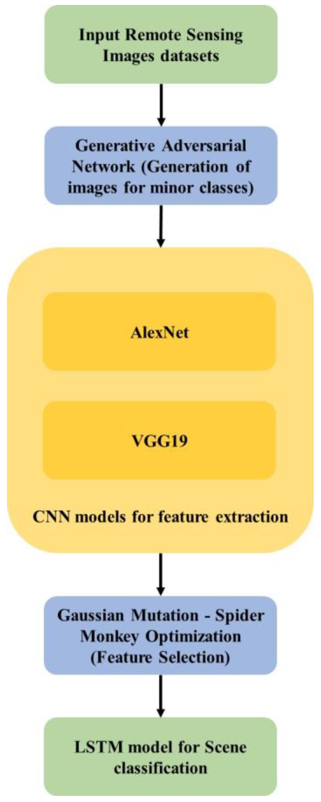
The GAN model is applied to three datasets such as UCM, AID, and NWPU45 to augment images in minority classes. The AlexNet and VGG19 models were applied to extract the features from input images. The GM-SMO model is applied to extracted features to select relevant features for classification. The overview of GM-SMO model in scene classification is shown in
Figure 1.
3.1. Dataset Description
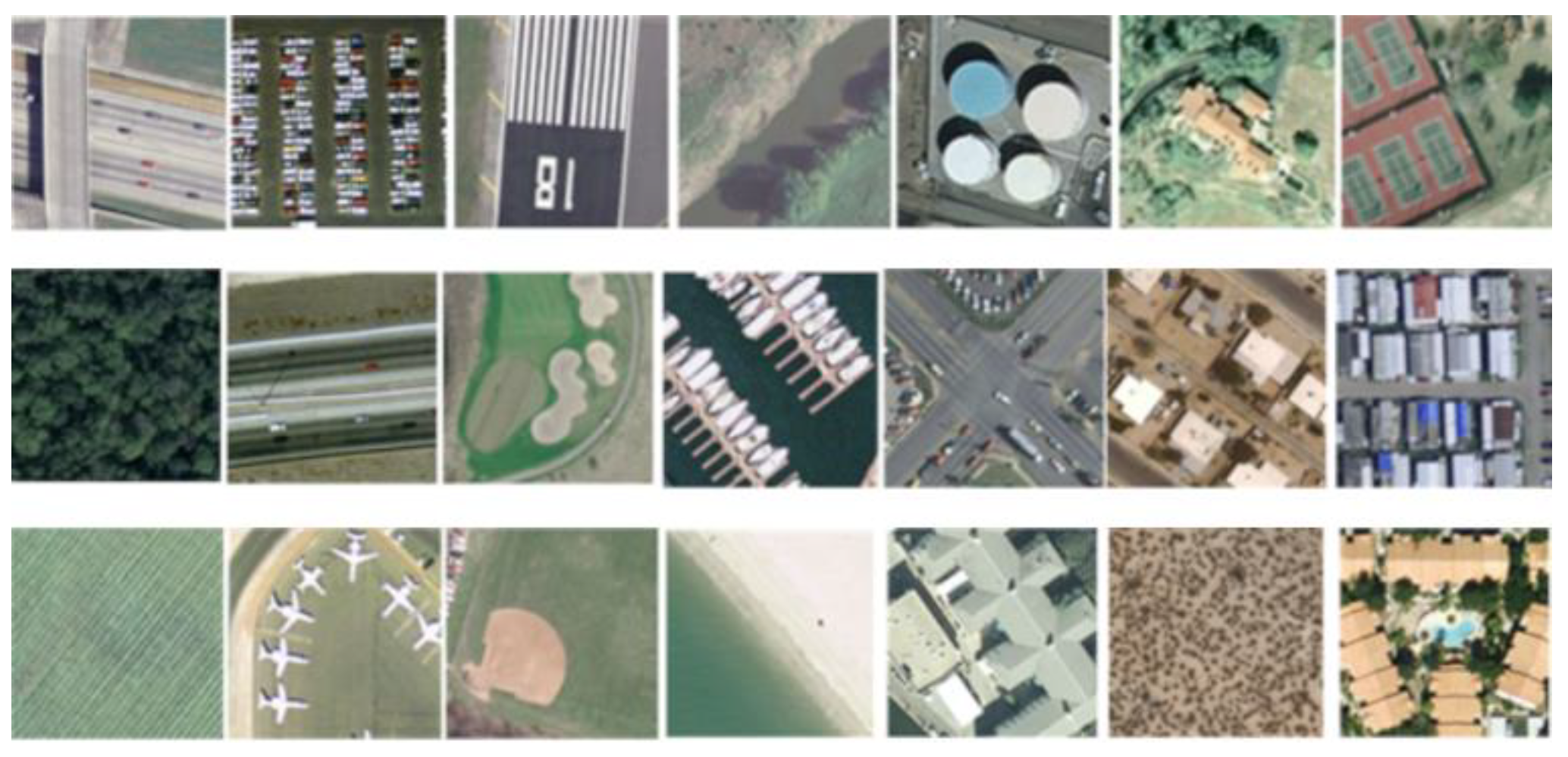
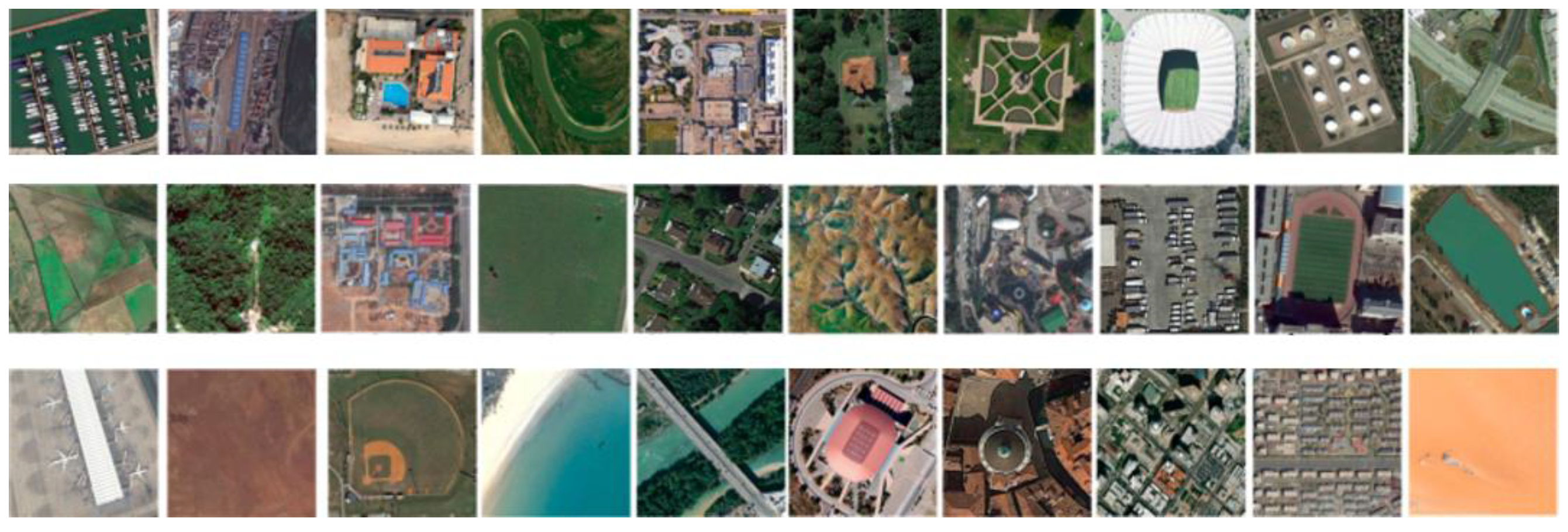
The proposed model’s performance is analyzed on three benchmark datasets such as UCM, AID, and NWPU45. The AID includes 10,000 images with pixel size of
and 0.5 to 8 m resolution, and it includes 30 classes. Correspondingly, the UCM dataset contains 2100 images with pixel size of
and resolution of 0.30 m, and it includes 21 classes. Additionally, the NWPU45 dataset comprises 31,500 images with pixel size of
and resolution of 0.2–30 m. The NWPU45 dataset covers more than 100 nations’ geo-locations and has 45 classes. The sample images of UCM, AID, and NWPU45 are represented in
Figure 2,
Figure 3 and
Figure 4.
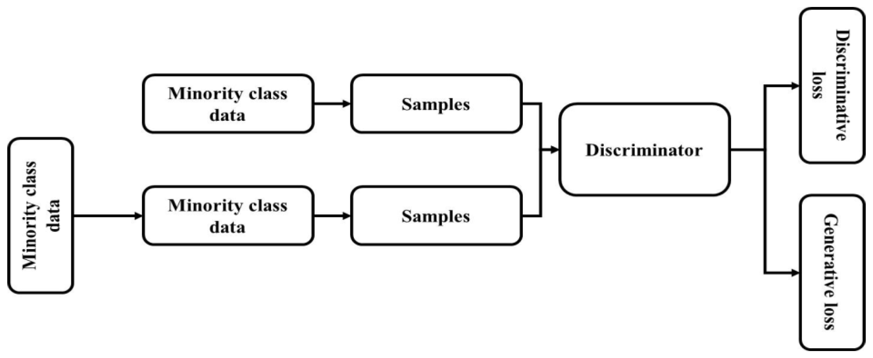
3.2. Generative Adversarial Network (GAN)
A generative model-specific framework is GANs. The generative model learns data distribution from samples set (images) to generate new images based on learned data distribution. GANs model and its variants are used for generating labeled images: one part of the model involves learning the objects in the images based on class, separately, and the other involves class related to labeled classes.
The first variant of GAN is Deep Convolutional GAN (DCGAN). Radford et al. [
31] proposed the architecture for both G and D networks of deep CNNs. This provides architectural steps for stable training of GAN and modification of Goodfellow et al. [
32] original GAN, which is the basics for recent GAN research. Two neural networks are present in a model that is used to train simultaneously. The discriminator is the first network and this is denoted as
. The discriminator’s role is to discriminate between samples real and fake. A sample
is imputed and output
is the probability of real samples. Generator
is second network and samples are generated in the generator and
D is real samples with high probability. The input samples
provide
from simple distribution
, usually a uniform distribution and the image space of distribution
maps
. The objective of the model is to
achieve
, as in Equation (1).
The is maximized to train the discriminator for images in the discriminator with and the model uses for images to minimize . The generates images in the generator to adjust during training such that . The generator is trained to increase , or equivalently reduce . The generator increases its ability to generate more realistic images during training and the discriminator increases its ability to differentiate the real from generated images.
Generator Architecture: The generator network considers a vector of 100 random numbers from uniform distribution as input and output are provided as objects in remote sensing images in the size of . The network architecture consists of a fully connected layer reshaped to a size of and an up-sample of four fractionally strided convolutions in kernel size of in the sample image. A deconvolution or fractionally-strided convolution is interpreted as pixels’ expansion by applying zeros in between them. A larger output image was generated by convolution of the expanded image. Each network layer is applied with batch-normalization excluding the output layer. In the GAN learning process, the entire mini-batch was stabilized using normalizing responses to have unit variance and zero mean and the generator was prevented from collapsing all samples. ReLU activation function was applied in all layers and the output layer was applied with tanh activation function.
Discriminator Architecture: A typical CNN architecture has a discriminator network that considers input images in the size of
and output is one decision (real or fake). The kernel size is set as
in four convolution layers of the network and a fully connected layer. Each convolution layer is applied with strided convolutions instead of pooling layers to reduce spatial dimensionality. Each layer of the network is applied with batch-normalization excluding input and output layers. Leaky ReLU activation functions
are applied in layers except for the output layer and sigmoid function with likelihood probability (0, 1) image score in the output layer. The Generative Adversarial Network’s [
33] architecture is shown in
Figure 5.
3.3. CNN-Based Feature Extraction
Convolution is a linear operation for feature extraction based on kernel, which is a small array of numbers. Kernel is applied on input for an array of numbers called a tensor [
34,
35].
A typical down-sampling operation is performed using a pooling layer to reduce feature maps of in-plane dimensionality. This introduces a translation invariance to small distortions and shifts, and decreases learnable parameters.
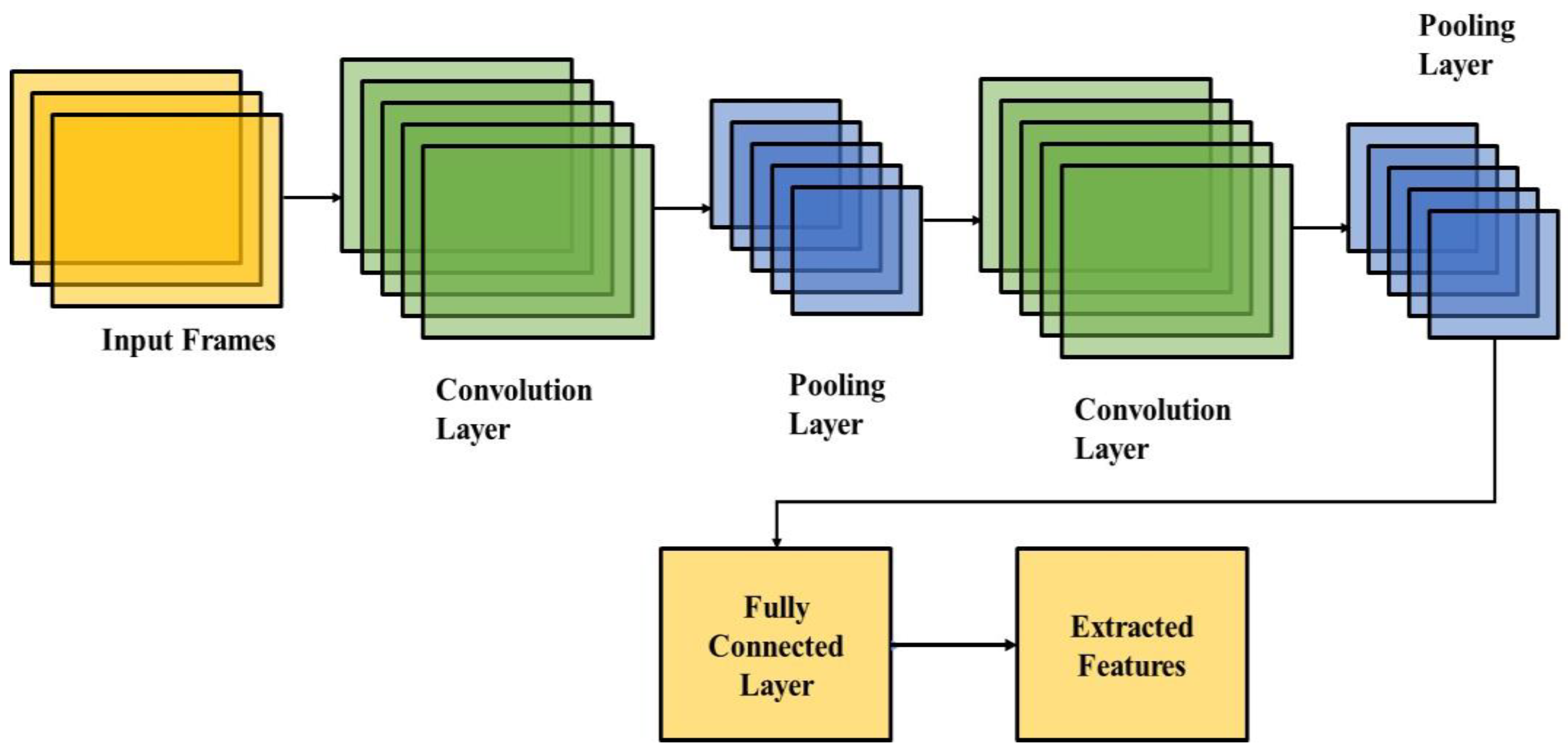
Pooling layer or final convolution of feature maps outputs are usually flattened, i.e., converted into a 1D array of numbers and connected to one or more fully connected layers, known as dense layers, so that every input is connected to a learnable weight of every output. The CNN architecture for feature extraction is shown in
Figure 6.
3.3.1. AlexNet
Various types of research [
36,
37] show AlexNet’s successful performance in classification and more significant performance in image processing than previous models. The researchers in deep learning show much interest in AlexNet due to its efficiency.
AlexNet model is applied with activation function and activation function provides neural networks’ non-linearity. Traditional activation functions are arctan function, tanh function, logistic function, etc. These functions generally cause gradient vanishing problems and a small range of 0 is applied with a larger gradient value. Rectified Linear Unit (ReLU) activation function is applied to overcome this problem. Equation (2) provides the ReLU model.
The ReLU gradient provides 1 output if the input is not less than 0. This shows that ReLU function provides higher convergence than tanh unit in deep networks. More acceleration is gained during the training process.
The dropout layer is applied in a fully connected layer to solve the overfitting problem. The dropout layer trains only a part of the neurons and skips the remaining neurons to avoid overfitting. For instance, if dropout is set as 0.1, then 10% of the neurons are skipped in training for every iteration. Generalization is improved by dropout to minimize neurons’ joint adaptation and cooperation between neurons. Dropout is applied on several sub-layers of the network. The same loss function is shared in each single sub-network and causes overfit to a certain extent. Sub-networks’ entire network output is provided and dropout improves the robustness of the model.
Convolution and pooling layers automatically perform feature extraction and reduction in the model. Convolutional layers are applied for images to increase the performance. Considering image
in
size and convolution are given in Equation (3).
where kernel
size is
, convolution provides a model solution to learn features of image and parameter sharing reduce complexity. Neighbouring pixel groups are applied in feature maps of pooling layer to reduce features and representation is provided by some values. The feature map size is
, and every 2 × 2 block has max value to generate max pooling and reduce for feature dimension.
Cross change normalization improves generalization. The same position of several adjacent maps sum is provided by cross channel normalization in neurons. Normalized feature maps are applied to next layers.
Fully connected layers perform classification and neurons are connected to adjacent neurons in next layer. These layers use softmax activation function for the classification.
Softmax output is present in the range of (0, 1) to activate neurons. Overlapping pooling is performed and various input images from datasets are used for AlexNet training. The AlexNet architecture for feature extraction is shown in
Figure 7.
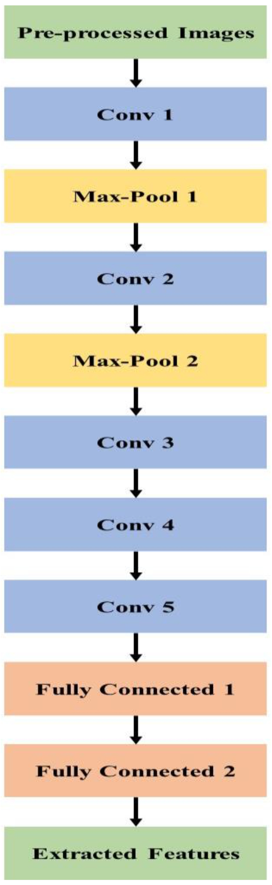
3.3.2. VGG 19
Oxford Robotics Institute developed a type of CNN model, which is named as Visual Geometry Group Network (VGG) [
38,
39]. VGGNet provides good performance in data cluster of ImageNet data. Five building blocks are present in VGG19. Two convolutional layers and one pooling layer are present in first and second building blocks, followed by four convolutional layers and one pooling layer which are present in the third and fourth blocks. Four convolutional layers are present in the final block and small filters
are used. The VGG19 architecture in feature extraction is shown in
Figure 8.
3.4. Spider Monkey Optimization
The SMO technique is a metaheuristic technique based on the social behavior of the spider monkey, adopting fusion and fission swarm intelligence for foraging [
40,
41,
42,
43]. Spider monkeys are in groups of 40 to 50 members. Food searching tasks in a territory are divided by a leader. Generally, spider monkeys live with 40 to 50 members of a swarm and a leader decides to partition food searching tasks in a territory. A female lead is selected as a global leader in the swarm and, in case of food insufficiency, this creates mutable smaller groups. The group size is based on food availability of specific territory. The spider monkey’s size is directly proportional to available food. The SMO based method of swarm intelligence (SI) satisfies the necessary conditions:
Labor division: smaller groups are created to divide foraging work for spider monkeys.
Self-organization: Food availability requirement is selected using group size.
An intelligent decision is carried out by intelligent foraging behavior.
Food search is initiated using swarm.
Food source individuals are measured using computing distance.
The food group members of individual’s distance alter the locations for the consideration.
Food source individual distance is calculated.
SMO method uses train and error for six phases of collaborative iterative process: global leader decision phase, learning phase, global leader, global leader phase, local leader decision phase, local leader learning phase, and local leader phase. The SMO method work flow is represented in
Figure 9.
The SMO method step-by-step process is given below.
3.4.1. Initializing
SMO method distributes population
of spider monkeys
(where
pth monkey of the population is denoted as
SMp, and
). Monkeys are
M-dimensional vectors, where total number of variables is denoted as
. One possible solution of each
is provided. SMO initializes each
using Equation (4).
where
is pth SM of qth dimension.
lower and upper bounds are and in the qth direction for random number of UR (0, 1), uniform distribution is in range of [0, 1].
3.4.2. Local Leader Phase (LLP)
The current location is changed by
SM using local group members and local leader past occurrences. The new location is updated for
SM location if fitness value of new location is higher than previous location. The location update of
pth
SM of
lth local group is provided in Equation (5):
where
The lth local group leader location of qth dimension is denoted as .
The lth local group of lth SM is randomly selected for qth dimension and is denoted as , such that .
3.4.3. Global Leader Phase (GLP)
After LLP, GLP is started to update the location. Experiences of local group members and global leader are used to update
SM location. The location update is provided in Equation (6):
where
qth dimension of global leader location is denoted as
and an arbitrarily selected index is
.
The
SM fitness calculates probability
in this phase. The location of
based on probability value, is updated and better location candidate has access to a number of possibilities to improve convergence. The probability calculation is given in Equation (7).
where
pth SM fitness value is denoted as
. The new location fitness of
SM’s is calculated and compared with the previous location. The best fitness value of the location is considered.
3.4.4. Global Leader Learning (GLL) Phase
The global leader location update is performed using a greedy selection technique. The SM location updated is based on the global leader location for best fitness in the population. The global leader is applied with the optimum location. An increment of 1 is added to Global Limit Count if updates are encountered.
3.4.5. Local Leader Learning (LLL) Phase
The local group is applied using the greedy selection method to update the location of the local leader. The SM location is updated with local leader location for best fitness in a specific local group. The local leader is assigned to the optimum location. The increment of 1 is added to the Local Limit Count if no updates are encountered.
3.4.6. Local Leader Decision (LLD) Phase
Local group candidates modify the location randomly as per step 1 when a local leader does not update its location or uses the past information from local and global leaders based on
using Equation (8).
3.4.7. Global Leader Decision (GLD) Phase
The population splits into small-size groups as per the global leader’s decision if the location is not updated for a global leader up to the Global Leader Limit. The splitting process occurs for a maximum number of groups (MG) is received. A local leader is selected at each iteration for the newly shaped group. Allowed groups are created at the maximum number and the global leader does not update its position until the allowed limit of pre-fixed, then global leader aims to merge entire groups into a single group.
The SMO processing controls parameters are as follows:
3.4.8. Gaussian Mutation
The SMO method is trapped in a local optimum in complex problems of the iterative optimization process. During iteration, the algorithm solution value remains unchanged. To increase the algorithm probability and algorithm shortcoming, this technique jumps out of the position of local optimal and adds random perturbation and Gaussian mutation and continues to process the algorithm. The Gaussian mutation formula is shown in Equation (9).
where random perturbation or Gaussian mutation selection probability is
and
was a random number in the range of [0, 1]. The distribution of Gaussian variation is given in Equation (10).
where the variance is denoted as
and the mean value is denoted as
.
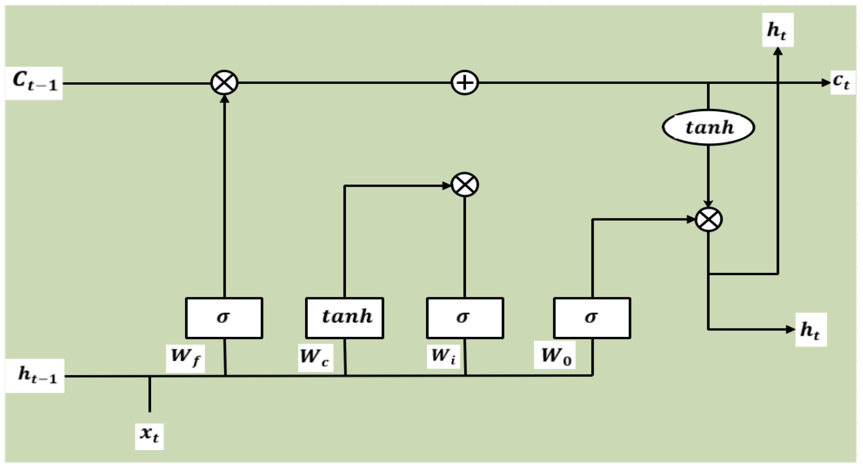
3.5. LSTM Model
The LSTM model is introduced by Hochreiter and Schmidhuber [
44] as an evolution of the RNN model. This model overcomes the limitation of RNN using additional interactions per module. LSTMs are a type of RNN that learn long-term dependencies and remember information for a long time as a default. A chain structure of the LSTM model is given in research [
45]. A different structure is present in the repeating module. Four interaction layers with unique communication method is applied instead of standard RNN or a single neural network. The LSTM structure is shown in
Figure 10.
A typical LSTM network consists of cells and memory blocks. The next cell is transferred into two states: a hidden state and a cell state. The main chain of data flow is the cell state that allows data to flow essentially unchained. Some linear transformation is carried out and sigmoid is used to remove or add data in the layer. A gate is similar to a series of matrix operations or a layer that has various individual weights. LSTMs are developed to reduce long-term dependency using memorizing process to control gates [
46].
4. Experimental Setup
The implementation details of datasets, parameter settings, and system requirements are discussed in this section.
Datasets: The UCM [
47] dataset has 100 images per class, 21 classes, 2100 total images, 0.3 m spatial resolution, and
image size. The AID [
48] dataset has 200–400 images per class, 30 classes, 10,000 total images, 0.5–0.8 m spatial resolution, and
image size. The NWPU45 [
49] dataset has 700 images per class, 40 classes, 31,500 total images, 0.2–0.3 m spatial resolution, and
image size. As seen in the AID, the number of images varied per class, where this imbalanced data problem is effectively addressed by the GM-SMO model.
Parameter settings: In AlexNet and VGG19 model, the learning rate is set as 0.01, the dropout rate is set as 0.1, and the Adam optimizer is used. In LSTM network, the loss function is categorical cross entropy loss function and optimizer is Adam. In GM-SMO, the population size is set as 50, and number of iterations is set as 50. The 5-fold cross validation is applied to test the performance of the model.
System Requirement: Intel i9 processor, RAM is 128 GB, Graphics card is 22 GB, and OS is Windows 10-64 bit. MATLAB 2022a was used to evaluate the performance of the GM-SMO technique.
5. Results
The GM-SMO model is applied to scene classification to improve the efficiency of the model. The GM-SMO model is tested on three datasets and accuracy is shown for 10 epochs. The GM-SMO model is tested and compared with deep learning techniques and feature selection techniques on scene classification. The GM-SMO model is also compared with existing methods in scene classification for three datasets. The Grey Wolf Optimization (GWO), Firefly (FF), and Particle Swarm Optimization (PSO) were compared with the GM-SMO technique on scene classification.
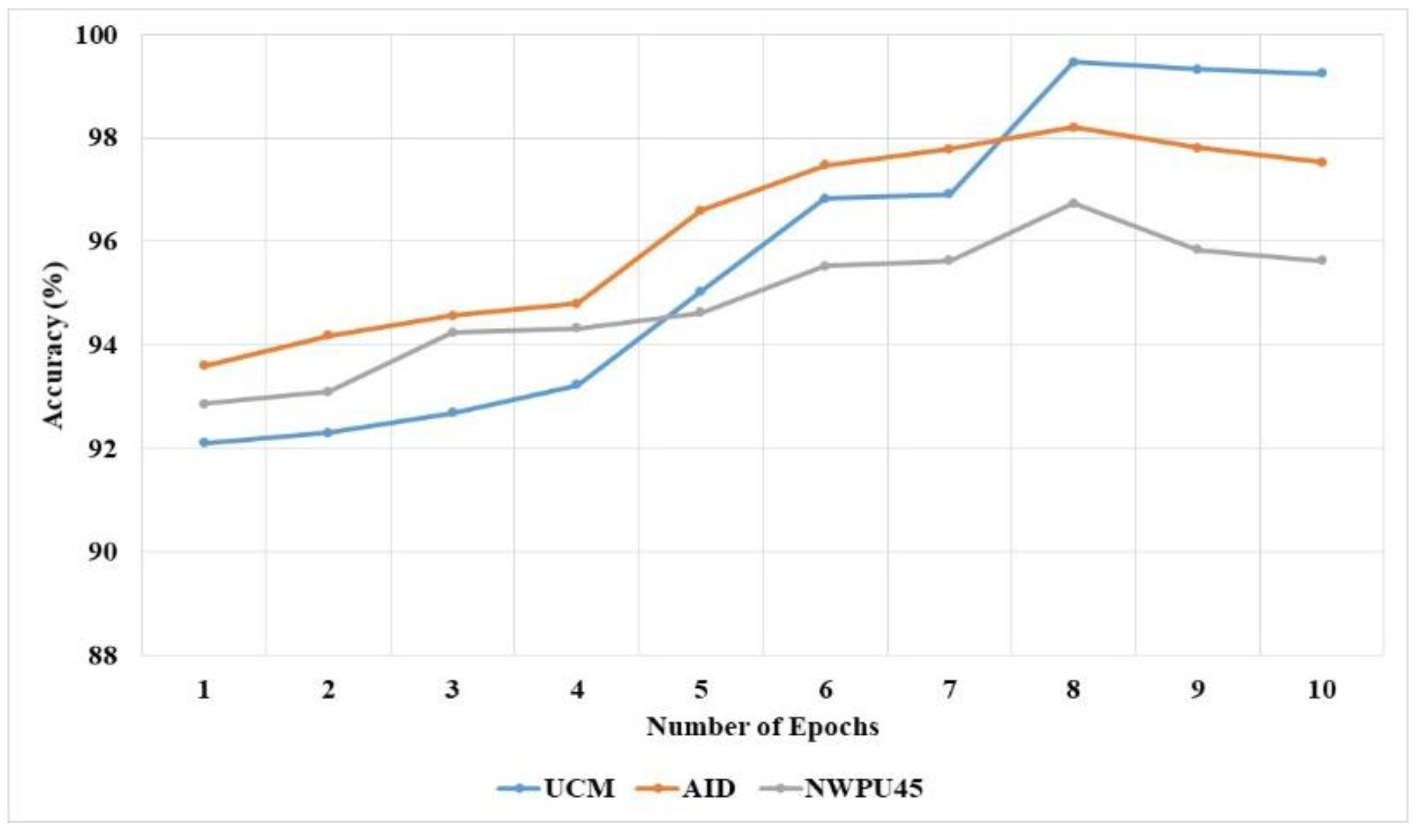
The GM-SMO method accuracy for various numbers of epochs for three datasets is shown in
Figure 11. This shows that the GM-SMO method increases the accuracy up to 8 epochs and accuracy decreases after 8 epochs. The reason for the decrease in accuracy after 8 epochs is the overfitting problem. The generation of more features in the convolutional layer and repeated learning of the features creates an overfitting problem. The Gaussian mutation in the SMO method helps to learn unique features for classification and increases the exploitation. The Gaussian mutation technique helps to reduce the overfitting problem and increases the performance of classification.
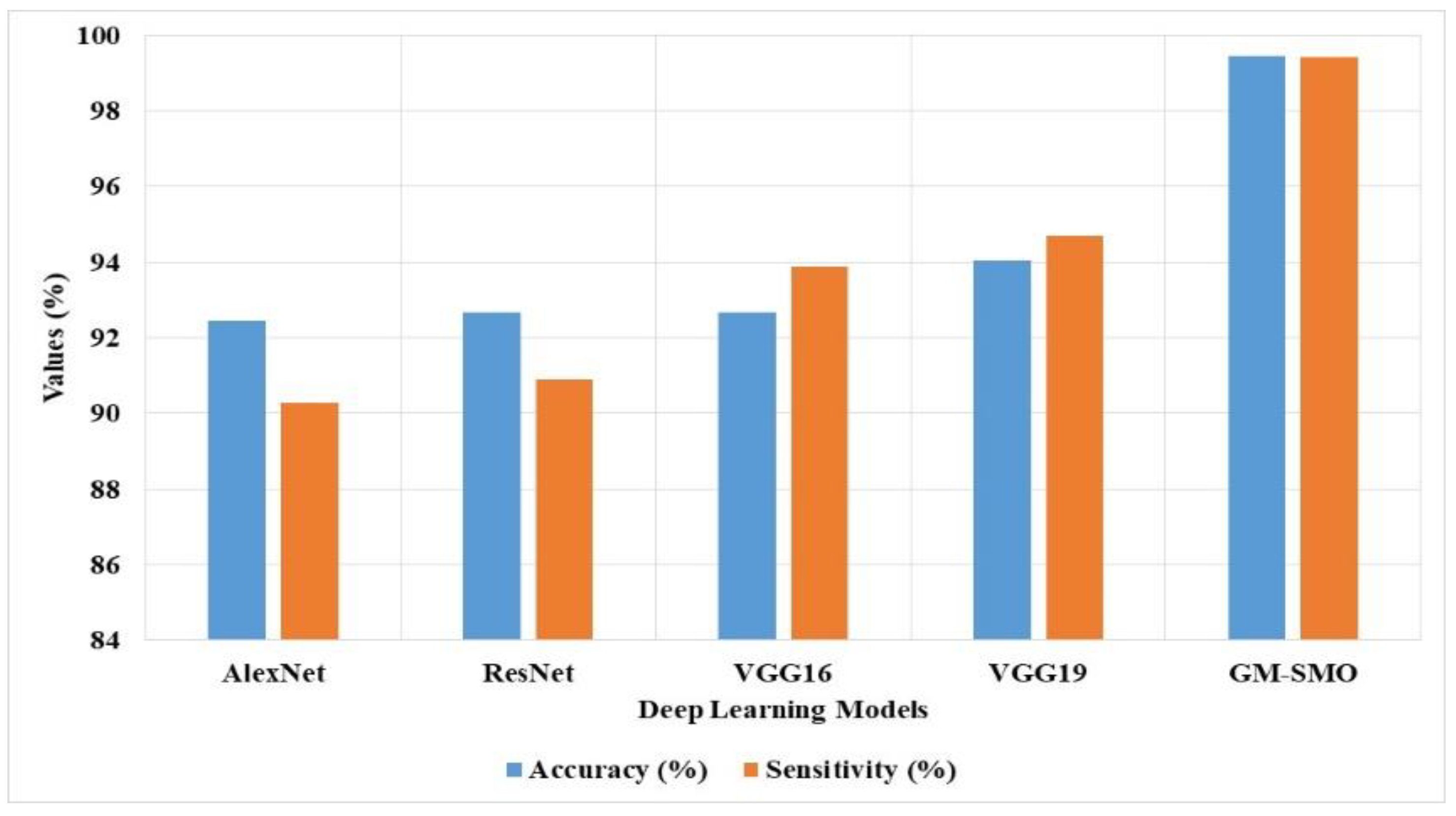
The GM-SMO method is measured with accuracy and sensitivity for three datasets and compared with deep learning techniques, as shown in
Table 1 and
Figure 12. The GM-SMO model uses the AlexNet-VGG19 model for feature extraction from given images. The GM-SMO method performs feature selection with better exploitation that helps to reduce the overfitting problem in scene classification. The existing deep learning models such as GoogleNet, ResNet, Artificial Neural Network (ANN), and Recurrent Neural Network (RNN) have overfitting problems and provide lower efficiency. The existing method generates more features in the convolutional layer and lacks feature selection techniques for classification. The GM-SMO with LSTM has obtained higher performance than the existing techniques in scene classification. The GM-SMO with LSTM has 99.46% accuracy and 99.41% sensitivity, which are better than the other models. The local understanding of the images is good enough in the GM-SMO with LSTM model; therefore, it obtains better classification results compared to other classification models. In addition, the Z-test’s
p-value of individual classifiers is mentioned in
Table 1.
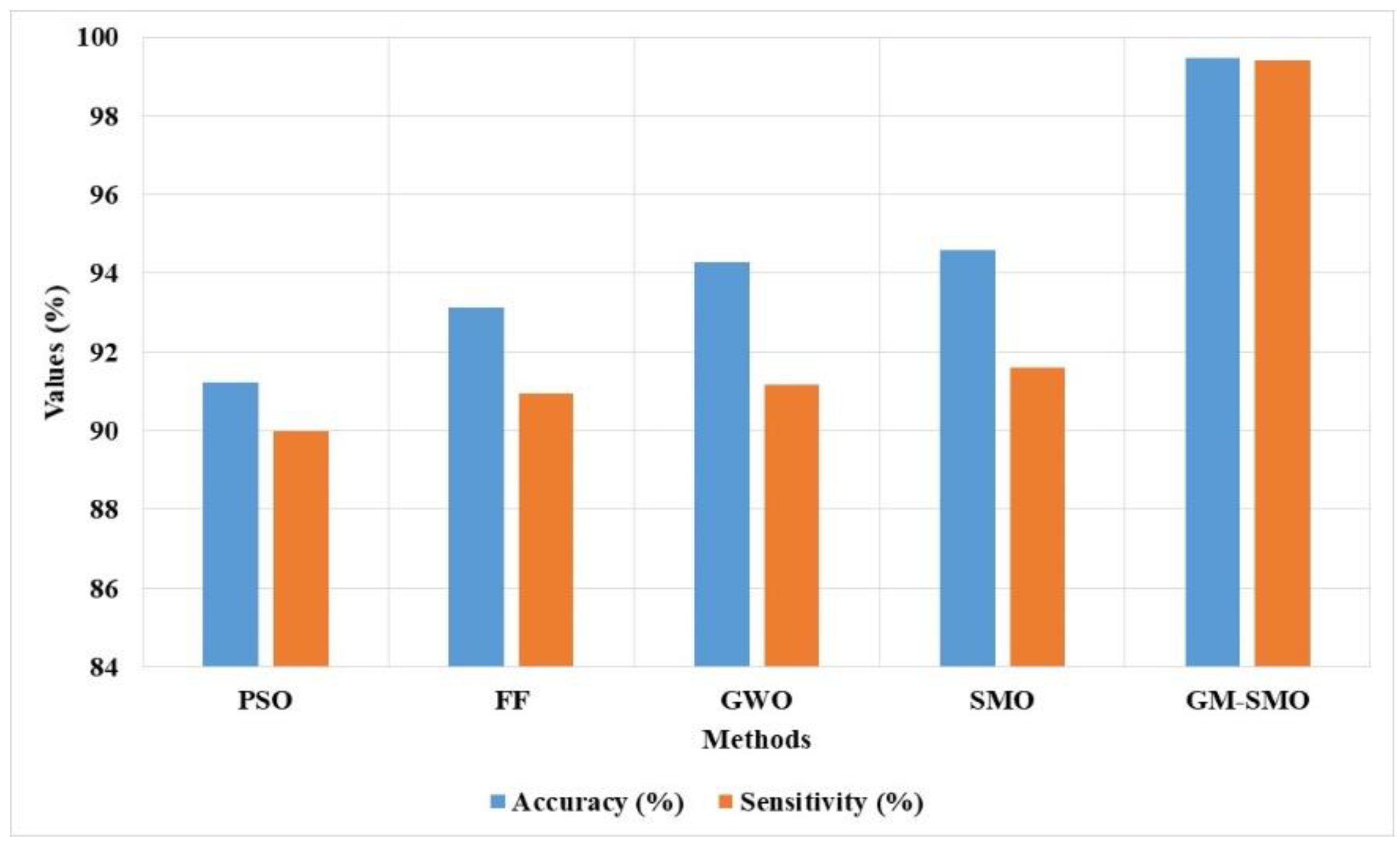
The GM-SMO method performance is compared with existing feature selection techniques, as shown in
Table 2 and
Figure 13. The existing feature selection techniques such as GWO, FF, and PSO have a limitation of local optima trap due to lower exploitation. The Gaussian mutation is applied in the SMO technique to increase the exploitation and overcome the overfitting problem. The Gaussian mutation changes the solutions related to the best solution that increases the exploitation in feature selection. The GM-SMO model selects unique features for scene classification that help to increase the sensitivity of the model. The GM-SMO model has 99.46% accuracy and 99.41% sensitivity, which are better compared to the existing optimizers.
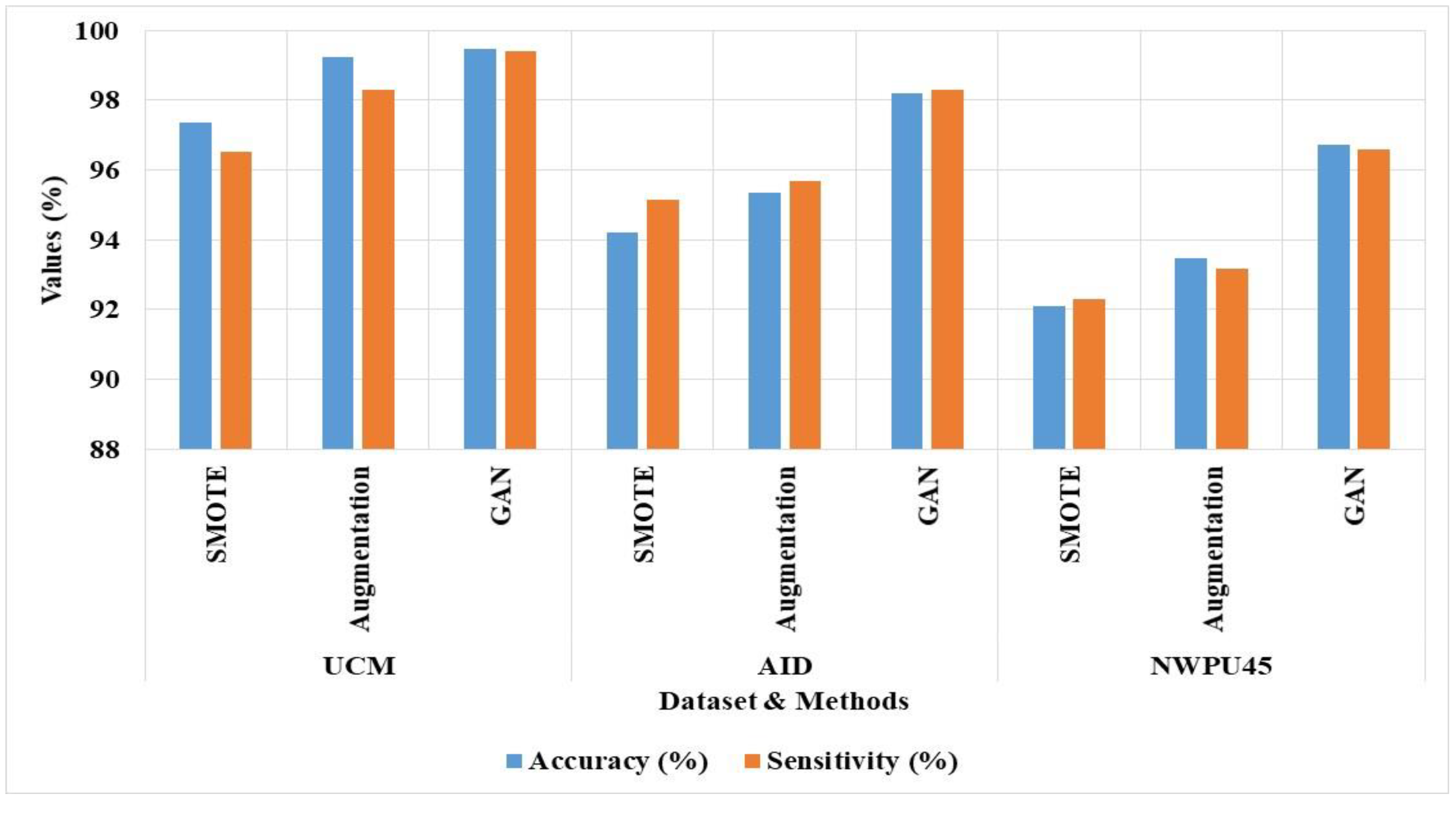
The imbalanced data problem decreases the performance of scene classification in existing techniques. A common technique applied for imbalanced data problems is augmentation to generate similar images.
Table 3 and
Figure 14 show the GAN augmentation performance with standard augmentation. Although images generated by augmentation are highly similar, it is difficult to learn unique features, overfitting, and misclassification among similar categories. GAN based augmentation is applied in this study to generate similar images in minority classes and unique feature learning. The GAN based optimization technique has higher efficiency in three datasets than augmentation and SMOTE techniques. The GAM GM-SMO method has 99.46% accuracy and 99.41% sensitivity, and augmentation model has 99.24% accuracy and 98.31% sensitivity in UCM dataset.
By inspecting
Table 4, the proposed GM-SMO with LSTM classifier obtained higher classification results compared to other classifiers: GoogleNet, ResNet, ANN, and RNN, with limited computational time. As specified in
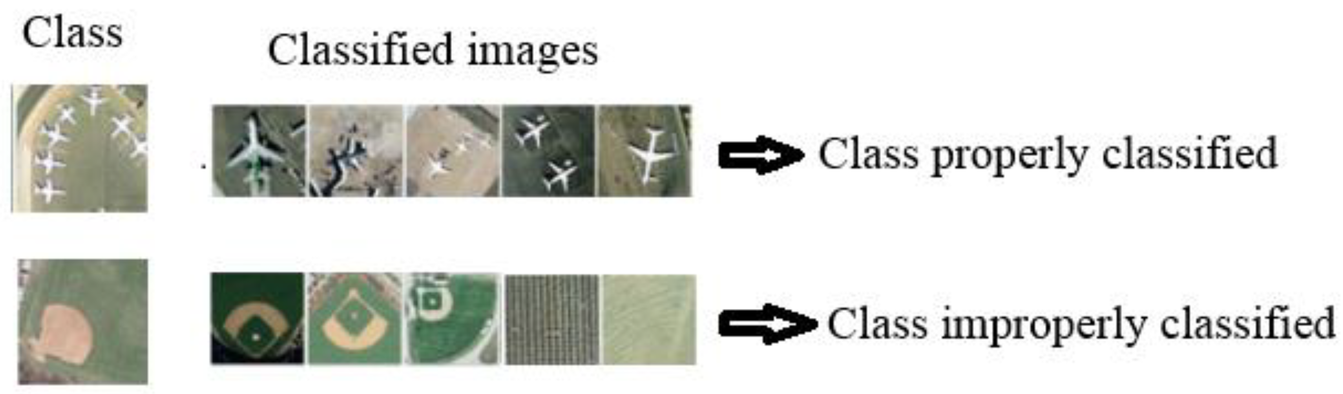
Table 4, the GM-SMO with LSTM classifier consumed 12, 23, and 34 s per image of computation time on the UCM, AID, and NWPU45 datasets. Sample classification output image is depicted in
Figure 15.
Comparative Analysis
The GM-SMO model is compared with existing techniques in scene classification on three datasets such as UCM, AID, and NWPU45, and the comparative results are mentioned in
Table 5,
Table 6 and
Table 7. The GM-SMO method is compared with existing techniques on the UCM dataset, as shown in
Table 5. The existing CNN model has limitations of imbalanced data problem and overfitting problem in the scene classification. The GM-SMO model applies the GAN model to augment the minority classes and increase their performance. The Gaussian mutation changes the solution after exploration to increase the exploitation of the model. The GM-SMO method selects the unique features to overcome the overfitting and imbalanced data problem. The GM-SMO model has achieved 99.46% accuracy, which is better compared to other methods on the UCM dataset.
The GM-SMO model is compared with existing techniques in scene classification on the AID dataset, as shown in
Table 6. The GM-SMO model selects unique features for the classification to solve the overfitting problem and imbalanced data problem. The GM-SMO model changes the solution of the SMO technique to increase the exploitation of the model. The GM-SMO model has achieved 98.20% accuracy, which is superior compared to other models on the AID dataset.
The GM-SMO method is compared with existing scene classification techniques on NWPU45 dataset, as shown in
Table 7. The existing CNN based models have a limitation of imbalanced data problem and overfitting problem in scene classification. The GM-SMO model changes the solution of SMO technique after exploration to increase the exploitation. The GM-SMO model maintains the tradeoff between exploration and exploitation to find the relevant features for classification. The GM-SMO model selects unique features to overcome the overfitting and imbalanced data problem. The GM-SMO model has 96.73% accuracy, which is better compared to transformers—CNN [
30], MA-GRN [
29], and other comparative models.
6. Conclusions
Scene classification helps to classify the object or land use such as a farm, airplane, or stadium from remote sensing images. The existing CNN based models have limitations of overfitting problems, imbalanced data problems, and misclassification of similar categories. This research proposes a GM-SMO technique for the feature selection process to improve the classification performance of scene classification. The GM-SMO model selects unique features to overcome the imbalanced data problem and overfitting problem. The GAN model is applied for the augmentation of images and to reduce imbalanced data problems. The AlexNet and VGG19 models are applied to extract the features from remote sensing images. The GM-SMO model has 98.20% accuracy, LSE-Net has 94.41% accuracy, and MTLN has 92.54% accuracy on the AID dataset. The future work of this research involves applying the proposed model to the real time datasets to further validate the efficiency of the model. However, the proposed model is computationally complex, which can be addressed in future work by implementing an unsupervised deep learning model.
Author Contributions
The paper investigation, resources, data curation, writing—original draft preparation, writing—review and editing, and visualization were conducted by A.L.H.P.S. and M.K.M. The paper conceptualization and software were conducted by R.R.A. and A.K.P. The validation, formal analysis, methodology, supervision, project administration, and funding acquisition of the version to be published were conducted by C.-M.C. All authors have read and agreed to the published version of the manuscript.
Funding
This research is supported by Shandong Provincial Natural Science Foundation with project number : ZR202111290043.
Data Availability Statement
Conflicts of Interest
The authors declare no conflict of interest.
References
- Xie, H.; Chen, Y.; Ghamisi, P. Remote sensing image scene classification via label augmentation and intra-class constraint. Remote Sens. 2021, 13, 2566. [Google Scholar] [CrossRef]
- Li, Y.; Zhu, Z.; Yu, J.G.; Zhang, Y. Learning deep cross-modal embedding networks for zero-shot remote sensing image scene classification. IEEE Trans. Geosci. Remote Sens. 2021, 59, 10590–10603. [Google Scholar] [CrossRef]
- Li, M.; Lin, L.; Tang, Y.; Sun, Y.; Kuang. G. An attention-guided multilayer feature aggregation network for remote sensing image scene classification. Remote Sens. 2021, 13, 3113. [Google Scholar] [CrossRef]
- Wang, X.; Wang, S.; Ning, C.; Zhou, H. Enhanced feature pyramid network with deep semantic embedding for remote sensing scene classification. IEEE Trans. Geosci. Remote Sens. 2021, 59, 7918–7932. [Google Scholar] [CrossRef]
- Cheng, G.; Sun, X.; Li, K.; Guo, L.; Han, J. Perturbation-seeking generative adversarial networks: A defense framework for remote sensing image scene classification. IEEE Trans. Geosci. Remote Sens. 2021, 60, 5605111. [Google Scholar] [CrossRef]
- Srinivas, M.; Roy, D.; Mohan, C.K. Discriminative feature extraction from X-ray images using deep convolutional neural networks. In Proceedings of the 2016 IEEE International Conference on Acoustics, Speech and Signal Processing (ICASSP), Shanghai, China, 20–25 March 2016; pp. 917–921. [Google Scholar]
- Ijjina, E.P.; Mohan, C.K. Human action recognition based on recognition of linear patterns in action bank features using convolutional neural networks. In Proceedings of the 2014 13th International Conference on Machine Learning and Applications, Detroit, MI, USA, 3–6 December 2014; pp. 178–182. [Google Scholar]
- Saini, R.; Jha, N.K.; Das, B.; Mittal, S.; Mohan, C.K. Ulsam: Ultra-lightweight subspace attention module for compact convolutional neural networks. In Proceedings of the IEEE/CVF Winter Conference on Applications of Computer Vision, Snowmass, CO, USA, 1–5 March 2020; pp. 1627–1636. [Google Scholar]
- Deepak, K.; Chandrakala, S.; Mohan, C.K. Residual spatiotemporal autoencoder for unsupervised video anomaly detection. Signal Image Video Process 2021, 15, 215–222. [Google Scholar] [CrossRef]
- Roy, D.; Murty, K.S.R.; Mohan, C.K. Unsupervised universal attribute modeling for action recognition. IEEE Trans. Multimed. 2018, 21, 1672–1680. [Google Scholar] [CrossRef]
- Perveen, N.; Roy, D.; Mohan, C.K. Spontaneous expression recognition using universal attribute model. IEEE Trans. Image Process 2018, 27, 5575–5584. [Google Scholar] [CrossRef]
- Roy, D.; Ishizaka, T.; Mohan, C.K.; Fukuda, A. Vehicle trajectory prediction at intersections using interaction based generative adversarial networks. In Proceedings of the 2019 IEEE Intelligent Transportation Systems Conference (ITSC), Auckland, New Zealand, 27–30 October 2019; pp. 2318–2323. [Google Scholar]
- Roy, D. Snatch theft detection in unconstrained surveillance videos using action attribute modelling. Pattern Recognit. Lett. 2018, 108, 56–61. [Google Scholar] [CrossRef]
- Zhang, P.; Bai, Y.; Wang, D.; Bai, B.; Li, Y. Few-shot classification of aerial scene images via meta-learning. Remote Sens. 2021, 13, 108. [Google Scholar] [CrossRef]
- Kim, J.; Chi, M. SAFFNet: Self-attention-based feature fusion network for remote sensing few-shot scene classification. Remote Sens. 2021, 13, 2532. [Google Scholar] [CrossRef]
- Zhang, Z.; Liu, S.; Zhang, Y.; Chen, W. RS-DARTS: A convolutional neural architecture search for remote sensing image scene classification. Remote Sens. 2021, 14, 141. [Google Scholar] [CrossRef]
- Wu, X.; Zhang, Z.; Zhang, W.; Yi, Y.; Zhang, C.; Xu, Q. A convolutional neural network based on grouping structure for scene classification. Remote Sens. 2021, 13, 2457. [Google Scholar] [CrossRef]
- Lasloum, T.; Alhichri, H.; Bazi, Y.; Alajlan, N. SSDAN: Multi-source semi-supervised domain adaptation network for remote sensing scene classification. Remote Sens. 2021, 13, 3861. [Google Scholar] [CrossRef]
- Xu, K.; Huang, H.; Deng, P.; Li, Y. Deep feature aggregation framework driven by graph convolutional network for scene classification in remote sensing. IEEE Trans. Neural Netw. Learn. Syst. 2021, 33, 5751–5765. [Google Scholar] [CrossRef]
- Bazi, Y.; Bashmal, L.; Rahhal, M.M.A.; Dayil, R.A.; Ajlan, N.A. Vision transformers for remote sensing image classification. Remote Sens. 2021, 13, 516. [Google Scholar] [CrossRef]
- Alhichri, H.; Alswayed, A.S.; Bazi, Y.; Ammour, N.; Alajlan, N.A. Classification of remote sensing images using EfficientNet-B3 CNN model with attention. IEEE Access 2021, 9, 14078–14094. [Google Scholar] [CrossRef]
- Ma, A.; Wan, Y.; Zhong, Y.; Wang, J.; Zhang, L. SceneNet: Remote sensing scene classification deep learning network using multi-objective neural evolution architecture search. ISPRS J. Photogramm. Remote Sens. 2021, 172, 171–188. [Google Scholar] [CrossRef]
- Zheng, X.; Gong, T.; Li, X.; Lu, X. Generalized scene classification from small-scale datasets with multitask learning. IEEE Trans. Geosci. Remote Sens. 2021, 60, 5609311. [Google Scholar] [CrossRef]
- Xu, K.; Huang, H.; Deng, P. Remote sensing image scene classification based on global–local dual-branch structure model. IEEE Geosci. Remote Sens. Lett. 2021, 19, 8011605. [Google Scholar] [CrossRef]
- Tang, X.; Ma, Q.; Zhang, X.; Liu, F.; Ma, J.; Jiao, L. Attention consistent network for remote sensing scene classification. IEEE J. Sel. Top. Appl. Earth Obs. Remote Sens. 2021, 14, 2030–2045. [Google Scholar] [CrossRef]
- Bi, Q.; Qin, K.; Zhang, H.; Xia, G.S. Local semantic enhanced convnet for aerial scene recognition. IEEE Trans. Image Process 2021, 30, 6498–6511. [Google Scholar] [CrossRef] [PubMed]
- Cheng, G.; Cai, L.; Lang, C.; Yao, X.; Chen, J.; Guo, L.; Han, J. SPNet: Siamese-prototype network for few-shot remote sensing image scene classification. IEEE Trans. Geosci. Remote Sens. 2021, 60, 5608011. [Google Scholar] [CrossRef]
- Zareapoor, M.; Chanussot, J.; Zhou, H.; Yang, J. Rotation Equivariant Feature Image Pyramid Network for Object Detection in Optical Remote Sensing Imagery. IEEE Trans. Geosci. Remote Sens. 2021, 60, 5608614. [Google Scholar]
- Li, B.; Guo, Y.; Yang, J.; Wang, L.; Wang, Y.; An, W. Gated recurrent multiattention network for VHR remote sensing image classification. IEEE Trans. Geosci. Remote Sens. 2021, 60, 5606113. [Google Scholar] [CrossRef]
- Zhang, J.; Zhao, H.; Li, J. TRS: Transformers for remote sensing scene classification. Remote Sens. 2021, 13, 4143. [Google Scholar] [CrossRef]
- Radford, A.; Metz, L.; Chintala, S. Unsupervised representation learning with deep convolutional generative adversarial networks. arXiv 2015, arXiv:1511.06434. [Google Scholar]
- Goodfellow, I.; Pouget-Abadie, J.; Mirza, M.; Xu, B.; Warde-Farley, D.; Ozair, S.; Courville, A.; Bengio, Y. Generative adversarial nets. In Proceedings of the 28th Annual Conference on Neural Information Processing Systems 2014 (NIPS), Montreal, QC, Canada, 8–13 December 2014; p. 27. [Google Scholar]
- Yi, X.; Walia, E.; Babyn, P. Generative adversarial network in medical imaging: A review. Med. Image Anal. 2019, 58, 101552. [Google Scholar] [CrossRef] [Green Version]
- Niu, M.; Lin, Y.; Zou, Q. sgRNACNN: Identifying sgRNA on-target activity in four crops using ensembles of convolutional neural networks. Plant Mol. Biol. 2021, 105, 483–495. [Google Scholar] [CrossRef]
- Zhang, Z.; Tian, J.; Huang, W.; Yin, L.; Zheng, W.; Liu, S. A haze prediction method based on one-dimensional convolutional neural network. Atmosphere 2021, 12, 1327. [Google Scholar] [CrossRef]
- Chen, J.; Wan, Z.; Zhang, J.; Li, W.; Chen, Y.; Li, Y.; Duan, Y. Medical image segmentation and reconstruction of prostate tumor based on 3D AlexNet. Comput. Methods Programs Biomed. 2021, 200, 105878. [Google Scholar] [CrossRef] [PubMed]
- Zhu, Y.; Li, G.; Wang, R.; Tang, S.; Su, H.; Cao, K. Intelligent fault diagnosis of hydraulic piston pump based on wavelet analysis and improved alexnet. Sensors 2021, 21, 549. [Google Scholar] [CrossRef] [PubMed]
- Karacı, A. VGGCOV19-NET: Automatic detection of COVID-19 cases from X-ray images using modified VGG19 CNN architecture and YOLO algorithm. Neural Comput. Appl. 2022, 34, 8253–8274. [Google Scholar] [CrossRef] [PubMed]
- Awan, M.J.; Masood, O.A.; Mohammed, M.A.; Yasin, A.; Zain, A.M.; Damaševičius, R.; Abdulkareem, K.H. Image-Based Malware Classification Using VGG19 Network and Spatial Convolutional Attention. Electronics 2021, 10, 2444. [Google Scholar] [CrossRef]
- Kumar, S.; Sharma, B.; Sharma, V.K.; Sharma, H.; Bansal, J.C. Plant leaf disease identification using exponential spider monkey optimization. Sustain. Comput. Inform. Syst. 2020, 28, 100283. [Google Scholar] [CrossRef]
- Kumar, S.; Sharma, B.; Sharma, V.K.; Poonia, R.C. Automated soil prediction using bag-of-features and chaotic spider monkey optimization algorithm. Evol. Intell. 2021, 14, 293–304. [Google Scholar] [CrossRef]
- Lee, J.G.; Chim, S.; Park, H.H. Energy-efficient cluster-head selection for wireless sensor networks using sampling-based spider monkey optimization. Sensors 2019, 19, 5281. [Google Scholar] [CrossRef] [Green Version]
- Xia, X.; Liao, W.; Zhang, Y.; Peng, X. A discrete spider monkey optimization for the vehicle routing problem with stochastic demands. Appl. Soft Comput. 2021, 111, 107676. [Google Scholar] [CrossRef]
- Jalayer, M.; Orsenigo, C.; Vercellis, C. Fault detection and diagnosis for rotating machinery: A model based on convolutional LSTM, Fast Fourier and continuous wavelet transforms. Comput. Ind. 2021, 125, 103378. [Google Scholar] [CrossRef]
- Yang, Y.; Xiong, Q.; Wu, C.; Zou, Q.; Yu, Y.; Yi, H.; Gao, M. A study on water quality prediction by a hybrid CNN-LSTM model with attention mechanism. Environ. Sci. Pollut. Res. 2021, 28, 55129–55139. [Google Scholar] [CrossRef]
- Kumar, S.; Damaraju, A.; Kumar, A.; Kumari, S.; Chen, C.-M. LSTM network for transportation mode detection. J. Internet Technol. 2021, 22, 891–902. [Google Scholar] [CrossRef]
- Yang, Y.; Newsam, S. Bag-of-visual-words and spatial extensions for land-use classification. In Proceedings of the 18th SIGSPATIAL International Conference on Advances in Geographic Information Systems, San Jose, CA, USA, 2–5 November 2010; pp. 270–279. [Google Scholar]
- Xia, G.S.; Hu, J.; Hu, F.; Shi, B.; Bai, X.; Zhong, Y.; Zhang, L.; Lu, X. AID: A benchmark data set for performance evaluation of aerial scene classification. IEEE Trans. Geosci. Remote Sens. 2017, 55, 3965–3981. [Google Scholar] [CrossRef]
- Li, B.; Su, W.; Wu, H.; Li, R.; Zhang, W.; Qin, W.; Zhang, S. Aggregated deep fisher feature for VHR remote sensing scene classification. IEEE J. Sel. Top. Appl. Earth Obs. Remote Sens. 2019, 12, 3508–3523. [Google Scholar] [CrossRef]
Figure 1.
GM-SMO feature selection and CNN based feature extraction model for remote sensing scene classification.
Figure 1.
GM-SMO feature selection and CNN based feature extraction model for remote sensing scene classification.
Figure 2.
Sample images of UCM dataset.
Figure 2.
Sample images of UCM dataset.
Figure 3.
Sample images of AID dataset.
Figure 3.
Sample images of AID dataset.
Figure 4.
Sample images of NWPU45 dataset.
Figure 4.
Sample images of NWPU45 dataset.
Figure 5.
Generative Adversarial Network for generation of images in minority classes.
Figure 5.
Generative Adversarial Network for generation of images in minority classes.
Figure 6.
Convolutional Neural Network architecture for feature extraction process.
Figure 6.
Convolutional Neural Network architecture for feature extraction process.
Figure 7.
AlexNet model for feature extraction scene classification.
Figure 7.
AlexNet model for feature extraction scene classification.
Figure 8.
VGG19 architecture for feature extraction on scene classification.
Figure 8.
VGG19 architecture for feature extraction on scene classification.
Figure 9.
Gaussian Mutation–Spider Monkey Optimization for feature selection on scene classification.
Figure 9.
Gaussian Mutation–Spider Monkey Optimization for feature selection on scene classification.
Figure 10.
LSTM unit for remote sensing scene classification.
Figure 10.
LSTM unit for remote sensing scene classification.
Figure 11.
GM-SMO method accuracy vs. number of epochs in scene classification.
Figure 11.
GM-SMO method accuracy vs. number of epochs in scene classification.
Figure 12.
GM-SMO method’s accuracy and sensitivity compared with deep learning in three datasets.
Figure 12.
GM-SMO method’s accuracy and sensitivity compared with deep learning in three datasets.
Figure 13.
GM-SMO method accuracy and sensitivity compared with existing feature selection techniques.
Figure 13.
GM-SMO method accuracy and sensitivity compared with existing feature selection techniques.
Figure 14.
GM-SMO performance in the sampling process.
Figure 14.
GM-SMO performance in the sampling process.
Figure 15.
Sample classification output image.
Figure 15.
Sample classification output image.
Table 1.
Deep learning techniques’ performance in scene classification on three datasets.
Table 1.
Deep learning techniques’ performance in scene classification on three datasets.
| Methods | Accuracy (%) | Sensitivity (%) | p-Value |
|---|
| GoogleNet | 92.44 | 90.28 | <0.10 |
| ResNet | 92.67 | 90.9 | <0.10 |
| ANN | 92.67 | 93.89 | <0.05 |
| RNN | 94.04 | 94.68 | <0.05 |
| LSTM with GM-SMO | 99.46 | 99.41 | <0.01 |
Table 2.
Feature selection techniques’ comparison in scene classification on three datasets.
Table 2.
Feature selection techniques’ comparison in scene classification on three datasets.
| Methods | Accuracy (%) | Sensitivity (%) |
|---|
| PSO | 91.23 | 90 |
| FF | 93.14 | 90.94 |
| GWO | 94.28 | 91.18 |
| SMO | 94.6 | 91.6 |
| GM-SMO | 99.46 | 99.41 |
Table 3.
Sampling techniques for scene classification.
Table 3.
Sampling techniques for scene classification.
| Datasets | Methods | Accuracy (%) | Sensitivity (%) |
|---|
| UCM | SMOTE | 97.35 | 96.53 |
| Augmentation | 99.24 | 98.31 |
| GAN | 99.46 | 99.41 |
| AID | SMOTE | 94.2 | 95.14 |
| Augmentation | 95.34 | 95.67 |
| GAN | 98.2 | 98.31 |
| NWPU45 | SMOTE | 92.1 | 92.3 |
| Augmentation | 93.46 | 93.16 |
| GAN | 96.73 | 96.6 |
Table 4.
Results of the GM-SMO with LSTM classifier in terms of means of computational time.
Table 4.
Results of the GM-SMO with LSTM classifier in terms of means of computational time.
| Classifiers | Computational Time (s) |
|---|
| UCM | AID | NWPU45 |
|---|
| GoogleNet | 25 | 41.09 | 50.36 |
| ResNet | 32 | 38.50 | 48 |
| ANN | 19.43 | 36.20 | 45.38 |
| RNN | 15.12 | 35 | 44 |
| LSTM with GM-SMO | 12 | 23 | 34 |
Table 5.
GM-SMO is compared with existing methods on the UCM dataset.
Table 5.
GM-SMO is compared with existing methods on the UCM dataset.
| Methods | Accuracy (%) |
|---|
| DFAGCN [19] | 98.48 |
| vision transformer [20] | 97.90 |
| EfficientNet-B3-Attn-2 [21] | 97.90 |
| SceneNet [22] | 99.10 |
| MTLN [23] | 97.66 |
| LSE-Net [26] | 98.53 |
| MA-GRN [29] | 99.29 |
| transformers—CNN [30] | 98.76 |
| GM-SMO | 99.46 ± 0.0238 |
Table 6.
GM-SMO method comparison with existing methods on AID dataset.
Table 6.
GM-SMO method comparison with existing methods on AID dataset.
| Methods | Accuracy (%) |
|---|
| DFAGCN [19] | 94.88 |
| vision transformer [20] | 94.27 |
| EfficientNet-B3-Attn-2 [21] | 96.56 |
| SceneNet [22] | 89.58 |
| MTLN [23] | 92.54 |
| GLDBS [24] | 97.01 |
| ACNet [25] | 95.38 |
| LSE-Net [26] | 94.41 |
| MA-GRN [29] | 96.19 |
| transformers—CNN [30] | 95.54 |
| GM-SMO | 98.20 ± 0.2590 |
Table 7.
GM-SMO method comparison with existing methods on NWPU45 dataset.
Table 7.
GM-SMO method comparison with existing methods on NWPU45 dataset.
| Methods | Accuracy (%) |
|---|
| DFAGCN [19] | 89.29 |
| vision transformer [20] | 93.05 |
| SceneNet [22] | 95.21 |
| MTLN [23] | 89.71 |
| GLDBS [24] | 94.46 |
| ACNet [25] | 92.42 |
| LSE-Net [26] | 93.34 |
| SPNet [27] | 83.94 |
| MA-GRN [29] | 95.32 |
| transformers—CNN [30] | 93.06 |
| GM-SMO | 96.73 ± 0.0432 |
| Publisher’s Note: MDPI stays neutral with regard to jurisdictional claims in published maps and institutional affiliations. |
© 2022 by the authors. Licensee MDPI, Basel, Switzerland. This article is an open access article distributed under the terms and conditions of the Creative Commons Attribution (CC BY) license (https://creativecommons.org/licenses/by/4.0/).


