Article

Landslide Risk Assessment in Eastern Kentucky, USA: Developing a Regional Scale, Limited Resource Approach

1
Kentucky Geological Survey, University of Kentucky, Lexington, KY 40506, USA
2
Department of Civil & Environmental Engineering, Temple University, Philadelphia, PA 19122, USA
3
Department of Civil Engineering, University of Kentucky, Lexington, KY 40506, USA
*
Author to whom correspondence should be addressed.
Remote Sens. 2022, 14(24), 6246; https://doi.org/10.3390/rs14246246
Submission received: 1 November 2022 / Revised: 30 November 2022 / Accepted: 5 December 2022 / Published: 9 December 2022

Abstract

:
Rapidly changing remote sensing technologies (lidar, aerial photography, satellites) provide opportunities to improve regional-scale landslide risk mapping. However, data limitations regarding landslide hazard and exposure data influence how landslide risk is calculated. To develop risk assessments for a landslide-prone region of eastern Kentucky, USA, we assessed risk modeling and applicability using variable quality data. First, we used a risk equation that incorporated the hazard as a logistic regression landslide susceptibility model using geomorphic variables derived from lidar data. Susceptibility is calculated as a probability of occurrence. The exposure data included population, roads, railroads, and land class. Our vulnerability value was assumed to equal one (worst-case scenario for a degree of loss) and consequence data was economic cost. Results indicate 64.1 percent of the study area is classified as moderate to high socioeconomic risk. To develop a more data-limited approach, we used a 30 m slope-angle map as the hazard input and simplified exposure data. Results for the slope-based approach show the distribution of risk that is less uniform, with large areas of over-and under-prediction. Changes in the hazard and exposure inputs result in significant changes in the quality and applicability of the maps and demonstrate the broad range of risk modelling approaches.

1. Introduction

Economic impacts of landslides worldwide include damages to infrastructure, buildings, and homes costing hundreds of billions annually, and are forecasted to increase [1,2,3,4,5,6,7,8]. Annual landslide fatalities, often associated with large events such as rainstorms or earthquakes, vary significantly due to the vulnerability of elements at risk and hillslope development practices. In the United States, landslides occur in every state, causing billions of dollars in economic losses and estimates of an average of 25–50 fatalities annually [9]. In the United States, damage from landslides is typically not covered under property insurance policies [10]. The increasing number of landslides, and the resulting health and economic impacts, are compounding problems that call for not only more comprehensive landslide hazard (or susceptibility) assessment, but also socio-economic risk assessments [11,12].
The International Union of Geological Sciences (IUGS) Working Group on Landslides [13] define landslide risk as the product of a hazard (the likelihood a landslide will occur) and exposure (the health, property, or environmental assets that might be diminished should the landslide occur). However, a range of complex risk modeling equations exist because there are numerous combinations of spatial and temporal inputs for assessment and mapping [14,15]. The exposure component can be reformulated to include both vulnerability and consequence (such as cost) so that risk becomes the product of hazard, vulnerability, and consequence [14,16,17]. In reference to landslides, many authors practically define vulnerability as the likelihood of elements at risk of having an adverse result to landslide activity, intensity, and magnitude [4,16,18,19,20,21]. Consequence is the economic or societal loss expected should a landslide affect the asset.
The variability of terms and data inputs prompts differences in units of measure. For example, the hazard input may be a probability with units of 1/time, vulnerability is a probability of an asset being damaged (with no units), and consequence may be in terms of money. However, more importantly, each of the terms in the risk equation carries with it some degree of uncertainty that can arise from incomplete knowledge of landslide processes, triggers, and past occurrences. The uncertainty regarding hillslope soil and rock properties, hydrologic conditions, and landslide triggering mechanisms affects the way hazards are communicated to stakeholders and how stakeholders perceive the communication [22]. Even when the landslide mechanisms are qualitatively similar, quantifying heterogeneous vulnerability data for different elements at risk makes risk mapping tenuous [23,24,25]. These uncertainties are reflected in differences in the way government and private entities respond to landslides, and landslide mitigation practices that are available and affordable in different areas [26,27,28,29,30].
Estimations of vulnerability are equally challenging because, in addition to understanding where a landslide will occur, a risk assessor must also be able to predict how far and fast the landslide will move and the complex behavior of people [31,32,33]. Vulnerability is typically expressed on a scale of 0 (no loss) to 1 (total loss) [4,15,34]. However, a lack of common language and data related to vulnerability poses many challenges because vulnerability is a multi-dimensional, dynamic, scalar, and community-driven concept [21,32].
The optimal risk approach finds the most useful combination of risk components and associated data, balanced against what is realistic to accomplish. Depending on data availability and quality, risk assessments fall into quantitative or qualitative approaches [13]. A quantitative approach may contain extensive and accurate occurrence data, landslide magnitude or kinematics, fatalities, and other vulnerability (of property and people), and consequence data. [34,35,36]. The hazard component may be a probabilistic, deterministic, or scenario-based model that evaluates slope stability, landslide initiation, potential runout, or frequency of occurrence [28,37,38]. Even further, they may have magnitude, velocity, and frequency data associated with dynamic real-time rainfall and population location data, as opposed to static variables. Vulnerability and consequence data may distinguish among building types, market value of buildings, road types, road value, structure strength or resistance, persons in buildings, and loss of life considerations [39,40]. Many quantitative risk assessments are time and data-intensive and challenging to implement but may be able to narrowly focus on specific risk types such as societal, individual, financial, and health and safety [4,34]. The robust, data-intensive quantitative approaches still require expert experience in communication and risk management.
Qualitative risk assessments, in which vulnerability and consequence data are general or non-existent, equate risk with hazard [13,19]. The hazard input may be supported by expert knowledge, landslide inventories, national or global-scale elevation data, and subsequently derived geomorphological or topographic indicators such as slope steepness [25,41]. Qualitative assessments may involve a simple frequency analysis of past events or a broad intersection of asset and hazard inputs at a broad scale. Results are often presented as weighted indices, relative ranks of risk, or other qualitative descriptors [18].
Furthermore, risk is influenced by economic, social, cultural, environmental, climatological, and political factors, that continuously shift perceptions of what is acceptable and tolerable [8]. Even differences in terms and definitions of landslide types among geologists, engineers, and the public reflect the complexity of landslide processes, and consequently, the ways in which risk is communicated, understood, and managed [42]. The range of landslide risk assessment approaches can vary based on the quality of available data, which can range from well-established knowledge to broad but geologically plausible assumptions in the absence of data [4,22].
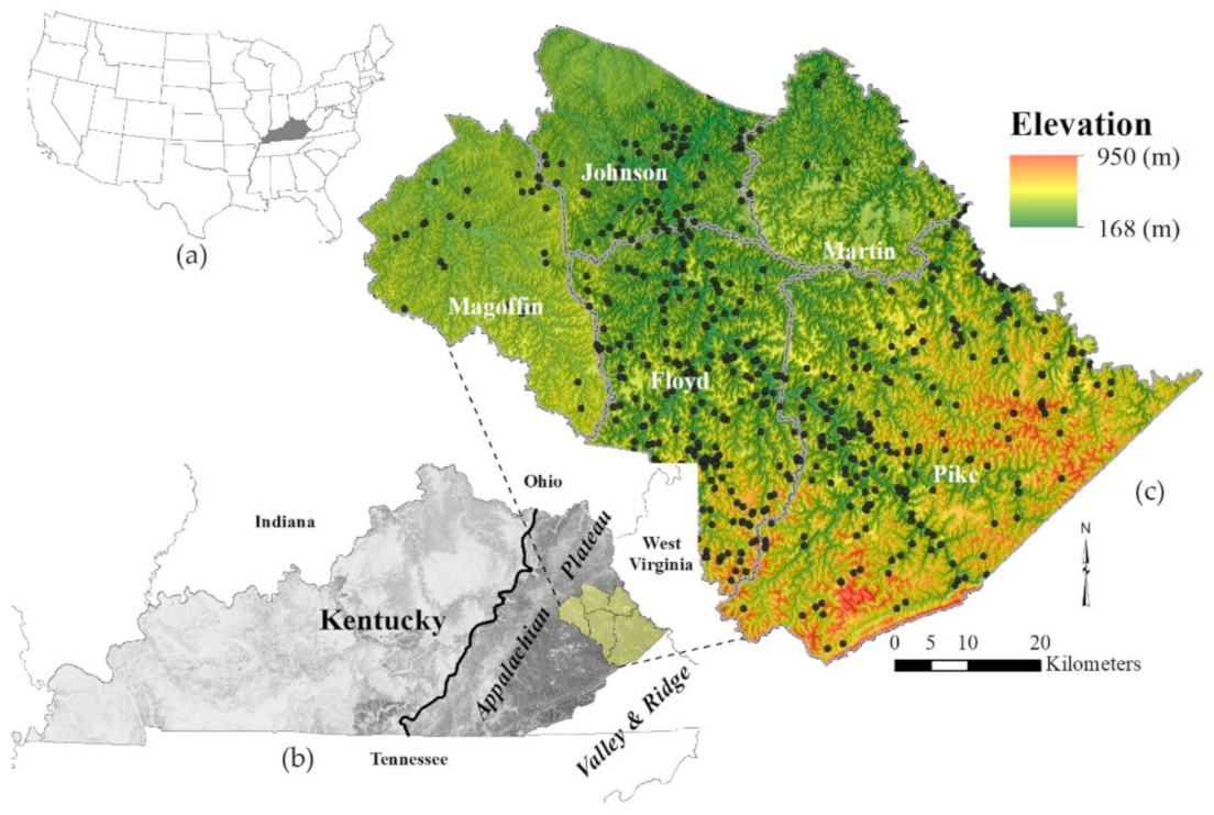
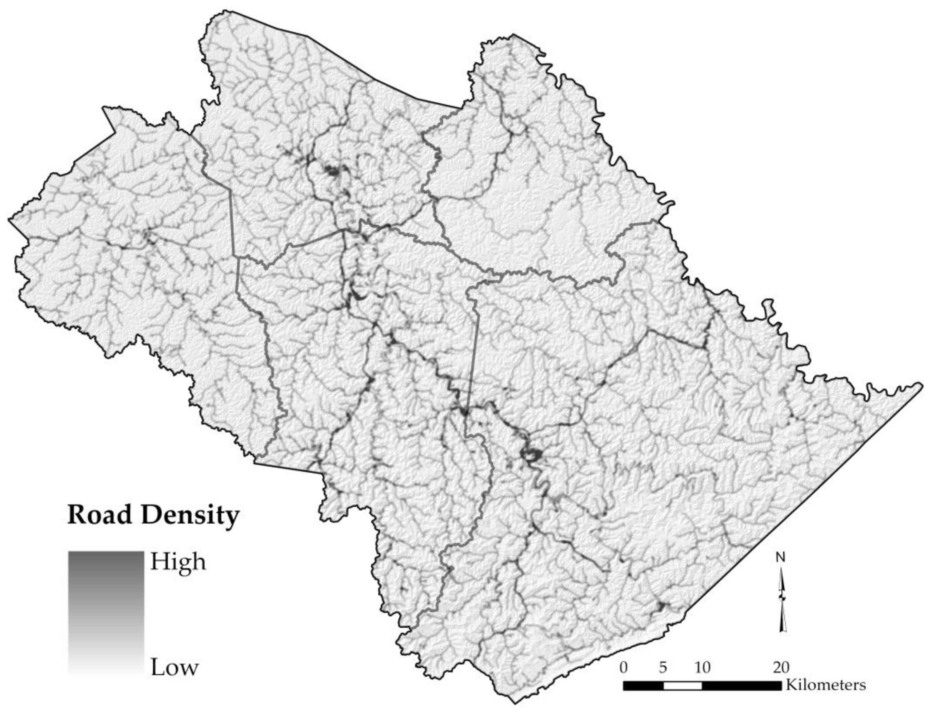
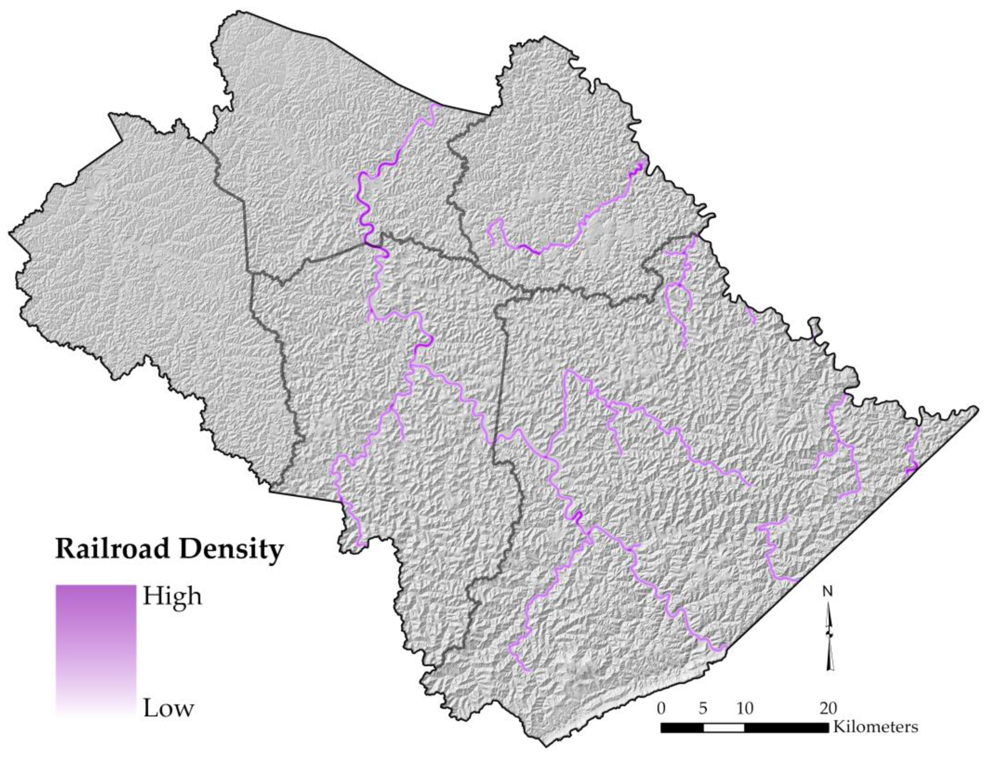
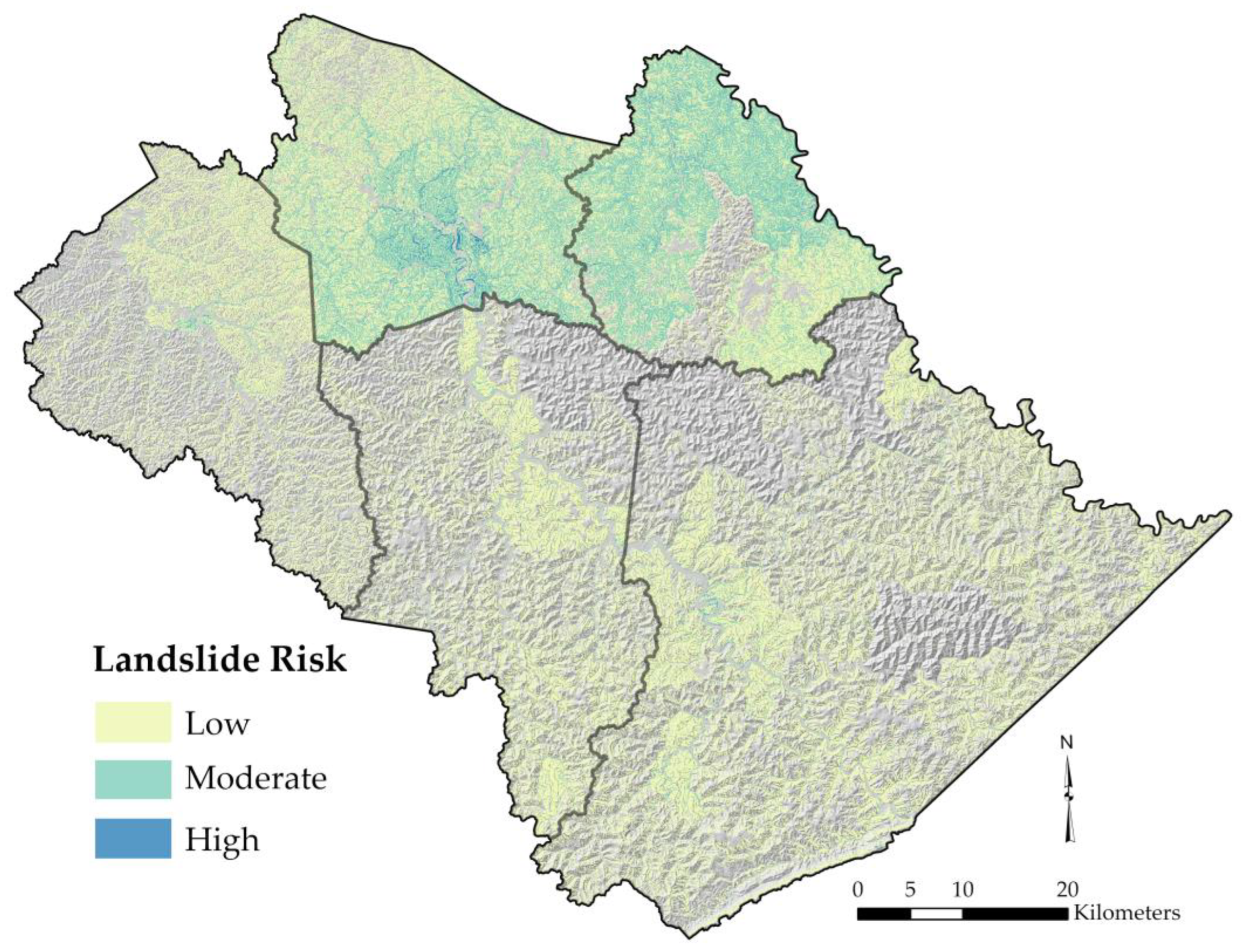
Our study focused on evaluating a technical range of model inputs with the need for practical, cost-effective solutions for stakeholders like emergency managers, first responders, local officials, and residents and communities at-risk from landslides. We produced two static socioeconomic risk maps that consider hazard data limitations, as well as limited vulnerability and consequence data, in five eastern Kentucky counties with chronic landslide problems. Both approaches leverage existing remote sensing data and generalized infrastructure and land-use data useful for estimating exposure and consequence. One approach uses a robust landslide inventory, 1.5 m airborne lidar digital elevation models (DEM), and lidar-derived geomorphic datasets to model landslide susceptibility [43]. High-resolution remote sensing data provides an opportunity to model relevant geomorphic conditions that lead to landslides at a regional scale.
Our second risk approach uses a coarse slope angle map sourced from global 30 m DEM as a hazard input in the risk equation. This model incorporates no landslide susceptibility data, simplified exposure data, but similar vulnerability and economic consequence data. The main purpose of the coarse, slope-based approach is to demonstrate the myriad of results possible at regional scale with limited quality data availability. Given our history of working with regional development groups, we also sought to determine levels on the quantitative risk assessment continuum that met the practical needs of stakeholders. While coarse slope-based models are not computationally intensive and are more readily accessible, we argue that further refinement of risk components creates more practical and uniform risk models while maintaining ease of access.
A practical and useful landslide risk assessment can be developed at a regional scale with limitations regarding hazard behavior and asset data. We reason that somewhere in between quantitative and qualitative risk assessments is a practical level, perhaps a model in which hazard and exposure data are well-established, yet still limited, compared to an advanced quantitative assessment. A static, geomorphic-based landslide hazard input, minimal to no vulnerability data, and consequence data constrained to economic loss will model a true risk assessment that is a useful, realistic combination of inputs. In fact, many approaches have effectively used a hazard input, yet are still limited with vulnerability and exposure data, often over-simplifying results. For example, the Federal Emergency Management Agency (FEMA) National Risk Index for 18 natural hazards, including landslides, leverages available source data for baseline risk for counties and census tracts [17]. These risk approaches can effectively connect data and modeling needs, computational requirements, and expert knowledge, which makes this approach practical at various scales.

2. Study Area

The study area comprises five counties in eastern Kentucky, USA (Magoffin, Johnson, Floyd, Martin, and Pike Counties) that form the Big Sandy Area Development District. The study area lies within the Appalachian Plateau, which is part of the larger Appalachian Basin northwest of the Valley and Ridge Province (Figure 1), characterized by steep hillsides with a mean slope angle of 24° to 25° [44]. Rainfall-triggered landslides (including translational landslides, slumps, creep, debris flows, and rockfalls) are a dominant erosional process creating significant direct and indirect costs in the region [9,45,46]. Infrastructure and buildings are generally restricted to narrow valley bottoms, with moderate amounts of development on steep hillsides and reclaimed coal mine sites. The Big Sandy Area Development District encompass 5,136 km2 with a population of 140, 215 people [47]. Four of the five counties of the area are recognized as economically distressed as defined by indicators such as high percentages in average unemployment and poverty rates [48]. The development district includes 2519 km of state-maintained, roads and 3443 km of locally maintained roads, and 419 km of privately maintained railroads.

2.1. Geology

Bedrock geology across most of eastern Kentucky consists of sequences of relatively flat-lying sedimentary rocks that include thin to thick beds of sandstone, shale, siltstone, coal, and underclay. The landscape is highly dissected, with narrow ridges and sinuous alluvial valleys. Deeply incised valleys range from long and narrow main stems to short bowl-shaped tributary catchments. Slopes are covered with colluvium ranging in thickness from 0.5 to 5 m. The colluvium is, in general, poorly sorted, fine to coarse loam with grain sizes that range from clay to medium-coarse boulders perhaps a meter in diameter [49]. Closely influenced by the lithology of the rocks below the soil, landslides in colluvium are commonly thin (<3 m) translational slides or thicker rotational slumps with both types being capable of developing into damaging debris flows or earth flows, especially on steep slopes [45,50,51].

2.2. Study Area Impact

The counties included in this study incur high landslide occurrence impacting several municipalities [45,52]. Historically, severe storm events with high-intensity and/or long-duration rainfall have triggered shallow, rapidly moving landslides, or remobilized existing slow-moving landslides, resulting in casualties and property damage in many parts of the Appalachian Plateau [53]. From 2015 to 2021, Kentucky received 11 presidential disaster declarations due to severe storms, flooding, and landslides (Table 1). These declarations allow public officials (FEMA in the U.S.) to exercise emergency powers to assess damage and preserve life and property following a disaster.
The estimated direct cost for landslides across Kentucky ranges from $10 to $20 million annually and has caused damage to homes, commercial property, and transportation infrastructure [45,54] (Figure 2). Indirect costs such as road closures, decreased property values, and utility interruption are potentially significant but are difficult to quantify. Figure 3 shows the study area roads that are classified by the cost of damage per state route based on transportation maintenance records from 2003 to 2009 for landslides and rockfalls [55]. These are only routine maintenance cost records and do not include large, expensive, geotechnical mitigation projects. Broad assessments of impacts such as these direct costs emphasize the need for subsequent, more robust, risk assessments.

3. Materials and Methods

We evaluated two quantitative approaches based on Equation (1).
Risk = Hazard × Vulnerability × Consequence
We define hazard as the likelihood a landslide will occur, vulnerability as the likelihood of elements at risk of having an adverse result to a landslide, and consequence as the economic or societal loss expected should a landslide affect the asset.
The first approach utilizes landslide susceptibility data as the landslide hazard input, vulnerability, and consequence data. The second approach uses a coarse (30 m) slope map as the hazard input along with simplified exposure data, specifically using U.S. Census Bureau block groups https://www.census.gov/data.html (accessed on 3 April 2020) for population input. Vulnerability remained the same in the risk calculation. The coarse, slope-based map comparison demonstrates the spectrum of results and sensitivity of quantitative risk calculation inputs.

3.1. Landslide Susceptibility Approach

3.1.1. Hazard Input

The hazard input is a landslide susceptibility map produced from a machine learning and logistic regression-based landslide susceptibility model described by Crawford and others [43]. The model combined two traditionally distinct machine-learning methods that complement each other to produce a susceptibility map. The susceptibility model is based on geomorphic variables slope, curvature, plan curvature, terrain roughness, and aspect from a 1.5 m lidar-derived regional digital elevation model and a detailed landslide inventory (N > 1054) for Magoffin County, Kentucky. The mean landslide area was 6400 m2, however specific slide type and age was not determined. An equal number of landslides (1) and non-landslides (0) made up the binary data set of variables. The bagged tree model predicts a weighted classification from the variables and ranks importance. The logistic regression model estimates the probability of landslide occurrence (that a raster cell is occupied, or might be occupied in the future, by a landslide) as a function of the statistical analysis and combination of geomorphic variable values (Figure 4). We found that eight variables were significant (p-value < 0.05) and the model performance evaluation by the receiver operating curve, area under the curve, was 0.83 [43]. Leveraging quality, high-resolution remote-sensing data including lidar, lidar-derived geomorphic datasets, and aerial photography allowed for a accurate and high-performance landslide susceptibility model, which we applied at the five-county regional scale.
We classified the landslide susceptibility results in GIS using equal interval classes, which is a data interval classification that works well with skewed data distribution (not normal distribution), focusing the high and low values and emphasizing the value to the rest of the map area. Equal interval will also allow a seamless uniform scheme across county boundaries. Table 2 shows the probability values, susceptibility classifications, percent area, and intersections with assets divided up by county. The buildings, roads, and railroads were expanded with a 15 m buffer during the intersection process to encompass a more realistic footprint of the asset.

3.1.2. Elements at Risk (Exposure and Assets)

We generated kernel density maps for major assets, defined as elements at risk potentially affected by landslides, in the area. We used population, roads, and railroads as exposure inputs in our risk models because they are critical datasets for determining socio-economic risk, but also measurable assets in terms of spatial extent and monetary value. A kernel density map is a smoothed raster estimation of the number of occurrences per unit area (density) of a point or line feature, produced by replacing each discrete point or line with a smooth continuous function and summing the results weighted by distance from the geographic point at which the density is being estimated. To generate the population kernel density map, we used the 2018 census block group population values [56] and building footprints. We divided the block group population value per centroid point of each building footprint (Figure 5). Although not all building footprints are inhabited homes, nor does the assigned value correspond with the true number of occupants, calculating a population density using a centroid of a building footprint assigned with a population provides a more realistic distribution of people than using the centroid of the block group (Figure 6). If we had generated a population kernel density map based on census block group data alone, with perhaps no buildings or roads in the area, that would create a much coarser map. The kernel density for roads and railroads was generated based on units of length of line per square map unit (Figure 7 and Figure 8). For each asset we used a search radius of 300 m (radius within which to calculate density) in the kernel density function. This search radius accounted for the true footprint of assets, which represents the adjacent property that may be at risk. Using a quartic kernel function for point (population) and line data (roads and railroads), the density at each output raster cell (pixel) is the units of the number of points per square map unit and units of length of line per square map unit, respectively [57].
We also included land class (developed and undeveloped) as an asset in our assessment to capture the threat of landslides that occur upslope on land that does have some value but is perhaps away from other assets in valley bottoms. To do so, we rasterized the polygon building footprints using a 15 m buffer, then reclassified the raster as developed and undeveloped land. All areas outside the building buffer were considered undeveloped, combining land classes woodland, cropland, and pasture as undeveloped. Buffering the buildings allowed us to include adjacent property and accurately define a larger area of developed land classification.

3.1.3. Asset Values

To assign the monetary values to the roads and railroads, we rasterized those assets by buffering the line data. Local roads received 6 m and 3 m buffers for county and private roads, respectively. State roads received a 9 m buffer and the U.S. highways received a 30 m buffer. Railroads received a 3 m buffer. We obtained economic value estimates for state roads, local roads, railroads, developed land, and undeveloped land from several government and industry sources (Table 3). The costs are considered recovery costs and not necessarily the market value of each asset. We determined the value of roads from the Kentucky Transportation Cabinet, which estimated the value of state-maintained roads through the Governmental Accounting Standards Board [58]. The methodology is based on cost-to-build values at the time and used construction costs categorized by two major costs factors, facility type (two-lane, multi-lane divided) and terrain type (Table 4). We determined values of railroads using a value of $1,000,000 to $2,000,000 per 1.6 km estimated by the Aberdeen Carolina and Western Railway [59]. Because of the wide range of values for railways, we used the more conservative $1 million value for this study.
We used developed land values from the U.S. Federal Housing Finance Agency [60]. We used properties that fell in the study area, a small sample (N = 26) focused in one county, to create an average of 0.1 hectare value as an estimation of property within the entire project area. We determined the undeveloped land values using data available from the University of Kentucky College of Agriculture and the United States Department of Agriculture [61,62]. Undeveloped land monetary values were averaged at $4500 per hectare. We converted the asset data to dollars per-pixel rasters for model input consistency. For example, dollars per hectare in land value was converted to a value per 3 m by 3 m pixel (Figure 9).

3.1.4. Vulnerability and Consequence

There are many aspects of landslide hazard vulnerability (including social, economic, physical, cultural, and environmental) that dictate vulnerability being degree of loss expressed as a scale of 0 (no loss) to 1 (total loss) [24,34,63]. Due to the lack of comprehensive vulnerability data such as landslide behavior and infrastructure resistance, we assumed a constant vulnerability value of 1, essentially a worst-case scenario for a degree of loss. The other component of our risk assessment is consequence. We define consequence as an estimate of the value of the elements at risk. The consequences in our risk assessment are categorized as societal (consideration of population and infrastructure exposure) and economic (consideration of the value of assets), therefore C is calculated in terms of the elements at risk and their economic value, used as cost per pixel.

3.2. Coarse, Slope-Based Approach

The slope-based risk input data differs from the susceptibility-based risk approach in three ways (Table 5). First, we used a publicly and globally available 30 m DEM acquired from the NASA Shuttle Radar Topography Mission [64]. We generated a slope map using the 30 m DEM to replace the lidar-based landslide susceptibility map as the hazard input. The slope map was resampled to 3 m cell resolution and scaled by the maximum value to compare. Second, the population asset data were generated from U.S. Census Bureau block groups https://www.census.gov/data.html (accessed on 3 April 2020), as opposed to the kernel density population map. The third difference is that the road, railroad, and land exposure raster maps were not included in the consequence component of the risk equation. However, these assets’ cost-per-pixel maps and cost data remained the same.

3.3. Risk Model Estimation

For both approaches, we used a risk equation incorporating hazard, vulnerability, and consequences to produce a socioeconomic landslide risk map (Equation (2)).
R = (H) × (V) × [(C1) + (C2) + (C3)]
where, H is the hazard (dimensionless), V is vulnerability (V = 1, no units), C is consequence, which is the economic value bins multiplied by binned population kernel density (C1), binned road kernel density (C2), and binned railroad kernel density (C3). The C component calculates a socio-economic consequence (unitless).
The consequence components are the elements at risk split into separate components, societal (kernel density maps) and economic (infrastructure and land monetary value maps). Asset values range from $4 to $45,454 per pixel (see Table 3 and Table 4). In order to maintain the influence of all asset data in the risk calculation, and to not skew risk towards the most expensive asset, we categorized the values of roads, railroads, and land class into order of magnitude bins with the highest being $10–100 k. Similarly, to avoid skew in kernel density population, we categorized the data into six commensurate bins, as opposed to order of magnitude bins because of the narrower range of density values compared to asset dollar values. These binned consequence elements are combined and then multiplied by the hazard and vulnerability value to calculate a risk (R) value for each raster.
The slope-based map estimation did not include the kernel density or land-use maps in the exposure component. The asset costs and cost-per-pixel map data remained the same. This change of using different hazard inputs and keeping the asset costs the same (while excluding the exposure maps) allows for a quality comparison between estimations and maps. The slope-based estimation is an example of a limited resource risk assessment and demonstrates a reality for many communities that lack robust model inputs.

4. Results

4.1. Susceptibility-Based Risk Map

All data inputs were normalized prior to calculating risk. Therefore, R in Equation (2) is unitless and we consider the result a risk factor score having a theoretical range of 0–1. We determined the risk classification using the standard deviation of the logarithm of the risk results because of the range of risk factor scores. The classification generated five classes; however, we excluded the lowest two classes because those areas are mostly stable ridgetops or valley bottoms (Table 6). The resulting three risk classifications applied to all counties are low, moderate, and high (Figure 10). The logarithm of the risk factor score creates a more practical, useable map classification, similar to a natural breaks classification. The areas not designated in a risk class (no color) could be moved into a risk classification if the hazard input data changed or development occurred.
Risk results indicate 64.1 percent of the study area is classified as moderate to high risk. In general, high concentrations of buildings, roads, and railroads that intersect, or are in the vicinity of, areas with high landslide susceptibility values, are classified as moderate or high risk (Figure 11). Hillslopes with little to no infrastructure are classified as low risk (mapped in yellow). High concentrations of buildings and roads along steep streambanks and below steep slopes are classified as high risk. We did not calculate values for areas with topographic slope angles < 3°. The risk maps do not consider scenario-based elements and should be considered static socioeconomic risk maps. As a final step, we resampled the risk maps with a 15 m radial smoothing window to reduce visual noise. The smoothing is a focal statistics function calculated in ArcGIS https://desktop.arcgis.com/en/arcmap/10.3/tools/spatial-analyst-toolbox/focal-statistics.htm (accessed on 4 May 2022) that uses a neighborhood operation to compute an output raster where the value for each output cell is a function of the values of all the input cells that are in a specified neighborhood around that location.

4.2. Slope-Based Risk Map

Compared to the susceptibility-based map, the coarse, slope-based map shows a less consistent distribution of risk and shows no or very little risk in many block groups (Figure 12). This difference partially hinges on the census block group population input. The primary differences in the slope-based maps include:
(1)
The census block group data outweighs the asset density to skew the risk distribution compared to the susceptibility-based map. The coarseness of the census block group data creates sharp and unrealistic risk boundaries. The modeled results show large areas with little risk and some blocks with no risk. These boundaries create inconsistency with how assets fall within risk classes.
(2)
A broad under-prediction at all classes relative to the susceptibility-based maps, particularly in less populated areas. In rural, sparsely populated areas, the moderate and high-risk classes are significantly reduced to low or no risk in the slope-based map. Risk in the low class dropped an average of 39 percent over all counties in the slope-based map.
(3)
Only two counties showed an increase in the moderate risk class, 16 and 22 percent in Johnson and Martin counties, respectively, which contains some of the most populated census blocks. However, this creates high risk surrounding buildings, roads, and stream banks inconsistent.
(4)
Few building footprints adjacent to steep high-hazard slopes, particularly in the narrow valleys and catchments, are classified as moderate or high risk. Classification of risk along roads, particularly local roads, is much less consistent compared to the susceptibility-based map. Very few local roads fall within the high-risk category.
(5)
Because of the slope input, the map shows less over-prediction compared to the susceptibility-based map at congested valley bottoms or engineered embankments. These small, high-density areas of roads, railroads, and buildings are not likely to be at risk.
Using a slope map derived from a 30 m DEM and the coarse U.S. Census Bureau block group-based population input data makes this map less consistent overall and generally under-represents risk. (Figure 13, Figure 14 and Figure 15). The slope map input creates less emphasis on open land risk, except in the more populated block groups, however, this approach could be used to guide a broad risk assessment at a state or national scale, but we demonstrate that perhaps a minor GIS task change that improves risk equation inputs does make a practical difference in map quality.

5. Discussion

The primary drawback for both quantitative and qualitative risk assessments is based on relevant degrees of data limitations and complex environmental conditions, and the uncertainties they introduce. Most advanced landslide hazard assessments require landslide frequency and run-out data that does not exist. Similarly, landslide vulnerability and consequence data regarding building types, road infrastructure, and personal safety is virtually non-existent in most places in the world. However, understanding that a range of quantitative risk assessments is a continuum that includes advanced, site-specific models to over-simplified modelling techniques is the foundation of developing a risk assessment that is useful for landslide-prone communities. We demonstrate a variety of methods, from conventional risk estimations to sparse, yet resourceful risk model inputs can effectively address data limitations and produce quality maps.
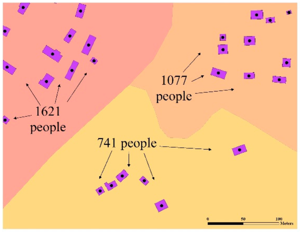
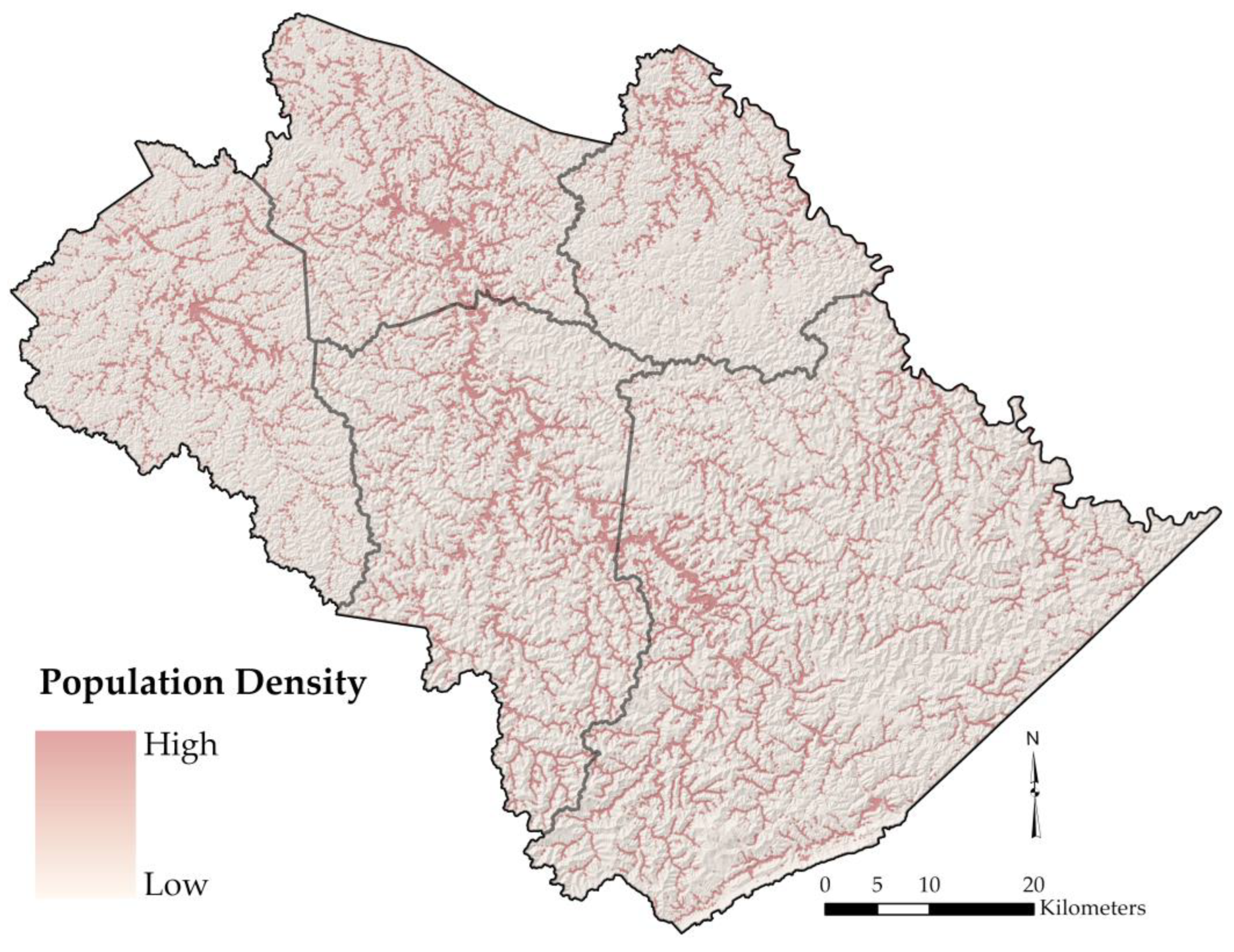
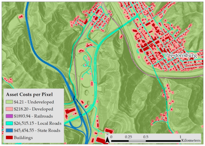
Our models emphasize a regional scale, limited data approach that provides risk information for imposing risk evaluation and mitigation strategies for communities. The hazard input (landslide susceptibility) to our risk equation highlights the importance of existing deposits that have a moderate to a high probability of subsequent movement and highlight other parts of the slope that do not necessarily show obvious landslide activity but are classified, nonetheless. The hazard input is limited regarding landslide type and behavior (extent or runout), however using static probability serves as a critical risk input. We obtained the economic values from various sources, and all were generalized as total values for the elements in question. Developed and undeveloped land values were determined from a small sample of property values. This analysis lacks data on other highly vulnerable elements, such as powerlines, water lines, and sewerage lines, therefore these elements are not included in the risk assessment. Population considerations did not include where populations would be at any given moment. Vulnerability was assumed at the maximum value (1), which is not likely the case uniformly across the study area. We submit that using a vulnerability value of 1, combats an underestimating of landslide hazard impacts and the often-related reduced awareness and concern [65].
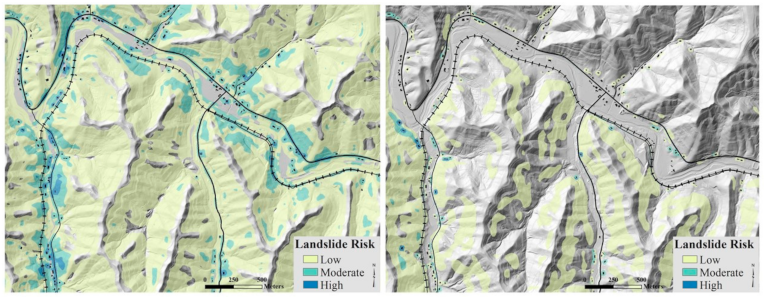
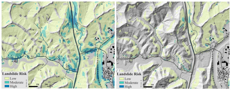
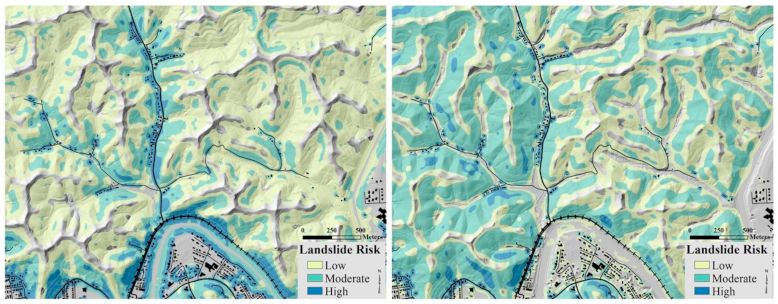
Our risk calculation and map derived from a coarse slope-based hazard input recognizes similarities in risk distribution at a regional scale, but also highlight the need for further evaluation of over-and under-predicted risk in several areas. These comparisons assume that our susceptibility-based landslide risk map is a strong model primarily because of the landslide susceptibility input, thus better constraining the areas vulnerable to landslides. A slope-based hazard input, limited exposure and consequence data, and limited computing power are a reality for developing countries striving for risk evaluation and implementation. The susceptibility map input is a superior input to slope angle, but minor GIS tasks (such as improving on census block data or how exposure is quantified) can significantly improve the risk calculation and results that make a practical difference in map quality.
Because we developed a socio-economic approach to risk, a recognition of how changing conditions and opportunities could impact community resilience in the long term need to be considered in future assessments. Additional data sets to consider in future risk mapping may include property value administrator data, traffic counts, cell phone locational data, geology, updated land class maps, and time-dependent rainfall. National Oceanic and Atmospheric Administration differenced 30-year averages (1991–2020 minus 1981–2010) which indicated Kentucky has experienced an increase in annual precipitation change across the state that ranges from 3–12% [66]. Increased precipitation will translate to more landslides and increased risk. Incorporating precipitation data, rainfall triggering thresholds, and other related climate change factors may also improve risk assessments in the future.
Considering the variability in methods for landslide risk, establishing the utility of model and map results, in conversation with local stakeholders, is critical. Regardless of the robustness of data availability and model inputs, landslide risk mapping can provide baseline information for all stakeholders that show economic benefits, improves public safety, and builds trust. Our results contain data to inform mitigation strategies that could support building and infrastructure assessment, land-use planning, event awareness, response, and recovery actions for communities in the region.

6. Conclusions

We evaluated a susceptibility-based landslide risk map and a more limited, slope-based approach in order to emphasize how minor changes in data quality can improve landslide risk assessments. Minor changes in the hazard and vulnerability inputs result in significant changes in the quality and applicability of risk maps. All approaches and inputs of regional-scale landslide risk assessments have limitations and a recognition of data resources and the quality of model inputs allows for comparison of map results that can be used by practitioners and communities to mitigate landslide hazards and reduce risk.
Using different hazard inputs (landslide susceptibility versus slope angle), exposure data, and associated economic value of assets in a risk equation, we generated two landslide risk maps for five counties in a landslide-prone portion of eastern Kentucky. We used a logistic regression-based landslide susceptibility model as the hazard input. The elements at risk included population, road, railroad, and land class inputs, along with associated asset costs (consequence). The vulnerability input was assumed to be (1), modelling a total loss. For the slope-based map, the vulnerability remained (1) and the road, railroad, and land exposure asset raster maps were not included in the consequence component of the risk equation. However, these assets’ cost-per-pixel maps and cost data remained the same.
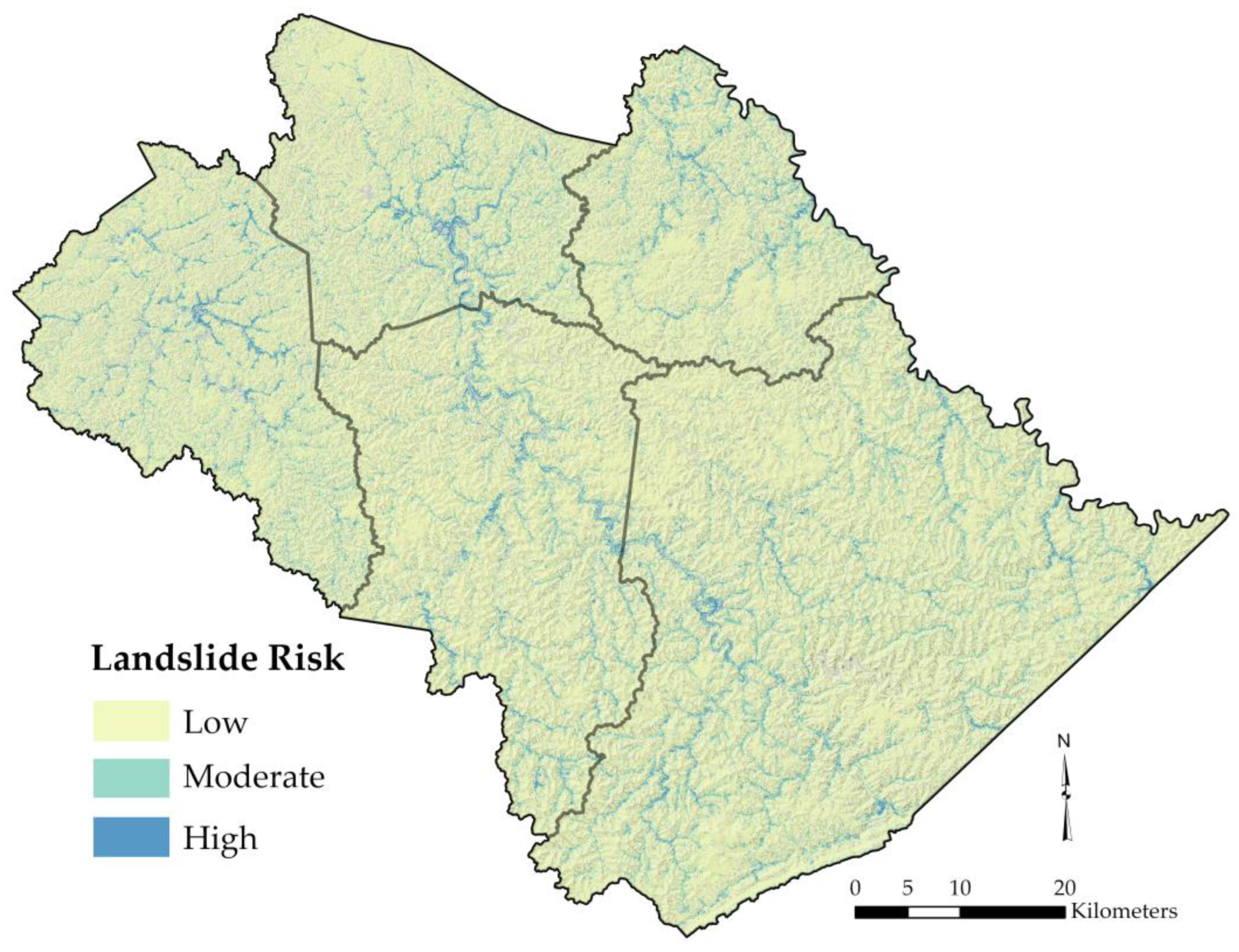
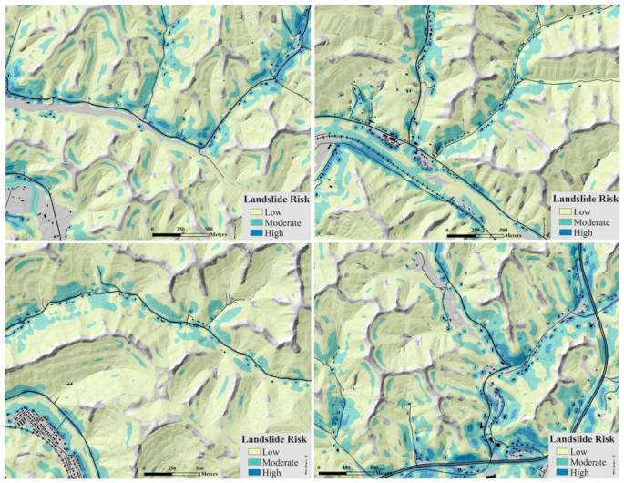
The susceptibility-based map indicates 64.1 percent of the study area is classified has moderate to high risk, with assets closer to high hazard areas being reliably highlighted as moderate to high risk. The map effectively highlights high-risk road segments, which is helpful to emergency managers, first responders, and local officials who need to communicate the threat of landslides. Broad, wide-open hillslopes and ridges with little to no infrastructure or other elements at risk are classified as low risk. Because of our asset density and hazard input (landslide susceptibility), the model over-predicted risk in some areas (compared to the slope-based map) particularly valley bottoms with dense areas of buildings or roads that are in close proximity to a toe slope or engineered embankment. These areas are mostly flat and have little correlated hazard.
The more data-limited risk assessment used a coarse (30-m) slope input and U.S. Census block group-derived population data, resulting in much less consistent distribution of a risk factor score. The map shows sharp boundaries between areas with moderate and high-risk and large areas of very low risk. These boundaries are coarse renderings of how buildings, roads, and railroads fall within risk classifications. Although identification of risk classes for local scale areas is possible with the slope-based map, the utility is limited for a broad five-county area.

Author Contributions

Conceptualization, M.M.C., J.M.D., W.C.H. and Z.W.; methodology, M.M.C., J.M.D., H.J.K. and Y.Z.; software, M.M.C., J.M.D. and Y.Z.; formal analysis, M.M.C., J.M.D., H.J.K., W.C.H. and Y.Z.; investigation, M.M.C., J.M.D. and W.C.H.; writing—original draft preparation, M.M.C.; writing—review and editing, J.M.D., H.J.K., W.C.H., Y.Z., Z.W. and L.S.B.; supervision, W.C.H., Z.W. and L.S.B.; project administration, M.M.C.; funding acquisition, M.M.C. All authors have read and agreed to the published version of the manuscript.

Funding

This work was supported by the Federal Emergency Management Agency Pre-Disaster Mitigation Grant Program (PDMC-PL-04-KY-2017-002).

Data Availability Statement

The Kentucky Geological Survey landslide inventory database (Crawford, 2022) is available here, https://uknowledge.uky.edu/kgs_data/7/ (accessed on 3 April 2020). The landslide susceptibility maps for the study are can be viewed here, https://kgs.uky.edu/kygeode/geomap/ (accessed on 3 April 2020).

Acknowledgments

We would like to thank Nick Grinstead from the University of Kentucky Martin School of Public Policy and Administration for grant assistance and logistics, Rachel Noble-Varney of the Kentucky Geological Survey for thorough manuscript reviews, and officials with the Big Sandy Area Development District of Kentucky for project support.

Conflicts of Interest

The authors declare they have no competing financial interests or personal relationships that could be conflicts of interest.

References

  1. Schuster, R.L. Socioeconomic significance of landslides. In Landslides Investigation and Mitigation, Special Report 247; Turner, A.K., Schuster, R.L., Eds.; Transportation Research Board, National Research Council: Washington, DC, USA, 1996; pp. 12–35. [Google Scholar]
  2. Crozier, M.J. Deciphering the effect of climate change on landslide activity: A review. Geomorphology 2010, 124, 260–267. [Google Scholar] [CrossRef]
  3. Anderson, M.G.; Holcombe, E. Community-Based Landslide Risk Reduction: Managing Disasters in Small Steps; World Bank Publications: Washington, DC, USA, 2013; 404p. [Google Scholar]
  4. Corominas, J.; van Westen, C.; Frattini, P.; Cascini, L.; Malet, J.P.; Fotopoulou, S.; Catani, F.; Van Den Eeckhaut, M.; Mavrouli, O.; Agliardi, F.; et al. Recommendations for the quantitative analysis of landslide risk. Bull. Eng. Geol. Environ. 2014, 73, 209–263. [Google Scholar] [CrossRef] [Green Version]
  5. Ludwig, K.A.; Ramsey, D.W.; Wood, N.J.; Pennaz, A.B.; Godt, J.W.; Plant, N.G.; Luco, N.; Koenig, T.A.; Hudnut, K.W.; Davis, D.K.; et al. Science for a Risky World—A U.S. Geological Survey Plan for Risk Research and Applications; U.S. Geological Survey Circular 1444; USGPO: Washington, DC, USA, 2018; 57p. [CrossRef] [Green Version]
  6. Gariano, S.L.; Guzzetti, F. Landslides in a changing climate. Earth-Sci. Rev. 2016, 162, 227–252. [Google Scholar] [CrossRef] [Green Version]
  7. Froude, M.J.; Petley, D.N. Global fatal landslide occurrence from 2004 to 2016. Nat. Hazards Earth Syst. Sci. 2018, 18, 2161–2181. [Google Scholar] [CrossRef] [Green Version]
  8. Sim, B.S.; Lee, M.L.; Wong, S.Y. A review of landslide acceptable risk and tolerable risk. Geoenvironmental Disasters 2022, 9, 1–17. [Google Scholar] [CrossRef]
  9. Mirus, B.B.; Jones, E.S.; Baum, R.L.; Godt, J.W.; Slaughter, S.; Crawford, M.M.; Lancaster, J.; Stanley, T.; Kirschbaum, D.B.; Burns, W.J.; et al. Landslides across the USA: Occurrence, susceptibility, and data limitations. Landslides 2020, 17, 2271–2285. [Google Scholar] [CrossRef]
  10. Keaton, J.R.; Roth, R.J., Jr. Mapping landslides for the insurance industry–lessons from earthquakes. In Proceedings of the EUROENGEO, the 2nd European Conference of International Association for Engineering Geology, Madrid, Spain, 9 June 2008; Volume 15, p. 19. [Google Scholar]
  11. Guinau, M.; Pallas, R.; Vilaplana, J.M. A feasible methodology for landslide susceptibility assessment in developing countries: A case-study of NW Nicaragua after Hurricane Mitch. Eng. Geol. 2005, 80, 316–327. [Google Scholar] [CrossRef]
  12. Papathoma-Köhle, M.; Kappes, M.; Keile, M.; Glade, T. Physical vulnerability assessment for alpine hazards: State of the art and future needs. Nat. Hazards 2011, 58, 645–680. [Google Scholar] [CrossRef]
  13. IUGS Working Group on Landslides; Committee on Risk Assessment. Quantitative assessment for slopes and landslides—The state of the art. In Landslide Risk Assessment, Proceedings of the Workshop on Landslide Risk Assessment, Honolulu, HI, USA, 19–21 February 1997; Cruden, D.M., Fell, R., Eds.; Balkema: Rotterdam, The Netherlands, 1997; pp. 3–12. [Google Scholar]
  14. VanDine, D.F. Landslide hazard and risk assessments for small projects, preliminary studies and emergency response. In Landslide Risk Assessment, Proceedings of the International Workshop on Landslide Risk Assessment, Honolulu, HI, USA, 19–21 February 1997; Cruden, D.M., Fell, R., Eds.; Balkema: Rotterdam, The Netherlands, 1997; 371p. [Google Scholar]
  15. Varnes, D.J. Landslides Hazard Zonation: A Review of Principles and Practice; UNESCO: Paris, France, 1984; 63p.
  16. Papathoma-Köhle, M.; Neuhäuser, B.; Ratzinger, K.; Wenzel, H.; Dominey-Howes, D. Elements at risk as a framework for assessing the vulnerability of communities to landslides. Nat. Hazards Earth Syst. Sci. 2007, 7, 765–779. [Google Scholar] [CrossRef]
  17. Zuzak, C.; Goodenough, E.; Stanton, C.; Mowrer, M.; Ranalli, N.; Kealey, D.; Rozelle, J. National Risk Index Technical Documentation; Federal Emergency Management Agency: Washington, DC, USA, 2021; 411p. Available online: https://www.fema.gov/sites/default/files/documents/fema_national-risk-index_technical-documentation.pdf (accessed on 31 August 2021).
  18. Crozier, M.J.; Glade, T. Landslide hazard and risk: Issues, concepts, approaches. In Landslide Hazard and Risk; Glade, T., Anderson, M.A., Crozier, M.J., Eds.; Wiley: Chichester, UK, 2005; pp. 1–40. [Google Scholar]
  19. Fell, R.; Ho, K.K.S.; Lacasse, S.; Leroi, E. A framework for landslide risk assessment and management. In Landslide Risk Management; Hungr, O., Fell, R., Couture, R., Eberhardt, E., Eds.; Taylor and Francis: London, UK, 2005; pp. 3–26. [Google Scholar]
  20. Remondo, J.; Bonachea, J.; Cendrero, A. Quantitative landslide risk assessment and mapping on the basis of recent occurrences. Geomorphology 2008, 94, 496–507. [Google Scholar] [CrossRef]
  21. Kappes, M.S.; Papathoma-Köhle, M.; Keiler, M. Assessing physical vulnerability for mult-hazards using an indicator-based methodology. Appl. Geogr. 2012, 32, 577–590. [Google Scholar] [CrossRef]
  22. Lee, E.M. Landslide risk assessment: The challenge of communicating uncertainty to decision-makers. Q. J. Eng. Geol. Hydrogeol. 2015, 49, 21–35. [Google Scholar] [CrossRef]
  23. Strouth, A.; McDougall, S. Societal risk evaluation for landslides: Historical synthesis and proposed tools. Landslides 2021, 18, 1071–1085. [Google Scholar] [CrossRef]
  24. Uzielli, M.; Nadim, F.; Lacasse, S.; Kaynia, A.M. A conceptual framework for quantitative estimation of physical vulnerability to landslides. Eng. Geol. 2008, 102, 251–256. [Google Scholar] [CrossRef]
  25. Van Westen, C.J.; van Asch, T.W.J.; Soeters, R. Landslide hazard and risk zonation–why is it still so difficult? Bull. Eng. Geol. Environ. 2006, 65, 167–184. [Google Scholar] [CrossRef]
  26. Wu, T.H.; Tang, W.H.; Einstein, H.H. Landslide hazard and risk assessment. In Landslides Investigation and Mitigation; Turner, A.K., Schuster, R.L., Eds.; Special Report 247; Transportation Research Board, National Research Council: Washington, DC, USA, 1996; pp. 106–118. [Google Scholar]
  27. Finlay, P.J.; Fell, R. Landslides: Risk perception and acceptance. Can. Geotech. J. 1997, 34, 169–188. [Google Scholar] [CrossRef]
  28. Leroi, E. Landslide risk mapping: Problems, limitations and developments. In Landslide Risk Assessment, Proceedings of the International Workshop on Landslide Risk Assessment, Honolulu, HI, USA, 19–21 February 1997; Cruden, D.M., Fell, R., Eds.; Balkema: Rotterdam, The Netherlands, 1997; pp. 239–250. [Google Scholar]
  29. Chowdhury, R.; Flentje, P. Uncertainties in rainfall-induced landslide hazard. Q. J. Eng. Geol. Hydrogeol. 2022, 35, 61–69. [Google Scholar] [CrossRef] [Green Version]
  30. Calvello, M.; Papa, M.N.; Pratschke, J.; Crescenzo, M.N. Landslide risk perception: A case study in Southern Italy. Landslides 2016, 13, 349–360. [Google Scholar] [CrossRef]
  31. Li, Z.; Nadim, F.; Huang, H.; Uzielli, M.; Lacasse, S. Quantitative vulnerability estimation for scenario-based landslide hazards. Landslides 2010, 7, 125–134. [Google Scholar] [CrossRef]
  32. Guillard-Gonçalves, C.; Zêzere, J. Combining social vulnerability and physical vulnerability to analyze landslide risk at the municipal scale. Geosciences 2018, 8, 294–317. [Google Scholar] [CrossRef] [Green Version]
  33. Haneberg, W.C.; Johnson, S.E.; Gurung, N. Response of the Laprak, Nepal, landslide to the 2015 Mw 7.8 Gorkha earthquake. Nat. Hazards 2022, 111, 567–584. [Google Scholar] [CrossRef]
  34. Caleca, F.; Tofani, V.; Segoni, S.; Raspini, F.; Rosi, A.; Natali, M.; Catani, F.; Casagli, N. A methodological approach of QRA for slow-moving landslides at a regional scale. Landslides 2022, 19, 1539–1561. [Google Scholar] [CrossRef] [PubMed]
  35. Rossi, M.; Guzzetti, F.; Salvati, P.; Donnini, M.; Napolitano, E.; Bianchi, C. A predictive model of societal landslide risk in Ital. Earth-Sci. Rev. 2019, 196, 102849. [Google Scholar] [CrossRef]
  36. Lan, H.; Tian, N.; Li, L.; Wu, Y.; Macciotta, R.; Clague, J.J. Kinematic-based landslide risk management for the Sichuan-Tibet Grid Interconnection Project (STGIP) in China. Eng. Geol. 2022, 308, 106823. [Google Scholar] [CrossRef]
  37. Catani, F.; Casagli, N.; Ermini, L.; Righini, G.; Menduni, G. Landslide hazard and risk mapping at catchment scale in the Arno River basin. Landslides 2005, 2, 329–342. [Google Scholar] [CrossRef]
  38. Dai, F.C.; Lee, C.F.; Ngai, Y.Y. Landslide risk assessment and management: An overview. Eng. Geol. 2002, 64, 65–87. [Google Scholar] [CrossRef]
  39. Puissant, A.; Eeckhaut, M.; Malet, J.P.; Maquaire, O. Landslide consequence analysis: A region-scale indicator-based methodology. Landslides 2014, 11, 843–858. [Google Scholar] [CrossRef]
  40. Abella, E.A.C.; Van Westen, C.J. Generation of landslide risk index map for Cuba using spatial multi-criteria evaluation. Landslides 2007, 4, 311–325. [Google Scholar] [CrossRef] [Green Version]
  41. Lee, E.M.; Jones, D.K.C. Landslide Risk Assessment; Thomas Telford: London, UK, 2004. [Google Scholar]
  42. Fell, R.; Corominas, J.; Bonnard, C.; Cascini, L.; Leroi, E.; Savage, W.Z. Guidelines for landslide susceptibility hazard, and risk zoning for land use planning. Eng. Geol. 2008, 102, 99–111. [Google Scholar] [CrossRef]
  43. Crawford, M.M.; Dortch, J.M.; Koch, H.J.; Killen, A.A.; Zhu, J.; Zhu, Y.; Bryson, L.S.; Haneberg, W.C. Using landslide-inventory for a combined bagged-trees and logistic regression approach to landslide susceptibility in eastern Kentucky, United States. Q. J. Eng. Geol. Hydrogeol. 2021, 54. [Google Scholar] [CrossRef]
  44. Outerbridge, W.F. The Logan Plateau, a Young Physiographic Region in West Virginia, Kentucky, Virginia, and Tennessee; Bulletin 1620; USGPO: Washington, DC, USA, 1987; 19p.
  45. Crawford, M.M. Kentucky Geological Survey Landslide Inventory: From Design to Application; Information Circular 31, Series 12; Kentucky Geological Survey: Lexington, KY, USA, 2014; 18p. [Google Scholar]
  46. McDowell, R.C. Geology of Kentucky—A Text to Accompany the Geologic Map of Kentucky; U.S. Geological Survey Professional Paper 1151-H; USGPO: Washington, DC, USA, 1986.
  47. U.S. Census Bureau, 2020, County Population Totals. Available online: https://www.census.gov/programs-surveys/popest/technical-documentation/research/evaluation-estimates/2020-evaluation-estimates/2010s-counties-total.html (accessed on 22 February 2022).
  48. Appalachian Regional Commission, Classifying Economic Distress in Appalachian Counties. Available online: https://www.arc.gov/classifying-economic-distress-in-appalachian-counties/ (accessed on 21 February 2022).
  49. Blair, T.C.; McPherson, J.G. Grain-size and textural classification of coarse sedimentary particles. J. Sediment. Res. 1999, 69, 6–19. [Google Scholar] [CrossRef]
  50. Outerbridge, W.F. Relation between landslides and bedrock in the central Appalachian Plateaus. In Landslides of Eastern North America; Schultz, A.P., Southworth, C.S., Eds.; U.S. Geological Survey Circular 1008; USGPO: Washington, DC, USA, 1987; 43p. [Google Scholar]
  51. Turner, A.K. Colluvium and talus. In Landslides Investigation and Mitigation; Turner, A.K., Schuster, R.L., Eds.; Special Report 247; Transportation Research Board, National Research Council: Washington, DC, USA, 1996; pp. 525–554. [Google Scholar]
  52. Crawford, M.M. Kentucky Geological Survey landslide inventory (2022-01). Ky. Geol. Surv. Res. Data 2022. [Google Scholar] [CrossRef]
  53. Wieczorek, G.F.; Mossa, G.S.; Morgan, B.A. Regional debris-flow distribution and preliminary risk assessment from severe storm events in the Appalachian Blue Ridge Province, USA. Landslides 2004, 1, 53–59. [Google Scholar] [CrossRef]
  54. Wold, R.L., Jr.; Jochim, C.L. Landslide Loss Reduction: A Guide for State and Local Government Planning; Earthquake Hazards Reduction Series 52; Federal Emergency Management Agency: Washington, DC, USA, 1989; 50p.
  55. Overfield, B.L.; Carey, D.I.; Weisenfluh, G.A.; Wang, R.; Crawford, M.M. The Geologic Context of Landslide and Rockfall Maintenance Costs in Kentucky; Report of Investigations, 34, Series 12; Kentucky Geological Survey: Lexington, KY, USA, 2015; 54p. [Google Scholar]
  56. U.S. Census Bureau, 2014–2018 American Community Survey 5-Year Estimates. Available online: https://www.census.gov/programs-surveys/acs/technical-documentation/code-lists.2018.html (accessed on 22 February 2022).
  57. Silverman, B.W. Density Estimation for Statistics and Data Analysis; Routledge: London, UK, 1998. [Google Scholar] [CrossRef]
  58. Governmental Accounting Standards Board, Summary of Statement No. 34. Available online: http://www.gasb.org/st/summary/gstsm34.html (accessed on 15 September 2021).
  59. Aberdeen Carolina and Western Railway. Available online: http://www.acwr.com/economic-development/railroads-101/rail-siding-costs (accessed on 15 September 2021).
  60. Davis, M.A.; Larson, W.D.; Oliner, S.D.; Shui, J. The price of residential land for counties, ZIP codes, and census tracts in the United States. J. Monet. Econ. 2020, 118, 413–431. [Google Scholar] [CrossRef]
  61. Halich, G.; Pulliam, P. Land Value and Cash Rent Survey; AEC-97; Cooperative Extension Service, College of Agriculture, University of Kentucky; University of Kentucky: Lexington, KY, USA, 2013. [Google Scholar]
  62. U.S. Department of Agriculture. Land Values 2019 Summary, National Agricultural Statistics Service. 2019. Available online: https://www.nass.usda.gov/Publications/Todays_Reports/reports/land0819.pdf (accessed on 27 May 2020).
  63. Glade, T. Vulnerability assessment in landslide risk analysis. Erde 2003, 134, 123–146. [Google Scholar]
  64. Shuttle Radar Topography Mission (SRTM), 1 Arc-Second Global. Available online: https://doi.org/10.5066/F7PR7TFT (accessed on 7 March 2022).
  65. Althuwaynee, O.F.; Pradhan, B. Semi-quantitative landslide risk assessment using GIS-based exposure analysis in Kuala Lumpur City. Geomat. Nat. Hazards Risk 2016, 8, 706–732. [Google Scholar] [CrossRef] [Green Version]
  66. Arguez, A.; Durre, I.; Applequist, S.; Vose, R.S.; Squires, M.F.; Yin, X.; Heim, R.R., Jr.; Owen, T.W. NOAA’s 1981–2010 US climate normals: An overview. Bull. Am. Meteorol. Soc. 2012, 93, 1687–1697. [Google Scholar] [CrossRef]
Figure 1. Map showing the locations of Kentucky, USA (a), the eastern Big Sandy Area Development District (b), and elevation map of the counties in the district (c). Black dots are documented landslides from the Kentucky Geological Survey inventory database.
Remotesensing 14 06246 g001
Figure 2. Landslide head scarp threatening a home in Floyd County (upper left, photo credit Matt Crawford), landslide on road in Johnson County (upper right, photo credit Johnson County Emergency Management), and a debris flow that caused a train derailment in Pike County (bottom, photo credit Pike County Emergency Management).
Remotesensing 14 06246 g002
Figure 3. Landslide and rockfall costs per state route in the Big Sandy Area Development District, eastern Kentucky, USA. Costs are in U.S. dollars from 2003 to 2009. Map generated from data in [55].
Remotesensing 14 06246 g003
Figure 4. Landslide susceptibility in the Big Sandy Area Development District, eastern Kentucky, USA. County boundaries are shown in gray. The map data serves as the hazard input to the risk calculation. Susceptibility is calculated as a probability of occurrence derived from a geomorphic-based, logistic regression model.
Remotesensing 14 06246 g004
Figure 5. Example area showing three different U.S. census block groups and their total population, divided among the centroids (black dots) of building footprints (purple polygons) to generate the population kernel density map.
Remotesensing 14 06246 g005
Figure 6. Kernel density map of population for the Big Sandy Area Development District. The low to high range of density classification represents the units of number of points per square map unit.
Remotesensing 14 06246 g006
Figure 7. Kernel density map of state and local roads for the Big Sandy Area Development District. The low to high range of density classification represents the units of length of line per one square map unit.
Remotesensing 14 06246 g007
Figure 8. Kernel density map of railroads for the Big Sandy Area Development District. The low to high range of density classification represents the units of length of line per one square map unit.
Remotesensing 14 06246 g008
Figure 9. Cost-per-pixel map of part of Floyd County in the Big Sandy Area Development District. Values are in U.S. dollars.
Remotesensing 14 06246 g009
Figure 10. Landslide risk for the Big Sandy Area Development District. County boundaries are shown in gray.
Remotesensing 14 06246 g010
Figure 11. Risk map examples, Magoffin County (upper left), Pike County (upper right), Floyd County (lower left), and Johnson County (lower right). Black lines are roads, black polygons are buildings, and hatched lines are railroads.
Remotesensing 14 06246 g011
Figure 12. Slope-based risk map of the Big Sandy Area Development District. A coarse slope map as the hazard input and population data generated from U.S. Census block groups models an inconsistent risk distribution, creating stark boundaries of risk classes. Counties models were generated individually, those with smaller population ranges show high-skewing results. County boundaries are shown in gray.
Remotesensing 14 06246 g012
Figure 13. Comparison of the susceptibility-based map (left) and slope-based risk map (right) for part of Pike County. The block group-based population data and coarse slope map input creates stark boundaries in risk classes (right). The northeast portion of the slope-based map (right) shows how low population removes all risk, except for areas directly adjacent to buildings roads. While not inaccurate, the remaining area shows that more highly populated block-groups do not have such stark skews.
Remotesensing 14 06246 g013
Figure 14. Comparison of the susceptibility-based map (left) and slope-based map (right) in part of Floyd County. The block group-based population data and coarse slope map input creates stark boundaries in risk classes (right). Compared to the map on the left, under prediction is apparent in the slope-based map (right), and population block-group data skews the model results between boundaries.
Remotesensing 14 06246 g014
Figure 15. Comparison of the susceptibility-based map (left) and slope-based map (right) in populated part of Johnson County. Relatively large population differences in block group-based population create over prediction of risk at the block-group boundaries (right).
Remotesensing 14 06246 g015
Table 1. Rainfall and related FEMA-designated presidential disaster declarations in Kentucky (KY) from 2015 to 2021. Documented landslides from the Kentucky Geological Survey inventory database.
DatesRainfallDisaster DeclarationsLandslides Documented
March 201580 mm on March 3–4 over much of SE KY, followed by 50 to 200 mm in April4Over 100 landslides documented for the year
2016Average of 1285 mm statewide1Approximately 60 landslides documented
Winter 2018 data
125 to 250 mm of 14-day observed rainfall ending February 18 across SE KY2Approximately 43 landslides documented from December to March
2019An average of 1525 mm statewide1Approximately 153 landslides documented for the year
Winter-Spring 202050 to150 mm from February 4–6 in SE KY, 66 mm in 12 h in parts of two counties, 200 to 380 mm from January 1 to February 11, 25 to 75 mm followed in 24 h on April 13, and 25 to 100 mm on May 19–20.2Approximately 123 landslides documented for the year, 30 landslides documented from January through May
2021Average 1306 mm statewide2Over 100 landslides documented
Table 2. Landslide susceptibility and intersection of assets for Magoffin, Floyd, Johnson, Martin, and Pike Counties.
CountyProbabilityLandslide Susceptibility% Area% Buildings% Roads% Railroads
Magoffin0–0.2low37.6728.026.34NA
0.21–0.4low-moderate34.824.2540.14NA
0.41–0.6moderate16.771.478.67NA
0.61–0.8moderate-high5.170.111.32NA
0.81–1high0.250.0020.09NA
Floyd0–0.2low29.1621.1825.021.05
0.21–0.4low-moderate31.9724.0436.3734.67
0.41–0.6moderate21.642.198.058.37
0.61–0.8moderate-high10.960.251.892.61
0.81–1high0.910.030.320.72
Johnson0–0.2low36.3524.2326.3118.57
0.21–0.4low-moderate34.3922.4237.3130.27
0.41–0.6moderate15.911.577.6010.48
0.61–0.8moderate-high5.590.161.615.52
0.81–1high0.420.010.232.78
Martin0–0.2low31.7920.3722.3429.20
0.21–0.4low-moderate33.3530.3941.9840.19
0.41–0.6moderate19.633.7710.8511.05
0.61–0.8moderate-high10.490.452.574.28
0.81–1high1.010.040.500.84
Pike0–0.2low30.2721.9726.2220.96
0.21–0.4low-moderate31.028.5240.6740.55
0.41–0.6moderate20.513.3310.4712.44
0.61–0.8moderate-high13.010.402.964.65
0.81–1high2.320.060.430.86
Table 3. Elements at risk and their estimated monetary value. KYTC = Kentucky Transportation Cabinet, UK Agriculture = University of Kentucky Agriculture Department, FHFA = Federal Housing Finance Agency, ACW = Aberdeen Carolina & Western Railway. Calculations were performed using United States customary units (miles) and converted to metric. Values are in U.S. dollars.
AssetsValueSource
Major Road$15,000,000 per kmKYTC
Local Road$9,000,000 per kmKYTC
Railway$600,000 per kmACW Railway
Developed Land$237,500 per hectareFHFA
Undeveloped Land$4500 per hectareUK Agriculture
Table 4. Value of various roads in Kentucky, incorporating lane amount and terrain type. Cost values are in U.S. dollars and per 1.6 km (×$1,000,000).
Lanes Rural Developed
FlatRollingMountainousFlatRollingMountainous
1 to 24.57146.5916
3 to 46.511248.51326
5 to 6121832142034
7 +182642202844
Table 5. Risk modelling differences between the landslide susceptibility hazard input approach and the slope-based hazard input approach. Road, railroad, and land cost-per-pixel maps remained the same.
Risk MapHazardVulnerabilityConsequence
Susceptibility-basedLandslide susceptibility; sourced from 1.5- lidar-based DEM1
  • Population kernel density, based on people per building
  • Included road and railroad kernel density maps, land class maps
  • Included cost-per-pixel maps
Slope-basedSlope degrees; sourced from global 30 m DEM1
  • Population directly from extents of U.S. Census block group raw data
  • Only included cost-per-pixel maps (no asset exposure maps
Table 6. Risk factor score and classification. The risk classification corresponds to Figure 10.
CountyRisk Factor Score% AreaLandslide Risk Classification
Magoffin0–0.002315.8Excluded
0.0024–0.010270.3Low
0.0103–0.021312.0Moderate
0.0214–11.9High
Floyd0–0.003614.9Excluded
0.0037–0.018274.1Low
0.0183–0.04039.6Moderate
0.0404–11.4High
Johnson0–0.003215.5Excluded
0.0033–0.01570.9Low
0.016–0.032411.6Moderate
0.0325–12.0High
Martin0–0.003414.8Excluded
0.0035–0.01671.5Low
0.017–0.034412.2Moderate
0.0345–11.5High
Pike0–0.003515.4Excluded
0.0036–0.018672.7Low
0.0187–0.04310.7Moderate
0.0431–11.2High
Publisher’s Note: MDPI stays neutral with regard to jurisdictional claims in published maps and institutional affiliations.

