Communication

Validation of Atmospheric Absorption Models within the 20–60 GHz Band by Simultaneous Radiosonde and Microwave Observations: The Advantage of Using ECS Formalism

by
Mikhail V. Belikovich
,
Dmitriy S. Makarov
,
Evgeny A. Serov
*,
Mikhail Yu. Kulikov
and
Alexander M. Feigin
Institute of Applied Physics of the Russian Academy of Sciences, 46 Ulyanov Str., 603950 Nizhny Novgorod, Russia
*
Author to whom correspondence should be addressed.
Remote Sens. 2022, 14(23), 6042; https://doi.org/10.3390/rs14236042
Submission received: 16 August 2022 / Revised: 21 October 2022 / Accepted: 25 November 2022 / Published: 29 November 2022
(This article belongs to the Section Atmospheric Remote Sensing)

Abstract

:
The precise calculation of atmospheric absorption in a microwave band is highly important for atmospheric remote-sensing with ground-based and satellite-borne radiometers, as it is a key element in procedures for temperature, humidity or trace gas concentration retrieval. The accuracy of the absorption model directly affects the accuracy of the retrieved information and reliability of the resulting forecasts. In this study, we analyze the difference between observed and simulated microwave spectra obtained from more than four years of microwave and radiosonde observations over Nizhny Novgorod (56.2°N, 44°E). We focus on zenith-measured microwave data in the 20–60 GHz frequency range in clear-sky conditions. The use of a conventional absorption model in simulations leads to a significant difference in frequency channels within the 51–54 GHz range, while calculations employing a more accurate model based on the Energy Corrected Sudden (ECS) formalism for molecular oxygen absorption reduces the difference several-fold.

1. Introduction

Spectral measurements of downwelling atmospheric radiation in the microwave range are traditionally used for remote sensing of the Earth’s atmosphere. The microwave measurements (retrievals) of the profiles of the main atmospheric characteristics and trace gas concentrations at various altitudes are used for studying a plethora of atmospheric processes. At the tropospheric altitudes, ground-based measurements of temperature and water-vapor profiles, liquid-water path and other characteristics are widely employed for developing new methods of forecasting weather and hazardous meteorological phenomena [1,2,3,4,5,6,7]. High temporal resolution and acceptable vertical resolution of ground-based passive microwave spectroradiometers allow them to be used in nowcasting. The latter is in high demand for the aviation safety of airports and meteorological support for large technological facilities or important sporting events such as Olympiads, etc. [8,9,10]. Atmospheric characteristics, in particular, temperature profiles, are retrieved from atmospheric brightness temperature spectra. The retrieval includes a physical model of the radiative transfer which relies on the air absorption model, i.e., the dependence of absorption at a certain frequency on temperature, pressure, and humidity. The model is usually based on the results of high-precision laboratory measurements conducted under strictly-controlled conditions.
The molecules of H2O and O2 are the main contributors to microwave absorption in the lower layers of the atmosphere. The line of the rotational spectrum of a water molecule is near 22 GHz. Oxygen has a rather strong band near 60 GHz, comprised of fine-structure lines of the magnetic dipole spectrum. A specific feature of this band is that, at rather high pressures (such as surface-level atmospheric pressure), it cannot be represented as a sum of isolated, uniformly broadened lines because of the so-called effect of collisional coupling (see, e.g., [11]). Hans J. Liebe and co-authors [12,13] intensely studied the millimeter-wave spectra of oxygen, water vapor and the continuum, which resulted in the creation of a well-known empirical model—the millimeter-wave propagation model (MPM) [14]. This model was refined many times, including updates with new data obtained at the Microwave Spectroscopy Laboratory of the Institute of Applied Physics (IAP RAS), Nizhny Novgorod (e.g., [15]). In the MPM, the atmospheric absorption spectrum is approximated by a sum of individual lines of oxygen, water vapor, and non-resonant absorption—the continuum. The difference between the 60-GHz-band line shape and the classical Voight shape is modeled as the first- and second-order pressure corrections in the perturbation theory approach.
When such a model is used in tropospheric temperature retrieval, the retrieval error depends on the accuracy of the model. The uncertainty of spectroscopic parameters of oxygen absorption was investigated in [16]. According to the conclusions in [16], the resulting spectroscopic error in brightness temperature calculations has a strong frequency dependence and can reach 3 K at frequencies of 51–52 GHz. Thus, the spectroscopic error is an important part in the error budget of microwave measurements in the troposphere. It should be noted that possible inaccuracies of the millimeter-wave propagation model affect the results obtained from spaceborne radiometer observations as well (see, e.g., [17]).
In our recent work [18], we conducted brightness temperature simulations using radiosonde soundings over Nizhny Novgorod (56.2°N, 44°E). Comparison of the results with microwave measurements corresponding to the radiosonde launches showed that the use of the MPM for calculations leads to a pronounced systematic shift between the calculated and measured spectra in the 51–54 GHz range. When observed at the zenith, the shift amounts to 2 K. The conducted analysis showed that such a shift is clearly related to the spectroscopic error of the model.
In the present work, we demonstrate that the agreement between the radiometric and calculated spectra can be significantly improved by using another method for modeling the oxygen spectrum, namely, the Energy Corrected Sudden (ECS) formalism [19]. The formalism is based on the certain approach to determine the matrix of collisional interaction of all significant lines, and the calculation of absorption involves the inversion of this matrix. The elements of the matrix depend on a certain set of parameters determined on the basis of laboratory experimental data [19,20].
In Section 2.1, we present brief information about the MPM and the ECS model concerning the oxygen band and reveal details of the radiative transfer calculations (simulations) using these models. Methods of obtaining and analyzing radiometric and radiosonde data are summarized in Section 2.2. In Section 3, we compare the brightness temperature spectra measured by a microwave spectroradiometer with the ones calculated using radiosonde data. The difference between the spectra depending on the absorption model used in simulation is analyzed.

2. Materials and Methods

2.1. Atmospheric Absorption Models

The absorption coefficient α in an oxygen band at frequency f is determined by the expression [21]:
α ( f ) = 8 π 3 f n 3 h c ( 1 exp ( 1 h f / k B T ) ) Im ( tr ( ρ d d T [ I f f 0 i p W ] 1 ) )
where I is the diagonal unit matrix; kB is the Boltzmann constant; h is the Planck constant; n is the concentration of absorbing molecules; T is temperature; p is pressure; d is the vector of dipole moments of the considered transitions; ρ is the diagonal matrix of population density (the element of this matrix ρkk represents the population of the initial level corresponding to the k-th transition); f0 is the diagonal matrix of central transition frequencies; and W is the collisional-relaxation operator matrix determining collisional effects, including line-intensity redistribution due to collisions. In the absence of collisional coupling of lines, W is a diagonal matrix and its elements are determined by the broadening coefficients of the individual lines. In this case, the absorption spectra calculated by Equation (1) correspond to the sum of the Van Vleck–Weisskopf profiles of these lines.
The relaxation matrix can be calculated by quantum-mechanical [22] or semi-empirical [23] methods. The size of the matrix is determined by the number of transitions taken into account, including transitions at negative frequencies and non-resonant transitions at zero frequency. It is prudent to consider only the transitions that are significant enough in resulting intensity. At the same time, numerical stability of the model demands an increase in the number of transitions. Thus, in the recent version of the ECS model, the total number of transitions exceeds 300. The frequent inversion of this matrix (as might be the case for radiative transfer simulations) may be computationally heavy, so it is prudent to use approximations by the perturbation expansion or other methods.
The spectrum of the oxygen fine-structure band in the MPM is obtained using the perturbation theory, assuming | p W l k f l f k | 1 . In the lower atmosphere (at altitudes below 60 km), the Doppler broadening can be neglected, and the spectrum is represented by the sum of the Van Vleck–Weisskopf profiles with corrections for collisional coupling (mixing) of the first- and second-order in pressure:
α ( f ) = n j S j ( ν ν 0 j ) 2 γ j p · ( 1 + g j p 2 ) + y j p · ( ν ν 0 j δ ν j p 2 ) ( ν ν 0 j δ ν j p 2 ) 2 + ( γ j p ) 2 ,
where S j are the integral intensities of the lines, γ j are broadening coefficients, y j are the coefficients of the first-order mixing, and g j and δ ν i are the coefficients of the second-order mixing. The temperature dependence of the parameters of the lines is described by the expression
X ( T ) = ( X 0 + X 1 ( T 0 T 1 ) ) · ( T 0 T ) m ,
where T0 is standard temperature (300 K), and X stands for the parameters γ j ,   y j ,   g j or δ ν j .
The model parameters are determined from experimental data by the Twomey–Tikhonov method (ill-posed inverse problem treatment) [24]. Note that all the mixing coefficients of the model are a self-consistent set (i.e., one cannot just change only first- or only second-order coefficients, as they are all calculated from the relaxation matrix). The coefficients are connected with primary parameters such as lines’ broadening coefficients and central frequencies, which are measured independently from low-pressure measurements [15,25]. The most accurate set of coefficients of the second-order MPM is presented in [20]. As the contribution of the second-order mixing is small (1–2%) even at atmospheric pressure, the first-order version of the MPM [26] is frequently used in practice.
The work of [19] and references therein thoroughly describe the ECS formalism which was formulated in earlier works [23,27,28]. In the ECS model, the elements of the matrix W are based on the basic collisional rates (i.e., rates of the collisions leading to the transition from one certain state to another one), adiabaticity factors (accounting for the non-zero collision duration) and experimentally-measured broadening coefficients. Basic rates are written through the analytical expression of the quantum number and three parameters [27]. Broadening coefficients are employed to determine the absolute values of the matrix elements through the renormalization procedure [28]. The obtained matrix is used in (1), and the matrix inversion is carried out numerically, giving the model absorption profile. Values of the parameters were determined empirically by least square fitting of the modeled band profile to experimental data recorded at standard atmospheric pressure. The numerical inversion in (1) takes significantly more computational time than the approximate one used in the MPM. As shown in [20], the ECS model provides a better agreement with laboratory spectroscopic data in the wings of the band (<55 GHz and >65 GHz), which is important for radiometric applications.
In addition to the oxygen spectrum, the absorption model also includes the spectrum of water vapor, continuum absorption, and other components, the description of which are beyond the scope of this article (see [14,26] for details). As a result, we obtain the dependence of the microwave-absorption coefficient on temperature, pressure and humidity: α (ν, T, p, w), where w is absolute humidity (see the note at the end of Section 2.2 concerning the dependence on liquid water content). Thus, atmospheric profiles determine the absorption coefficient profile
α ˜ ( ν , z ) = α ( ν , T ( z ) , p ( z ) , w ( z ) ) ,
where z stands for the altitude. The profile (4) is used for calculating the frequency-dependent brightness temperatures of the atmospheric thermal emission:
T b ( ν , θ ) = T b 0 exp ( τ ( z , ν , θ ) ) + z 0 z α ˜ ( ν , z ) c o s θ · T ( z ) · exp ( τ ( z , ν , θ ) ) d z ,
where θ is the zenith angle, Tb0 is the effective brightness temperature of the cosmic background radiation, T(z) is the physical temperature of the air at the height z, z is the upper boundary of the atmosphere, and τ(z,ν,θ) is opacity. The opacity is defined as
τ ( z , ν , θ ) = z 0 z α ˜ ( ν , z ) c o s θ d z
The effective brightness temperature of cosmic background Tb0 is (see part 1.2.4 in [29]):
T b 0 = h ν 2 k B ( exp ( h ν / k T 0 ) + 1 exp ( h ν / k T 0 ) 1 ) ,
where T0 = 2.725 K is the temperature of cosmic microwave background radiation. The model (4) describes the pencil-beam solution of the radiative transfer equation without scattering in the Rayleigh–Jeans approximation (/kBT << 1). Thus, knowing the atmospheric profiles, we can: (1) assess the impact of different absorption models on brightness temperature calculations in tropospheric conditions; and (2) compare the simulated spectra with the measured ones to determine how adequate the models are.

2.2. Microwave and Radiosonde Observations

Beginning from the autumn of 2013, we conducted round-the-clock atmosphere monitoring using a commercially available microwave profiler HATPRO-G3 (Humidity and Temperature Profiler) by RPG-Radiometer Physics GmbH [30]. The device was regularly calibrated and well-maintained. The instrument was lodged at the balcony of the last floor of the IAP RAS (56.2°N, 44°E, Nizhny Novgorod, Russia) at an altitude of approximately 180 m above sea level. The instrument continuously measures the brightness temperature spectra at 22–32 GHz (7 channels with a width of 0.23 GHz) and 51–60 GHz (7 channels with a width of 0.23–2 GHz) spectral bands. The radiometric resolution of the instrument as stated in the technical manual [31] is 0.1 K in the 22–32 GHz band and 0.2 K in the 51–60 GHz band, while the absolute accuracy is 0.5 K. Zenith-measured spectra are provided with a sampling rate of up to 1 s. Every 20 min, the device performs an elevation scan. The built-in software of the radiometer provides retrieval of a wide range of atmospheric characteristics—temperature and humidity profiles, boundary-layer height, integrated water-vapor and liquid-water path (LWP). The retrieval uses linear and quadratic regression models premade by the manufacturer using the statistics of previous radiosonde observations, cloud models and radiative transfer simulations. Note that the retrieval results were not used in the simulations described in the previous section.
The nearest aerological station (“Nizhny Novgorod”, No. 27459) is 7 km away from the radiometer location. Radiosondes are launched 2 times a day: at 00:00 and 12:00 UTC. To measure the temperature and humidity profiles, AK2-02M [32] radiosondes are usually used. The radiosonde accuracy is 1 K for temperature and 7–15% for humidity. The vertical resolution ranges from 200 to 700 m depending on height.
Using the data described we have compiled a dataset of simultaneous measurements. For zenith measurements, the microwave data are averaged over 12-min intervals (6 min before and after a radiosonde launch). It was shown in [18] that, to ensure a sufficient accuracy of brightness temperature simulations using Equations (5)–(7), the atmospheric profiles should be known at least up to a height of 15 km and the contribution of the layers above 15 km should be modeled as well, because it adds up to 1 K. Thus, following [18], we smoothly continue the radiosonde profiles up to a height of 80 km using the empirical atmospheric model NRLMSISE-00 [33]. Numerical integration using Equations (5) and (6) is done by the trapezoid rule with a fixed partition, the step of which increases with height to ensure high calculation accuracy (<0.01 K).
Although the atmospheric absorption models include the contribution to absorption of clouds and precipitation, we restricted our analysis to the data obtained in clear-sky conditions, as we did not have detailed cloud-structure data (namely liquid-water content—LWC) on the beam of the device. The following criteria were used to filter the data:
(1)
LWP measured by HATPRO less than 25 g/m2;
(2)
a standard deviation of brightness temperature at 31.4 GHz frequency of no more than 0.5 K [34].
Also, following [34], we excluded a small number of artifact cases, for which the difference between the measured and calculated brightness temperatures exceeded three standard deviations. From the dataset of simultaneous measurements corresponding to the 2013–2018 period, only a final total of 642 cases met the filtering criteria.

3. Results and Discussion

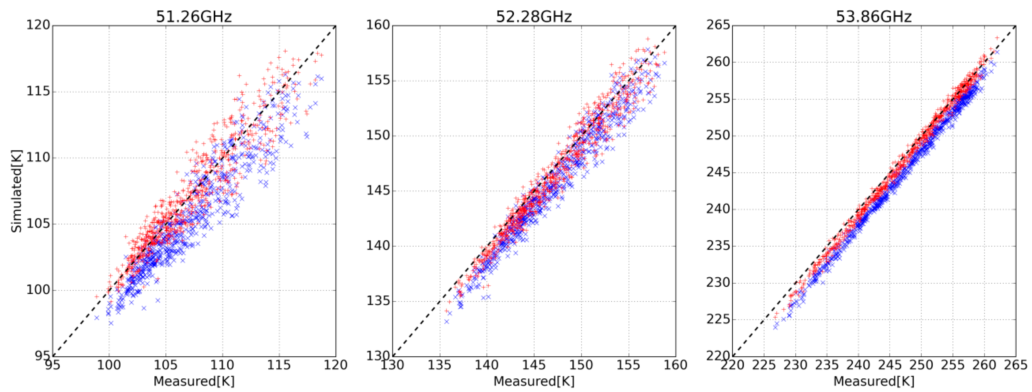
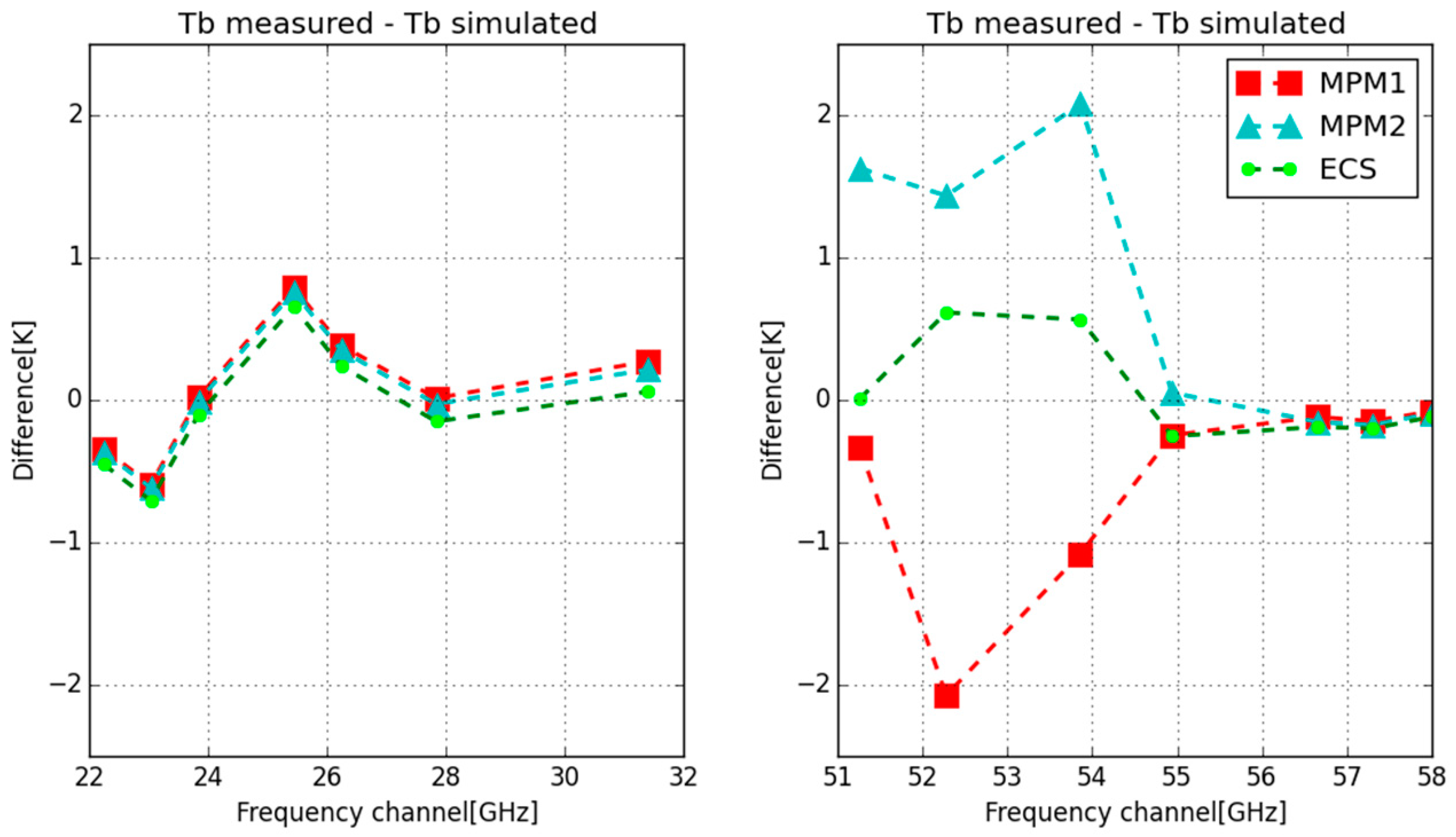
3.1. Results of Simulation

For the simulations of brightness temperature spectra, we used the following atmospheric absorption models:
(1)
MPM1: the MPM, taking into account the first-order mixing [26].
(2)
MPM2: the MPM, taking into consideration the second-order mixing with the coefficients presented in the work [20] and with correction of integral intensity of the band. Note that in [18], this version was called MPM2a.
(3)
ECS: the model including the oxygen band contribution calculated in the ECS approximation and the contribution of other components (in particular, the continuum and the water-vapor absorption spectrum) that are taken from the MPM.
Here, we analyze only zenith (θ = 0) microwave measurements, as it was shown in [18] that in the available setup, we cannot reliably identify the presence of clouds in the scanning regime. Data series for the 51.26, 52.28 and 53.86-GHz channels are presented in Figure 1. The scatter plot in Figure 1 compares the measured brightness temperatures with the simulations that use MPM2 and ECS models. As seen from the figure, the difference between the measured and calculated values is noticeable in all these channels for MPM2 simulations; while most of the points corresponding to the ECS model are closer to the diagonal, which means a better agreement between the calculated and measured brightness temperatures.
The difference between the models is seen especially well in Figure 2, which presents the averaged difference (<ΔTb>) between the measured and calculated brightness temperatures depending on the frequency channel. The <ΔTb> values are ordinary arithmetic means:
Δ T b = k = 1 N T b   m e a s u r e d k T b   m o d e l k N ,
where k is the index in the dataset and N is the total number of cases.
Within the 22–32 GHz frequency range, <ΔTb> is approximately the same and does not exceed 0.8 K for all absorption models. This is due to the fact that, in this range, the water-vapor absorption plays the main role and is the same for the models. For oxygen absorption, the relative difference between the models is small (see Figure 1); in this band, it manifests itself only as a weak, smoothly varying pedestal that includes the wing of the 60-GHz band and non-resonant Debye absorption. Thus, there is almost no difference between the models in the 22–32 GHz band. In the 55–58 GHz frequency range, |<ΔTb>| < 0.2 K for all the models, which is a typical behavior of opaque channels, i.e., the value of (6) is very high at z (see Section 3.2).
The difference between the simulated and measured brightness temperatures is especially pronounced within the 51–54 GHz range that includes the low-frequency wing of the oxygen band. This difference depends significantly on the chosen absorption model. With the use of MPM1 and MPM2, <ΔTb> has the opposite sign and its absolute value amounts to 2 K and more. This value is higher than the typical standard deviation of ΔTb that is almost the same for the models: 0.6 and 1.1 K in the 53.86 and 52.28 GHz channels, respectively. (Note: as standard deviations of ΔTb are almost the same for all the models, Figure 3 in our previous work [18] can illustrate the standard deviations in the current work).
At the same time, the ECS model gives a much better agreement between the measured and calculated brightness temperatures, the maximum mean difference between which does not exceed 0.6 K. It is close to the absolute accuracy of microwave measurements and may be beyond the precision of the comparison procedure (see Section 3.2).

3.2. Accuracy of the Results

As the results presented are to determine what spectroscopic model is closer to the reality, they should undergo meticulous scrutiny. In other words, we need to know to what degree Figure 2 represents the real error in the absorption model. Obviously, we should be skeptical about those features with the amplitude below the absolute accuracy of the measurements (0.5 K). Moreover, the results are subject to distortions: there are inaccuracies in our simulations and there is the influence of the mismatch between the radiosonde profile and the real state of the atmosphere in the line of sight of the device. The latter is hard to characterize in exact terms as it includes the unknown mismatch between the true atmosphere profiles above the IAP RAS measurement facility and the aerological station. In our previous work [18], we conducted an investigation of those distortions. Below, we summarize the results of the investigation and introduce some additional inferences. Note that in this section, only the 50–60 GHz band is considered.
In [18], we made a thorough assessment of the error budget of the brightness temperature simulations (see the related work [35]). The modeling error of using a pencil-beam solution instead of finite antenna-beam simulation is less than 0.015 K for zenith measurements using HATPRO. We also estimated the influence of receiver bandwidth. The calculations show that the discrepancy between the monochromatic simulation and full-bandwidth simulation is 0.15 K (this value corresponds to the worst-case scenario for 52.28 GHz channel, it is several times lower in other channels). The choice of frequencies in the HATRPO design mitigates this error. The accuracy of the Rayleigh–Jeans approximation used in (5) is more than enough in the current band (see [29]). The numerical accuracy of the calculation is excessive (see Section 2). Thus, the inaccuracies in the simulations do not distort the results in Figure 2 by more than 0.16 K (even less for channels other than 52.28 GHz) which is less than absolute accuracy.
There are no exact statements to be made about the influence of the mismatch in atmosphere profiles but there are indications that the corresponding distortion is not major. Using qualitative and quantitative properties of (5) under tropospheric conditions, we can assess the amplitude of distortions with different degrees of certainty, depending on the channel.
The opaque channels, meaning the channels for which τ ( z ) 1 (other arguments in (6) are omitted), do not demonstrate the difference between different absorption models. As was shown in discussion session of [18], the corresponding difference in brightness temperature is proportional to Δα/α2, where Δα is the difference in absorption coefficients. According to the estimates in [18] (see Figure 9 there), the channels 54–60 GHz are opaque in typical tropospheric conditions. Brightness temperature of the opaque channel is close to the average temperature of certain near-surface layer (see Formula (5) in [18] and corresponding explanation). The more opaque the channel is, the thinner the layer. As a result, the mean difference in the opaque channels in Figure 2 indicates the average mismatch in temperature at near-surface levels. It means that, on average, this mismatch does not exceed 0.3 °C (or 0.8 °C in the worst-case scenario, considering the absolute accuracy of microwave measurements). Note that we do not have to factor in the precision of the radiosonde. It is reasonable to assume that objective systematic differences between atmospheric conditions on the radiosonde path and HATPRO’s line of sight is more pronounced at lower levels. Thus, it is unlikely for the mismatch in temperature at any level to significantly exceed 0.8 °C.
The discussed distortions and calibration errors (concerning the absolute accuracy) are certainly not of a noisy nature but neither are they constant in time. The calibration error may shift from calibration to calibration. However, the standard deviation of the investigated difference in Tb is larger than the absolute accuracy; thus, it is hard to investigate the separate shifts. As a result, we cannot make statements about whether averaging has any effect on issues with the absolute error of the measurements. The mismatch in atmosphere profiles surely has a seasonal evolution that is apparent from the consideration of subsets of the database corresponding to the different seasons. For example, the seasonal mean differences in opaque channels are larger (up to several times) than the resulting whole-ensemble means because the winter and summer values compensate for each other. Although the general picture is quite similar for all the seasons, the all-year averaging has apparent benefits.
To assess the properties of (5) under tropospheric conditions quantitatively, we linearize it near the mean atmospheric profile. In order to do that, we parameterize the temperature profile in (5) using the piecewise linear function: T(x,z) where x is the vector of the parameters (values at the knots). The knots coincide with altitude levels used in the representation of HATPRO retrieval results. The latter is done for simplicity because the actual grid is irrelevant in further discussions. As a result, we have a matrix of derivatives K to investigate:
K i j T b ( x , ν i ) x j = T b 0 exp ( τ ( z , ν i ) ) ( z 0 z α i x j d z ) + z 0 z exp ( τ ( z , ν i ) ) ( α i x j T + α i T x j α i T z 0 z α i x j d z ) d z ,
where the corresponding derivatives are
α i x j ( x , z ) α ( T ( x ) , P ( T ( x ) ) , , ν i ) x j = ( α ( , ν i ) T T ( x ) x j + α ( , ν i ) P P ( x ) x j )
The pressure-dependency on x originates from the condition of hydrostatic equilibrium:
P ( x , z ) = P 0 exp ( z 0 z Μ a i r g R   T ( x , z ) d z ) ,
where P0 is the surface air pressure; Μair = 28.9644 g/mol is the average air molar mass; g = 9.8 m/s2 is free fall acceleration; and R is the universal gas constant. Thus, the derivative in (10) is:
P x j ( x , z ) = P ( x , z ) z 0 z Μ a i r g R   T 2 ( x , z ) T ( x , z ) x j d z
In the context of Figure 2, the element of the matrix Kij represents the distortion in the i-th spectral channel due to the temperature mismatch at the j-th altitude level (which we denote as δTbi and δxj, respectively). Although we should consider K for every absorption model separately, in practice, the relative difference in the elements due to the model change is small. Thus, below we represent the analysis of K for the MPM1 model.
Using singular decomposition of K, one can show that some features in Figure 2 cannot be caused by the mismatch in atmosphere profiles as was performed in [18] considering ΔTb for MPM1. The simpler and more descriptive way to analyze K is to look at its elements directly. It was discovered that all elements of a row in K have the same sign: the row for the 51.26 GHz channel consists of negatives while the others consist of positive values. This gives us a simple estimate for the absolute value of the distortion:
| δ T b i | = | j M K i j δ x j | max j | δ x j | | j M K i j | ,
where M = 39 is the total number of levels. The sum across the rows of K is presented in Table 1.
Note that the values for opaque channels in Table 1 are close to one. That is expected as brightness temperature in those channels should follow the average temperature in the near-surface layer. The row sums for 51.26 and 52.28 GHz channels are −0.073 and 0.21, respectively. Thus, for the distortion in those channels to exceed the absolute accuracy, the mismatch should reach up to 2.38 °C. This value, though not impossible, is still higher than the 0.8 °C estimated for lower levels. The same estimate for 53.86 GHz yields 0.57 °C, which is possible according to our assumptions. It means that the distortion in this channel may be significant enough.
Considering the estimates of the simulation accuracy and possible distortions of the brightness temperature calculation, we conclude the following: All the simulations are indistinguishably close to the measurements in the 54–60 GHz band as mean differences at those channels do not exceed absolute accuracy of the measurements. This means that although there is a difference between the models in the 54.94 GHz channel, we cannot state which is in better agreement with the measurements. In the 51.26 GHz channel, MPM1 and ECS are indistinguishably close to the measurements while MPM2 results differ significantly. In the 52.28 and 53.86 GHz channels, simulations using the ECS model are in good agreement with the measurements while use of other models leads to a significant difference. It should be noted that, although the 53.86 GHz channel is subject to possible distortion, the results of other models are so far off that, even considering the distortion, the ECS model is more likely to be close to the measurements.

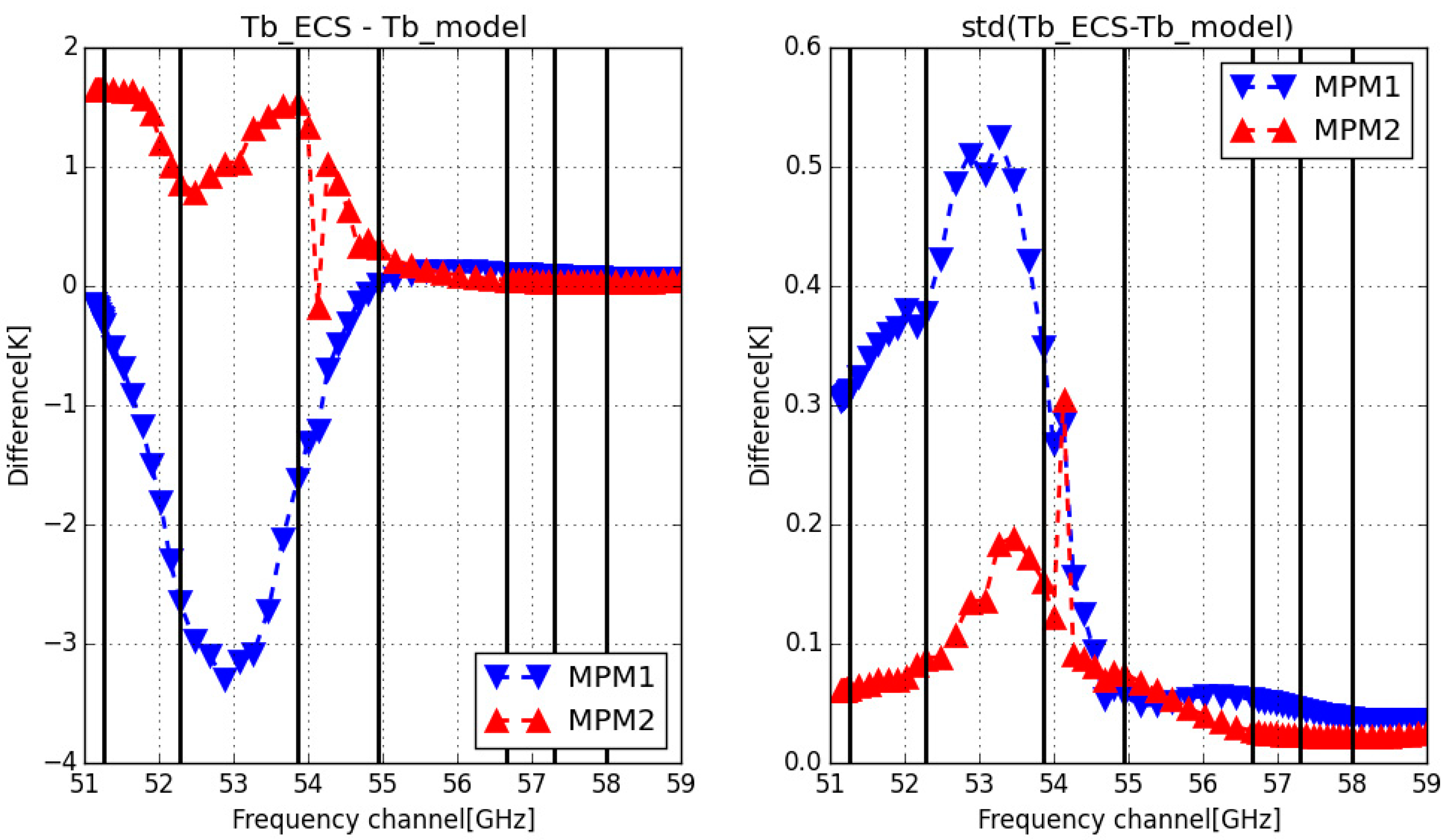
3.3. Spectral Difference with High Spectral Resolution

The discussion above allows us to conclude that the observed systematic difference between the calculated and measured brightness temperatures on the slope of the oxygen band is likely to be of a spectroscopic nature, i.e., there is a systematic difference between the real atmospheric absorption and the modeled one. The difference with a higher (than the one shown in Figure 2) spectral resolution of the brightness temperature calculated by Equation (5) is presented in Figure 3, where the mean difference is shown on the left panel and the standard deviation on the right panel. Due to the lack of measurements with high spectral resolution, Figure 3 shows the differences between the calculated spectra of the models, namely the difference between ECS and MPM1 (Tb_ECSTb_MPM1) and ECS and MPM2 (Tb_ECSTb_MPM2). It is noteworthy that the standard deviation is an order of magnitude smaller than the average difference between the models. Therefore, the change of the model in the retrieval manifests itself as a systematic difference. As seen from this figure, the maximum difference between the model spectra is observed in the 51–53 GHz frequency range, and is about 3.2 K for Tb_ECS−Tb_MPM1 and about 1.7 K for Tb_ECSTb_MPM2. Such a difference, approximately an order of magnitude higher than the accuracy of the present-day spectroradiometers, points to a significant impact of the choice of absorption model when working with radiometric data. There is a seeming outlier (near the 54 GHz frequency) in the values presented in Figure 3, which is especially prominent in Tb_ECSTb_MPM2 values. In fact, it represents the valid calculations when the frequency is close to the center of the narrow line corresponding to the stratospheric oxygen absorption.
Figure 3. Difference between brightness temperature spectra calculated using ECS model, MPM1, and MPM2. Calculations were made by averaging over the ensemble of radiosonde temperature profiles. Mean difference is shown on the left panel, standard deviation is shown on the right panel. Vertical lines indicate the location of the RPG-HATPRO radiometer channels.
Remotesensing 14 06042 g003

4. Conclusions

In summary, the use of the ECS model in simulations yields a much better agreement between the measured and calculated brightness temperatures than the use of the MPM model, which is widely utilized in remote-sensing applications. The superior ECS performance is consistent with its better agreement with laboratory spectroscopic data. We believe that the use of the ECS model in temperature-profile retrieval from radiometric measurements will improve the retrieval accuracy in lower-atmosphere microwave soundings; this, in turn, will improve the quality of weather and hazardous meteorological phenomena forecasting based on these data.
The work presented here utilizes the dataset of only one measurement site. The reproduction of the study in a wider range of atmospheric conditions using multiple independent devices will benefit the scientific community greatly. We encourage other research groups to follow our steps. The latest version of MPM1 model is available at [26]; please refer to [14] as on overview of the model. MPM2 is described in [20]. To learn more about the ECS model, please refer to [19] and references therein, while the works of [27], [28] and [23] provide historical background. To obtain MPM2 and ECS models, please refer to the data availability section below.

Author Contributions

Conceptualization, M.Y.K. and A.M.F.; methodology, M.Y.K., M.V.B. and A.M.F.; software, M.V.B. and D.S.M.; validation, M.V.B. and D.S.M.; formal analysis, M.V.B. and D.S.M.; investigation, M.V.B., D.S.M. and E.A.S.; resources, M.V.B.; data curation, M.V.B. and D.S.M.; writing—original draft preparation, E.A.S. and M.V.B.; writing—review and editing, E.A.S. and M.V.B.; visualization, E.A.S. and M.V.B.; supervision, E.A.S. and M.Y.K.; project administration, E.A.S. and M.Y.K.; funding acquisition, E.A.S. All authors have read and agreed to the published version of the manuscript.

Funding

This work was supported by the Russian Science Foundation under grant No. 18-72-10113, https://rscf.ru/en/project/18-72-10113/, accessed on 24 November 2022. Microwave data were obtained within the framework of the Russian State project No 0030-2021-0008.

Data Availability Statement

Data presented in this study are available on request from the corresponding author. The MPM2 model is available on request from D.S. Makarov ([email protected]). The ECS model is available on the website of the Microwave Spectroscopy laboratory of IAP RAS: https://mwl.ipfran.ru/#/instrum, accessed on 24 November 2022.

Acknowledgments

The authors would like to thank Mikhail Yu. Tretyakov for his advice and assistance.

Conflicts of Interest

The authors declare no conflict of interest. The funders had no role in the design of the study; in the collection, analyses, or interpretation of data; in the writing of the manuscript; or in the decision to publish the results.

References

  1. Chan, P.W. Performance and application of a multiwavelength, ground-based microwave radiometer in intense convective weather. Meteorol. Z. 2009, 18, 253–265. [Google Scholar] [CrossRef]
  2. Chan, P.W.; Hon, K.K. Application of ground-based, multichannel microwave radiometer in the nowcasting of intense convective weather through instability indices of the atmosphere. Meteorol. Z. 2011, 20, 431–440. [Google Scholar] [CrossRef]
  3. Madhulatha, A.; Rajeevan, M.; Venkat Ratnam, M.; Bhate, J.; Naidu, C.V. Nowcasting severe convective activity over southeast India using ground-based microwave radiometer observations. J. Geophys. Res. Atmos. 2013, 118, 1–13. [Google Scholar] [CrossRef] [Green Version]
  4. Venkat Ratnam, M.; Durga Santhi, Y.; Rajeevan, M.; Vijaya Bhaskara Rao, S. Diurnal variability of stability indices observed using radiosonde observations over a tropical station: Comparison with microwave radiometer measurements. Atmos. Res. 2013, 124, 21–33. [Google Scholar] [CrossRef]
  5. Cimini, D.; Rizi, V.; Di Girolamo, P.; Marzano, F.S.; Macke, A.; Pappalardo, G.; Richter, A. Overview: Tropospheric profiling: State of the art and future challenges—Introduction to the AMT special issue. Atmos. Meas. Technol. 2014, 7, 2981–2986. [Google Scholar] [CrossRef]
  6. Cimini, D.; Nelson, M.; Güldner, J.; Ware, R. Forecast indices from a ground-based microwave radiometer for operational meteorology. Atmos. Meas. Technol. 2015, 8, 315–333. [Google Scholar] [CrossRef] [Green Version]
  7. Kulikov, M.Y.; Belikovich, M.V.; Skalyga, N.K.; Shatalina, M.V.; Dementyeva, S.O.; Ryskin, V.G.; Shvetsov, A.A.; Krasil’nikov, A.A.; Serov, E.A.; Feigin, A.M. Skills of Thunderstorm Prediction by Convective Indices over a Metropolitan Area: Comparison of Microwave and Radiosonde Data. Remote Sens. 2020, 12, 604. [Google Scholar] [CrossRef] [Green Version]
  8. Isaac, G.A.; Bailey, M.; Boudala, F.S.; Burrows, W.R.; Cober, S.G.; Crawford, R.W.; Donaldson, N.; Gultepe, I.; Hansen, B.; Heckman, I.; et al. The Canadian Airport Nowcasting System (CAN-Now). Meteorol. Appl. 2014, 21, 30–49. [Google Scholar] [CrossRef]
  9. Güldner, J. A model-based approach to adjust microwave observations for operational applications: Results of a campaign at Munich Airport in winter 2011/2012. Atmos. Meas. Technol. 2013, 6, 2879–2891. [Google Scholar] [CrossRef] [Green Version]
  10. Ware, R.; Cimini, D.; Campos, E.; Giuliani, G.; Albers, S.; Nelson, M.; Koch, S.E.; Joe, P.; Cober, S. Thermodynamic and liquid profiling during the 2010 Winter Olympics. Atmos. Res. 2013, 132–133, 278–290. [Google Scholar] [CrossRef]
  11. Rosenkranz, P.W. Shape of the 5 mm oxygen band in the atmosphere. IEEE Trans. Antennas Propagat. 1975, 23, 498–506. [Google Scholar] [CrossRef]
  12. Liebe, H.; Grimmestad, G.; Hopponen, J. Atmospheric oxygen microwave spectrum—Experiment versus theory. IEEE Trans. Antennas Propagat. 1977, 25, 327–335. [Google Scholar] [CrossRef]
  13. Liebe, H.J.; Rosenkranz, P.W.; Hufford, G.A. Atmospheric 60-GHz oxygen spectrum: New laboratory measurements and line parameters. J. Quant. Spectrosc. Radiat. Transfer. 1992, 48, 629–643. [Google Scholar] [CrossRef]
  14. Liebe, H.J. MPM—An atmospheric millimeter-wave propagation model. Int. J. Infrared Millim. Waves 1989, 10, 631–650. [Google Scholar] [CrossRef]
  15. Tretyakov, M.Y.; Koshelev, M.A.; Dorovskikh, V.V.; Makarov, D.S.; Rosenkranz, P.W. 60-GHz Oxygen Band: Precise broadening and central frequencies of fine-structure lines, absolute absorption profile at atmospheric pressure, and revision of mixing coefficients. J. Mol. Spectrosc. 2005, 231, 1–14. [Google Scholar] [CrossRef]
  16. Cimini, D.; Rosenkranz, P.W.; Tretyakov, M.Y.; Koshelev, M.A.; Romano, F. Uncertainty of atmospheric microwave absorption model: Impact on ground-based radiometer simulations and retrieval. Atmos. Chem. Phys. 2018, 18, 15231–15259. [Google Scholar] [CrossRef] [Green Version]
  17. Wentz, F.J.; Meissner, T. Atmospheric absorptionmodel for dry air and watervapor at microwave frequencies below 100GHz derived from spaceborne radiometer observations. Radio Sci. 2018, 51, 381–391. [Google Scholar] [CrossRef] [Green Version]
  18. Belikovich, M.V.; Kulikov, M.Y.; Makarov, D.S.; Skalyga, N.K.; Ryskin, V.G.; Shvetsov, A.A.; Krasil’nikov, A.A.; Dementyeva, S.O.; Serov, E.A.; Feigin, A.M. Long-term observations of microwave brightness temperatures over a metropolitan area: Comparison of radiometric data and spectra simulated with the use of radiosonde measurements. Remote Sens. 2021, 13, 2061. [Google Scholar] [CrossRef]
  19. Makarov, D.S.; Tretyakov, M.Y.; Boulet, C. Line Mixing in the 60-GHz Atmospheric Oxygen Band: Comparison of the MPM and ECS Model. J. Quant. Spectrosc. Radiat. Transf. 2013, 124, 1–10. [Google Scholar] [CrossRef]
  20. Makarov, D.S.; Tretyakov, M.Y.; Rosenkranz, P.W. Revision of the 60-GHz atmospheric oxygen absorption band models for practical use. J. Quant. Spectrosc. Radiat. Transfer. 2020, 243, 106798. [Google Scholar] [CrossRef]
  21. Gordon, R.G. Semiclassical theory of spectra and relaxation in molecular gases. J. Chem. Phys. 1966, 45, 1649–1655. [Google Scholar] [CrossRef]
  22. Lam, K.S. Application of pressure broadening theory to the calculation of atmospheric oxygen and water vapor microwave absorption. J. Quant. Spectrosc. Radiat. Transfer. 1977, 17, 351–383. [Google Scholar] [CrossRef]
  23. Tran, H.; Boulet, C.; Hartmann, J.-M. Line mixing and collision-induced absorption by oxygen in the A-band: Laboratory measurements, model, and tools for atmospheric spectra computations. J. Geophys. Res. 2006, 111, D15210. [Google Scholar] [CrossRef] [Green Version]
  24. Twomey, S. On the numerical solution of Fredholm integral equations of the first kind by the inversion of the linear system produced by quadrature. J. Assoc. Comput. Mach. 1963, 10, 97–101. [Google Scholar] [CrossRef]
  25. Koshelev, M.A.; Vilkov, I.N.; Tretyakov, M.Y. Collisional broadening of oxygen fine structure lines: The impact of temperature. J. Quant. Spectrosc. Rad. Transf. 2016, 169, 91–95. [Google Scholar] [CrossRef]
  26. Rosenkranz, P.W. Line-by-Line Microwave Radiative Transfer (Non-Scattering). Remote Sens. Code Library. Available online: http://cetemps.aquila.infn.it/mwrnet/lblmrt_ns.html (accessed on 15 August 2022).
  27. DePristo, A.E.; Augustin, S.D.; Ramaswamy, R.; Rabitz, H. Quantum number and energy scaling for nonreactive collisions. J. Chem. Phys. 1979, 71, 850–865. [Google Scholar] [CrossRef]
  28. Niro, F.; Boulet, C.; Hartmann, J.-M. Spectra calculations in central and wing region of CO2 IR bands between 10 and 20 μm. I: Model and laboratory measurements. J. Quant. Spectrosc. Radiat. Transf. 2004, 88, 483–498. [Google Scholar] [CrossRef]
  29. Rosenkranz, P.W. Absorption of microwaves by atmospheric gases. In Atmospheric Remote Sensing by Microwave Radiometry; Janssen, M.A., Ed.; John Wiley & Sons: New York, NY, USA, 1993; pp. 37–90. [Google Scholar]
  30. Instrument Operation and Software Guide. Available online: http://www.radiometer-physics.de/download/PDF/Radiometers/HATPRO/RPG_MWR_STD_Software_Manual%20G5.pdf (accessed on 15 August 2022).
  31. Technical Instrument Manual. Available online: http://www.radiometer-physics.de//downloadftp/pub/PDF/Radiometers/General_documents/Manuals/2015/RPG_MWR_STD_Technical_Manual_2015.pdf (accessed on 15 August 2022).
  32. LLC “AEROPRIBOR”. Available online: http://zondr.ru/development-product/10-ak-2.html (accessed on 15 August 2022).
  33. Picone, J.M.; Hedin, A.E.; Drob, D.P.; Aikin, A.C. NRLMSISE-00 empirical model of the atmosphere: Statistical comparisons and scientific issues. J. Geophys. Res. 2002, 107, 1468. [Google Scholar] [CrossRef]
  34. De Angelis, F.; Cimini, D.; Löhnert, U.; Caumont, O.; Haefele, A.; Pospichal, B.; Martinet, P.; Navas-Guzmán, F.; Klein-Baltink, H.; Dupont, J.-C.; et al. Long-term observations minus background monitoring of ground-based brightness temperatures from a microwave radiometer network. Atmos. Meas. Technol. 2017, 10, 3947–3961. [Google Scholar] [CrossRef] [Green Version]
  35. Meunier, V.; Löhnert, U.; Kollias, P.; Crewell, D. Biases cause by the instrument bandwidth and beam width on simulated brightness temperature measurements from scanning microwave radiometers. Atmos. Meas Technol. 2013, 6, 1171–1187. [Google Scholar] [CrossRef]
Figure 1. The set of points corresponding to comparison of the measured and calculated brightness temperatures under the same conditions in three frequency channels: 51.26, 52.28 and 53.86 GHz. All the points were obtained in clear-sky conditions. Red crosses—ECS model; blue crosses—MPM2. Note that Figure 1 in [18] depicts a similar plot for MPM1 and MPM2 models.
Remotesensing 14 06042 g001
Figure 2. Ensemble-averaged difference between the measured and calculated brightness temperatures at the frequencies of the RPG-HATPRO radiometer channels. Symbols of different color and shape correspond to calculations using different absorption models.
Remotesensing 14 06042 g002
Table 1. Row sums of K.
Channel (GHz)51.26 52.28 53.86 54.9456.6657.3 58
Row   sum   j = 1 M K i j [K/°C]−0.0730.210.870.960.980.980.98
Publisher’s Note: MDPI stays neutral with regard to jurisdictional claims in published maps and institutional affiliations.

