AQE-Net: A Deep Learning Model for Estimating Air Quality of Karachi City from Mobile Images

Abstract

Air quality has a significant influence on the environment and health. Instruments that efficiently and inexpensively detect air quality could be extremely valuable in detecting air quality indices. This study presents a robust deep learning model named AQE-Net, for estimating air quality from mobile images. The algorithm extracts features and patterns from scene photographs collected by the camera device and then classifies the images according to air quality index (AQI) levels. Additionally, an air quality dataset (KARACHI-AQI) of high-quality outdoor images was constructed to enable the model’s training and assessment of performance. The sample data were collected from an air quality monitoring station in Karachi City, Pakistan, comprising 1001 hourly datasets, including photographs, PM2.5 levels, and the AQI. This study compares and examines traditional machine learning algorithms, e.g., a support vector machine (SVM), and deep learning models, such as VGG16, InceptionV3, and AQE-Net on the KHI-AQI dataset. The experimental findings demonstrate that, compared to other models, AQE-Net achieved more accurate categorization findings for air quality. AQE-Net achieved 70.1% accuracy, while SVM, VGG16, and InceptionV3 achieved 56.2% and 59.2% accuracy, respectively. In addition, MSE, MAE, and MAPE values were calculated for our model (1.278, 0.542, 0.310), which indicates the remarkable efficacy of our approach. The suggested method shows promise as a fast and accurate way to estimate and classify pollutants from only captured photographs. This flexible and scalable method of assessment has the potential to fill in significant gaps in the air quality data gathered from costly devices around the world.

1. Introduction

Air pollution has worsened over the past few decades; therefore, it has received significant attention from scholars and policymakers. 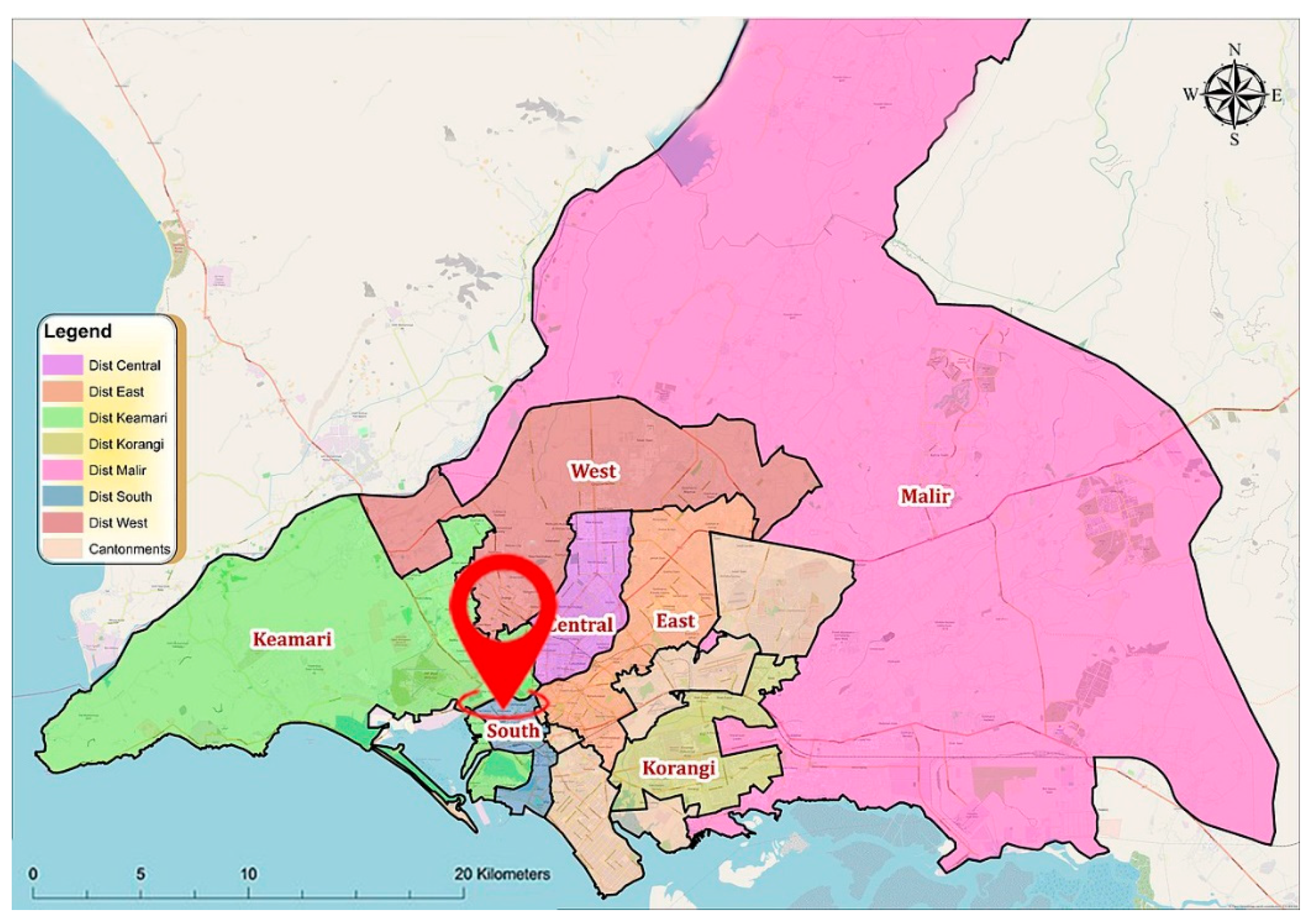An air quality index (AQI), which is composed of six pollutants, including particulate matter 10 (PM₁₀), particulate matter 2.5 (PM_2.5), sulfur dioxide (SO₂), nitrogen dioxide (NO₂), carbon monoxide (CO), and ozone (O₃), is an overall index that can more objectively depict the levels of air pollution than an index that includes a single air contaminant [1,2]. Pakistan has invariably encountered severe air pollution issues caused by industrial sources and automobile exhausts, particularly in Karachi City, located in southern Pakistan [3]. Consequently, air pollution poses a severe threat to health, and prompt monitoring of air quality is vital to control pollution and immensely useful for protecting human health. Air pollution has a variety of adverse effects, both physiological and psychological, on people’s health. It is a contributor to the development of infectious illnesses. In 2012, infectious diseases were responsible for the deaths of 9,500,000 people all over the world. Air pollution is a clear warning sign of potential danger to one’s health [4]. Additionally, when breathing polluted air, people should consider the possibility that they could catch an illness. Long-term exposure to extremely high PM2.5 concentrations has been linked to the onset of cardiovascular disease and other major health problems, as well as negative effects on the liver and lungs [5,6,7].

Currently, air quality data collection is mostly micro-station based. Though, because of the expensive material and set-up costs of advanced sensors, such in-situ monitoring is less possible in the majority of regions of concern, and this represents a significant financial burden for developing and emerging nations in the long term [8]. It is possible to use image-based systems for air quality monitoring as a backup when gauges are unavailable or when they are not operating effectively. Recently, there have been several initiatives to build low-cost air pollution monitoring equipment [9,10,11,12]. Predictions of air pollution are primarily based on deterministic [13,14,15,16,17] and statistical models. The deterministic approach makes use of a theoretical meteorological emission and a chemical model to simulate the creation and diffusion process of contaminants. However, because of the ideal theory used to determine the model structure and estimate parameters, it falls short of explaining the nonlinearity and heterogeneity of many factors connected to pollution generation. When compared to the deterministic approach, the statistical method’s use of a data-driven statistical modeling strategy allows it to sidestep the complexity and hassle of modeling while still delivering impressive results.

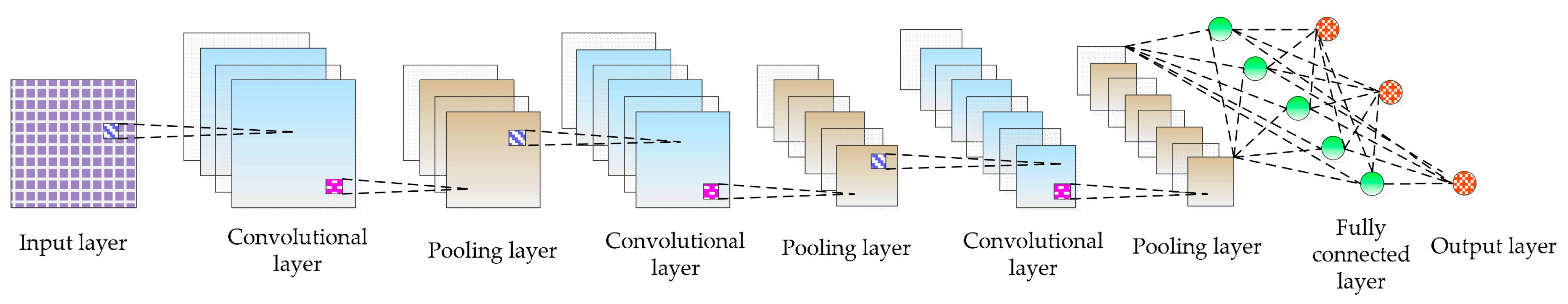
Machine learning (ML) has recently achieved substantial advancements in numerous areas, including speech and image recognition, with improved eminent excellence. The convolutional neural network, abbreviated as CNN, has seen extensive use in research in the fields of computer vision and image processing, with credible performance in attempting various inspiring tasks on classification and estimation [18,19,20,21,22,23,24,25,26]. The use of machine learning and deep learning methods in analyzing air quality has grown in popularity in recent years [27,28,29]. Air pollution has been classified or estimated using image processing in many studies [12,30,31,32]. Additionally, an image-based air pollution estimate provides a promising future; however, few such studies have been conducted in this context. Therefore, more investigation into image-based air quality estimates is needed to boost accuracy and reliability. Due to the rapid growth of machine learning algorithms and computer vision technology, recently, many automatic algorithms have been offered as potent tools to address the crack detection difficulties in practice [33]. With the use of deep convolutional neural networks (DCNNs) and an improved chicken swarm algorithm, the authors of [34] created a visual method for diagnosing cracks (ECSA). To better forecast and analyze the air pollution generated by Combined Cycle Power Plants, a novel hybrid intelligence model based on long short-term memory (LSTM) and multi-verse optimization algorithm (MVO) has been created [35,36]. This developed a deep learning model to predict PM2.5 atmospheric air pollution using meteorological data, ground-based observations, and big data from remote-sensing satellites. To forecast the concentration of air pollutants in various areas inside a city, using spatial-temporal correlations, a convolutional neural network with a long short-term memory deep neural network (CNN-LSTM) model was developed [37]. Using a recurrent neural network deep learning model, the presence of SO2 and PM10 in the air of Sakarya city was demonstrated [38]. In order to forecast the quality of the air, [39] a spatio-temporal deep learning model called Conv1D-LSTM, which integrates a deep convolutional neural network (1D CNN) with a long short-term memory (LSTM) to extract spatial and temporal correlation data, was presented [40]. The model presented the application of an attention-based convolutional BiLSTM autoencoder model for air quality forecasting.

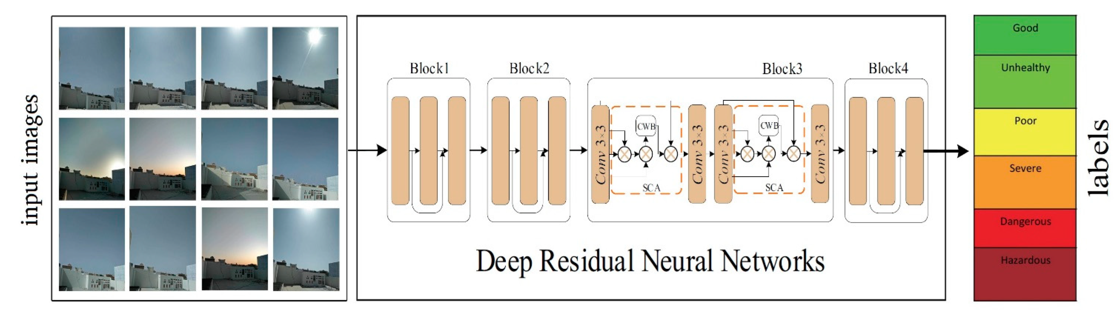
This study proposes a deep CNN model (AQE-Net) based on ResNet to classify photos per air quality level. Previous approaches based on CNN networks concentrate almost solely on PM2.5, despite the fact that PM2.5 is just a small component of air pollution and does not accurately reflect overall air quality information. Additionally, the existing studies have estimated air quality in different aspects. Among them, much research focuses on particular pollutants. However, this study contributes theoretically and practically and takes AQI as an outcome variable to estimate air quality. Moreover, many studies use satellite images for air quality estimations. In contrast, this study uses mobile images. Therefore, more investigations into image-based air quality estimates are needed to boost accuracy and reliability. Our proposed model can measure the AQI directly, more accurately estimating the environment’s air quality. In this context, this study investigates the connection between air quality and image characteristics using air quality analysis of many fixed-site photographs, builds a prediction model, and calculates air quality everywhere. People can collect pictures easily and quickly using portable terminals such as mobile phones, tablets, and other smart devices and can use this method to estimate the AQI in real-time.

2. Materials and Methods

2.1. Study Area

This study focuses on Pakistan’s largest metropolitan city, Karachi, the capital of the Sindh province. It is the twelfth-largest city in the world, with a population of over 12 million people. Karachi comprises seven districts: the Karachi Central, Karachi East, Karachi South, Karachi West, Korangi, Malir, and Keamari districts. Additionally, Clifton is part of the Karachi South district, which is our main research area for this study. Figure 1 shows the Karachi map with all districts, and the location symbol indicates the Clifton area on the map.

2.2. Dataset

Due to the lack of a publicly available image library for air quality related to image detection, the KHI-AQI image database was created. There are a total of 1001 photographs in the library, which are a series of scene images captured at varying levels of air quality. To create the dataset, we went through the following stages.

We installed a mobile device with a camera in a firm position and orientation nearby the US Consulate General’s monitoring station in Karachi to capture surrounding air quality images. Every hour from 8:00 am to 18:00 pm, the camera collects photographs of the sky that are automatically saved. The information about the air quality image collecting points is included in

Table 1. Information about the image acquisition process.

Collection Point	Clifton Store Karachi
Photo pixels (Px)	1706 × 1280
Shooting time period	8:00–18:00
Collection interval	Hourly
Camera equipment	OppoA37 (Mobile)
Total period	3 months (Aug 2021 to Oct 2021)

. Further, Figure 2 depicts an example of scene images from the air quality image library that correspond to different degrees of air pollution levels. In Figure 2, Pictures (a), (b), (c), (d) and (e) were taken at 8:00, 9:00, 10:00, 11:00, and 12:00, respectively, while pictures (f), (g), (h), (i) and (j) were obtained at 13:00, 14:00, 15:00, 16:00, and 17:00.

We accessed monitoring station data from the MicroStation for air quality at the United States embassies and consulates in Karachi from 1^st August, 2021 to 30^th October, 2021, a total of three months of data [41]. Figure 3 shows the AQI data points for these three months. The hourly data were then translated to levels in accordance with the AQI classification table, which indicates the concentration of AQI in the atmosphere. We noted the file name and capturing time of the photographs captured at each collecting point. They comprised the following fields: AQI value, image name, AQI level, capturing time, and others. There has been an overall collection of 1001 data points, with the level of AQI serving as the picture label. As a result, image collection and observation data related to the geographic place and time have been gathered, and the database has been produced with higher quality site and air quality images (

Table 2. Information about the dataset of samples.

Capturing Time	Image Name	Air Time	AQI	Classes
2021/1/6 8:00:00	DSCF0667.JPG	2021/1/6 8:00:00	114	3
2021/1/6 8:00:00	DSCF0667.JPG	2021/1/6 8:00:00	123	3
2021/1/6 8:00:00	DSCF0667.JPG	2021/1/6 8:00:00	90	2
2021/1/6 8:00:00	DSCF0667.JPG	2021/1/6 8:00:00	87	2

).

2.3. Convolutional Neural Network (CNN)

Fukushima and Miyake (1982) [42] proposed a convolutional neural network (CNN) in 1980, which was then updated by LeCun et al. (1989) [43]. A number of areas in which CNN has succeeded in recent years include synthetic biomedicine [44], catastrophe detection [45], natural language processing [46], holographic image reconstruction [47], the artificial intelligence program of Go [48], optical fiber communication [49], and so on. Using high-performance computing platforms like high-performance computers, graphics workstations, cloud computing platforms, etc., it is now possible to train complicated models using large-scale datasets. There have been a wide array of convolution neural network models developed in this regard, including ZFNet [50], GoogleNet [51], LeNet [52], MobileNets [53], VGGNet [54], Overfeat model [55], DenseNet [56], SPPNet [57], ResNet [58], AlexNet [59], and so on. A CNN is a multilayer network with a fundamental structure that is mostly composed of the following layers: the input layer, the convolutional layer, the pooling layer, the completely connected layer, and the output layer, as illustrated in Figure 4.

2.4. AQE-NET Model

The training set for the model is defined as ${\left\{\left({\mathrm{x}}_{\mathrm{i}},{\mathrm{y}}_{\mathrm{i}}\right)\right\}}_{\mathrm{i}=1}^{\mathrm{N}},{ \mathrm{x}}_{\mathrm{i}}\in {ℝ}^{\mathrm{H}\times \mathrm{E}\times \mathrm{C}},{\mathrm{y}}_{\mathrm{i}}\in \mathrm{N}$. A collection of air quality evaluation images and a set of labels are referred to as ${\left\{{\mathrm{x}}_{\mathrm{i}}\right\}}_{\mathrm{i}=1}^{\mathrm{N}}$, and ${\left\{{\mathrm{y}}_{\mathrm{i}}\right\}}_{\mathrm{i}=1}^{\mathrm{N}}$, respectively. When an image ${\mathrm{x}}_{\mathrm{i}}$ is input, it is needed to acquire the air quality level ${\mathrm{y}}_{\mathrm{i}}$ that corresponds to the image ${\mathrm{x}}_{\mathrm{i}}$, as well as the mapping relationship ${\mathrm{y}}_{\mathrm{i}}=\mathrm{F}\left({\mathrm{x}}_{\mathrm{i}}\right)$. Figure 5 depicts the overall structure of our model.

The AQE-Net is built from merging a self-supervision module known as the Spatial and Context Attention block with a network of other self-supervision modules (SCA); it was previously built in conjunction with the original ResNet18 [58] network structure to design a feature extraction network for air quality pictures. The residual unit is the unit that is most susceptible to changes in weight. The self-monitoring module can continually adjust the relevance of feature information, allowing the model to come closer to the overall best solution. The third module was expanded to include a module for scene self-supervision, although the original structure was unchanged. The third block consists of two residual structures. Each residual structure has an SCA module, and the feature map from the input SCA module is utilized in the third module, which has a resolution of 1/16 of the initial input image, resulting in a considerable reduction in the amount of computation required for matrix multiplication. After three branches, the feature map generates various pieces of contextual scene feature information. The first branch determines the correlation amongst each pixel from the air quality image and then matrix-multiplies the 1st branch’s output by the 2nd branch’s output to obtain the similarity between distinct channel maps. The third branch forms feature maps by matrix multiplication with the result to disperse relevant feature properties back to the original initial feature map to identify the relationship between the complete feature map information. The feature map is then combined by utilizing global average pooling [52] and multiplied with the input feature map to get the final output. A recent study [60,61] demonstrated that self-supervised learning could significantly increase network performance. Figure 6 shows how the SCA block unit is integrated into the network architecture. Using rich relevant information, the SCA module re-calibrates the feature mapping throughout channels while concurrently emphasizing key feature information and hiding information that is not connected to the feature mapping. The primary structure of the SCA is divided into two components. Part one encodes the overall scene context into local characteristics, examines the similarity across channels, and increases the representational capacities of the scene. For each channel, the second component integrates spatial context information to strengthen and accurately manage the dependence between the scenes.

Firstly, the input feature graph $\mathrm{X}\in {ℝ}^{\mathrm{H}\times \mathrm{W}\times \mathrm{C}}$ is created first using $\mathsf{\Phi }(·)$ and $\mathsf{\Psi }(·)$ operations to form a new feature graph of $\mathrm{A}\in {ℝ}^{\mathrm{H}\times \mathrm{W}\times {\mathrm{C}}_1}$ and $\mathrm{B}\in {ℝ}^{\mathrm{H}\times \mathrm{W}\times {\mathrm{C}}_1}$, as seen in Figure 2. The $\mathsf{\Phi }(·)$ and $\mathsf{\Psi }(·)$ operations indicate convolutional layers containing batch normalization [62] and ReLu layers [63]. The size of the convolution kernel can be adjusted to $\left[1\times 1\times {\mathrm{C}}_1\right]$ in order to limit the amount of calculation required. Where ${\mathrm{C}}_1=\frac{1}{16}\mathrm{C}$, the dimension of channel can be lowered, as well as reducing the number of matrix multiplication calculations required. The feature map $\mathrm{A}$ to ${ℝ}^{{\mathrm{C}}_1\times \mathrm{HW}}$ is resized and then transposed to ${ℝ}^{\mathrm{HW}\times {\mathrm{C}}_1}$ when the $\mathrm{Z}$ reshape is complete. Finally, multiply $\mathrm{A}$ and $\mathrm{B}$ in matrix fashion and apply the softmax function to produce a map of $\mathrm{Z}\in {ℝ}^{{\mathrm{C}}_1\times {\mathrm{C}}_1}$ of the channel’s correlation. The equation is given below:

$$Z_{ij}=\frac{\left(\mathsf{\psi }{\left(X_i\right)}^T·\mathsf{\varphi }\left(X_j\right)\right)}{{{\displaystyle \sum }}_{j=1}^{HW}exp\left(\left(\mathsf{\psi }\left(X_i\right)·\mathsf{\varphi }\left(X_j\right)\right)\right)}$$

(1)

In this case, $X_i$ denotes the number $\mathrm{i}$ indexed pixel from the feature vector. $\mathrm{j}$ denotes the index for total possible locations. The relationship between each remaining pixel and $\mathrm{i}$ is represented by the letter ${\mathrm{Z}}_{\mathrm{ij}}$. Simultaneously, once the feature map $\mathrm{X}$ is given as input to $\mathsf{{\rm K}}(·)$, the feature map $\mathrm{E}\in {ℝ}^{\mathrm{H}\times \mathrm{W}\times {\mathrm{C}}_1}$ is formed, and then feature map $\mathrm{E}$ is transposed to ${ℝ}^{{\mathrm{C}}_1\times \mathrm{HW}}$ after being reshaped. $\mathsf{{\rm K}}(·)$ has the same function as $\mathsf{\Phi }(·)$ and $\mathsf{\Psi }(·)$. In order to redistribute the correlation information to the original feature map, it is matrix-multiplied to feature map $\mathrm{Z}$. The feature map $\mathrm{D}\in {ℝ}^{\mathrm{H}\times \mathrm{W}\times {\mathrm{C}}_1}$ is then obtained by reshaping the acquired result into ${ℝ}^{\mathrm{H}\times \mathrm{W}\times {\mathrm{C}}_1}$. Given below is the calculation equation.

$$D_{j=}{{\displaystyle \sum }}_{j=1}^{HW}{Z}_{ij}\mathsf{{\rm K}}\left(X_i\right)$$

(2)

The spatial attention mechanism is used to aggregate the scene context mapping in order to create the feature map $\mathrm{D}$, and the connected channels benefit from each other (Equation (2)). In order to appropriately optimize the correlation between every channel in the feature map $\mathrm{X}$ and other channels, the channel of the feature map $\mathrm{D}$ is weighted by applying the channel-wise module. First, a channel-wise statistic $\mathrm{V}\in {ℝ}^{{\mathrm{C}}_1}$ is calculated using the global average pooling to aggregate the spatial dimension $\mathrm{W}\times \mathrm{H}$ of the feature map $\mathrm{D}$, where the number $\mathrm{i}$ item in $\mathrm{V}$ is determined as follows:

$$V_i=\frac{1}{W\times H}{{\displaystyle \sum }}_{n=1}^W{{\displaystyle \sum }}_{m=1}^H{D}_i\left(n,m\right)$$

(3)

The feature map $\mathrm{X}$ includes $\mathrm{C}$ channels. To alter the dimension from $\mathrm{w}$ to ${ℝ}^{\mathrm{C}}$, a new, fully connected layer is added. The method for calculation is as follows:

$$Z=F\left(v,W\right)=\sigma \left(Wv\right)$$

(4)

where the Sigmoid activation function $\mathrm{W}\in {ℝ}^{{\mathrm{C}}_1\times \mathrm{c}}$ is represented by $\mathsf{\sigma }$. Finally, the SCA module’s final output complies with the updated feature map G:

$$g_i=F_{scale}\left(X_i,Z_i\right)=X_i·Z_i$$

(5)

where the feature map $\mathrm{X}\in {ℝ}^{\mathrm{H}\times \mathrm{W}}$ multiplied by the weight ${\mathrm{z}}_{\mathrm{i}}$ is represented by the $\mathrm{G}={ \mathrm{g}}_1 ,{\mathrm{g}}_2 ,{\mathrm{g}}_3$ and ${\mathrm{F}}_{\mathrm{scale}}\left({\mathrm{X}}_{\mathrm{i}},{\mathrm{Z}}_{\mathrm{i}}\right)$ variables, respectively.

2.5. Model Training

The deep learning framework PyTorch [64] was used to implement the model presented in this paper. The following server setup was used to train the model: Intel (R) Xeon (R) E5-2620 v3 2.40 GHz CPU, Tesla K80 GPU, and Ubuntu64 as the OS. Stochastic gradient descent (SGD) was used to optimize parameters during training, and the momentum $\mathsf{\beta }$ was set to 0.9. The mini-batch was set to 32 to lessen the random gradient’s instability. The beginning learning rate was ${10}^{-2}$ and then a 10 times reduction in learning rates every 90 cycles, with a ${10}^{-2}$ weight attenuation. Using the approach found in [65], the weights were initialized. Training for all models began at zero and lasted for 270 iterations. For the model training, 70% of the photos were chosen at random, with the remaining 30% being the testing set. To avoid the model from overfitting and to increase the model’s accuracy and resilience, we improved the method of training datasets as follows. The following approaches were used to sample each image: a [0, 360°] random rotation of the picture and a random coefficient range of [0.8, 1] were used to scale the image. A cropping ratio of 3/4 or 4/3 of the original size was applied to the photograph. Finally, each sampling region was normalized to the range of [0, 1] after the preceding processes.

Moreover, the categorical cross-entropy loss function, which is employed in multi-class classification applications, was implemented to minimize the loss between the predicted and actual value. An optimizer such as the stochastic gradient descent (SGD) optimizer was used in our proposed model to improve the accuracy; the stochastic gradient descent is known as the “classical” optimization algorithm. When using SGD, we calculated the loss function gradient with regard to each node’s weights.

2.6. Model Selection Criteria

The confusion matrix was used for each model to evaluate its predictive performance during testing. The confusion matrix is primarily used to evaluate predicted performance for classification problems. For the purpose of determining the proportion of properly identified samples, the predicted values were compared to the actual values. The model prediction was evaluated using the accuracy, sensitivity, F1 score, and error rate. The metric equations are as follows:

$$\mathrm{Accuracy}=\frac{True Positive+True Negative}{True Positive+False Positive+True Negative+False Negative}$$

(6)

$$\mathrm{Sensivity}=\frac{True Positive}{True Positive+False Negative}$$

(7)

$$\mathrm{Precision}=\frac{True Positive}{True Positive+False Positive}$$

(8)

$$\mathrm{Recall}=\frac{True Positive}{True Positive+False Negative}$$

(9)

$$\mathrm{F}1 \mathrm{Score}=\frac{2\times precision\times recall}{precision\times recall}$$

(10)

$$\mathrm{Error} \mathrm{Rate}=\frac{False Positive+False Negative}{True Positive+True Negative+False Positive+False Negative}$$

(11)

3. Results

In this study, the standard machine learning technique SVM and the deep learning methods VGG16, InceptionV3, and AQE-Net were contrasted and examined on the KHI-AQI dataset. Furthermore, the accuracy, sensitivity, F1 score, and error rate metrics have been employed for evaluating the performance of deep learning models for classification problems.

The SVM classifier’s basic premise is to turn image classification problems into high-dimensional feature classification spaces, with difficult-to-classify problems becoming linearly separable due to the transformation. A kernel is utilized to construct a hyperplane in the high-dimensional feature classification space, which is then used to discriminate between different air quality levels. An RBF radial basis kernel is employed because the picture classification issue exhibits linear inseparability. SVM achieved 56.2% accuracy after training on the KHI dataset, but for predicting a single image for classification, the process typically takes 0.0532 s. For the SVM model, the sensitivity, the F1 score, and the error rate were all determined (0.77, 0.87, 0.16). Following the application of the SVM model to the KHI dataset, we then utilized the VGG16 model on the same dataset in order to compare the outcomes. By increasing the depth of the network and making use of tiny convolution kernels rather than large convolution kernels, VGG improves the accuracy of the model, which in turn provides good performance for image classification. The VGG16 algorithm obtained an accuracy of 59.2% when predicting the air quality index based on photographs, which is 3% higher than the SVM model’s performance. It was found that the VGG16 model had an error rate of 0.14%, a sensitivity of 0.79, and an F1 score of 0.88, and the error rate was calculated as 0.14. With this model, we see a decrease in errors of 0.02% of points compared to the SVM model. On the KHI dataset, the InceptionV3 model was used for testing after the VGG16 model. The accuracy of InceptionV3 was measured at 64.6%, which is 5.4% better than VGG16’s performance. The calculated sensitivity for InceptionV3 was 0.85, while the F1 score and error rate for InceptionV3 were 0.96 and 0.05, respectively. These values are significantly lower than those for VGG16. Following the use of the three earlier models, SVM, VGG16, and InceptionV3, we then applied our newly proposed model, AQE-Net, on the same dataset in order to test it and compare the results. When compared to VGG16, the accuracy of identifying air quality levels from photos using the AQE-Net model increased by 5.5%. The AQE-Net model that we have proposed has an accuracy of 70.1%. The values for sensitivity, F1 score, and error rate were calculated to be 0.92, 0.96, and 0.03, respectively. Following the application of the SVM, VGG16, and InceptionV3 models to the KHI dataset, it was observed that the AQE-Net model achieved the greatest accuracy compared to the other models in terms of classifying images.

Table 3. Models’ performance on the KHI-AQI dataset.

Method	P-Times(s)	Accuracy	Sensitivity	F1 Score	Error Rate
SVM	0.0532	56.2%	0.77	0.87	0.16
VGG16	0.0085	59.2%	0.79	0.88	0.14
InceptionV3	0.0072	64.6%	0.85	0.92	0.05
AQE-Net	0.0053	70.1%	0.92	0.96	0.03

demonstrates the prediction time, accuracy, sensitivity, F1 score, and error rate values for all of the models that have been utilized in this research.

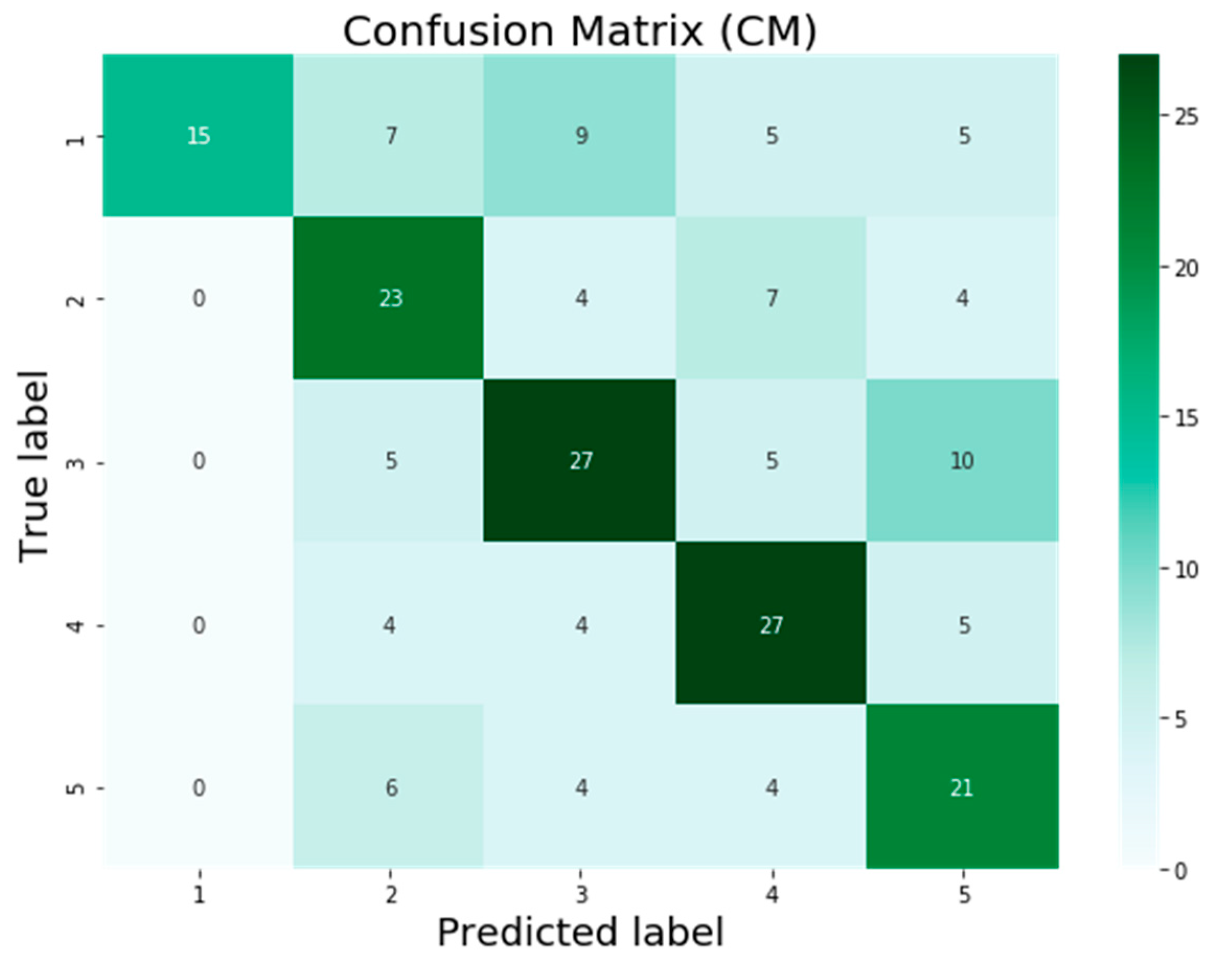
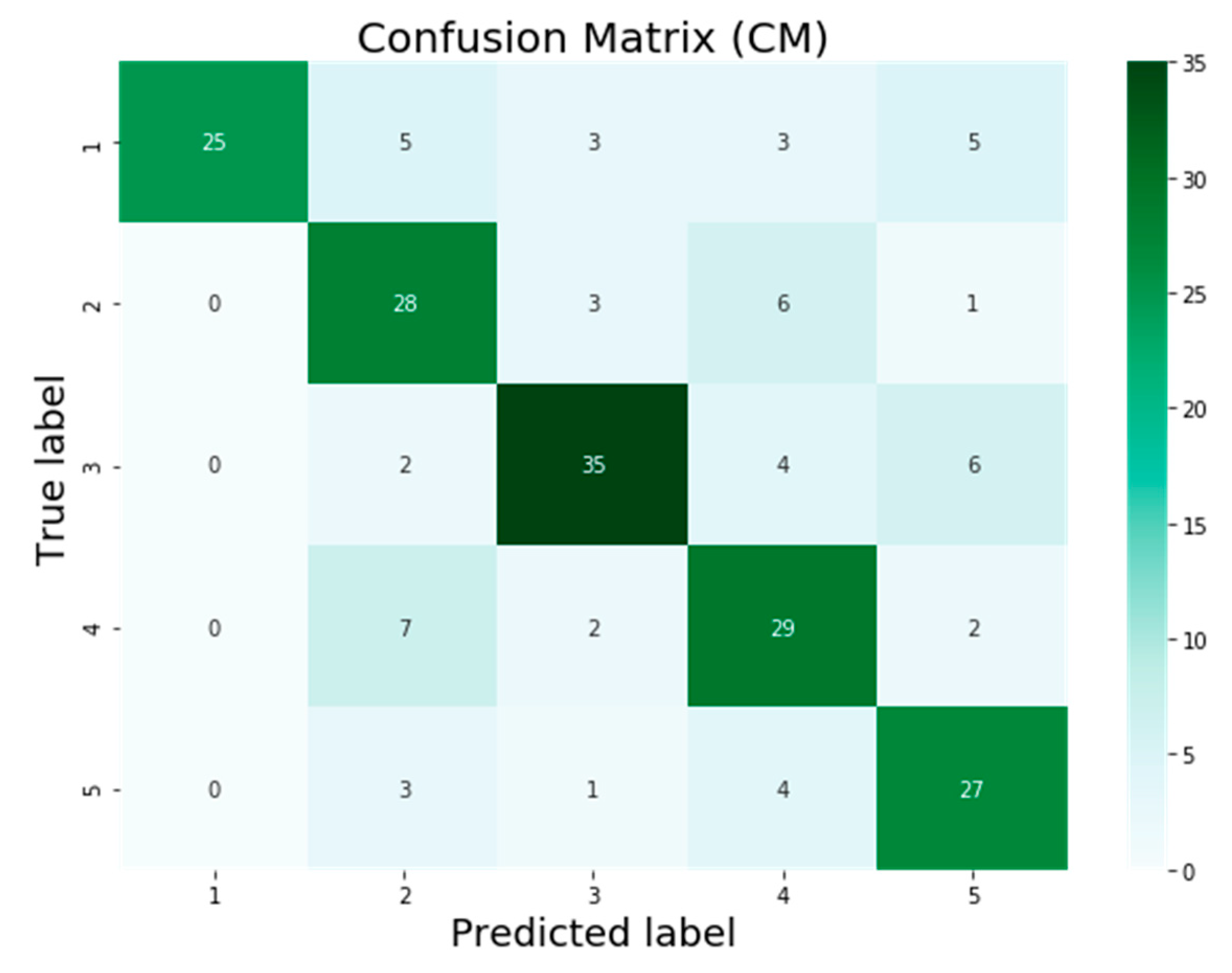
The testing dataset contains a total of 201 photos relating to the first five air pollution level classes such as good, unhealthy, poor, severe, and dangerous. These levels are represented in the classification problem by the numbers 1, 2, 3, 4, and 5. On the basis of the classification results provided by models, a confusion matrix was computed, which is also known as a summary of the results of the predictions made on a classification task or model classification accuracy.

The confusion matrix is presented in Figure 7, Figure 8, Figure 9 and Figure 10 for the four machine learning models SVM, VGG16, InceptionV3, and AQE-net that have been deployed in this study. The numbers 1 to 5 on the horizontal axis reflect the values that were predicted for the test samples, and the values 1 to 5 on the vertical axis represent the actual values of the test samples, respectively. In Figure 7, Figure 8, Figure 9 and Figure 10, the values that are on-diagonal show the number of correctly classified photos, whereas the values that are off-diagonal reflect the number of images with incorrect classifications that vary from the diagonal. After applying the SVM model to the KHI-AQI testing dataset, the confusion matrix is displayed in Figure 7 below. In accordance with the findings, the SVM model successfully classified 113 out of 201 samples, whereas it mistakenly classified 88 samples. In total, there were 201 samples included in the study. 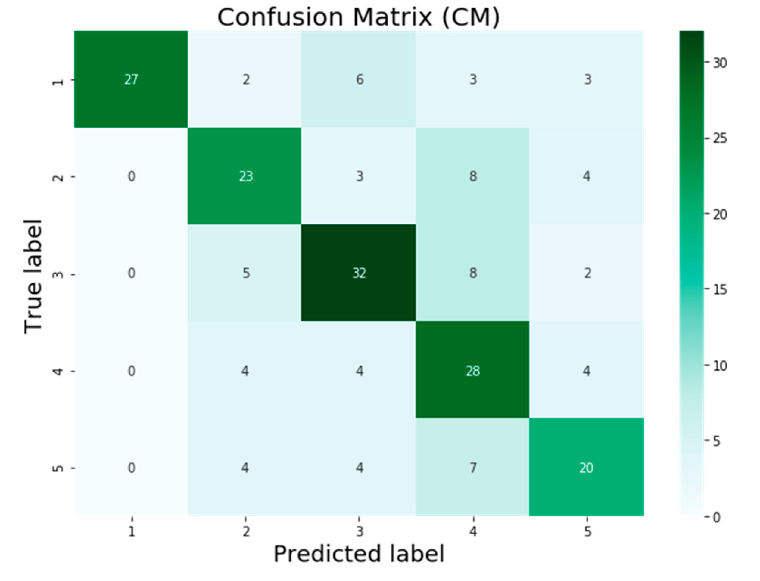The confusion matrix for the KHI-AQI testing dataset using VGG16 is depicted in Figure 8. It was found that 119 of the samples were correctly categorized across all classes, whereas 82 of the samples were misclassified. When compared to the SVM model, the VGG16 algorithm provided six more results that were correctly categorized. After running VGG16 on the same testing dataset, the InceptionV3 algorithm was then applied; the confusion matrix for the InceptionV3 model can be seen in Figure 9. The findings show that out of 201 samples, only 130 were correctly identified using the InceptionV3 model, while 71 samples were incorrectly classified. InceptionV3 had 11 more correctly classified results than VGG16. After first attempting to use the SVM, VGG16, and InceptionV3 models, we finally attempted to validate our proposed model, AQE-Net, by applying it to a testing dataset. Figure 10 presents the classification results using the confusion matrix generated by the AQE-Net model after it was applied to the testing dataset. Out of 201 possible classifications, there were a total of 144 accurate classifications, while there were 57 wrong classifications. AQE-Net was found to have delivered 14 more correct classifications than InceptionV3, according to the findings. When it comes to the categorization of images with AQI levels, the overall confusion matrices on classification results obtained by models indicate that AQE-Net is more superior than other models.

In addition, we evaluated the predictive performance of the SVM, VGG16, InceptionV3, and AQE-Net models with the help of three statistical error metrics known as mean squared error (MSE), mean absolute error (MAE), and mean absolute percentage error (MAPE).

Table 4. MSE, MAE, and MAPE metrics for SVM, VGG16, InceptionV3, and AQE-Net models.

Indicator	SVM	VGG16	InceptionV3	AQE-NET
MSE	1.915	1.910	1.373	1.278
MAE	0.830	0.796	0.626	0.542
MAPE	0.473	0.465	0.326	0.310

shows the MSE, MAE, and MAPE values. When applied to the testing dataset, the SVM model achieved values of 1.915 MSE, 0.830 MAE, and 0.473 MAPE, respectively. The MSE was found to be 1.910, the MAE was 0.796, and the MAPE was found to be 0.465 using the VGG16 model. When compared to the SVM model, the VGG16 model produced fewer errors than the SMV model. Following the application of the VGG16 model, we next applied the InceptionV3 model, and the results of MSE, MAE, and MAPE were 1.373, 0.626, 0.326, respectively, which also reflects fewer errors than were produced by the earlier models, SVM and VGG16. In overall, the AQE-Net model that we proposed had a lower error rate than the other models that were employed in this research. AQE-Net generated estimates of 1.278 MSE, 0.542 MAE, and 0.310 MAPE, respectively, which is quite less than all other models. This shows that the AQE-Net model that we proposed is superior than other models.

4. Discussion

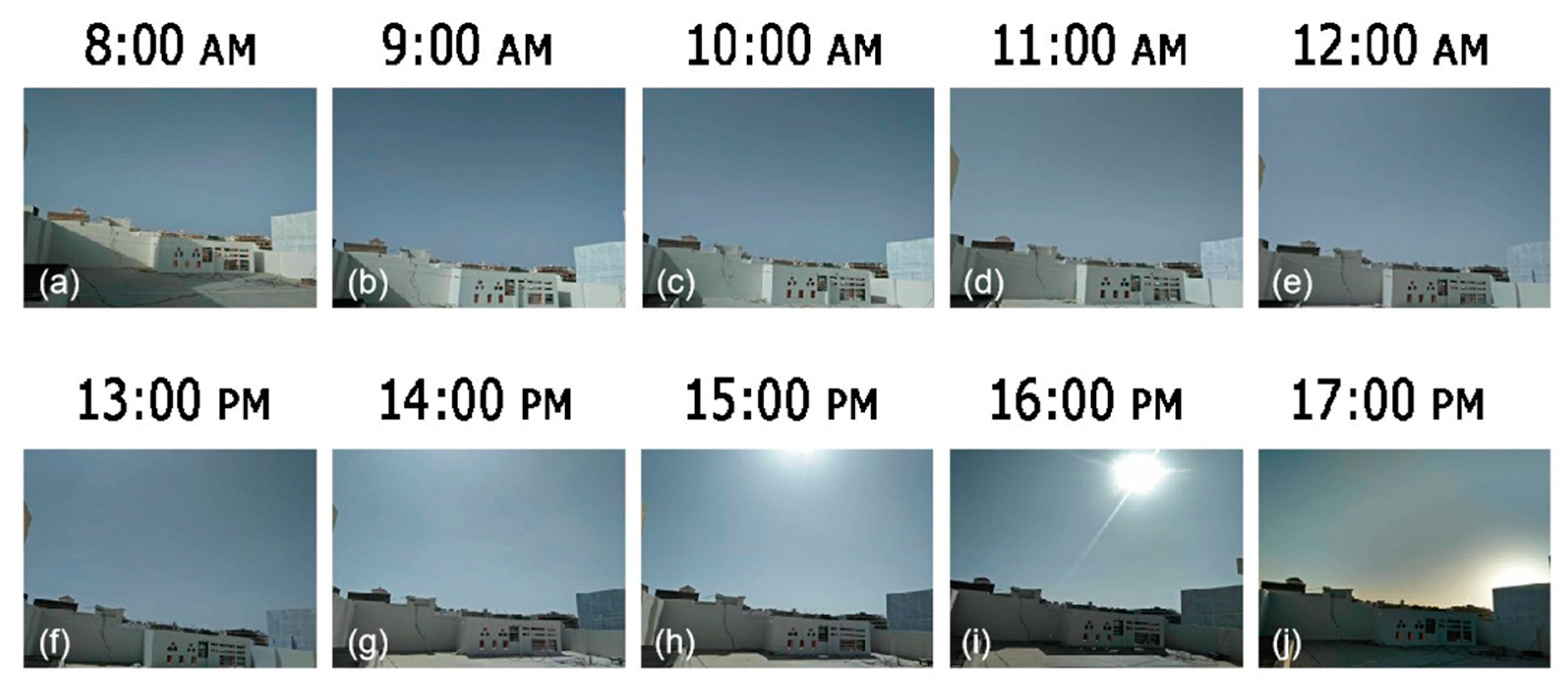
In this study, all of the sample images were taken from fixed-point images, which means the image is acquired at an angle to the sky and that about one-third of the image is taken up by land shared with a building. The goal is to emulate a more frequent and simpler shooting perspective. For monitoring purposes, at least 50% of the frames taken are of the sky. The photographs in this experiment depict scenarios that occur throughout the day (between 7:00 and 19:00). In the evenings, vision is quite poor due to the poor imaging quality. This experimental model is only appropriate for daytime air quality monitoring and is not suitable for nighttime monitoring. Because the model training data is gathered in Karachi, the model’s controllability, dependability, and efficiency are all pretty good in the local region, and the model’s prediction speed and accuracy are all relatively consistent. However, owing to regional climatic and atmospheric variances, the model may not be able to attain the requisite precision in other areas. Our model must be trained and tweaked again with local picture data before it can be used elsewhere. Due to various restrictions, this model will not be able to match the precision of air quality monitoring stations, but it can serve as a complementing tool. The model’s benefit is that individuals can utilize portable image acquisition equipment to get real-time air quality metrics, especially in rural and suburban regions, where the monitoring stations are located far from population centers. Future studies should focus on several areas that can be improved. Different weather conditions significantly impact the brightness or blackness of air quality photographs. The model can be used to directly extract the brightness properties of the picture from the data. Humidity, however, has no discernible influence on photos of air pollution, even though it may impact air quality. Future studies can take into account these considerations to increase model accuracy. Finally, we concentrated our investigation on the AQI, a complete indication of air quality. Future studies could focus on PM2.5 if they wanted to do so.

The dataset size, the initial learning rate, and the number of layers are three training network characteristics that have an impact on the results. This section discusses the impact of the MiniBatchsize training parameter. MiniBatchsize or Batch training involves backpropagating the error of classification via groups of pictures [66]. We propose training the model for various MiniBatchsize values in order to see how this parameter affects the model.

Table 5. MiniBatchsize training results for the value of 60.

No. of Epochs	Number of Iterations	Training Times (s)	Accuracy
3 Epochs	9	12,091.69	0.4866
4 Epochs	12	17,611.09	0.5089
5 Epochs	15	39,255.33	0.5816
6 Epochs	18	42,324.30	0.6514

and

Table 6. MiniBatchsize training results for the value of 10.

No. of Epochs	Number of Iterations	Training Times (s)	Accuracy
3 Epochs	54	11,589.23	0.5866
4 Epochs	72	15,173.47	0.6089
5 Epochs	90	222.349	0.6816
6 Epochs	108	25,934.44	0.7014

give the findings for the values of 60 and 10.

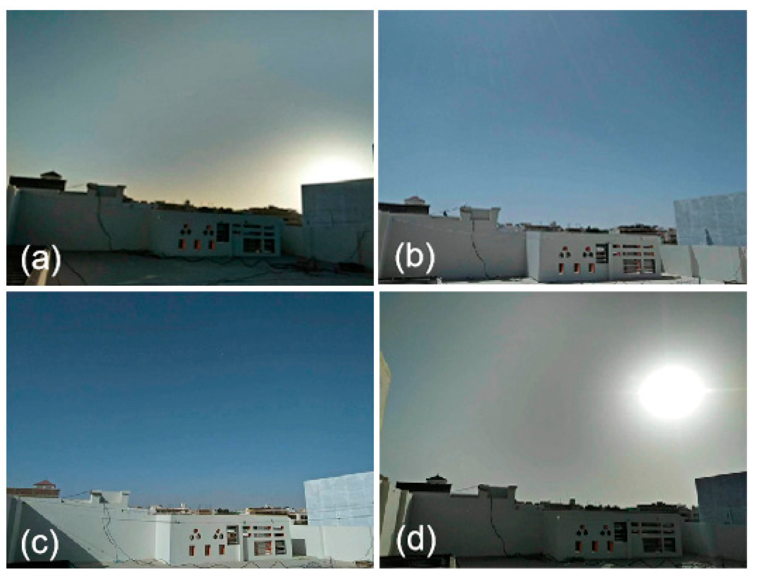
Classification rates during a major training period that ranged between 0.4866 and 0.6541 were obtained by training for various numbers of epochs and a big MiniBatchsize of 60. When compared to the results from Table 5, the decline in rate helps to explain the memorization issue depicted in Figure 11, where unhealthy has been misclassified to the poor category. Images (a), (b), (c), and (d) in Figure 11 are all unhealthy which were mislabeled.

The training for various numbers of epochs results in significant values of the classification rate, as shown in Table 6. These values, which range from 0.5866 to 0.7014, are computed over a training period of 25,934.44 s. Precision in performing the categorization operation is made possible by MiniBatchsize’s low value.

5. Conclusions

In recent decades, air pollution has posed major hazards to human health, prompting widespread public concern. However, ambient pollution measures are expensive, so the geographic coverage of air quality monitoring stations is limited. A low-cost, high-efficiency air quality sensor system benefits human health and air pollution prevention. The AQE-Net air quality assessment model, which is based on deep learning, is proposed in this article. Specifically, deep convolutional neural networks are used to extract feature representational information relating to air quality from scene photos, with the information used to identify air quality levels. A comparative examination of our developed model with traditional and deep learning models, such as SVM, VGG16, and InceptionV3, was also carried out on the KHI-AQI dataset. The experimental findings indicated that the AQE-Net model is superior to other models in classifying photos with AQI levels.

This study has certain limitations. The study used a small sample size and focused only on the Karachi region. Future research should add more datasets and multiple regions to compare the findings with our study. Future studies should take in to account different pollutants, such as PM2.5, PM10, and carbon monoxide (CO₂). Additionally, it is also important to examine seasonal weather conditions and estimate air quality, particularly when visibility is affected due to a foggy environment.

References

1. Ruggieri, M.; Plaia, A. An Aggregate AQI: Comparing Different Standardizations and Introducing a Variability Index. Sci. Total Environ. 2012, 420, 263–272. [Google Scholar] [CrossRef] [PubMed]
2. Kumar, A.; Goyal, P. Forecasting of Daily Air Quality Index in Delhi. Sci. Total Environ. 2011, 409, 5517–5523. [Google Scholar] [CrossRef]
3. Ahmed, M.; Xiao, Z.; Shen, Y. Estimation of Ground PM2.5 Concentrations in Pakistan Using Convolutional Neural Network and Multi-Pollutant Satellite Images. Remote Sens. 2022, 14, 1735. [Google Scholar] [CrossRef]
4. Shi, J.; Wang, X.; Chen, Z. Polluted Humanity: Air Pollution Leads to the Dehumanization of Oneself and Others. J. Environ. Psychol. 2022, 83, 101873. [Google Scholar] [CrossRef]
5. Alizadeh, R.; Soltanisehat, L.; Lund, P.D.; Zamanisabzi, H. Improving Renewable Energy Policy Planning and Decision-Making through a Hybrid MCDM Method. Energy Policy 2020, 137, 111174. [Google Scholar] [CrossRef]
6. Pan, J.; Xue, Y.; Li, S.; Wang, L.; Mei, J.; Ni, D.; Jiang, J.; Zhang, M.; Yi, S.; Zhang, R. PM2.5 Induces the Distant Metastasis of Lung Adenocarcinoma via Promoting the Stem Cell Properties of Cancer Cells. Environ. Pollut. 2022, 296, 118718. [Google Scholar] [CrossRef]
7. Thangavel, P.; Park, D.; Lee, Y.-C. Recent Insights into Particulate Matter (PM2.5)-Mediated Toxicity in Humans: An Overview. Int. J. Environ. Res. Public Health 2022, 19, 7511. [Google Scholar] [CrossRef]
8. Rijal, N.; Gutta, R.T.; Cao, T.; Lin, J.; Bo, Q.; Zhang, J. Ensemble of Deep Neural Networks for Estimating Particulate Matter from Images. In Proceedings of the 2018 IEEE 3rd International Conference on Image, Vision and Computing (ICIVC), Chongqing, China, 27–29 June 2018; pp. 733–738. [Google Scholar]
9. Zhao, K.; He, T.; Wu, S.; Wang, S.; Dai, B.; Yang, Q.; Lei, Y. Research on Video Classification Method of Key Pollution Sources Based on Deep Learning. J. Vis. Commun. Image Represent. 2019, 59, 283–291. [Google Scholar] [CrossRef]
10. Babari, R.; Hautiere, N.; Dumont, E.; Bremond, R.; Paparoditis, N. A Model-Driven Approach to Estimate Atmospheric Visibility with Ordinary Cameras. Atmos. Environ. 2011, 45, 5316–5324. [Google Scholar] [CrossRef] [Green Version]
11. Zhang, C.; Yan, J.; Li, C.; Rui, X.; Liu, L.; Bie, R. On Estimating Air Pollution from Photos Using Convolutional Neural Network. In Proceedings of the 24th ACM International Conference on Multimedia, Amsterdam, The Nederlands, 15–19 October 2016; pp. 297–301. [Google Scholar]
12. Chakma, A.; Vizena, B.; Cao, T.; Lin, J.; Zhang, J. Image-Based Air Quality Analysis Using Deep Convolutional Neural Network. In Proceedings of the 2017 IEEE International Conference on Image Processing (ICIP), Beijing, China, 17–20 September 2017; pp. 3949–3952. [Google Scholar]
13. Baklanov, A.; Mestayer, P.G.; Clappier, A.; Zilitinkevich, S.; Joffre, S.; Mahura, A.; Nielsen, N.W. Towards Improving the Simulation of Meteorological Fields in Urban Areas through Updated/Advanced Surface Fluxes Description. Atmos. Chem. Phys. 2008, 8, 523–543. [Google Scholar] [CrossRef]
14. Pak, U.; Ma, J.; Ryu, U.; Ryom, K.; Juhyok, U.; Pak, K.; Pak, C. Deep Learning-Based PM2.5 Prediction Considering the Spatiotemporal Correlations: A Case Study of Beijing, China. Sci. Total Environ. 2020, 699, 133561. [Google Scholar] [CrossRef]
15. Woody, M.C.; Wong, H.-W.; West, J.J.; Arunachalam, S. Multiscale Predictions of Aviation-Attributable PM2.5 for US Airports Modeled Using CMAQ with Plume-in-Grid and an Aircraft-Specific 1-D Emission Model. Atmos. Environ. 2016, 147, 384–394. [Google Scholar] [CrossRef]
16. Bray, C.D.; Battye, W.; Aneja, V.P.; Tong, D.; Lee, P.; Tang, Y.; Nowak, J.B. Evaluating Ammonia (NH3) Predictions in the NOAA National Air Quality Forecast Capability (NAQFC) Using in-Situ Aircraft and Satellite Measurements from the CalNex2010 Campaign. Atmos. Environ. 2017, 163, 65–76. [Google Scholar] [CrossRef]
17. Zhou, G.; Xu, J.; Xie, Y.; Chang, L.; Gao, W.; Gu, Y.; Zhou, J. Numerical Air Quality Forecasting over Eastern China: An Operational Application of WRF-Chem. Atmos. Environ. 2017, 153, 94–108. [Google Scholar] [CrossRef]
18. Zhong, L.; Hu, L.; Zhou, H. Deep Learning Based Multi-Temporal Crop Classification. Remote Sens. Environ. 2019, 221, 430–443. [Google Scholar] [CrossRef]
19. Giyenko, A.; Palvanov, A.; Cho, Y. Application of Convolutional Neural Networks for Visibility Estimation of CCTV Images. In Proceedings of the 2018 International Conference on Information Networking (ICOIN), Chiang Mai, Thailand, 10–12 January 2018; pp. 875–879. [Google Scholar]
20. Zhang, Q.; Fu, F.; Tian, R. A Deep Learning and Image-Based Model for Air Quality Estimation. Sci. Total Environ. 2020, 724, 138178. [Google Scholar] [CrossRef]
21. Kopp, M.; Tuo, Y.; Disse, M. Fully Automated Snow Depth Measurements from Time-Lapse Images Applying a Convolutional Neural Network. Sci. Total Environ. 2019, 697, 134213. [Google Scholar] [CrossRef]
22. Vahdatpour, M.S.; Sajedi, H.; Ramezani, F. Air Pollution Forecasting from Sky Images with Shallow and Deep Classifiers. Earth Sci. Inform. 2018, 11, 413–422. [Google Scholar] [CrossRef]
23. Soh, P.-W.; Chang, J.-W.; Huang, J.-W. Adaptive Deep Learning-Based Air Quality Prediction Model Using the Most Relevant Spatial-Temporal Relations. IEEE Access 2018, 6, 38186–38199. [Google Scholar] [CrossRef]
24. Yuan, Q.; Shen, H.; Li, T.; Li, Z.; Li, S.; Jiang, Y.; Xu, H.; Tan, W.; Yang, Q.; Wang, J. Deep Learning in Environmental Remote Sensing: Achievements and Challenges. Remote Sens. Environ. 2020, 241, 111716. [Google Scholar] [CrossRef]
25. Wang, B.; Yan, Z.; Lu, J.; Zhang, G.; Li, T. Deep Multi-Task Learning for Air Quality Prediction. In Proceedings of the 25th International Conference on Neural Information Processing, Siem Reap, Cambodia, 13–16 December 2018; pp. 93–103. [Google Scholar]
26. Bo, Q.; Yang, W.; Rijal, N.; Xie, Y.; Feng, J.; Zhang, J. Particle Pollution Estimation from Images Using Convolutional Neural Network and Weather Features. In Proceedings of the 2018 25th IEEE International Conference on Image Processing (ICIP), Athens, Greece, 7–10 October 2018; pp. 3433–3437. [Google Scholar]
27. Chang, F.-J.; Chang, L.-C.; Kang, C.-C.; Wang, Y.-S.; Huang, A. Explore Spatio-Temporal PM2.5 Features in Northern Taiwan Using Machine Learning Techniques. Sci. Total Environ. 2020, 736, 139656. [Google Scholar] [CrossRef]
28. Zhou, Y.; Chang, F.-J.; Chang, L.-C.; Kao, I.-F.; Wang, Y.-S. Explore a Deep Learning Multi-Output Neural Network for Regional Multi-Step-Ahead Air Quality Forecasts. J. Clean. Prod. 2019, 209, 134–145. [Google Scholar] [CrossRef]
29. Zhou, Y.; Chang, L.-C.; Chang, F.-J. Explore a Multivariate Bayesian Uncertainty Processor Driven by Artificial Neural Networks for Probabilistic PM2.5 Forecasting. Sci. Total Environ. 2020, 711, 134792. [Google Scholar] [CrossRef]
30. Li, Y.; Huang, J.; Luo, J. Using User Generated Online Photos to Estimate and Monitor Air Pollution in Major Cities. In Proceedings of the 7th International Conference on Internet Multimedia Computing and Service, Zhangjiajie, China, 19–21 August 2015; pp. 1–5. [Google Scholar]
31. Liu, C.; Tsow, F.; Zou, Y.; Tao, N. Particle Pollution Estimation Based on Image Analysis. PLoS ONE 2016, 11, e0145955. [Google Scholar] [CrossRef]
32. Ma, J.; Li, K.; Han, Y.; Yang, J. Image-Based Air Pollution Estimation Using Hybrid Convolutional Neural Network. In Proceedings of the 2018 24th International Conference on Pattern Recognition (ICPR), Beijing, China, 20–24 August 2018; pp. 471–476. [Google Scholar]
33. Yu, Y.; Samali, B.; Rashidi, M.; Mohammadi, M.; Nguyen, T.N.; Zhang, G. Vision-Based Concrete Crack Detection Using a Hybrid Framework Considering Noise Effect. J. Build. Eng. 2022, 61, 105246. [Google Scholar] [CrossRef]
34. Yu, Y.; Rashidi, M.; Samali, B.; Mohammadi, M.; Nguyen, T.N.; Zhou, X. Crack Detection of Concrete Structures Using Deep Convolutional Neural Networks Optimized by Enhanced Chicken Swarm Algorithm. Struct. Health Monit. 2022, 21, 2244–2263. [Google Scholar] [CrossRef]
35. Heydari, A.; Majidi Nezhad, M.; Astiaso Garcia, D.; Keynia, F.; De Santoli, L. Air Pollution Forecasting Application Based on Deep Learning Model and Optimization Algorithm. Clean Technol. Environ. Policy 2022, 24, 607–621. [Google Scholar] [CrossRef]
36. Muthukumar, P.; Cocom, E.; Nagrecha, K.; Comer, D.; Burga, I.; Taub, J.; Calvert, C.F.; Holm, J.; Pourhomayoun, M. Predicting PM2.5 Atmospheric Air Pollution Using Deep Learning with Meteorological Data and Ground-Based Observations and Remote-Sensing Satellite Big Data. Air Qual. Atmos. Health 2022, 15, 1221–1234. [Google Scholar] [CrossRef]
37. Gilik, A.; Ogrenci, A.S.; Ozmen, A. Air Quality Prediction Using CNN+ LSTM-Based Hybrid Deep Learning Architecture. Environ. Sci. Pollut. Res. 2022, 29, 11920–11938. [Google Scholar] [CrossRef]
38. Kurnaz, G.; Demir, A.S. Prediction of SO2 and PM10 Air Pollutants Using a Deep Learning-Based Recurrent Neural Network: Case of Industrial City Sakarya. Urban Clim. 2022, 41, 101051. [Google Scholar] [CrossRef]
39. Hu, K.; Guo, X.; Gong, X.; Wang, X.; Liang, J.; Li, D. Air Quality Prediction Using Spatio-Temporal Deep Learning. Atmos. Pollut. Res. 2022, 13, 101543. [Google Scholar] [CrossRef]
40. Mengara Mengara, A.G.; Park, E.; Jang, J.; Yoo, Y. Attention-Based Distributed Deep Learning Model for Air Quality Forecasting. Sustainability 2022, 14, 3269. [Google Scholar] [CrossRef]
41. AirNow. Available online: https://www.airnow.gov/ (accessed on 10 February 2022).
42. Fukushima, K.; Miyake, S. Neocognitron: A Self-Organizing Neural Network Model for a Mechanism of Visual Pattern Recognition. In Competition and Cooperation in Neural Nets; Springer: Berlin, Germany, 1982; pp. 267–285. [Google Scholar]
43. LeCun, Y.; Boser, B.; Denker, J.S.; Henderson, D.; Howard, R.E.; Hubbard, W.; Jackel, L.D. Backpropagation Applied to Handwritten Zip Code Recognition. Neural Comput. 1989, 1, 541–551. [Google Scholar] [CrossRef]
44. Rivenson, Y.; Liu, T.; Wei, Z.; Zhang, Y.; de Haan, K.; Ozcan, A. PhaseStain: The Digital Staining of Label-Free Quantitative Phase Microscopy Images Using Deep Learning. Light Sci. Appl. 2019, 8, 1–11. [Google Scholar] [CrossRef] [PubMed] [Green Version]
45. Liu, Y.; Racah, E.; Correa, J.; Khosrowshahi, A.; Lavers, D.; Kunkel, K.; Wehner, M.; Collins, W. Application of Deep Convolutional Neural Networks for Detecting Extreme Weather in Climate Datasets. arXiv 2016, arXiv:1605.01156. [Google Scholar]
46. Shen, Y.; He, X.; Gao, J.; Deng, L.; Mesnil, G. Learning Semantic Representations Using Convolutional Neural Networks for Web Search. In Proceedings of the 23rd International Conference on World Wide Web, Seoul, Republic of Korea, 7–11 April 2014; pp. 373–374. [Google Scholar]
47. Rivenson, Y.; Zhang, Y.; Günaydın, H.; Teng, D.; Ozcan, A. Phase Recovery and Holographic Image Reconstruction Using Deep Learning in Neural Networks. Light Sci. Appl. 2018, 7, 17141. [Google Scholar] [CrossRef] [Green Version]
48. Clark, C.; Storkey, A. Training Deep Convolutional Neural Networks to Play Go. In Proceedings of the International Conference on Machine Learning, Lille, France, 7–9 July 2015; pp. 1766–1774. [Google Scholar]
49. Rahmani, B.; Loterie, D.; Konstantinou, G.; Psaltis, D.; Moser, C. Multimode Optical Fiber Transmission with a Deep Learning Network. Light Sci. Appl. 2018, 7, 1–11. [Google Scholar] [CrossRef] [PubMed] [Green Version]
50. Zeiler, M.D.; Fergus, R. Visualizing and Understanding Convolutional Networks. In Proceedings of the European Conference on Computer Vision, Zurich, Switzerland, 6–12 September 2014; pp. 818–833. [Google Scholar]
51. Szegedy, C.; Liu, W.; Jia, Y.; Sermanet, P.; Reed, S.; Anguelov, D.; Erhan, D.; Vanhoucke, V.; Rabinovich, A. Going Deeper with Convolutions. In Proceedings of the IEEE Conference on Computer Vision and Pattern Recognition, Boston, MA, USA, 7–12 June 2015; pp. 1–9. [Google Scholar]
52. LeCun, Y.; Bottou, L.; Bengio, Y.; Haffner, P. Gradient-Based Learning Applied to Document Recognition. Proc. IEEE 1998, 86, 2278–2324. [Google Scholar] [CrossRef] [Green Version]
53. Howard, A.G.; Zhu, M.; Chen, B.; Kalenichenko, D.; Wang, W.; Weyand, T.; Andreetto, M.; Adam, H. Mobilenets: Efficient Convolutional Neural Networks for Mobile Vision Applications. arXiv 2017, arXiv:1704.04861. [Google Scholar]
54. Simonyan, K.; Zisserman, A. Very Deep Convolutional Networks for Large-Scale Image Recognition. arXiv 2014, arXiv:1409.1556. [Google Scholar]
55. Sermanet, P.; Eigen, D.; Zhang, X.; Mathieu, M.; Fergus, R.; LeCun, Y. Overfeat: Integrated Recognition, Localization and Detection Using Convolutional Networks. Eprint Arxiv. arXiv 2013, arXiv:1312.6229. [Google Scholar]
56. Huang, G.; Liu, Z.; Van Der Maaten, L.; Weinberger, K.Q. Densely Connected Convolutional Networks. In Proceedings of the IEEE Conference on Computer Vision and Pattern Recognition, Honolulu, HI, USA, 21–26 July 2017; pp. 4700–4708. [Google Scholar]
57. He, K.; Zhang, X.; Ren, S.; Sun, J. Spatial Pyramid Pooling in Deep Convolutional Networks for Visual Recognition. IEEE Trans. Pattern Anal. Mach. Intell. 2015, 37, 1904–1916. [Google Scholar] [CrossRef] [PubMed] [Green Version]
58. He, K.; Zhang, X.; Ren, S.; Sun, J. Deep Residual Learning for Image Recognition. In Proceedings of the IEEE Conference on Computer Vision and Pattern Recognition, Las Vegas, NV, USA, 27–30 June 2016; pp. 770–778. [Google Scholar]
59. Krizhevsky, A.; Sutskever, I.; Hinton, G.E. Imagenet Classification with Deep Convolutional Neural Networks. Adv. Neural Inf. Process. Syst. 2012, 25, 1097–1105. [Google Scholar] [CrossRef] [Green Version]
60. Vaswani, A.; Shazeer, N.; Parmar, N.; Uszkoreit, J.; Jones, L.; Gomez, A.N.; Kaiser, Ł.; Polosukhin, I. Attention Is All You Need. In Proceedings of the 31st Conference on Neural Information Processing Systems (NIPS 2017), Long Beach, CA, USA, 4–9 December 2017. [Google Scholar]
61. Lin, Z.; Feng, M.; dos Santos, C.N.; Yu, M.; Xiang, B.; Zhou, B.; Bengio, Y. A Structured Self-Attentive Sentence Embedding. arXiv 2017, arXiv:1703.03130. [Google Scholar]
62. Ioffe, S.; Szegedy, C. Batch Normalization: Accelerating Deep Network Training by Reducing Internal Covariate Shift. In Proceedings of the International Conference on Machine Learning, Lille, France, 7–9 July 2015; pp. 448–456. [Google Scholar]
63. Nair, V.; Hinton, G.E. Rectified Linear Units Improve Restricted Boltzmann Machines. In Proceedings of the 27th International Conference on Machine Learning (ICML), Haifa, Israel, 21–24 June 2010. [Google Scholar]
64. Paszke, A.; Gross, S.; Chintala, S.; Chanan, G.; Yang, E.; DeVito, Z.; Lin, Z.; Desmaison, A.; Antiga, L.; Lerer, A. Automatic Differentiation in Pytorch. In Proceedings of the 31st Conference on Neural Information Processing Systems (NIPS 2017), Long Beach, CA, USA, 4–9 December 2017. [Google Scholar]
65. He, K.; Zhang, X.; Ren, S.; Sun, J. Delving Deep into Rectifiers: Surpassing Human-Level Performance on Imagenet Classification. In Proceedings of the IEEE International Conference on Computer Vision, Santiago, Chile, 7–13 December 2015; pp. 1026–1034. [Google Scholar]
66. Jmour, N.; Zayen, S.; Abdelkrim, A. Convolutional Neural Networks for Image Classification. In Proceedings of the 2018 International Conference on Advanced Systems and Electric Technologies (IC_ASET), Hammamet, Tunisia, 22–25 March 2018; pp. 397–402. [Google Scholar]
Figure 1. Karachi map with its districts and research area.
Remotesensing 14 05732 g001
Figure 2. Scene image examples from the KHI image library.
Remotesensing 14 05732 g002
Figure 3. AQI data from the monitoring station for Karachi City.
Remotesensing 14 05732 g003
Figure 4. CNN’s fundamental structure.
Remotesensing 14 05732 g004
Figure 5. The AQE-Net model architecture for air quality index (AQI).
Remotesensing 14 05732 g005
Figure 6. Spatial and context attention block.
Remotesensing 14 05732 g006
Figure 7. Confusion matrix (SVM).
Remotesensing 14 05732 g007
Figure 8. Confusion matrix (VGG16).
Remotesensing 14 05732 g008
Figure 9. Confusion matrix (InceptionV3).
Remotesensing 14 05732 g009
Figure 10. Confusion matrix (AQE-Net).
Remotesensing 14 05732 g010
Figure 11. Test samples from testing dataset, (ad) images are unhealthy category.
Remotesensing 14 05732 g011