
Multiple Band Prioritization Criteria-Based Band Selection for Hyperspectral Imagery

1
School of Information Science and Technology, Dalian Maritime University, Dalian 116026, China
2
Peng Cheng Laboratory, Shenzhen 518000, China
*
Author to whom correspondence should be addressed.
Remote Sens. 2022, 14(22), 5679; https://doi.org/10.3390/rs14225679
Submission received: 4 August 2022
/
Revised: 2 November 2022
/
Accepted: 3 November 2022
/
Published: 10 November 2022
(This article belongs to the Section Remote Sensing Image Processing)
Abstract
:Band selection (BS) is an effective pre-processing way to reduce the redundancy of hyperspectral data. Specifically, the band prioritization (BP) criterion plays an essential role since it can judge the importance of bands from a particular perspective. However, most of the existing methods select bands according to a single criterion, leading to incomplete band evaluation and insufficient generalization against different data sets. To address this problem, this work proposes a multi-criteria-based band selection (MCBS) framework, which innovatively treats BS as a multi-criteria decision-making (MCDM) problem. First, a decision matrix is constructed based on several typical BPs, so as to evaluate the bands from different focuses. Then, MCBS defines the global positive and negative idea solutions and selects bands according to their relative closeness to these solutions. Since each BP has a different capability to discriminate the bands, two weight estimation approaches are developed to adaptively balance the contributions of various criteria. Finally, this work also provides an extended version of MCBS, which incorporates the subspace partition strategy to reduce the correlation of the selected bands. In this paper, the classification task is used to evaluate the performance of the selected band subsets. Extensive experiments on three public data sets verify that the proposed method outperforms other state-of-the-art methods.
1. Introduction
Hyperspectral images (HSIs) can provide abundant spectral information from hundreds of narrow and contiguous channels, which enables better spectral characterization of the objects and improves the detection and recognition capabilities [1]. Therefore, HSI gets widely used in various research fields, such as mineral exploration [2,3], environmental protection [4,5], and medical diagnosis [6,7]. However, the nanoscale spectral resolution also brings many problems, including data redundancy, high computational complexity, and the curse of dimensionality [8]. As a result, dimensionality reduction (DR) is considered to be a necessary pre-processing step for hyperspectral data analysis [9].
In general, the existing DR methods for HSI are mainly composed of feature extraction [10,11,12,13,14,15,16,17] and band selection (BS) [18,19,20,21,22,23,24,25,26,27,28,29,30,31,32,33,34,35,36]. Feature extraction usually extracts the required feature information by projecting the raw data from the high-dimensional space to the low-dimensional space. The two most fundamental methods are principal component analysis (PCA) [10] and Fisher’s linear discriminant analysis (LDA) [11], respectively. Based on the above, the improved versions have been proposed, such as kernel PCA [12], local Fisher’s discriminant analysis (LFDA) [13] and subspace LDA [14]. In addition, some manifold learning approaches including locally linear embedding (LLE) [15], locality preserving projection (LPP) [16], and maximum margin projection (MMP) [17] are also some of the more advanced feature extraction techniques available. As for BS, it aims to select the most representative and informative bands with small inter-band correlation, without destroying the physical significance of the raw data [18]. In addition, the selected bands could be obtained directly from the imaging process, which can effectively reduce the computational time of the subsequent tasks. Thus, BS is generally considered to be preferable for feature extraction in most cases [19].
Due to the acquisition of the labeled HSI being a difficult task, unsupervised BS methods attracted more attention compared to supervised methods. Currently, the typically unsupervised BS methods can be roughly divided into ranking-based methods [20,21,22,23], clustering-based methods [24,25,26,27], and methods based on other modes (e.g., subspace partition (SP) [28,29,30], deep learning [31,32,33] and sparse representation [34,35]). Ranking-based methods evaluate the importance of each band through certain band prioritization (BP) criteria, the representative methods include information entropy (IE) [20], maximum variance principal component analysis (MVPCA) [21], constrained band selection (CBS) [22], saliency-based band selection (SSBS) [23], etc. Clustering-based methods cluster the bands according to the similarity measures and the band nearest to each clustering center is selected to constitute the band subset. The classic methods are hierarchical clustering [24], Ward’s linkage strategy using divergence (WaLuDi) [25], enhanced fast density-peak-based clustering (E-FDPC) [26], and optimal clustering framework (OCF) [27], etc. Ranking-based BS generally has high computational efficiency but ignores the correlation between bands, and clustering BS could significantly reduce redundancy, but some informative bands may be dropped. To address these issues, some SP-based BS approaches combine the advantages of ranking and clustering methods. They first divide the original data into different subspaces and then select the most representative bands according to a given ranking-based BP. For instance, Wang et al. [28] proposed the adaptive subspace partition strategy (ASPS), which defines the partition points based on the ratio of intra-class distance to inter-class distance. Sun et al. [29] proposed constrained target BS with subspace partition (CTSPBS) for the target detection task, where the forward minimum variance strategy and the backward maximum variance strategy are utilized to select the representative bands. Recently, Wang et al. [30] proposed a fast neighborhood grouping BS method (FNGBS), which selected the band with the largest product of entropy and local density from each subspace. In addition, some BS methods using deep learning are designed to fully exploit the complex nonlinear relationships in HSI, such as BS-Nets [31], attention-based autoencoders (AAE) [32], global–local spectral weight network based on attention (GLSWA) [33], but their performance is still limited by the hyper-parameters and stochastic processes.
To sum up, the BP criterion plays an important role whether in ranking-based BS, SP-based BS or other kinds of BS methods. However, most existing methods measure the bands by a single criterion, leading incomplete band evaluation and insufficient generalization ability against different data sets. In this context, Wang et al. [36] proposed hypergraph spectral clustering BS (HSCBS), which provides a hypergraph construction way to combine three different BP criteria, including IE, MVPCA and E-FDPC. Das et al. [37] developed sparsity regularized deep subspace clustering (SRDSC) BS, where a multi-criteria-based strategy is introduced to identify the representative bands from the clusters. These approaches demonstrate that the combination of different BP criteria allows a more comprehensive band assessment and improves classification accuracy. Nonetheless, they are still limited by the selection of the employed criteria. Additionally, since each criterion has a different capability to judge the bands, the relative importance between multiple criteria and their fusion manner also deserves further discussion.
Motivated by the above descriptions, in this article, we take the BS process as a multi-criteria decision-making (MCDM) problem. MCDM technique is derived from operations research, which is to compare the alternatives with the help of binary or fuzzy relations [38,39]. In the case of MCDM, multiple criteria are described as quantitative or qualitative indices and weighted in appropriate ways, then the evaluation results with different focuses are used to aggregate the final decision by various methods. There are many sophisticated methods for MCDM, such as analytic hierarchy process (AHP) [40], elimination and choice expressing reality (ELECTRE) [41] and order preference by similarity to ideal solution (TOPSIS) [42], which have been successfully applied in disaster prediction [43], cloud computing [44], smart grid [45], human–computer interaction [46] and many other scientific fields. Despite little related research before, MCDM is considered to be an effective tool for BS because of two main reasons. On the one hand, it is a reliable technique for integrating multiple BP standards, allowing a more comprehensive band evaluation. On the other hand, the weight estimation in MCDM enables the measurement of the relative importance of multiple criteria and make them trade-off.
By means of MCDM, we propose a novel unsupervised BS method, i.e., multi-criteria-based BS (MCBS), to select bands by multiple BP criteria with different focuses. In contrast to most existing methods, MCBS can be regarded as a general framework integrating multiple BP criteria, which is expected to achieve more comprehensive band evaluation and stronger robustness to different data sets. The main contributions are listed below.
- This work regards BS as an MCDM problem and proposes a novel unsupervised BS method for hyperspectral imagery, namely MCBS. The integration of multiple BPs enables a comprehensive band evaluation, and makes MCBS more robust against different data sets.
- To balance the contributions of various BP criteria, MCBS also provides two weight estimation approaches, which can adaptively attach weight to each criterion from information diversity and correlation perspectives.
- This work also provides an extended version of MCBS, which incorporates the SP strategy to further reduce the correlation of the selected bands. Extensive experiments demonstrate its superiority over the state-of-the-art methods.
2. MCBS Framework
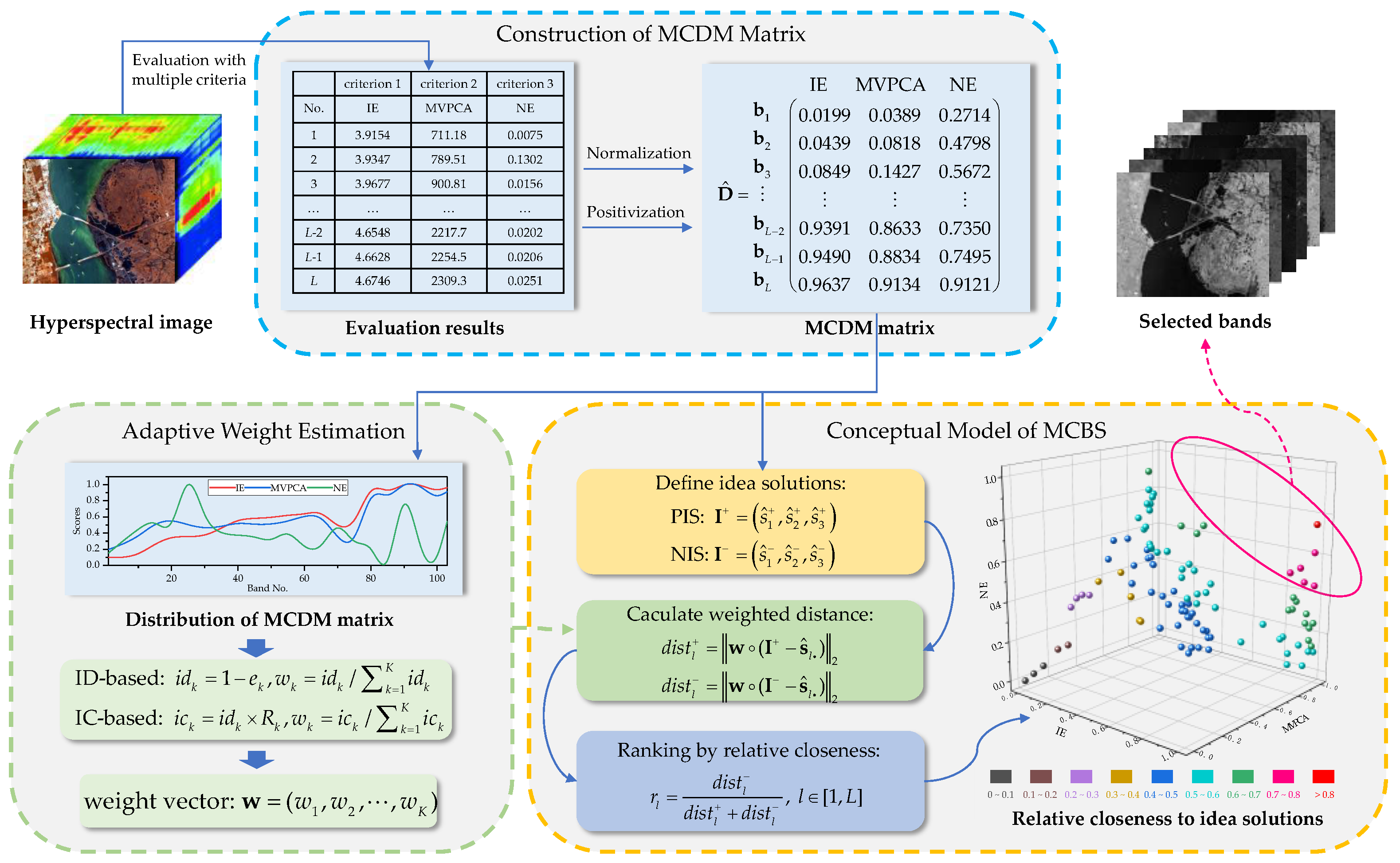
This section details the proposed framework, MCBS, whose flowchart is shown in Figure 1. The basic principle is to treat hyperspectral BS as an MCDM problem with L alternatives and K criteria, where L and K represent the number of total bands and employed BP criteria, respectively. Specifically, the proposed method is described in three aspects, including the construction of MCDM matrix, conceptual mode of MCBS, and weight estimation approaches. Finally, this section also provides a more sophisticated extended version, SP-MCBS, to achieve better performance.
2.1. Construction of MCDM Matrix
MCBS allows the integration of multiple BP criteria, which can evaluate bands from various perspectives and generate a final band priority sequence. Before performing BS, it is necessary to select several criteria as the baselines and construct the corresponding MCDM matrix. In addition, it is worth noting that these baselines should be typical ranking-based methods, and evaluate the bands from as diverse perspectives as possible, so that the decision matrix would have more comprehensive and valuable information. In this article, we choose IE [20], MVPCA [21] and noise estimation (NE) [28] to measure the entropy, variance and noise level of the bands, respectively.
Suppose denotes the raw HSI, where L indicates the total number of bands, N represents the number of pixels in each band, and means the N-dimensional column vector of l-th band. Then, the baselines and the construction of the MCDM matrix are briefly described as follows.
(1) IE [20]: Information entropy is commonly used in BS to describe information richness. Generally speaking, the higher the entropy of the band, the more the amount of information it contains. IE is less sensitive to noisy bands, which makes it more robust in handling data polluted by noises. Here, the score of IE is defined as:
where is value of grayscale color, represents the set of all grayscale values on band , denotes the probability density function, whose calculation could be accelerated by the grayscale histogram.
(2) MVPCA [21]: MVPCA first constructs a data–sample covariance matrix, then decomposes it with eigenvalues to obtain a loading factor matrix, and finally, determines the band priority based on this matrix. In MVPCA, the bands are prioritized by their variances, where the variance is the greater means the greater the amount of information is contained in the bands. The ranking variance of the band is obtained by
where denotes the reflectance value of the n-th pixel on , and represents the mean value of this band. Compared to IE, MVPCA evaluates the amount of information in the band from another perspective, but it is greatly affected by noise.
(3) NE [28]: NE is introduced in ASPS, which allows rapid estimation of the noise level of each band image. The band image is first divided into small blocks with equal size of pixels, and then the global noise level is estimated according to the local variance of these blocks. The calculation of local variance, LV, can be simplified as
where is the value of the i-th pixel, and denotes the mean variance of this block. Then, the difference between the maximum and minimum LV of all blocks for each band image is divided into z bins with equal width, i.e., , where maxV is the maximum variance, minV denotes the minimum variance, and α stands for the partition granularity (α = 3 in this article).
Further, all blocks are allotted into these bins in accordance with the values of LV. The bin with the largest number of blocks corresponds to the estimated noise of the band image. Additionally, the NE value of each band is obtained, i.e., . Here, NE is briefly introduced as a published work. If necessary, please refer to [28] for in-depth review. For the proposed MCBS, the integration of NE is expected to improve its robustness against noises.
(4) MCDM Matrix Construction: As mentioned above, MCBS considers BS as a MCDM problem with L alternatives (bands) and K criteria (obviously K = 3 in this article). Thus, the decision matrix can be expressed as
where , and denote the three baseline criteria: IE, MVPCA and NE, respectively, and represents the score of l-th band evaluated by the criterion . It is worth noting that the MCDM matrix requires positivizing each evaluation criterion. Since NE is a negative criterion, the score of NE is taken as its inverse.
Then, the matrix D needs to be normalized in order to transform the various criteria into non-dimensional versions, thus allowing comparison across them. In this article, the decision matrix D is normalized according to
As a result, a normalized decision matrix containing the scores of all bands regarding three baselines methods is constructed as
2.2. Conceptual Mode of MCBS
The constructed MCDM matrix combines K criteria (K = 3 in this paper), and comprehensively measures the importance of bands from different focuses. However, there are still two key issues that need to be addressed: (1) a global BP measurement should be defined to rank the bands, (2) each criterion has a different capability to judge the bands, so it is necessary to know its relative importance. For the former, drawing on the idea of TOPSIS [42], MCBS defines the global positive ideal solution (PIS) and negative ideal solution (NIS), and ranks the bands by their relative closeness to the ideal solutions. For the latter, MCBS provides two data-driven ways to measure the evaluative capability of the baseline criteria and adaptively weighted them.
First, the ideal solutions, PIS and NIS are defined as
Here, and represent PIS and NIS, respectively, which correspond to the best and worst evaluations achievable for all bands in an ideal condition.
In , the row vector indicates the performance of the l-th band corresponding to K baseline criteria. Based on the concept of TOPSIS, MCBS selects the band with the shortest distance from PIS and the farthest distance from NIS. Specifically, the distances of the l-th band to PIS and NIS are calculated by
where “∘” is Hadamard product, representing the elementwise multiplication. The distance with idea solutions is weighted so as to take into account the relative importance of each criterion. Here, is the weight vector, and denotes the weight for the k-th evaluation criterion, which subjects to . The detailed weighting calculations are presented in Section 2.3.
Finally, MCBS ranks the bands according to its relative closeness to ideal solutions, which is calculated as:
The larger the is, the higher the priority of the band. As a result, MCBS obtains a final BP sequence based on multiple criteria.
2.3. Adaptive Weight Estimation by MCBS
As mentioned previously, each criterion has a different capability to evaluate the bands, so and are weighted by to describe the relative importance of the criteria. The calculation of should be adaptive for the employed data, because the relative importance varies when processing different data sets. Thus, MCBS provides two weight estimation approaches, namely the information diversity-based approach (ID) and inter-criteria correlation-based approach (IC). These two approaches measure the importance of a criterion by analyzing the data distribution of its evaluation results, which are both objective weight estimation methods.
2.3.1. ID-Based Weight Estimation
For the ID-based method, it considers that the higher the ID of evaluation results, the better the ability of a criterion to discriminate the bands. For example, if the evaluation results of a criterion are very similar for all bands, which means that it does not provide much differentiation information for BS, and its weight should be very low. In contrast, the criterion with a higher ID should be considered more important. In particular, the degree of diversity is defined as
where denotes the entropy of the k-th criterion. In informatics theory, entropy is a measurement of information uncertainty. The larger the entropy, the lower the degree of information uncertainty and the smaller the ID; on the contrary, the smaller the entropy, the more uncertain the information, and the higher the degree of information diversity. Here, the entropy of each criterion is calculated by
where is a constant term to ensure . Finally, the weight of the k-th criterion is expressed as
2.3.2. IC-Based Weight Estimation
The ID-based method has a limitation that it does not take into account the dependencies between criteria, assuming that each criterion evaluates bands from an individual perspective. However, although the selection of baseline BP criteria is as diverse as possible, some criteria show dependence on each other. Therefore, when the results of two or more criteria are highly correlated, their importance to BS should be appropriately reduced. Instead, a relatively independent criterion should attract more attention.
Based on the above descriptions, the weighting factor of the IC-based method, , is constructed as
where denotes the degree of the independence of a criterion. The larger the , the more independent the criterion is. Additionally, it is defined as
where represents the linear correlation coefficient between the evaluation results of the k-th and the m-th criteria.
Finally, the IC-based method constructs the weight vector according to
2.4. Extended Version of MCBS
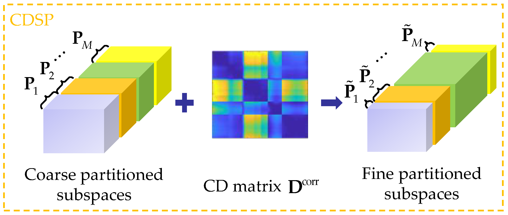
Although the integration of multiple BP criteria enables a more comprehensive assessment of the bands, MCBS is still a ranking-based BS with the problem of ignoring band correlation. In this section, a more sophisticated extended version, SP-MCBS, is proposed to reduce the internal correlation of the selected bands and thus achieve better classification performance. SP-MCBS is a combination of MCBS and subspace partition based on correlation distance (CDSP). In particular, CDSP is introduced in our previous work [29], which could adaptively divide the ordered hyperspectral bands into several uncorrelated subsets.
2.4.1. CDSP
CDSP consists of two main steps, coarse partition and fine partition. Figure 2 gives a schematic of CDSP. In the first step, the hyperspectral data is roughly divided into M subsets , , with equal size Z, where M is the number required bands, and Z is determined by
In the second step, a correlation distance matrix , is constructed first. Here, represents the correlation distance between and , and is calculated by
where denotes the Pearson correlation coefficient between bands. According to , CDSP defines inter-class correlation distance and intra-class correlation distance to guide the SP. Finally, the partition point t between every two adjacent subspaces is determined by the following objective function
Here, CDSP is briefly introduced as a related work. If necessary, please refer to [29] for an in-depth review.
2.4.2. SP-MCBS
After CDSP, the raw hyperspectral data is divided into several uncorrelated subspaces , . According to Equation (11), MCBS considers that a band with the larger , the higher its score across the multiple criteria. Therefore, it provides an overall BP measure as
where the notation “≻” is used to indicate “superior to”. Then, the band with the largest in each subspace is selected as a candidate band, which is obtained by
Thus, the selected band subset are generated. The detailed implementation of SP-MCBS Algorithm 1 is as follows.
| Algorithm 1 SP-MCBS |
| Input: HSI data , the number of selected bands M |
| Output: The selected band subset |
|
3. Experiments and Results
In this paper, the classification task is used to evaluate the performance of the selected band subsets. This section first introduces the experimental setup, including the data sets, classification settings and the number of selected bands. Second, the effectiveness of MCBS is verified by comparing it with its baseline methods, and the performance of two weight estimation methods is also analyzed. Then, a comprehensive comparison of classification performance is shown to see whether SP-MCBS is superior to the other state-of-the-art methods. Finally, we discuss the results from several different aspects.
3.1. Experimental Setup
3.1.1. Data Sets
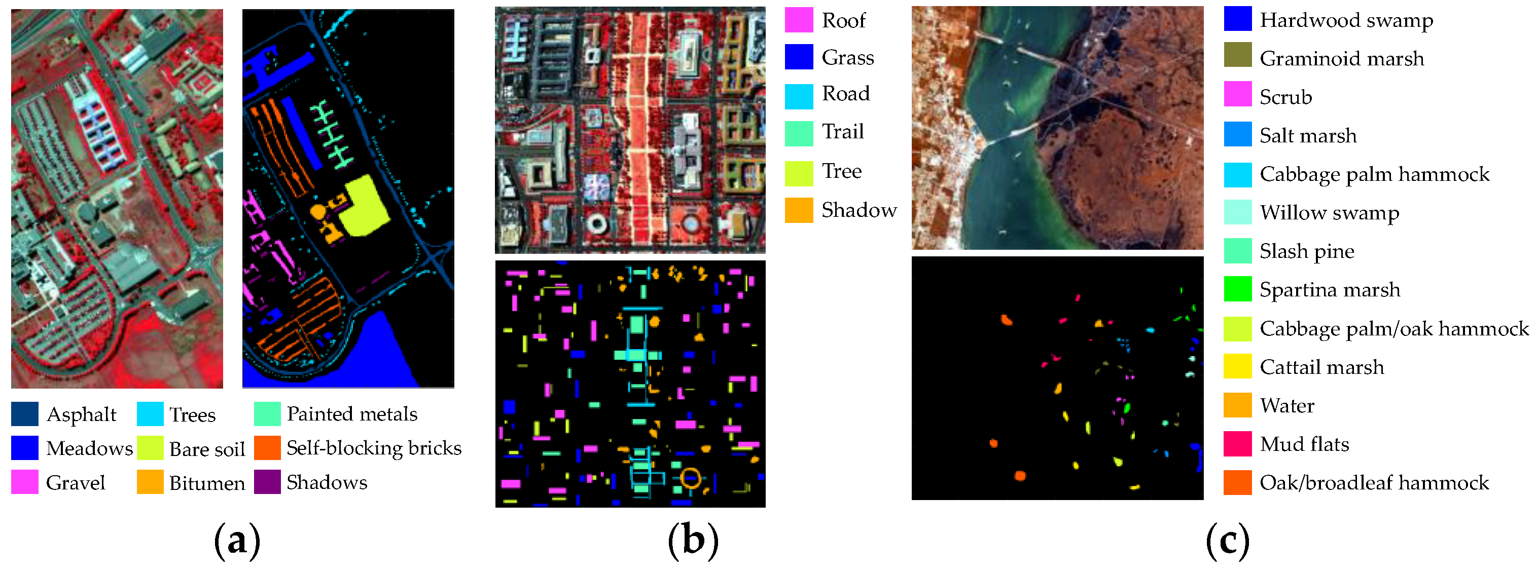
Three real-world public HSIs are used in our experiments, namely Pavia University, Washington DC Mal and Kennedy Space Center (KSC). The details are displayed in Figure 3 and listed in Table 1.
(1) Pavia University: The Pavia University scene was captured by the reflective optics system imaging spectrometer (ROSIS) sensor over Pavia in 2002, which consists of 610 × 340 pixels and 115 bands of 4 nm width. After removing some bands with lower SNR, the number of spectral bands employed in experiments is 103. The ground-truth of this data set includes nine classes of interest for classification.
(2) Washington DC Mall: The Washington DC Mall scene was collected by the hyperspectral digital imagery collection experiment (HYDICE) airborne sensor, comprises 210 spectral bands with 10 nm spectral resolution. There are 191 bands remaining after omitting the bands in the region where atmosphere is opaque. In this article, a 280 × 307 pixels sub-image of the data is used for proper assessment, which includes six classes of interest.
(3) Kennedy Space Center (KSC): The KSC scene was gathered by the Airborne Visible Infra-Red Imaging Spectrometer (AVIRIS) sensor over the Kennedy Space Center, Florida in 1996. This data set consists of 176 bands with the size of 512 × 614 pixels after removing water absorption and low SNR bands. The spectral resolution is 10 nm. For classification purposes, 13 classes representing the various land cover types are defined for the site.
3.1.2. Classifier and Parameter Settings
During the experiments, two typical classifiers, support vector machine (SVM) and k-nearest neighborhood (KNN) are employed to compare the performance of the BS algorithms. In our experiments, the SVM classifier is conducted with the RBF kernel, and the same parameters are set to ensure the accuracy of the experiment. Specifically, the penalty factor and gamma of SVM are 1 × 10⁴ and 0.5, respectively. In addition, the parameter K is set to three for all classification validation experiments about KNN. For each category, 10% of the samples are randomly selected as the training samples and the rest for testing. In addition, overall accuracy (OA) and average accuracy (AA) are used as classification measures. Moreover, the final results are obtained by averaging 10 individual runs to reduce the effect of the random selection of training samples. Finally, the parameters of all comparison methods in this paper were set to the recommended values of their references, and the values of B used to calculate NE in MCBS were set to five for Pavia University and Washington DC Mall, eight for KSC.
3.1.3. Number of Selected Bands
The number of bands that need to be selected is unknown in practice, and it should be a small amount relative to the total number of bands. In our classification experiments, the number of selected bands is set from 3 to 30 in 3-band intervals, in order to compare the performance of the BS algorithms in different situations.
3.2. Effectiveness of MCBS Framework
MCBS can be regarded as a general framework to integrate multiple BP criteria, which is expected to achieve a more comprehensive band evaluation and stronger robustness to different data sets. In this section, we verify its effectiveness by comparing the classification performance with its baseline methods. Furthermore, two weight estimation approaches, ID and IC are also analyzed in detail.
3.2.1. Classification Performance
The comparison of classification performance is conducted in three aspects, including (1) OA curves, i.e., OA values versus the number of the selected bands; (2) average OA (AOA) values against different numbers of bands; (3) mean values of AOA over all employed data sets. Specifically, two versions of MCBS with different weight estimation methods are both executed, denoted by MCBSID and MCBSIC, respectively.
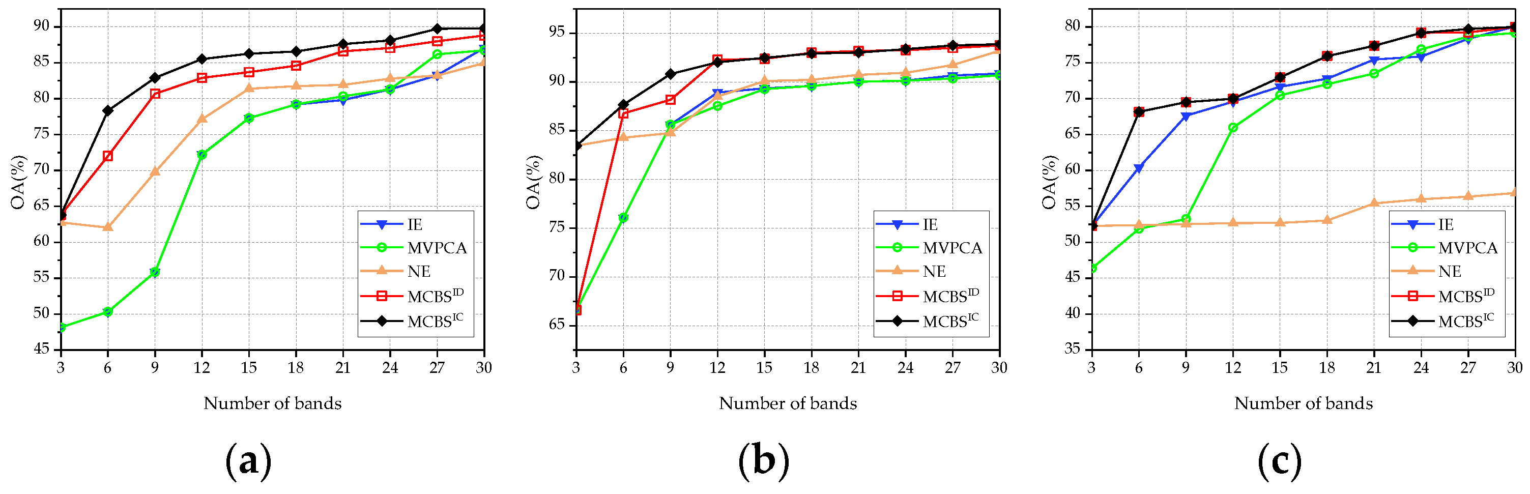
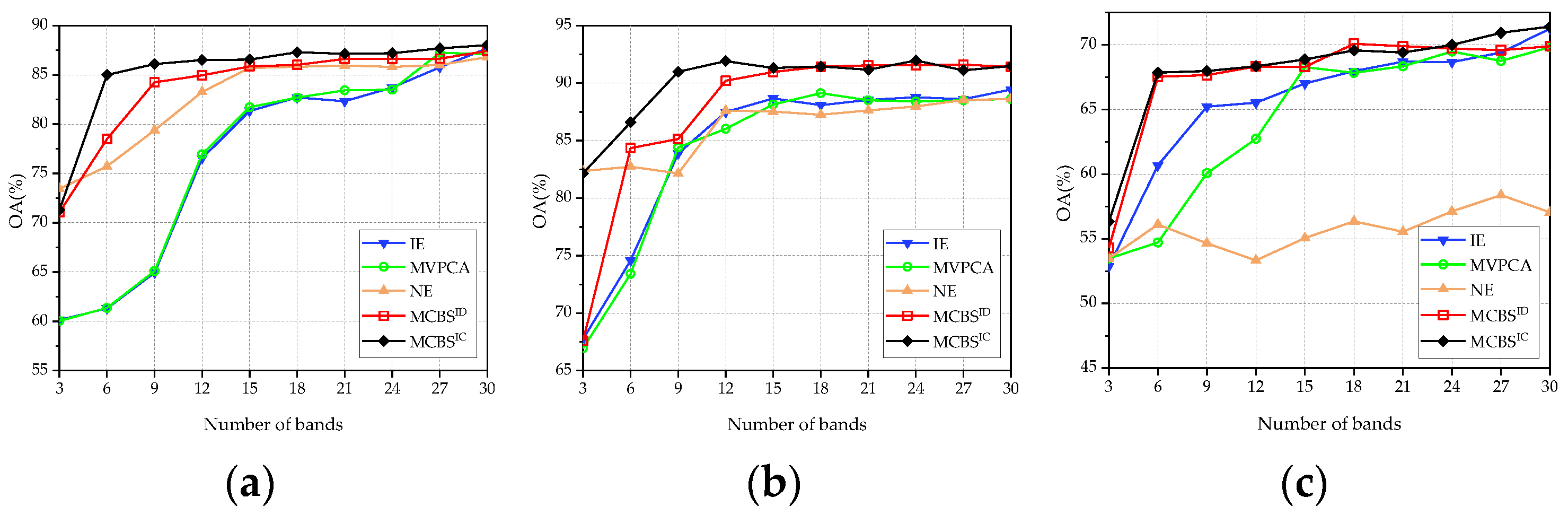
Figure 4 and Figure 5 display the OA curves on three employed data sets produced by SVM and KNN classifiers, respectively. Overall, the OA values of MCBS are significantly higher than its benchmark algorithms. Specifically, the performance of MCBSIC is relatively better than MCBSID due to the consideration of correlation between different criteria. It is also worth noting that when the number of bands is small, the superiority of MCBS is more remarkable. This is because the baseline methods are all single-criterion-based methods. When few bands are selected, the obtained bands are generally extreme ones and even outliers. On the contrary, MCBS integrates multiple criteria to measure the bands, which effectively avoids this problem.
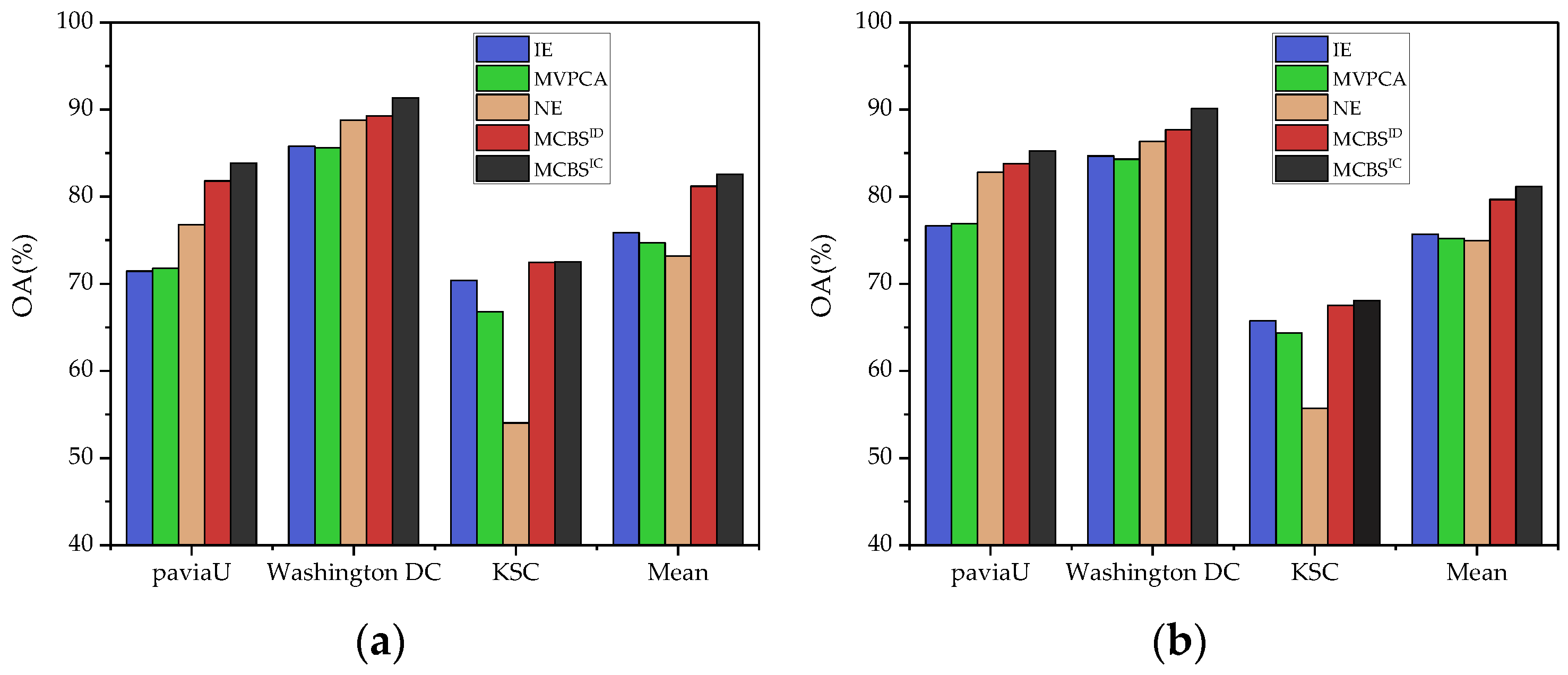
In addition, Figure 6 shows the average accuracies across all band subsets selected by MCBS and its baseline methods. For all employed data sets and classifiers, the two versions of MCBS achieve the highest AOA. In the comparison of the three benchmark algorithms, NE is superior to the other two in both Pavia University and Washington DC Mall data sets but performs very poorly in KSC. This is because the informative bands in the KSC data set are generally polluted by severe salt noises, and NE selects the noise-less bands while ignoring these informative bands. The performance of NE illustrates that the single-criterion-based BS has insufficient generalization ability against different data sets. Figure 6a,b also provide the mean values of AOA over all employed data sets. MCBSID and MCBSIC show obvious superiority over the benchmark algorithms, which demonstrates that they are more robust for diverse data.
3.2.2. Analysis of Weight Estimation
Since the benchmark criteria differ in their capabilities to measure bands, MCBS provides two weight estimation approaches to balance the contributions of different criteria. In reference to the classification performance in last section, this section analyzes whether these two approaches can effectively evaluate the relative importance of each criterion and assign reasonable weights. Table 2 presents the weights estimated by two different versions of MCBS for the benchmark methods.
On the whole, MCBSID effectively assesses the ability of each criterion to discriminate bands. For example, on the Pavia University data set, it attaches the highest weight to NE, while applying similar weights to IE and MVPCA. The results in Figure 4a and Figure 6 validate the reasonableness of doing so, where NE achieves the best performance in the comparison to the three benchmark methods, and the curves of IE and MVPCA are almost the same. Similarly, the three baselines obtained uniform weights on the Washington DC data, and NE obtained the worst weight on the KSC data, both of which are also consistent with their performance in Figure 4b,c.
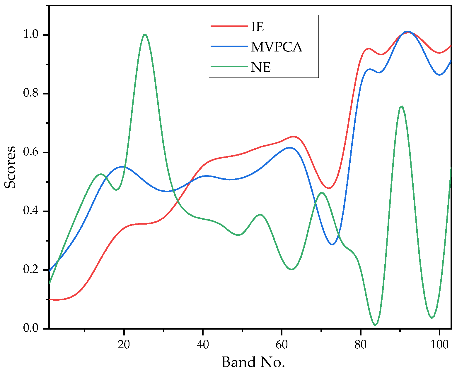
Compared with MCBSID, MCBSIC supplements the consideration of inter-criteria correlation when estimating weights, which is also proved effective in the experimental results. For instance, in Figure 4 and Figure 5, IE and MVPCA perform very similarly at Pavia University, which means that their impact on BS may be redundant. As shown in Figure 7, the distribution curves of their evaluation results are very close. Correspondingly, in Table 2, MCBSIC reduces the weights of these two methods, allowing NE to play a more important role and finally achieve better classification performance than MCBSID.
To sum up, two versions of weight estimation methods in MCBS are demonstrated to be effective, which can objectively make the benchmark criteria trade-off by analyzing the data distribution of the decision matrix. In particular, as an improved version of MCBSID, MCBSIC achieves better performance because it takes into account not only the capability of a criterion to evaluate the bands, but also the inter-relationships between different criteria. Therefore, it is considered preferable in most cases.
3.3. Comparison with State-of-the-Art Methods
In the previous section, the MCBS framework and its weight estimation approaches are proved reasonable. To further investigate the effectiveness and advantages of SP-MCBS, we compare it with some state-of-the-art methods. Besides the baselines, three more sophisticated BS algorithms are employed, including FNGBS [30], E-FDPC [26] and OCF [27]. Among them, OCF has several different implementation versions depending on the employed objective function. Specifically, it introduces two object functions: normalized cut (NC) and top-rank cut (TRC), and three ranking methods: IE, MVPCA, and E-FDPC. Thus, there are six different implementation versions of OCF can be composed, e.g., TRC-OC-FDPC denotes that the TRC and the E-FDPC are utilized. There are two main reasons why we choose TRC-OC-FDPC in the experiments of this paper. On the one hand, based on the results in [27], TRC is more stable than NC. On the other hand, since MCBS also contains both IE and MVPCA ranking functions, we chose E-FDPC for OCF to make it more comparable. Lastly, since the previous section has demonstrated the superiority of IC-based weight estimation, for simplicity, only MCBSIC and SP-MCBSIC are performed in the following experiments.
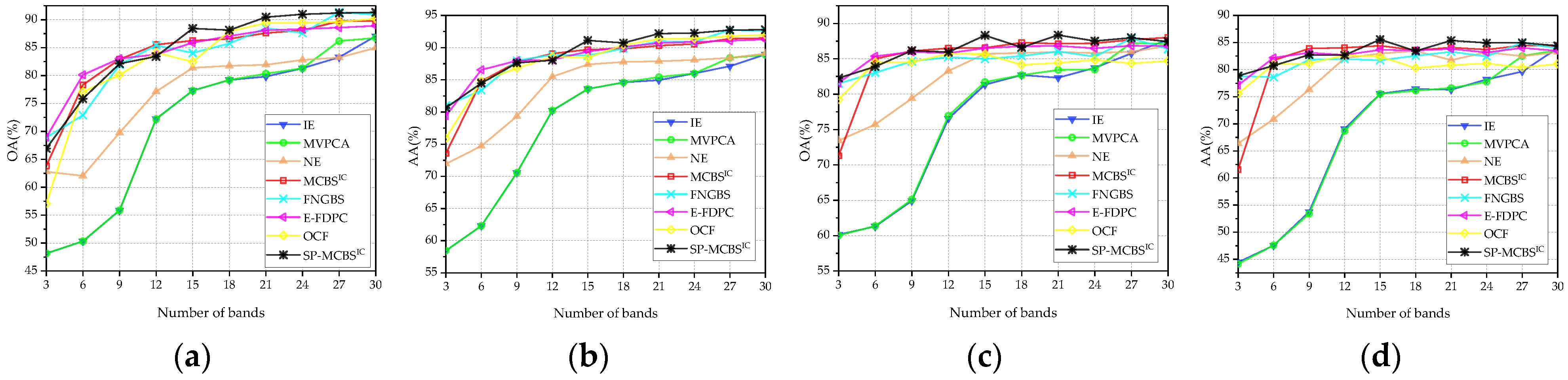
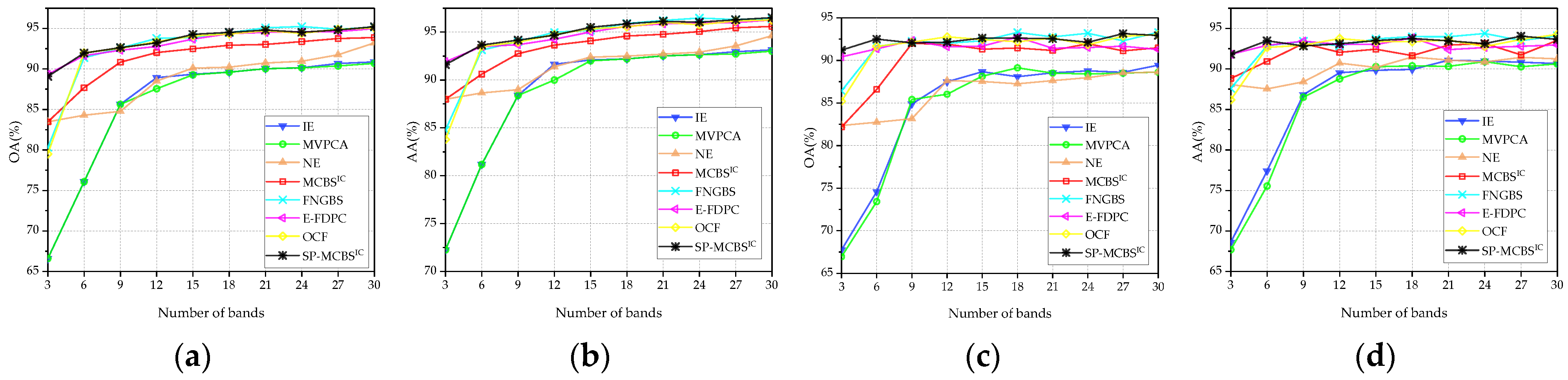
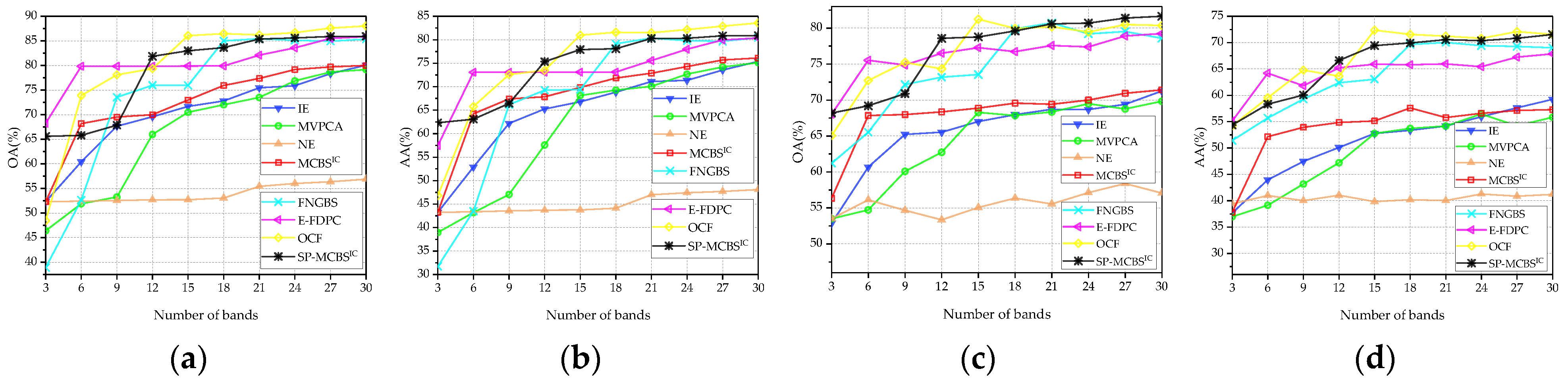
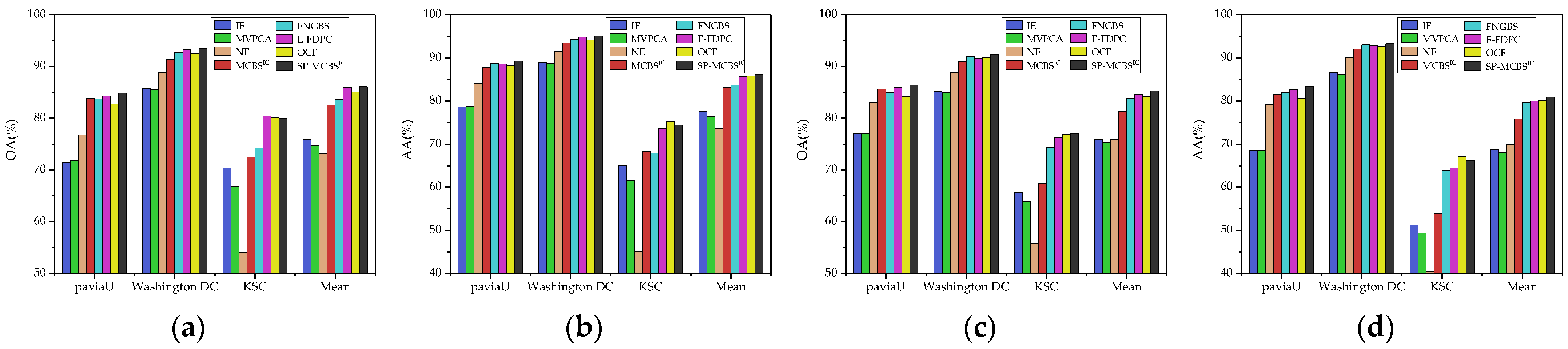
Figure 8, Figure 9 and Figure 10 display the OA and AA curves for the three data sets using the SVM and KNN classifiers. Figure 11 shows the average OA (AOA) and the average AA (AAA) values across the different numbers of bands and provides their mean values over three data sets. In order to further quantitatively compare the classification performance, Table 3 reveals the average of OA and AA calculated by selecting different numbers of bands (the range of 3–30), where the best results are in bold, and the second best are underlined. The quantities after “±” are the standard deviations for ten-times runs of the classifiers under different initial conditions. In addition, Appendix A provides the corresponding classification maps, and the bands selected by different methods are also listed for reference.
(1) Pavia University data set: Figure 8 shows two kinds of indicators on the Pavia University data set. From these panels, it can be observed that SP-MCBSIC outperforms the other methods at some selected bands. Specifically, the performance of MCBS, SP-MCBSIC, FNGBS, E-FDPC and OCF is relatively close to each other, while the three simple ranking-based algorithms, IE, MVPCA and NE, perform obviously worse. When the number of selected bands exceeds 12, MCBSIC show a significant superiority. In addition, as can be seen from Table 3, the proposed method obtains highest values in all four indicators.
(2) Washington DC Mall data set: Figure 9 displays the classification results on the Washington DC Mall data set, the proposed method still achieves competitive performance. In particular, the results are slightly different with respect to classifiers. When SVM is employed, SP-MCBSIC and E-FDPC show stable and excellent performance over the whole range of the number of bands, while FNGBS and OCF perform worse when three bands are selected. However, the performance of E-FDPC gets worse on KNN classifier, where its OA decreases with the number of bands being larger. The proposed method exhibits stability against classifiers. As show in Table 3, SP-MCBSIC obtains the highest average values of OA and AA whether SVM and KNN are used.
(3) KSC data set: Similar to the above two data sets, the classification results of KSC are shown in Figure 10 and Table 3. Due to the KSC data set being seriously polluted by noises, the classification accuracy of all employed methods is degraded. Specifically, E-FPDC shows a relatively stable performance with a small number of bands, while the results of NE are significantly lower than others. This may be because NE inherently assumes a uniform area as part of its calculation and may not be suitable for highly varying scenes. Influenced by NE, the performance of SP-MCBSIC is not as superior as that of the first two data sets. Nevertheless, when the number of bands reaches 12, it outperforms the others on both OA and AA across different classifiers. For the KNN classifier, SP-MCBSIC gets the highest OA among all competitors when the number of bands is 3, 12, 24, 27 or 30.
4. Discussion
According to the experimental results in Sections 3.2 and 3.3, we would like to discuss some interesting issues, and try to give some constructive suggestions for the design of the BS algorithm.
(1) Performance of BS in different implementation modes. The competitors employed in the above experiments can be roughly divided into three categories. The first category is the ranking-based algorithm, including IE, MVPCA and NE. Since being sensitive to extreme bands, they are always unstable when the number of bands is small, as shown in Figure 4 and Figure 5. In addition, the incomprehensive band measurement by a single criterion also results in poor robustness against the data sets, e.g., the performance of NE in Figure 6. The second category is the clustering-based algorithm, such as E-FDPC. In Figure 10, the results of the KSC data set show its superior when selecting a few bands and in its robustness to noises. However, due to some information-rich bands being ignored, it is always difficult to outstand all the competitors. The last category is the SP-based method, which is a combination of the above two categories. The typical methods, such as FNGBS and OCF, first divide all the bands into different subspaces by a given partitioning or clustering strategy, then select bands from each subspace based on various BP criteria. Experimentally, the performance of SP-based methods is significantly improved with the clustering or ranking methods, which is more reasonable for designing an effective BS.
(2) The advantages of MCBS and the reason why SP-MCBS works. According to the experiments in Section 3.2, the main advantages of MCBS over its benchmark methods are its stability with a small number of bands and robustness against data sets. However, although the integration of multiple criteria allows evaluation from additional perspectives, MCBS is still a ranking-based BS that suffers from neglecting band correlation. As a result, SP-MCBS is proposed as an extended version to obtain better performance. In fact, most of the existing SP-based methods are still based on a single criterion, which leads to insufficient band evaluation and insufficient generalization ability for data sets. For example, FNGBS selects one band from each subspace by calculating the product of its local density and entropy. SP-MCBS combines three BP criteria, IE, MVPCA, and NE, and adaptively balances their benefits. Hence, it is expected to obtain a more comprehensive band evaluation and stronger robustness to the data set. Figure 11 confirms the above statements, where SP-MCBS achieves the highest mean values for all four indicators across different data sets.
(3) Drawback of the proposed method. Although the proposed method performs well in the experiments, its performance is still limited by its benchmark methods to some extent. As shown in Figure 10 and Table 3, due to NE exhibiting strong inapplicability to the KSC data, the performance of SP-MCBS is not as superior as that of the other two data sets. In the future, we will focus on two issues to improve the proposed method. One is to choose the baseline algorithms as typical and diverse as possible, so as to evaluate the bands from wider perspectives. Another is to further optimize the weight estimation method, which allows the more appropriate baseline method to obtain higher decision participation.
5. Conclusions
Single-criterion-based BS often leads to insufficient band evaluation. As a result, this work introduces a novel unsupervised BS framework, MCBS, which can effectively combine multiple criteria and select bands from multi-view. Using several typical BPs as the baselines, MCBS constructs a decision matrix to integrate the measurements with different focuses, and then selects bands according to the relative closeness to the global ideal solutions. The weight estimation module adaptively measures the evaluation capability of each criterion and further balance the advantages to maximize their strengths. Another contribution is to provide an extended version of MCBS. This article shows a more sophisticated variant, SP-MCBS, which incorporates CDSP to further reduce the correlation of selected bands. In this paper, HSI classification was chosen as the intended application to validate the effectiveness of BS. Extensive experiments on three public data sets verify that SP-MCBS is more robust against different data sets and outperforms other state-of-the-art methods. Last but not least, MCBS is highly scalable, the employed BP criteria can be replaced as needed to suit different applications. Nevertheless, the selection of appropriate baseline methods is the limitation of our method. However, since it can effectively integrate most existing ranking-based BP, we believe MCBS is very informative for related research topics.
Author Contributions
Conceptualization, X.S. (Xudong Sun) and X.F.; methodology, X.S. (Xudong Sun); software, X.S. (Xin Shen) and H.P.; validation, X.S. (Xudong Sun) and H.P.; formal analysis, X.S. (Xin Shen); writing—original draft preparation, X.S. (Xudong Sun) and X.S. (Xin Shen); writing—review and editing, X.F. and H.P.; visualization, X.S. (Xudong Sun); supervision, X.F. and X.S. (Xudong Sun). All authors have read and agreed to the published version of the manuscript.
Funding
This research was funded by National Natural Science Foundation of China, grant number 62176037 and 62002041; Dalian Science and Technology Innovation Fund, grant number 2018J12GX037, 2019J11CY001 and 2021JJ12GX028; Cultivation Program for the Excellent Doctoral Dissertation of Dalian Maritime University, grant number 2022YBPY008.
Data Availability Statement
The Pavia University and Kennedy Space Center data sets are available online at https://www.ehu.eus/ccwintco/index.php/Sensores-hiperespectrales, accessed on 30 July 2022. And the Washington DC Mall data set is available online at https://rslab.ut.ac.ir/data, accessed on 28 July 2022.
Acknowledgments
The authors would like to thank the editors and the reviewers for their valuable suggestions.
Conflicts of Interest
The authors declare no conflict of interest.
Appendix A
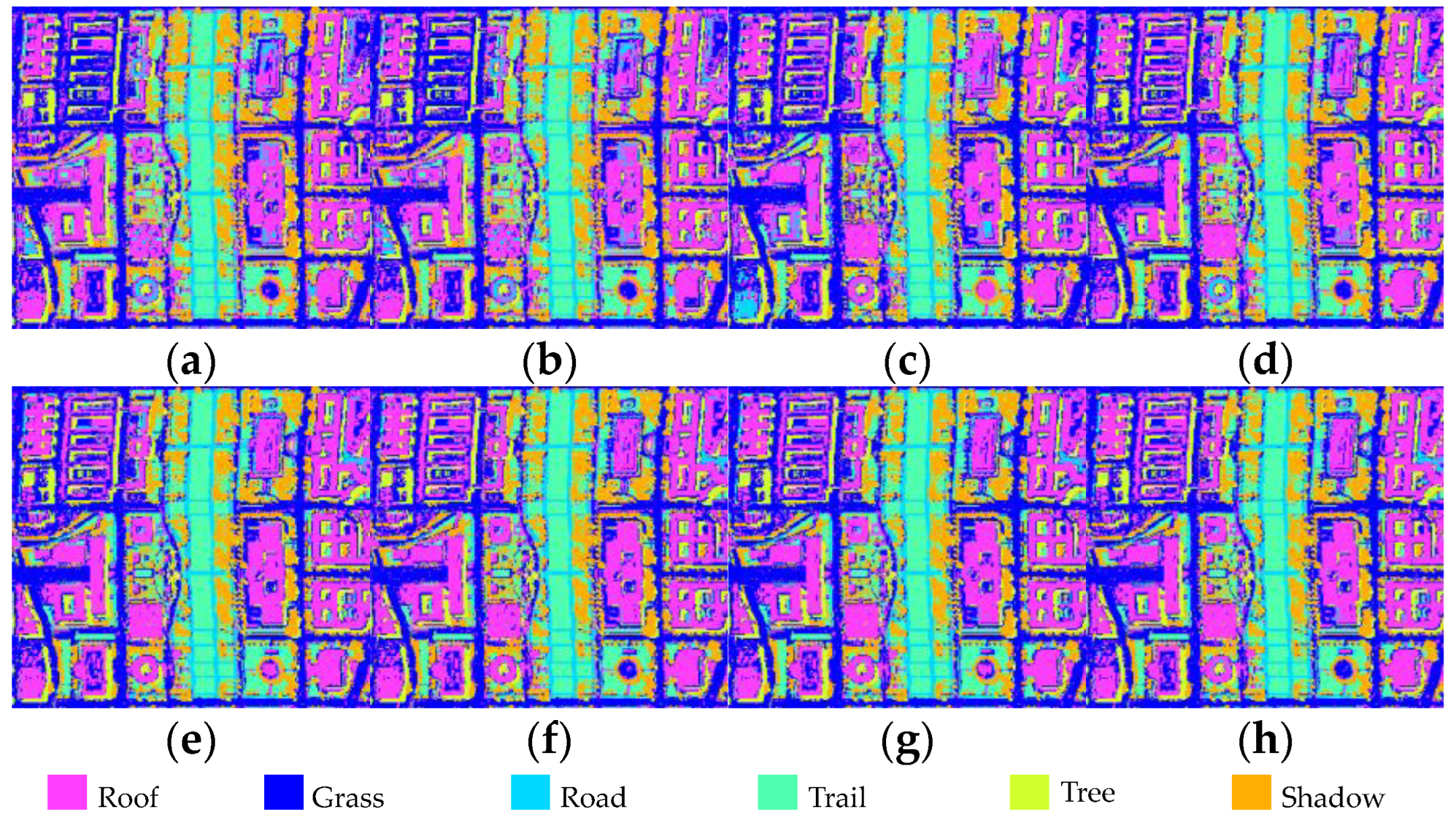
In this section, the classification maps corresponding to Section 3.3 are given to facilitate a visual comparison of the classification performance. For Figure A1, Figure A2 and Figure A3, the number of selected bands are set to 15, 15, 12, respectively. The displayed results are the best ones among 10 executions with the SVM classifier, and their corresponding OA values are also given in parentheses. In addition, Table A1 lists the band subsets selected by the different BS methods for reference.
Figure A1.
Classification maps obtained by different BS methods for Pavia University. The OA values are given in the parentheses (a) IE (77.30%); (b) MVPCA (77.30%) (c) NE (81.38%); (d) MCBSIC (86.26%); (e) FNGBS (84.04%); (f) E-FDPC (85.89%); (g) OCF (82.44%); (h) SP-MCBSIC (88.43%).
Figure A1.
Classification maps obtained by different BS methods for Pavia University. The OA values are given in the parentheses (a) IE (77.30%); (b) MVPCA (77.30%) (c) NE (81.38%); (d) MCBSIC (86.26%); (e) FNGBS (84.04%); (f) E-FDPC (85.89%); (g) OCF (82.44%); (h) SP-MCBSIC (88.43%).

Figure A2.
Classification maps obtained by different BS methods for Washington DC Mall. The OA values are given in the parentheses (a) IE (89.35%); (b) MVPCA (89.27%) (c) NE (90.10%); (d) MCBSIC (92.48%); (e) FNGBS (93.89%); (f) E-FDPC (93.68%); (g) OCF (94.07%); (h) SP-MCBSIC (94.26%).
Figure A2.
Classification maps obtained by different BS methods for Washington DC Mall. The OA values are given in the parentheses (a) IE (89.35%); (b) MVPCA (89.27%) (c) NE (90.10%); (d) MCBSIC (92.48%); (e) FNGBS (93.89%); (f) E-FDPC (93.68%); (g) OCF (94.07%); (h) SP-MCBSIC (94.26%).

Figure A3.
Classification maps obtained by different BS methods for KSC. The OA values are given in the parentheses (a) IE (69.58%); (b) MVPCA (65.98%) (c) NE (52.68%); (d) MCBSIC (69.99%); (e) FNGBS (75.98%); (f) E-FDPC (79.86%); (g) OCF (79.34%); (h) SP-MCBSIC (81.86%).
Figure A3.
Classification maps obtained by different BS methods for KSC. The OA values are given in the parentheses (a) IE (69.58%); (b) MVPCA (65.98%) (c) NE (52.68%); (d) MCBSIC (69.99%); (e) FNGBS (75.98%); (f) E-FDPC (79.86%); (g) OCF (79.34%); (h) SP-MCBSIC (81.86%).


Table A1.
Band subset selected by eight methods on three data sets.
| Datasets | Methods | Band Subset 1 |
|---|---|---|
| Pavia University | IE | 91, 90, 88, 92, 89, 87, 95, 93, 94, 96, 82, 83, 86, 97, 103 |
| MVPCA | 91, 88, 90, 89, 87, 92, 93, 95, 94, 96, 82, 86, 83, 97, 103 | |
| NE | 25, 24, 33, 21, 28, 19, 31, 58, 16, 39, 90, 29, 54, 17, 69 | |
| MCBSIC | 90, 87, 103, 58, 101, 83, 25, 89, 54, 21, 24, 39, 33, 19, 28 | |
| FNGBS | 3, 11, 18, 19, 32, 33, 45, 46, 53, 61, 67, 79, 84, 88, 94 | |
| E-FDPC | 61, 92, 33, 19, 52, 99, 82, 37, 42, 90, 50, 56, 54, 48, 86 | |
| OCF 2 | 61, 88, 33, 19, 53, 48, 29, 99, 36, 15, 65, 8, 80, 72, 3 | |
| SP-MCBSIC | 8, 14, 21, 25, 33, 39, 48, 54, 58, 69, 77, 83, 90, 96, 103 | |
| Washington DC Mall | IE | 81, 82, 80, 79, 83, 78, 84, 94, 77, 95, 70, 112, 113, 93, 71 |
| MVPCA | 81, 82, 80, 79, 83, 78, 94, 84, 77, 95, 112, 93, 70, 113, 111 | |
| NE | 173, 185, 11, 182, 191, 172, 10, 180, 175, 34, 166, 187, 149, 177, 170 | |
| MCBSIC | 173, 185, 11, 182, 34, 191, 172, 81, 10, 82, 149, 80, 175, 180, 79 | |
| FNGBS | 6, 18, 22, 46, 52, 65, 80, 92, 105, 118, 127, 142, 149, 162, 178 | |
| E-FDPC | 179, 48, 63, 152, 119, 25, 80, 96, 128, 112, 123, 95, 99, 141, 68 | |
| OCF | 179, 150, 63, 49, 27, 80, 162, 92, 19, 35, 8, 188, 41, 52, 4 | |
| SP-MCBSIC | 11, 18, 34, 51, 53, 68, 81, 95, 111, 117, 136, 149, 166, 173, 185 | |
| KSC | IE | 51, 50, 52, 49, 53, 48, 54, 47, 56, 55, 46, 57 |
| MVPCA | 133, 174, 51, 50, 1, 52, 49, 176, 53, 54, 55, 56 | |
| NE | 50, 51, 52, 89, 65, 83, 60, 71, 69, 62, 61, 87 | |
| MCBSIC | 50, 51, 52, 72, 67, 68, 53, 49, 54, 56, 55, 74 | |
| FNGBS | 5, 16, 24, 45, 49, 69, 78, 97, 117, 128, 152, 155 | |
| E-FDPC | 65, 53, 22, 9, 66, 81, 82, 87, 84, 86, 89, 96 | |
| OCF | 65, 51, 23, 10, 17, 45, 78, 42, 6, 38, 33, 35 | |
| SP-MCBSIC | 1, 28, 45, 50, 72, 75, 100, 107, 133, 134, 160, 174 |
1 The number of selected bands for three data sets are set in turn to 15, 15, 12. 2 The implementation version of OCF is TRC-OC-FDPC.
References
- Shang, X.; Song, M.; Wang, Y.; Yu, C.; Yu, H.; Li, F.; Chang, C.I. Target-constrained interference-minimized band selection for hyperspectral target detection. IEEE Trans. Geosci. Remote Sens. 2021, 59, 6044–6064. [Google Scholar] [CrossRef]
- Jakob, S.; Zimmermann, R.; Gloaguen, R. The need for accurate geometric and radiometric corrections of drone-borne hyperspectral data for mineral exploration: Mephystoa toolbox for pre-processing drone-borne hyperspectral data. Remote Sens. 2017, 9, 88. [Google Scholar] [CrossRef] [Green Version]
- Pour, A.B.; Park, T.Y.S.; Park, Y.; Hong, J.K.; Zoheir, B.; Pradhan, B.; Ayoobi, I.; Hashim, M. Application of multi-sensor satellite data for exploration of Zn-Pb sulfide mineralization in the Franklinian Basin, North Greenland. Remote Sens. 2018, 10, 1186. [Google Scholar] [CrossRef] [Green Version]
- Bohnenkamp, D.; Behmann, J.; Mahlein, A.K. In-field detection of yellow rust in wheat on the ground canopy and UAV scale. Remote Sens. 2019, 11, 2495. [Google Scholar] [CrossRef] [Green Version]
- Li, Z.Q.; Xie, Y.Q.; Hou, W.Z.; Liu, Z.H.; Bai, Z.G.; Hong, J.; Ma, Y.; Huang, H.L.; Lei, X.F.; Sun, X.B.; et al. In-orbit test of the polarized scanning atmospheric corrector (PSAC) onboard Chinese environmental protection and disaster monitoring satellite constellation HJ-2 A/B. IEEE Trans. Geosci. Remote Sens. 2022, 60, 4108217. [Google Scholar] [CrossRef]
- Wang, Q.; Sun, L.; Wang, Y.; Zhou, M.; Hu, M.H.; Chen, J.G.; Wen, Y.; Li, Q.L. Identification of melanoma from hyperspectral pathology image using 3D convolutional networks. IEEE Trans. Med. Imaging 2021, 40, 218–227. [Google Scholar] [CrossRef]
- Chen, H.M.; Wang, H.C.; Chai, J.W.; Chen, C.C.C.; Xue, B.; Wang, L.; Yu, C.Y.; Wang, Y.L.; Song, M.P.; Chang, C.I. A hyperspectral imaging approach to white matter hyperintensities detection in brain magnetic resonance images. Remote Sens. 2017, 9, 1174. [Google Scholar] [CrossRef] [Green Version]
- Shang, X.D.; Song, M.P.; Wang, Y.L.; Yu, H.Y. Residual-driven band selection for hyperspectral anomaly detection. IEEE Geosci. Remote Sens. Lett. 2022, 19, 6004805. [Google Scholar] [CrossRef]
- Wang, Q.; Zhang, F.H.; Li, X.L. Hyperspectral band selection via optimal neighborhood reconstruction. IEEE Trans. Geosci. Remote Sens. 2020, 58, 8465–8476. [Google Scholar] [CrossRef]
- Chiang, S.S.; Chang, C.I.; Ginsberg, I.W. Unsupervised target detection in hyperspectral images using projection pursuit. IEEE Trans. Geosci. Remote Sens. 2001, 39, 1380–1391. [Google Scholar] [CrossRef]
- Du, Q. Modified fisher’s linear discriminant analysis for hyperspectral imagery. IEEE Geosci. Remote Sens. Lett. 2007, 4, 503–507. [Google Scholar] [CrossRef]
- Fauvel, M.; Chanussot, J.; Benediktsson, J.A. Kernel principal component analysis for the classification of hyperspectral remote sensing data over urban areas. EURASIP J. Adv. Signal Process. 2009, 2009, 783194. [Google Scholar] [CrossRef] [Green Version]
- Li, W.; Prasad, S.; Fowler, J.E.; Bruce, L.M. Locality-preserving dimensionality reduction and classification for hyperspectral image analysis. IEEE Trans. Geosci. Remote Sens. 2012, 50, 1185–1198. [Google Scholar] [CrossRef] [Green Version]
- Li, W.; Prasad, S.; Fowler, J.E. Noise-adjusted subspace discriminant analysis for hyperspectral imagery classification. IEEE Geosci. Remote Sens. Lett. 2013, 10, 1374–1378. [Google Scholar] [CrossRef] [Green Version]
- Roweis, S.T.; Saul, L.K. Nonlinear dimensionality reduction by locally linear embedding. Science 2000, 290, 2323–2326. [Google Scholar] [CrossRef] [PubMed] [Green Version]
- He, X.F.; Niyogi, P. Locality preserving projections. In Advances in Neural Information Processing Systems 16; Bradford: Chester, NJ, USA, 2004; pp. 153–160. [Google Scholar]
- He, X.; Cai, D.; Han, J. Learning a maximum margin subspace for image retrieval. IEEE Trans. Knowl. Data Eng. 2008, 20, 189–201. [Google Scholar] [CrossRef] [Green Version]
- Fu, X.P.; Shang, X.D.; Sun, X.D.; Yu, H.Y.; Song, M.P.; Chang, C.I. Underwater hyperspectral target detection with band selection. Remote Sens. 2020, 12, 1056. [Google Scholar] [CrossRef] [Green Version]
- Li, S.Y.; Peng, B.D.; Fang, L.; Li, Q. Hyperspectral band selection via optimal combination strategy. Remote Sens. 2022, 14, 2858. [Google Scholar] [CrossRef]
- Feng, J.; Jiao, L.C.; Liu, F.; Sun, T.; Zhang, X.R. Mutual-information-based semi-supervised hyperspectral band selection with high discrimination, high information, and low redundancy. IEEE Trans. Geosci. Remote Sens. 2015, 53, 2956–2969. [Google Scholar] [CrossRef]
- Chang, C.I.; Du, Q.; Sun, T.L.; Althouse, M.L.G. A joint band prioritization and band-decorrelation approach to band selection for hyperspectral image classification. IEEE Trans. Geosci. Remote Sens. 1999, 37, 2631–2641. [Google Scholar] [CrossRef]
- Wang, L.; Li, H.C.; Xue, B.; Chang, C.I. Constrained band subset selection for hyperspectral imagery. IEEE Geosci. Remote Sens. Lett. 2017, 14, 2032–2036. [Google Scholar] [CrossRef]
- Su, P.F.; Liu, D.Z.; Li, X.H.; Liu, Z.G. A saliency-based band selection approach for hyperspectral imagery inspired by scale selection. IEEE Geosci. Remote Sens. Lett. 2018, 15, 572–576. [Google Scholar] [CrossRef]
- Ji, H.C.; Zuo, Z.Y.; Han, Q.L. A divisive hierarchical clustering approach to hyperspectral band selection. IEEE Trans. Instrum. Meas. 2022, 71, 1–12. [Google Scholar] [CrossRef]
- Martinez-Uso, A.; Pla, F.; Sotoca, J.M.; Garcia-Sevilla, P. Clustering-based hyperspectral band selection using information measures. IEEE Trans. Geosci. Remote Sens. 2007, 45, 4158–4171. [Google Scholar] [CrossRef]
- Jia, S.; Tang, G.H.; Zhu, J.S.; Li, Q.Q. A novel ranking-based clustering approach for hyperspectral band selection. IEEE Trans. Geosci. Remote Sens. 2016, 54, 88–102. [Google Scholar] [CrossRef]
- Wang, Q.; Zhang, F.H.; Li, X.L. Optimal clustering framework for hyperspectral band selection. IEEE Trans. Geosci. Remote Sens. 2018, 56, 5910–5922. [Google Scholar] [CrossRef] [Green Version]
- Wang, Q.; Li, Q.; Li, X.L. Hyperspectral band selection via adaptive subspace partition strategy. IEEE J. Sel. Top. Appl. Earth Observ. Remote Sens. 2019, 12, 4940–4950. [Google Scholar] [CrossRef]
- Sun, X.D.; Zhang, H.Q.; Xu, F.Q.; Zhu, Y.; Fu, X.P. Constrained-target band selection with subspace partition for hyperspectral target detection. IEEE J. Sel. Top. Appl. Earth Observ. Remote Sens. 2021, 14, 9147–9161. [Google Scholar] [CrossRef]
- Wang, Q.; Li, Q.; Li, X.L. A fast neighborhood grouping method for hyperspectral band selection. IEEE Trans. Geosci. Remote Sens. 2021, 59, 5028–5039. [Google Scholar] [CrossRef]
- Cai, Y.M.; Liu, X.B.; Cai, Z.H. Bs-nets: An end-to-end framework for band selection of hyperspectral image. IEEE Trans. Geosci. Remote Sens. 2020, 58, 1969–1984. [Google Scholar] [CrossRef]
- Dou, Z.Y.; Gao, K.; Zhang, X.D.; Wang, H.; Han, L. Band selection of hyperspectral images using attention-based autoencoders. IEEE Geosci. Remote Sens. Lett. 2021, 18, 147–151. [Google Scholar] [CrossRef]
- Zhang, H.Q.; Sun, X.D.; Zhu, Y.; Xu, F.Q.; Fu, X.P. A global-local spectral weight network based on attention for hyperspectral band selection. IEEE Geosci. Remote Sens. Lett. 2022, 19, 1–5. [Google Scholar] [CrossRef]
- Hu, P.; Liu, X.B.; Cai, Y.M.; Cai, Z.H. Band selection of hyperspectral images using multiobjective optimization-based sparse self-representation. IEEE Geosci. Remote Sens. Lett. 2019, 16, 452–456. [Google Scholar] [CrossRef]
- Sun, W.W.; Jiang, M.; Li, W.Y.; Liu, Y.N. A symmetric sparse representation-based band selection method for hyperspectral imagery classification. Remote Sens. 2016, 8, 238. [Google Scholar] [CrossRef] [Green Version]
- Wang, J.Y.; Wang, H.M.; Ma, Z.Y.; Wang, L.; Wang, Q.; Li, X.L. Unsupervised hyperspectral band selection based on hypergraph spectral clustering. IEEE Geosci. Remote Sens. Lett. 2022, 19, 5509905. [Google Scholar] [CrossRef]
- Das, S.; Pratiher, S.; Kyal, C.; Ghamisi, P. Sparsity regularized deep subspace clustering for multicriterion-based hyperspectral band selection. IEEE J. Sel. Top. Appl. Earth Observ. Remote Sens. 2022, 15, 4264–4278. [Google Scholar] [CrossRef]
- Wang, J.Q.; Lu, P.; Zhang, H.Y.; Chen, X.H. Method of multi-criteria group decision-making based on cloud aggregation operators with linguistic information. Inf. Sci. 2014, 274, 177–191. [Google Scholar] [CrossRef]
- Ren, P.J.; Xu, Z.S.; Gou, X.J. Pythagorean fuzzy TODIM approach to multi-criteria decision making. Appl. Soft. Comput. 2016, 42, 246–259. [Google Scholar] [CrossRef]
- Liu, Y.; Eckert, C.M.; Earl, C. A review of fuzzy AHP methods for decision-making with subjective judgements. Expert Syst. Appl. 2020, 161, 113738. [Google Scholar] [CrossRef]
- Akram, M.; Ilyas, F.; Garg, H. Multi-criteria group decision-making based on ELECTRE I method in Pythagorean fuzzy information. Soft Comput. 2020, 24, 3425–3453. [Google Scholar] [CrossRef]
- Chen, P.Y. Effects of the entropy weight on TOPSIS. Expert Syst. Appl. 2021, 168, 114186. [Google Scholar] [CrossRef]
- Wang, Y.; Hong, H.Y.; Chen, W.; Li, S.J.; Pamucar, D.; Gigovic, L.; Drobnjak, S.; Bui, D.T.; Duan, H.X. A hybrid GIS multi-criteria decision-making method for flood susceptibility mapping at Shangyou, China. Remote Sens. 2019, 11, 62. [Google Scholar] [CrossRef] [Green Version]
- Garg, R. MCDM-based parametric selection of cloud deployment models for an academic organization. IEEE Trans. Cloud Comput. 2022, 10, 863–871. [Google Scholar] [CrossRef]
- Das, R.; Wang, Y.; Putrus, G.; Kotter, R.; Marzband, M.; Herteleer, B.; Warmerdam, J. Multi-objective techno-economic-environmental optimisation of electric vehicle for energy services. Appl. Energy 2020, 257, 113541. [Google Scholar] [CrossRef]
- Adem, A.; Cakit, E.; Dagdeviren, M. Selection of suitable distance education platforms based on human-computer interaction criteria under fuzzy environment. Neural Comput. Appl. 2022, 34, 7919–7931. [Google Scholar] [CrossRef]
Figure 1.
Flowchart of MCBS framework.

Figure 2.
Schematic diagram of CDSP.

Figure 3.
False-color image and ground-truth of the data sets in our experiments. (a) Pavia University; (b) Washington DC Mall; (c) KSC.
Figure 3.
False-color image and ground-truth of the data sets in our experiments. (a) Pavia University; (b) Washington DC Mall; (c) KSC.

Figure 4.
OA curves produced by SVM classifier on different data sets. (a) Pavia University; (b) Washington DC Mall; (c) KSC.
Figure 4.
OA curves produced by SVM classifier on different data sets. (a) Pavia University; (b) Washington DC Mall; (c) KSC.

Figure 5.
OA curves produced by KNN classifier on different data sets. (a) Pavia University; (b) Washington DC Mall; (c) KSC.
Figure 5.
OA curves produced by KNN classifier on different data sets. (a) Pavia University; (b) Washington DC Mall; (c) KSC.

Figure 6.
Average OA values across all band subsets with the band numbers from 3 to 30. (a) results by SVM classifier; (b) results by KNN classifier.
Figure 6.
Average OA values across all band subsets with the band numbers from 3 to 30. (a) results by SVM classifier; (b) results by KNN classifier.

Figure 7.
Distribution of evaluation results obtained by three baseline methods on Pavia University.
Figure 7.
Distribution of evaluation results obtained by three baseline methods on Pavia University.

Figure 8.
OA and AA curves for two classifiers by selecting different numbers of bands on the Pavia University data set. (a) OA by SVM; (b) AA by SVM; (c) OA by KNN; (d) AA by KNN.
Figure 8.
OA and AA curves for two classifiers by selecting different numbers of bands on the Pavia University data set. (a) OA by SVM; (b) AA by SVM; (c) OA by KNN; (d) AA by KNN.

Figure 9.
OA and AA curves for two classifiers by selecting different numbers of bands on Washington DC Mall data set. (a) OA by SVM; (b) AA by SVM; (c) OA by KNN; (d) AA by KNN.
Figure 9.
OA and AA curves for two classifiers by selecting different numbers of bands on Washington DC Mall data set. (a) OA by SVM; (b) AA by SVM; (c) OA by KNN; (d) AA by KNN.

Figure 10.
OA and AA curves for two classifiers by selecting different numbers of bands on KSC data set. (a) OA by SVM; (b) AA by SVM; (c) OA by KNN; (d) AA by KNN.
Figure 10.
OA and AA curves for two classifiers by selecting different numbers of bands on KSC data set. (a) OA by SVM; (b) AA by SVM; (c) OA by KNN; (d) AA by KNN.

Figure 11.
AOA and AAA value on each data set and their mean values over three data sets. (a) OA by SVM; (b) AA by SVM; (c) OA by KNN; (d) AA by KNN.
Figure 11.
AOA and AAA value on each data set and their mean values over three data sets. (a) OA by SVM; (b) AA by SVM; (c) OA by KNN; (d) AA by KNN.

Table 1.
Information of data sets in our experiments.
| Data Sets | Pixels | Wavelength Range | Classes | Bands |
|---|---|---|---|---|
| Pavia University | 610 × 340 | 0.4–2.5 μm | 9 | 103 |
| Washington DC Mall | 280 × 307 | 0.4–2.4 μm | 6 | 191 |
| KSC | 512 × 614 | 0.4–2.5 μm | 13 | 176 |
Table 2.
The weights estimated by two different versions of MCBS for the benchmark methods.
| Weights in MCBSID | Weights in MCBSIC | |||||
|---|---|---|---|---|---|---|
| IE | MVPCA | NE | IE | MVPCA | NE | |
| Pavia University | 0.3170 | 0.3129 | 0.3701 | 0.2227 | 0.2641 | 0.5132 |
| Washington DC Mall | 0.3054 | 0.3543 | 0.3403 | 0.2311 | 0.3177 | 0.4512 |
| KSC | 0.3620 | 0.4309 | 0.2071 | 0.2420 | 0.5420 | 0.2169 |
Table 3.
The average values of OA and AA calculated by selecting different numbers of bands (the range of 3–30 in 3-band intervals), where the best results are in bold and the second-best ones are underlined. The quantities after “±” are the standard deviations for ten-times runs of the classifiers under different initial conditions.
| Datasets | Classifier (Measure) | IE | MVPCA | NE | MCBSIC | FNGBS | E-FDPC | OCF 1 | SP-MCBSIC |
|---|---|---|---|---|---|---|---|---|---|
| Pavia University | SVM (OA) | 71.45 ± 0.14 | 71.76 ± 0.15 | 76.77 ± 0.09 | 83.87 ± 0.08 | 83.74 ± 0.07 | 84.28 ± 0.06 | 82.74 ± 0.10 | 84.88 ± 0.08 |
| SVM (AA) | 78.67 ± 0.11 | 78.84 ± 0.11 | 84.01 ± 0.06 | 87.84 ± 0.05 | 88.71 ± 0.04 | 88.55 ± 0.04 | 88.16 ± 0.05 | 89.26 ± 0.04 | |
| KNN (OA) | 76.96 ± 0.10 | 77.05 ± 0.10 | 83.06 ± 0.05 | 85.60 ± 0.05 | 85.04 ± 0.02 | 85.89 ± 0.02 | 84.21 ± 0.02 | 86.44 ± 0.02 | |
| KNN (AA) | 68.48 ± 0.14 | 68.6 ± 0.15 | 79.27 ± 0.06 | 81.59 ± 0.07 | 82.02 ± 0.02 | 82.69 ± 0.02 | 80.66 ± 0.02 | 83.37 ± 0.02 | |
| Washington DC Mall | SVM (OA) | 85.79 ± 0.08 | 85.59 ± 0.08 | 88.80 ± 0.03 | 91.34 ± 0.03 | 92.67 ± 0.05 | 93.27 ± 0.02 | 92.48 ± 0.05 | 93.50 ± 0.02 |
| SVM (AA) | 88.90 ± 0.07 | 88.69 ± 0.07 | 91.57 ± 0.02 | 93.45 ± 0.02 | 94.33 ± 0.04 | 94.80 ± 0.01 | 94.11 ± 0.04 | 95.04 ± 0.02 | |
| KNN (OA) | 85.12 ± 0.08 | 84.93 ± 0.08 | 88.85 ± 0.02 | 90.89 ± 0.02 | 91.94 ± 0.02 | 91.60 ± 0.01 | 91.67 ± 0.02 | 92.39 ± 0.01 | |
| KNN (AA) | 86.57 ± 0.08 | 86.12 ± 0.08 | 90.09 ± 0.02 | 92.03 ± 0.01 | 93.03 ± 0.02 | 92.88 ± 0.01 | 92.64 ± 0.02 | 93.27 ± 0.01 | |
| KSC | SVM (OA) | 70.41 ± 0.09 | 66.82 ± 0.12 | 54.03 ± 0.02 | 72.51 ± 0.08 | 74.28 ± 0.16 | 80.46 ± 0.05 | 80.08 ± 0.12 | 79.93 ± 0.09 |
| SVM (AA) | 65.06 ± 0.10 | 61.62 ± 0.14 | 45.18 ± 0.02 | 68.34 ± 0.10 | 67.94 ± 0.17 | 73.68 ± 0.06 | 75.14 ± 0.12 | 74.41 ± 0.07 | |
| KNN (OA) | 65.65 ± 0.06 | 63.96 ± 0.07 | 55.74 ± 0.01 | 67.35 ± 0.05 | 74.35 ± 0.07 | 76.21 ± 0.03 | 76.90 ± 0.05 | 76.96 ± 0.05 | |
| KNN (AA) | 51.23 ± 0.07 | 49.36 ± 0.07 | 40.47 ± 0.01 | 53.82 ± 0.06 | 63.93 ± 0.07 | 64.46 ± 0.04 | 67.18 ± 0.06 | 66.20 ± 0.06 |
1 The implementation version of OCF is TRC-OC-FDPC.
Publisher’s Note: MDPI stays neutral with regard to jurisdictional claims in published maps and institutional affiliations. |
© 2022 by the authors. Licensee MDPI, Basel, Switzerland. This article is an open access article distributed under the terms and conditions of the Creative Commons Attribution (CC BY) license (https://creativecommons.org/licenses/by/4.0/).
Share and Cite
MDPI and ACS Style
Sun, X.; Shen, X.; Pang, H.; Fu, X. Multiple Band Prioritization Criteria-Based Band Selection for Hyperspectral Imagery. Remote Sens. 2022, 14, 5679. https://doi.org/10.3390/rs14225679
AMA Style
Sun X, Shen X, Pang H, Fu X. Multiple Band Prioritization Criteria-Based Band Selection for Hyperspectral Imagery. Remote Sensing. 2022; 14(22):5679. https://doi.org/10.3390/rs14225679
Chicago/Turabian StyleSun, Xudong, Xin Shen, Huijuan Pang, and Xianping Fu. 2022. "Multiple Band Prioritization Criteria-Based Band Selection for Hyperspectral Imagery" Remote Sensing 14, no. 22: 5679. https://doi.org/10.3390/rs14225679
Note that from the first issue of 2016, this journal uses article numbers instead of page numbers. See further details here.