


The Time Lag Effect Improves Prediction of the Effects of Climate Change on Vegetation Growth in Southwest China


1
Chaozhou Environmental Information Center, Chaozhou 521011, China
2
Department of Renewable Resources, University of Alberta, Edmonton, AB T6G 2E3, Canada
3
School of Life Science and Engineering, Handan University, Handan 056005, China
*
Author to whom correspondence should be addressed.
Remote Sens. 2022, 14(21), 5580; https://doi.org/10.3390/rs14215580
Submission received: 14 September 2022
/
Revised: 29 October 2022
/
Accepted: 1 November 2022
/
Published: 4 November 2022
(This article belongs to the Special Issue Geostatistics and Spatial Data Mining for Ecological Climatology)
Abstract
:Climate change is known to significantly affect vegetation development in the terrestrial system. Because Southwest China (SW) is affected by westerly winds and the South and East Asian monsoon, its climates are complex and changeable, and the time lag effect of the vegetation’s response to the climate has been rarely considered, making it difficult to establish a link between the SW region’s climate variables and changes in vegetation growth rate. This study revealed the characteristics of the time lag reaction and the phased changes in the response of vegetation to climate change across the entire SW and the typical climate type core area (CA) using the moving average method and multiple linear model based on the climatic information of CRU TS v. 4.02 from 1982 to 2017 together with the annual maximum (P100), upper quarter quantile (P75), median (P50), lower quarter quantile (P25), minimum (P5), and mean (Mean) from GIMMS NDVI. Generally, under the single and combined effects of temperature and precipitation, taking the time lag effect (annual and interannual delay effect) into account significantly improved the average prediction rates of temperature and precipitation, which increased by 18.48% and 25.32%, respectively. The optimal time delay was 0–4 months when the annual delay was taken into consideration, but it differed when considering the interannual delay, and the delaying effect of precipitation was more significant than that of temperature. Additionally, the response intensity of vegetation to temperature, precipitation, and their interaction was significantly more robust when the annual delay was taken into account than when it was not (p < 0.05), with corresponding multiple correlation coefficients of 0.87 and 0.91, respectively. However, the degree of response to the combined effect of individual effects and climate factors tended to decrease regardless of whether time delay effects were taken into account. A more comprehensive analysis of the effects of climate change on vegetation development dynamics suggested that the best period for synthesizing NDVI annual values might be the P25 period. Our study could provide a new theoretical framework for analyzing, predicting, and evaluating the dynamic response of vegetation growth to climate change.
1. Introduction
Climate change can significantly affect vegetation development and plays a decisive part in its growth. The response of vegetation to climate conditions has become a hot topic at regional and even global scales, and the connection between vegetation and climate against the background trend of global warming has significant theoretical research value [1,2,3,4,5]. Vegetation development is mainly influenced by temperature and precipitation and is closely related to hydrothermal conditions, making it an ideal choice for considering the relationship between climate and vegetation change [6,7,8,9,10]. In addition, because of the different demands for hydrothermal conditions at each life cycle stage of vegetation growth, the impact of climate factors on vegetation is variable and changes with the interaction of different spatial patterns and time delay effects [11,12,13,14,15,16]. When the amplitude of climate change exceeds the tolerance limit of vegetation growth in a particular month, vegetation will respond differently to climate change [17]. For example, in European beech saplings, the effect of temperature on leaf senescence in autumn was greater than that on deciduous leaves in spring [18]. Furthermore, climate change could directly or indirectly induce and disturb the ecosystem by changing the chemical and physical properties of soil—for example, by increasing temperature, reducing the availability of soil water, and promoting the availability of nitrogen, phosphorus, potassium, and other nutrient elements [19,20]. This has an indirect impact on vegetation development and means that the reaction of vegetation change to meteorological factors has a specific delayed interaction [11]; that is, there is a time lag effect [13,14,16,21,22,23].
Many studies have shown that utilizing the time lag effect could effectively improve the prediction rate for climate impacts on vegetation development at the global scale within the annual cycle, including the developing period, the aging stage, and the complete development season [11,12,14,15,16]. For example, Wu et al. [11] revealed that the clarification rate of climate variables for worldwide changes in vegetation development increased by about 11% and the explanation rate reached 64% when the time lag effect was taken into consideration. Zhao et al. [12] pointed out that when the time lag effect was considered within the Amazon Basin, the explanation rate increased by about 12% to about 40%. Ding et al. [14] indicated that on a global scale, the explanation rate increased by about 15%, 19%, and 17% in the developing period, the aging stage, and the complete development season, respectively. Zhao et al. [16] pointed out that the climatic factors (precipitation and temperature) increased by more than 95% relative to the typical watershed on the Loess Plateau when the time lag was taken into consideration. In the Xijiang River Basin in southern China, the areas where vegetation has been significantly affected by rainfall and temperature exceed 30% of the total basin after accounting for the delay effect [15]. In addition, the length of the delaying effect of climate factors on vegetation varies greatly globally. In low-latitude regions, the delaying effect of temperature on vegetation was more than one month; in the middle- and high-latitude regions, it was generally less than one month [11]; and in the Northern Hemisphere (>30°N), the autumn leaf senescence and drought displayed a lag period of 2–6 months [24]. The lag time of the response of vegetation to climate variables in Northern Eurasia [25] was about 3 months, and in the Qinghai–Xizang Plateau region [26], it was generally 1–4 months. However, the reaction of vegetation to climate variables is not synchronous; for example, in the Red River Basin in southern China [27] and in Ethiopia [22], the reaction of NDVI to temperature was faster than it was to precipitation, and the extreme alpine region of southern Xizang [28] was more sensitive to precipitation than temperature. Similarly, some researchers found that vegetation developed in the southwestern United States [29], inland Australia [21], the Yun–Gui Plateau [30], and Inner Mongolia [31] were unequivocally positively connected with precipitation one month before.
Current research has widely proved the connection between climate and vegetation at both regional and global scales. However, most of these studies considered only the annual cycle and utilized only a maximum or average value of NDVI to establish the annual growth. In reality, in the many growth stages in the life cycle of vegetation, the heat and moisture required are variable, and because of global climate change, there are obvious regional differences, change trends, and volatility, which make research findings inconsistent, complex, and difficult to interpret quantitively; as a result, the explanation rate of climatic factors to vegetation growth is low. Consequently, we posed the following scientific questions: (1) How should we characterize the time delay effect of individual and multiple climatic factors on vegetation and select the optimal time delay? (2) How can we determine the strength variation trend of the delay effect in relation to the response of vegetation to climate factors?
2. Materials and Methods
Therefore, based on the core areas screened out by Wang and An [32], the annual values of maximum (P100), upper quarter quantile (P75), median (P50), lower quarter quantile (P25), minimum (P5), and mean (Mean) of GIMMS NDVI were selected to represent the development status of vegetation at different growth stages. These were used alone and in combination to analyze the time lag’s impact of temperature and precipitation factors and identify the optimal time lag when individual and joint action had a significant impact on NDVI. The response characteristics and periodic change trends in the reaction of vegetation to climate factors (temperature and precipitation, separately and jointly) were analyzed to help us to predict and evaluate the dynamic response of vegetation to worldwide climate change and to provide a theoretical basis for the wider study of global climate change.
2.1. Overview of the Research Area
In accordance with the concept of natural regionalization [33], the “Southwest Region of China” in this study has a broader geographical meaning and takes into account vegetation and landscape settings between the coordinates 21.14°–36.48°N and 83.87°–110.19°E, which cover the Himalayan mountains, the eastern Qinghai–Xizang Plateau, the Hengduan Mountains, the Yun–Gui Plateau, the Sichuan Basin, and other terrain units (Figure 1a) [34]. The entire study area spanned Sichuan, Chongqing, Guizhou, Yunnan, Eastern Xizang, and southern Qinghai. Combined with the unique climatic characteristics of the Qinghai–Xizang Plateau, this area has a critical effect on East Asian and worldwide climate [16,35] and has become an area of significant interest to domestic and foreign scholars [32,34,35].
2.2. Acquisition and Analysis of Research Data
2.2.1. Data Sources and Processing
(1) A digital elevation model (DEM) with a resolution of 1 km obtained from the Resource and Environmental Science and Data Center (as shown in Table 1) was used to characterize the topography of the SW (Figure 1a). Then, the bilinear interpolation extrapolation method was used in ArcGIS10.6 to resample the raster data with a resolution of 0.25° × 0.25°.
(2) Using the resource environment cloud platform (as shown in Table 1) to obtain China’s vegetation zoning data, the SW was divided into six main subregions (Figure 1b).
(3) A high-resolution gridded climatic variables dataset (CRU_TS4. 02) with a determination of 0.5° × 0.5° [36] was obtained from the Climate Research Unit, University of East Anglia, UK (as shown in Table 1). This has been regularly utilized as reliable climate information for the study of global or regional climate changes and the impacts on biological systems (e.g., Buermann et al. [37]; Wang et al. [34]; Wang and An [32]). According to Wang’s research [34], the region’s average temperature and annual precipitation from 1901 to 2017 showed significant inflection points in 1954 and 1928, respectively, and other relevant reports pointed out that the temperature in the Northern Hemisphere began to rise in the mid-1970s, and in particular after 1980 [38,39]. Combined with the longest NDVI time sequence (GIMMS NDVI3g) [40], we selected the period from 1982 to 2017 for our preliminary inquiry.
Because the SW extends across three topographic zones from west to east, with areas of fragmented transition between adjacent zones and a wide range of altitudes, there are significant climate characteristics at different altitudes (such as elevation-dependent warming [41], elevation-dependent wetting [42], etc.). As a result, the 0.5° × 0.5° spatial resolution meteorological data could obscure the subtle relationship between climate change and the environment. Therefore, this study used the cubic spline method [43] to interpolate climate data with a spatial resolution of 0.5° × 0.5° and downscale the resolution to 0.25° × 0.25°.
(4) The NDVI information was selected from the Global Inventory Monitoring and Modeling Studies (GIMMS) dataset from January 1982 to December 2015 (as shown in Table 1) with a time step of 15 d and a spatial grid of 8 km. Although this dataset has been widely used to study vegetation dynamics at global and regional levels after geometric correction, radiometric correction, and atmospheric correction [40], because of the high frequency of clouds and precipitation in the SW, we combined it with Savitzky–Golay filtering [44] to reconstruct the sequence and eliminate cloud interference and used the maximum-value composite method (MVC) [32,34,39] to eliminate interference from cloud, atmosphere, rain, and the altitude of the sun.
In addition, because cultivated vegetation is frequently affected by human activity, such areas needed to be excluded from the analysis in order to focus on the relationship between climate change and natural vegetation growth. In addition, the rapid urbanization of the study area due to the implementation of the Strategy for Large-Scale Development of Western China in around 2000 led to a rapid increase in the number of impervious areas, which also needed to be excluded from the analysis. Therefore, the area of cultivated vegetation obtained from the Resource and Environmental Science and Data Center and the artificial impervious area obtained from the Global Artificial Impervious Area (as shown in Table 1) [45] from the Tsinghua University data open platform were excluded from this study.
To comprehensively display the changing vegetation trends, in accordance with the method described by Wang and An [32], the annual maximum (P100), upper quarter quantile (P75), median (P50), lower quarter quantile (P25), minimum (P5), and mean (Mean) of GIMMSNDVI were chosen to represent the annual diverse development stages of vegetation.
(5) The topographic, climatic, vegetation, and ecoregion distribution data for the study area were obtained from publicly available sources. To ensure scale consistency, they were resampled or reduced to 0.25° × 0.25° raster data to meet the requirements of this study.
2.2.2. Research Methods
(1) Trend analysis and detection: The least square method was utilized for examining the trend of a specific factor, and the trend of the fair condition was used to indicate the change intensity of the factor [34,42]. The formula was:
where n is the research phase and is the factor number of the th year. When > 0, it indicates an expanding drift within the investigated phase; otherwise, it indicates a diminishing drift. The T-test was utilized to test the importance of the changing trend of this factor.
(2) Moving average method: The moving average method was utilized to remove the effect of information interference and reduce the effect of irregular impacts and thus achieve a generally smoother time arrangement that would more intuitively represent the changing trend [46]. The moving average formula was:
where L = 15 years is the sliding step according to the research results of Fu et al. [47], i is the sequence number, and .
(3) Time delay effect of vegetation on individual climatic variables: In order to determine the time delay impact of climate variables on the six annual characteristic values, the month with the highest frequency of characteristic values (except the Mean) in all windows was selected as the month with occurrence of the annual characteristic values, and the month closest to the Mean was defined as the month of Mean occurrence (see Appendix A for details).
The monthly temperature and precipitation data were utilized as independent variables, and six annual synthetic data from GIMMS NDVI (P100, P75, P50, P25, P5, and Mean) were successively taken as response variables to calculate the delay effect of synthetic data with different annual values. Previous studies found that the time lag impact of climate factors on vegetation was, for the most part, less than four months [11,19], and a 2-year time lag impact was also found [48]. Considering that P25 or P5 may occur in January or December of the current year, we selected the current and previous year’s monthly temperature and precipitation data as independent variables. The formula model of NDVI and temperature and precipitation was as follows:
where NDVI is the response variable and is the synthetic data of the annual values of NDVI (P100, P75, P50, P25, P5, and Mean, respectively); represents the regression coefficient of climate factors within the th month, with ranging from 1 to 24, where 1–12 represent months 1–12 of the previous year and 13–24 represent months 1–12 of the current year, respectively; TMP and PRE correspond to time arrangement information of temperature and precipitation in the -th month; is the constant term of the regression model; and is the random error term. NDVI, TMP, and PRE were averaged over a sliding 15-year period before being entered into Equations (3) and (4).
The optimal time delay selection rule: Firstly, in this study, the occurrence month of synthetic data of NDVI annual value is defined as the month with the highest occurrence frequency and is represented by n (1≤ n ≤24) in the new series formed after 15 years of sliding [47], in which the occurrence frequency of Mean is defined as the occurrence frequency of the month with the smallest error with Mean. In the reaction of vegetation to a single climate factor, the th month with the most significant assurance coefficient R2 is selected, which is the ideal time delay. Additionally, cannot exceed the month n in which the synthetic data of six NDVI annual values appear. If this restriction condition is not considered, the eigenvalues may have the largest coefficient of determination with respect to the climatic factor after the month of occurrence, which is clearly against the objective law. The calculation formula of the maximum determination coefficient R2 is:
where is the maximum lag determination coefficient; is the th month; are determinant coefficients of January of the previous year, February of the previous year, and so on, respectively, and n in the same month; and the maximum value is selected from those determinant coefficients as the optimal lag-determining coefficient. If , the optimal lag of NDVI to this climate factor is n − 1 months, and so on; if , the optimal lag is 0 months—that is, there is a maximum determination coefficient in the same month.
(4) Vegetation responses to a combined model of multiple climate factors with multiple time delays: The multiple linear regression model is simple in form and makes it easy to estimate and test parameters which can effectively explore the collective impact of temperature and precipitation on NDVI multiple delays. The multiple time delay combination models are as follows:
where NDVI is the response variable and the synthetic data of the six annual values (P100, P75, P50, P25, P5, and Mean, respectively); and are the regression coefficients of independent variables TMP and PRE in the th and th months, respectively, with and ranging from 1 to 24, where 1–12 represent months 1–12 of the previous year, respectively, and 13–24 represent months 1–12 of the current year, respectively; TMP and PRE correspond to time sequence information on temperature and precipitation in the th and th months, respectively; is the constant term of the regression model; and is the random error term. NDVI, TMP, and PRE were averaged over a sliding 15-year period before being entered into Equation (6).
The optimal time delay selection rule is as follows: In this case, the rule is similar to the optimal time delay selection rule for the delay effect on vegetation of a single climate factor. Specifically, in the response of vegetation to the combined model (the maximum number of 24 × 24 = 576) with multiple delays of temperature and precipitation, the th and th months with the maximum determination coefficient R2—that is, the optimal time delay—are selected. In addition, and should not exceed the month n in which the synthetic data of six NDVI annual values appear. If the restriction condition was not considered, the eigenvalues may have the largest coefficient of determination with respect to the climatic factor after the month of occurrence, which is clearly against the objective law. The calculation formula of the maximum determination coefficient R2 is:
where is the maximum lag determination coefficient; and are the th and th months, respectively; are determinant coefficients of January of the previous year, the temperature in January and the precipitation in February of the previous year, and n in the same month, respectively; and the maximum value is selected from those determinant coefficients as the optimal lag-determining coefficient. If , the optimal lag for both temperature and precipitation factors in NDVI is n − 1 months, and so on; if , the optimal lag is 0 months—that is, there is a maximum determination coefficient in the same month.
(5) The strength of the delay effect in the vegetation response to climate factors: Partial and complex correlation coefficients were utilized to characterize the individual and combined intensity of the vegetation response to temperature and precipitation in completely different months. According to Formula (9), monthly temperature (precipitation) data were fixed, and a partial correlation between precipitation (temperature) and six annual data of GIMMS NDVI (P100, P75, P50, P25, P5, and Mean) was calculated. The multiple relationships between NDVI, temperature, and precipitation were calculated according to Formula (10).
Here, represents the correlation coefficient of the x and y factors; , and , represent climate variable and NDVI in the th year and the multi-year average, respectively; n is the research phase; represents the partial correlation coefficient between x and y when z is fixed, and the T-test was utilized to test the importance; and represents the multiple correlation coefficient between x and y and z, and the F-test was utilized to test the importance. x, y, and z were averaged over a sliding 15-year period before being entered into Equations (8), (9), and (10).
Formulas (11) and (12) are used to calculate the optimal intensity of the time delay response of vegetation to climate factors singly and in combination:
where and represent the maximum absolute value of partial correlation coefficient () and complex correlation coefficient (), respectively, with time delay; is the th month; and are the and of January of the previous year, February of the previous year (and so on), and n in the same month, respectively; and the maximum value is selected from these partial or complex correlation coefficients as the optimal lag correlation coefficient. It is important to note here that if and , then the intensities of x and y are negative and the time lag effect of the final response intensity is of size .
(6) The strength of the variation in the delay effect trend of vegetation response to climate factors: We took every 15 years as a period and calculated the and in this period by combining Equations (8)–(12). In addition, combined with the particular interpretation of step (5), we revealed the response intensity for each period. Then, the response intensities for 1982–1996, 1983–1997, and 2001–2015 were calculated separately, the sequence reconstructed, and the variation tendency calculated in accordance with Equation (1), which referred to the variation tendency of response intensity of vegetation to climatic variables and the importance test using the T-test method.
3. Results
3.1. Time Delay Effect of Climatic Factors on Vegetation
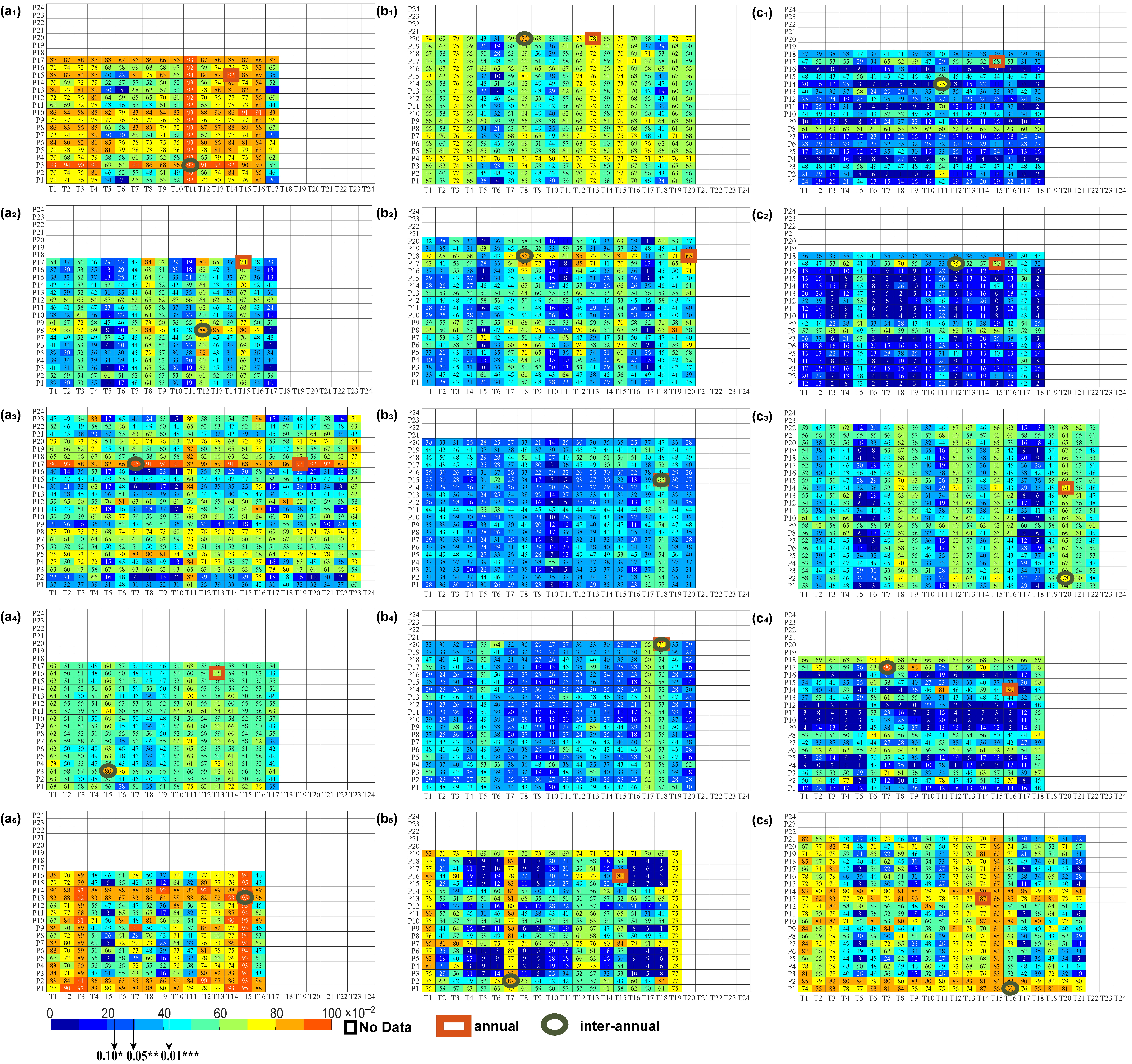
When time delay effects (annual and interannual time delays) were considered, the temperature and precipitation factors and their combined effects significantly improved the prediction rate for vegetation growth compared to the same period (p < 0.05) (Figure 2 and Figure 3). With regard to the annual time delay, the corresponding optimal R2 with the annual time delay increased by 0.02 (3.44%)–0.43 (173.06%), 0.06 (9.75%)–0.31 (80.61%) and 0.07 (9.99%)–0.48 (190.04%), respectively (the percentage in brackets indicates the relative increase in percentage, and this is repeated below). The corresponding optimal R2 of the interannual time delay was further improved by 0.07 (9.99%)–0.48 (190.04%), 0.15 (25.02%)–0.37 (147.34%), and 0.15 (25.02%)–0.37 (147.34%), respectively. Based on the comprehensive results, it was further found that the maximum or submaximum prediction rate exists in the P25 period at the same time, and taking the time delay effect into consideration, the difference between the submaximum and the maximum was less than 0.04, which was higher than the prediction rate in the P100 period. Taking the annual time delay into consideration, the optimal time delay relating to temperature, precipitation and the interaction between them was generally less than or equal to four months, consisting of about 0.40 ± 0.55–3.80 ± 2.59 months for temperature alone and 0.20 ± 0.45–3.80 ± 3.35 months for precipitation alone. The occurrence months of the maximum prediction rate of NDVI by both temperature and precipitation climatic factors were concentrated in the 13–17 months (90%), 18–20 months (60%), 13–17 months (90%), 15–19 months (80%), 13–16 months (100%), and 13–16 months (100%) ranges (the percentages in brackets indicate the frequency of occurrence of the month in which the maximum explanatory rates for temperature and precipitation occur). When at Mean, P100, and P5, the annual optimal time delay months for temperature (∆tannual-T) were more significant than those for precipitation (∆tannual-P), and at P75–P5, ∆tannual-T < ∆tannual-P, the optimal time lag was within the range of one month. Furthermore, it was also found that the optimal time delay for temperature of P100 in SW, P100 in T+*-P+*, P50 in T+*-P−, P50 in T+*-P+, and P75 in NSC was more than four months, and the optimal time delay for precipitation of P50 in SW, P100 in T+*-P+*, Mean in T+*-P−, and P75 in NSC was over four months. With regard to interannual delay, the maximum R2 had a significant difference in the number of optimal delay months, and when temperature and precipitation act together at P100–P50, the interannual time optimal delay months for temperature (∆tinter-annual-T) were more significant than those for precipitation (∆tinter-annual-P). At Mean, P25, and P5, ∆tinter-annual-T < ∆tinter-annual-P and the average optimal delay differed by 1.2, 8.0 and 5.8 months, respectively.
3.2. The Intensity of the Delay Effect of Climate Factors on Vegetation
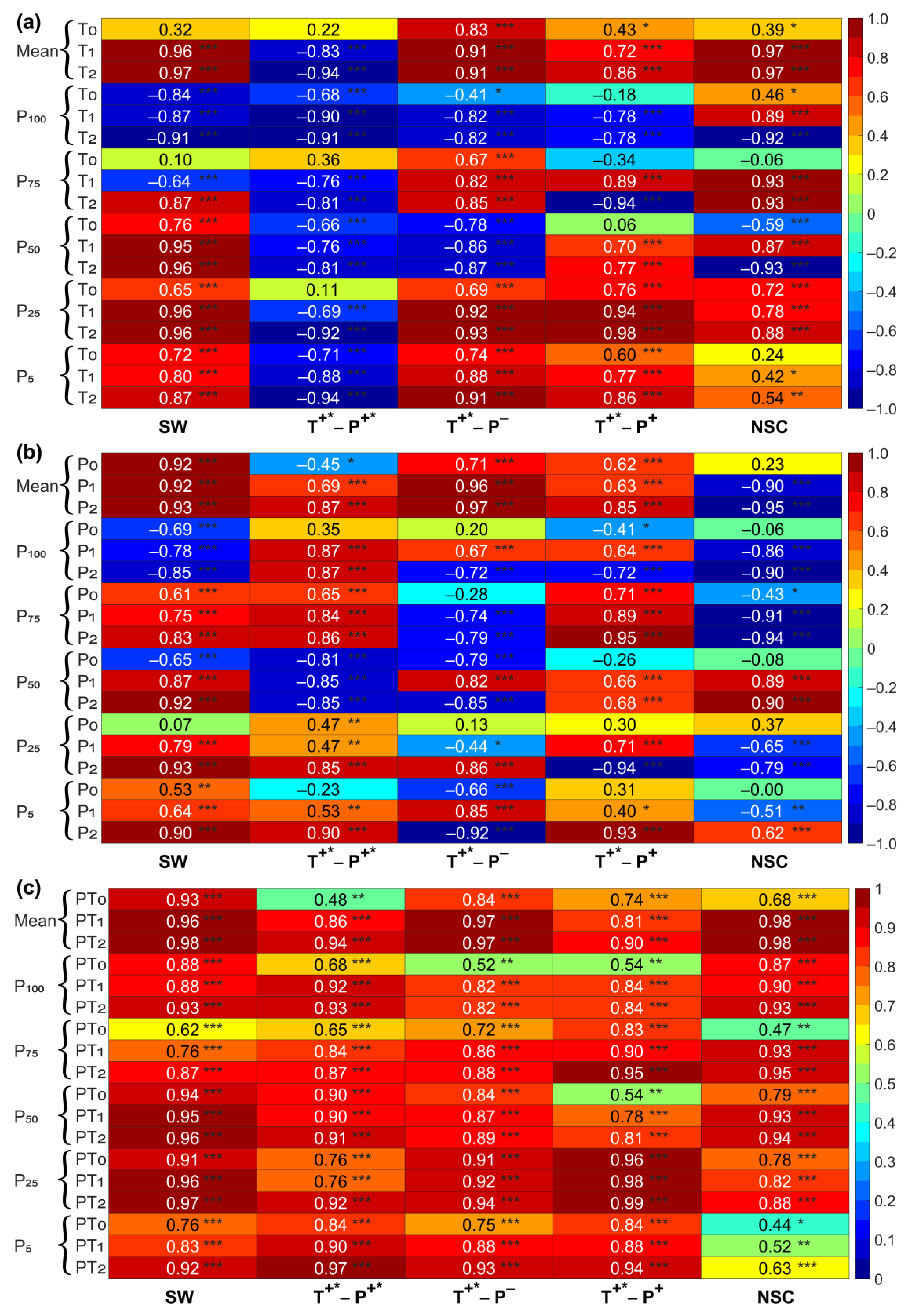
Under the condition of controlling the influence of precipitation (Figure 4a), the significantly negative delay responses of temperature on vegetation were mainly concentrated in T+*-P+*, P100, P75 in SW and T+*-P+, P50 in T+*-P−, and NSC, whereas elsewhere there were more significant positive delay responses. It can also be seen from Figure 4b that under the condition of controlling temperature, the significantly negative time delay response of vegetation to precipitation was mainly concentrated in T+*-P− and NSC (except Mean) as were the P100 period in the SW and the P50 period in the T+*-P+*. In other cases, the time delay response of vegetation was mainly significantly positive. When the time delay effect was taken into account, the mean value of the precipitation diphasic coefficient |R| at P100, P50–P5 was less than that of the temperature diphasic coefficient |R|. Taking the time delay effect into consideration, the correlation coefficient of the annual time delay of temperature and precipitation on vegetation increased by 0.15 (24.48%)–0.51 (165.77%) and 0.23 (39.93%)–0.42 (128.48%), respectively, and the interannual delay increased by 0.22 (36.53%)–0.57 (188.68%) and 0.32 (56.16%)–0.61 (227.23%), respectively, compared to the same period. The complex correlation coefficients (Figure 4c) achieved the significance level of p < 0.05 when the annual and interannual time delays were considered, and this was successively increased by 0.02–0.20 (2.73%–30.28%) and 0.08–0.24 (8.73%~37.19%), respectively, compared to the same period. The mean values were 0.87 and 0.91, respectively. The variance analysis showed that the |R| and |FR| of temperature and precipitation alone and in combination significantly improved (p < 0.05) when the time delay effect was considered. This suggested that when considering the time delay, the correlation between vegetation development and climate factors was greater and that there was a certain delay, which—when the lag correlation coefficient was taken into account—increased further; the average of the complex correlation coefficients |FR| was greater than 0.85 and reached as high as 0.87 and 0.91, suggesting that the reaction of vegetation to climate changes reflected the complexity of multidimensional space.
3.3. The Intensity Variation Trend of the Delayed Effect of Climate Factors on Vegetation
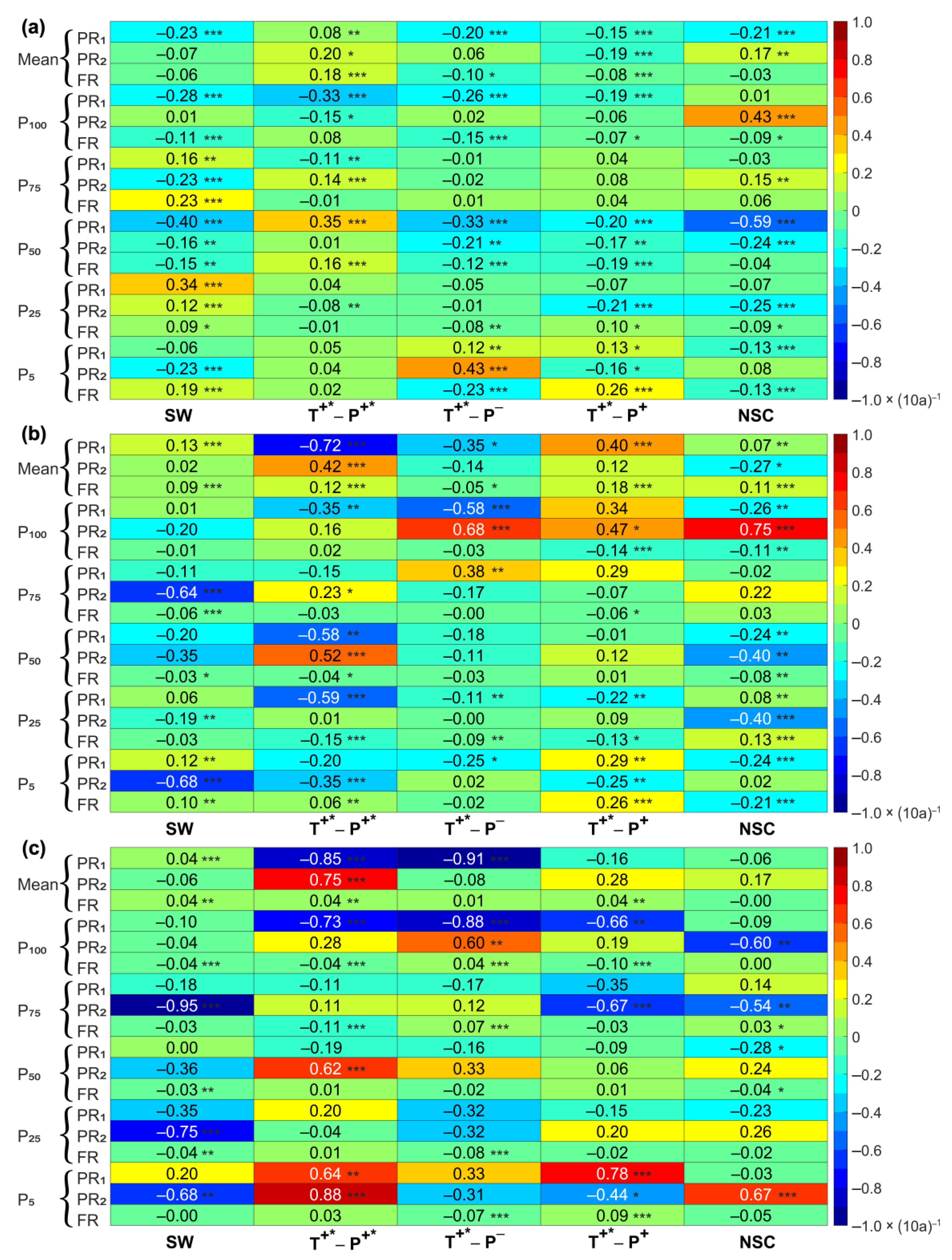
The temporal changes of vegetation reaction to climate changes at particular times (the same period, the particular year considered, and the interannual year considered) in the SW and the CA showed different directionality (Figure 5). With the time delay effect of NDVI (that is, when the time delay effect was not taken into account), the vegetation growth in different periods (six annual characteristic values) was affected by temperature, and the vegetation growth in SW, T+*-P−, T+*-P+, and NSC showed a decreasing trend. In contrast, the vegetation development in T+*-P+* appeared to show a significantly decreasing trend at P100 and P75. Furthermore, under the influence of precipitation, there was a decreasing trend in SW and T+*-P+ and at P100 and P25 in T+*-P+*, P75 to P25 in T+*-P−, and P50 to P25 in NSC. The impact of two climate factors showed a decreasing trend in T+*-P− and NSC, and at the Mean, P100, and P50 in SW, and T+*-P+ and the P75 and P25 in T+*-P+*. When the annual time delay effect was considered, the vegetation was affected by temperature, and the influence of temperature generally decreased in T+*-P+*, T+*-P−, and NSC and in the P75 to P50 in SW and P50 to P25 in T+*-P+. Under the influence of precipitation, in SW, T+*-P− and at Mean and P50~P25 in NSC, P75 and P5 periods in T+*-P+ showed a decreasing trend, whereas T+*-P+* showed a generally increasing trend. Under combined action, there was a predominantly decreasing trend.
When the interannual time delay effect was considered, vegetation was mainly affected by temperature, which showed a decreasing trend. Furthermore, precipitation affected vegetation, which showed a decreasing trend in SW and at Mean, P25, and P5 periods in T+*-P−, P75, and P5 periods in T+*-P+ and at P100 and P75 in NSC, whereas in the T+*-P+*, it exhibited an expanding drift. Under the impact of temperature and precipitation, the vegetation was affected by climate factors in SW, NSC, and at P100-P75 in T+*-P+*; P50-P5 in T+*-P− and P100-P75; and at P25 in T+*-P+, it exhibited a decreasing trend.
4. Discussion
4.1. Considering the Time Delay Effect Could Significantly Improve the Prediction Rate of the Effect of Climate on Vegetation Change
The correlation between climate factors and NDVI has been widely confirmed at landscape, regional, and global levels [11,13,14,16,21,22,23]. This study also confirmed that compared to the interpretation rate for the same period, considering the time delay effect (annual and interannual delay), the interpretation rates for temperature and precipitation factors and their combined effects on NDVI were significantly increased by 17.97% (43.78%) and 23.31% (56.79%), 20.15% (52.92%) and 27.21% (71.47%), and 18.48% (31.85%) and 25.32% (43.63%), respectively, and this was consistent with research results concerning the influence of most temperature and precipitation factors on vegetation delay [11,14,15,16]. Jia et al. [15] found that the impact of temperature and precipitation on vegetation in the Xijiang River Basin in southern China reached significant levels of 31.47% and 32.99%, respectively, when accounting for the time delay effect. Zhao et al. [16] found that the explanation rate of climate factors (temperature and precipitation) in the same period (without the time delay effect) was less than 10%, but when time delay was taken into account, the relative increase was over 95%. Wu et al. [11] showed that accounting for time delay effects could increase the rate of global vegetation growth explained by climate factors by 11%. In our study, when the time delay effect was considered, the improvement was more significant, particularly in the T+*-P+* in the P75 period, in which the temperature to NDVI increased by 39.80% (2080.92%). In the T+*-P+* in the P100 period, the explanation rate of NDVI by precipitation increased by 52.09% (5482.63%).
When considering the annual time delay effect, at Mean and P100–P5 periods, the averages of the optimal time delays were 1.60, 3.40, 2.20, 3.80, 0.40, and 1.00, respectively, and were in the main 0–4 months, results which were essentially consistent with the findings of Wu et al. [11] and Ding et al. [14] at the global level, Gessner et al. [49] for central Asia, Piao et al. [1] for northern Eurasia, Workie and Debella [22] for Ethiopia, and Daham et al. [13] for Sulaimaniyah and Wasit. This study also identified several optimal time lags longer than four months. For example, in the SW in the P100 period, the time lag of temperature on vegetation growth was seven months, and in the P50 period, the time lag of precipitation on vegetation growth was nine months. Similarly, Tei et al. [23] pointed out that the forest ecosystem in the Arctic Circle between 50°N–67°N was driven by the temperature and precipitation factors of the previous year (from summer to winter); Zhao et al. [12] suggested that vegetation in the Amazon region had a time lag of 0–6 months to temperature; and Braswell et al. [50] found that NDVI had a 2-year lag reaction to temperature. Our further analysis showed that although the optimal time delay considering the annual delay effect was concentrated in 0–4 months, the optimal time delay relating to temperature and precipitation was not entirely synchronized, and the time delay for temperature (3.40 and 0.40 months) was more extensive than that for precipitation (2.40 and 0.20 months) in the P100 and P25 period. These findings were similar to those of Ye et al. [28] in the high mountainous locale of southern Xizang, where vegetation was more sensitive to precipitation than temperature. Conversely, the time delay for precipitation (1.60 months) was more extensive than that for temperature (2.8 months) at Mean, which was similar to the findings of Workie and Debella [22] in Ethiopia and Gu et al. [27] in the Red River Basin in southern China. These researchers found that the reaction of NDVI to temperature was faster than it was to precipitation. However, at periods P75, P50, and P5, the two delays were equal.
When all the results were integrated, it was further found that the P25 period was the period with the maximum or submaximum explanation rate, whether within the same period or when time delay effects were taken into account, rather than the annual maximum or average combined results commonly used by most scholars (Figure 3). Combined with the results in Figure A1, it can be seen that the P100 and P75 in the vigorous plant growth period mainly occurred from June to August (summer) in the entire SW and CA, that vegetation development entered a relatively stable state and was less dependent on temperature and precipitation, and that there was sufficient hydrothermal energy to meet vegetation development needs [16]. Summer is the season in which precipitation is intensively dispersed within the considered zone; during summer, there is a large amount of water vapor in the air and the area is prone to rainfall and cloudy weather. Furthermore, the GIMMS NDVI data had been obtained using optical sensors, which are limited by the optical sensor characteristics [51] and were greatly affected by the suspension and scattering of external weather (cloud, fog, etc.) and aerosol in the atmospheric components [52]. Even though the data set had been pretreated using geometric, radiometric, and atmospheric correction, cloud interference could be further eliminated through filtering [44]. Since there are fewer valid images from June to August, the reliability of the images decreases.
4.2. Considering the Time Delay Effect Could Significantly Improve the Response Intensity of Vegetation to Climate
When the time delay effect was considered, the response intensity of vegetation to temperature, precipitation, and their interaction was significantly improved, which was consistent with the findings of most researchers [11,13,14,16,21,22,23]. However, the direction of the response strength was not uniform. In the P100 period, NDVI was mainly adversely connected to temperature, demonstrating that within the most vigorous vegetation growth period (P100), this occurred from July to August of a year (i.e., summer) (Figure A1), and the optimal time delay was 3.40 months when the annual delay effect was taken into account. This proved that the temperature 3.40 months before the most vigorous period of vegetation growth (from about 3.6 months to 4.6 months, i.e., from mid–late March to mid–late April) had already met the heat required for vegetation growth (Figure 2a). When the temperature increased and exceeded the optimum temperature, photosynthetic enzyme activity [53] and potential photosynthetic utilization capacity [20] would be enhanced, evaporation would be accelerated, and water utilization reduced, thus inhibiting plant development [10,11,54,55]. When the temperature of the month in which the optimal interannual delay occurs increased (the optimal time delay was 7.80 months, which was roughly during the 11.2–12.2 months of the previous year, i.e., early November to early December), this reduces the cold shock effect of the temperature on vegetation. When the temperature cold shock effect decreased, the accumulated temperature required for vegetation leaf-spreading increased [47], further aggravating evaporation, reducing soil moisture, and affecting vegetation growth the following year. Tei et al. [23] also obtained the same results, describing how the previous year’s temperature damaged the ecosystem in the woodlands around the Arctic Circle between 50°N and 67°N.The primarily negative relationship between NDVI and temperature appeared in T+*-P+*—the higher the temperature, the lower the NDVI. This might be because of the T+*-P+* in the northwest, which is part of the plateau that shapes the semi-arid zone (as shown in Table 1), where there was less rainfall and the soil moisture content was low, so that when temperature increased, soil temperature also increased, resulting in accelerated evaporation and reduced water availability [28,54], further aggravating soil water shortage and aridity [10] and also threatening plant growth and photosynthesis [10,11]. The intensity of the reaction of vegetation to precipitation was mostly negatively correlated at P100–P5 periods in T+*-P− and NSC, indicating that the more precipitation, the lower the NDVI, which may be because T+*-P– and NSC belong to the moist subtropical area, the humid subtropical humid temperate semi-humid zone, and the plateau area (as shown in Table 1). Here, high precipitation increased the soil moisture content and directly influenced the development of vegetation, and the more significant the precipitation, the more waterlogged the soil became, which lowered the temperature of the surrounding environment, reduced solar radiation [25,31], and offset the positive effect of precipitation on vegetation. In addition, soil became more susceptible to erosion because of higher precipitation, and according to the RULSE loss equation, increased soil loss would inhibit vegetation growth [56]. Under other conditions, the correlation was primarily positive in that increased precipitation replenished soil water, and plants absorbed the water through their roots and transported water to the leaves for photosynthesis, thus increasing chlorophyll and promoting vegetation growth [14,25,57]. Similarly, some researchers have detected a strong positive relationship between vegetation change and precipitation in the southwestern United States [29], the Australian outback [21], the Yun–Gui Plateau [30], and Sulaimaniyah [13]. When considering the annual and interannual delay effect, the complex correlation coefficients increased significantly (p < 0.05), reaching 0.87 and 0.91, respectively, which indicated that vegetation development was closely related to changes in precipitation and temperature. Climate change has significantly affected and played a critical part in the development of terrestrial vegetation [1,3,4,5,11,13,14,16,21,22,23].
4.3. The Phased Responses of Vegetation to Climate Change
Based on the results shown in Figure 2, Figure 3, and Figure 4 and the findings of previous studies, it has been demonstrated that climate change significantly affects the growth of terrestrial vegetation. We analyzed the correlation between NDVI and climatic factors (temperature and precipitation) over 15-year time periods, and the decreasing trend was dominant both for the same period and also when (annual and interannual) time delay effects were taken into account. This indicated that with continued global warming, the impact of climate factors on vegetation development tended to decrease, which may result from changes in other surrounding environmental factors connected with global warming, altering the relationship between climate and vegetation over time [58,59,60,61,62,63]. When the temperature increases and exceeds the optimum temperature for vegetation photosynthesis and evaporation accelerates, the probability of vegetation being subjected to drought stress is increased, and this changes the way in which plant development reacts to temperature change. The influence of drought also weakens the response of NDVI to temperature change [55,59], and higher temperatures lead to increased plant respiration, which in turn affects net primary production through consumption of organic matter [64]. As more water is needed for vegetation growth, an increase in precipitation can supplement soil water, the primary source of water in the soil, and plants can absorb water through their roots and promote vegetation growth [16]. However, when the precipitation surpassed a certain threshold, the correlation between NDVI and precipitation showed a diminishing trend [60,63]. D’Arrigo et al. [65] pointed out that the increase in temperature was the potential reason why tree development became less sensitive to temperature in the second half of the 20th century. Piao et al. [58] confirmed that the correlation between NDVI and temperature during the developing season would be weakened because of the continuous warming of the Northern Hemisphere. Fu et al. [47] also proved that global warming had reduced the cold shock temperature for vegetation and that the lower the cold shock temperature, the higher the required accumulated temperature for vegetation leaf expansion, which further reduced soil moisture, affected leaf expansion the following spring, and reduced the growth of vegetation.
5. Conclusions
This research attempted to establish the impact of climate factors on vegetation growth, which was difficult to quantify and had a lower explanation rate, and explored the reaction characteristics of vegetation to climate change. The changing trend of reaction intensity generated the following research questions: (1) How can the optimal time lag for the impact of climate factors on vegetation growth be determined? (2) How can the trend of the intensity of the time delay reaction of vegetation to climate change be characterized and quantified? To answer these questions, we used CRU and GIMMS NDVI data to explore the changing trend of the optimal delay response and the response intensity of vegetation to single and multiple factors in different periods (P100–P5 and Mean) in SW and CAs. Generally, we found that in the different growth periods of vegetation (P100–P5 and Mean) across the entire SW and CA, the prediction rate of climate change on vegetation development was significantly improved when the (annual and interannual) time lag impact was taken into account, and we also proved that the reaction of vegetation change to meteorological factors had a specific time lag. The response was more significant when the interannual time lag effect was taken into consideration. Vegetation growth has gradually reduced under the influence of climate change, which may be the result of other surrounding environmental factors which are also affected by global warming, causing the relationship between climate and vegetation to alter over time. The optimal synthesis of the NDVI annual value may be in the P25 period rather than the annual maximum value or annual mean value commonly used by most scholars. To an extent, our study provides a relevant theoretical basis for analyzing, predicting, and evaluating the dynamic response of vegetation and its reaction to climatic alterations against the background of global climate change.
Author Contributions
Conceptualization, M.W.; methodology, M.W. and S.W.; software, M.W. and S.W.; validation, M.W. and Z.A.; formal analysis, M.W. and S.W; investigation, M.W.; resources, M.W.; data curation, M.W.; writing—original draft preparation, M.W. and Z.A.; writing—review and editing, M.W. and Z.A.; visualization, M.W.; supervision, M.W.; project administration, M.W.; funding acquisition, M.W. All authors have read and agreed to the published version of the manuscript.
Funding
This research was funded by the Chaozhou Special Fund for Human Resource Development, grant number 2022.
Data Availability Statement
The NDVI datasets used in our work can be freely accessed at https://ecocast.arc.nasa.gov/data/pub/GIMMS/, accessed on 18 November 2018. The climate data (CRU_TS4.02) were obtained from https://crudata.uea.ac.uk/cru/data/hrg/, accessed on 18 December 2018.
Conflicts of Interest
The authors declare no conflict of interest.
Appendix A
Screening Steps for the Occurrence Month of the Six Annual Characteristic Values
- (1)
- Preprocessing: using 15 years as a sliding window, the NDVI series of 1982–1996, 1983–1997, …, 2001–2015 were successively screened, resulting in 20 windows, after which a new NDVI matrix sequence was generated (Figure A1).
- (2)
- Calculating eigenvalue: according to the method described by Wang and An [32], the annual maximum (P100), upper quarter quantile (P75), median (P50), lower quarter quantile (P25), minimum (P5), and mean (Mean) of GIMMSNDVI in each time period were screened out, and then the NDVI eigenvalue sequence was regenerated.
- (3)
- Calculation relative frequency: the frequencies for each month were counted and then divided by the total number of 20 windows to obtain the relative frequency for each month.
- (4)
- The screening principles for the occurrence month: (1) the month with the most significant relative frequency was the month with the occurrence of an eigenvalue; and (2) if the frequency was the same, the month with the smaller number was defined as the occurrence month.
Appendix B
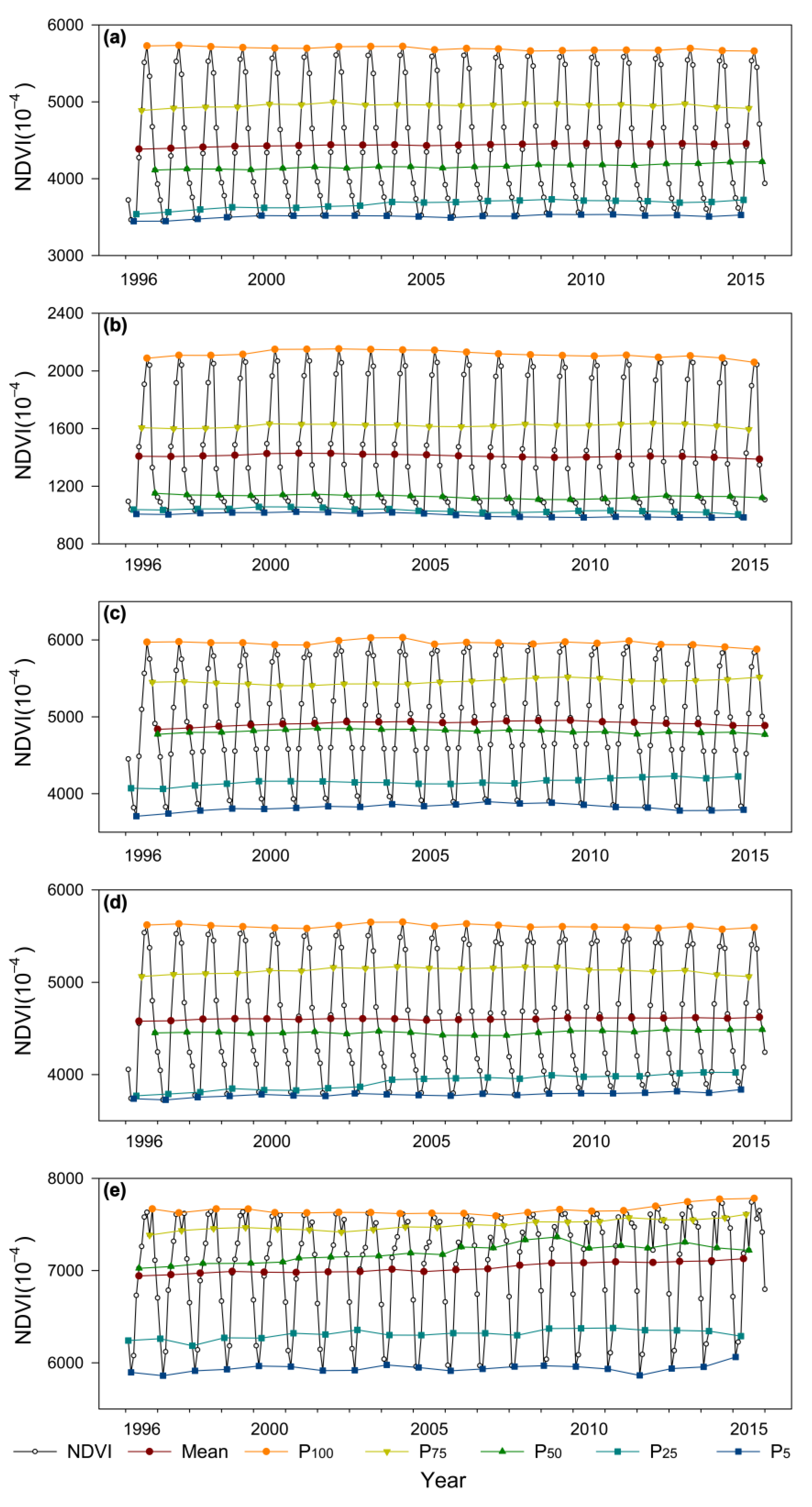
Figure A1.
Changes in NDVI during each year of the 15-year windows. The horizontal axis is the upper limit year of the 15-year moving window, with 1996, 1997, …, 2015, representing the mobile windows of 1982–1996, 1983–1997, …, and 2001–2015, respectively. P100, P75, P50, P25, and P5, individually represent the filter month in which the occurrence occurs from the moving window, and the Mean refers to the month closest to the Mean. (a–e) separately refer to the SW, T+*-P+*, T+*-P−, T+*-P+, and NSC.

References
- Piao, S.L.; Wang, X.; Ciais, P.; Zhu, B.; Wang, T.; Liu, J.I.E. Changes in satellite-derived vegetation growth trend in temperate and boreal Eurasia from 1982 to 2006. Glob. Chang. Biol. 2011, 17, 3228–3239. [Google Scholar] [CrossRef]
- Shen, X.J.; Liu, B.H.; Zhou, D.W. Using GIMMS NDVI time series to estimate the impacts of grassland vegetation cover on surface air temperatures in the temperate grassland region of China. Remote Sens. Lett. 2016, 7, 229–238. [Google Scholar] [CrossRef]
- IPCC. Special Report on Global Warming of 1.5 °C; Cambridge University Press: Cambridge, UK, 2018. [Google Scholar]
- IPCC. Climate Change 2021, The physical science basis. In Contribution of Working Group, I to the Sixth Assessment Report of the Intergovernmental Panel on Climate Change; Cambridge University Press: Cambridge, UK, 2021. [Google Scholar]
- Gao, J.; Jiao, K.; Wu, S. Investigating the spatially heterogeneous relationships between climate factors and NDVI in China during 1982 to 2013. J. Geogr. Sci. 2019, 29, 1597–1609. [Google Scholar] [CrossRef] [Green Version]
- Nemani, R.R.; Keeling, C.D.; Hashimoto, H.; Jolly, W.M.; Piper, S.C.; Tucker, C.J.; Myneni, R.B.; Running, S.W. Climate-driven increases in global terrestrial net primary production from 1982 to 1999. Science 2003, 300, 1560–1563. [Google Scholar] [CrossRef] [Green Version]
- Cui, L.; Shi, J.; Xiao, F.; Fan, W. Variation trends in vegetation NDVI and its correlation with climatic factors in Eastern China. Res. Sci. 2010, 32, 124–131. [Google Scholar]
- Chen, Y.; Luo, Y.; Mo, W.; Mo, J.; Huang, Y.; Ding, M. Differences between MODIS NDVI and MODIS EVI in response to climatic factors. J. Nat. Res. 2014, 29, 1802–1812. [Google Scholar]
- He, B.; Chen, A.; Wang, H.; Wang, Q. Dynamic response of satellite-derived vegetation growth to climate change in the Three North Shelter Forest Region in China. Remote Sens. 2015, 7, 9998–10016. [Google Scholar] [CrossRef] [Green Version]
- Huang, X.; Zhang, T.B.; Yi, G.H.; He, D.; Zhou, X.B.; Li, J.J.; Bie, X.J.; Miao, J.Q. Dynamic changes of NDVI in the growing season of the Tibetan Plateau during the past 17 years and its response to climate change. Int. J. Environ. Res. Public Health 2019, 16, 3452. [Google Scholar] [CrossRef] [Green Version]
- Wu, D.; Zhao, X.; Liang, S.; Zhou, T.; Huang, K.; Tang, B.; Zhao, W. Time-lag effects of global vegetation responses to climate change. Glob. Chang. Biol. 2015, 21, 3520–3531. [Google Scholar] [CrossRef]
- Zhao, W.; Zhao, X.; Zhou, T.; Wu, D.; Tang, B.; Wei, H. Climatic factors driving vegetation declines in the 2005 and 2010 Amazon droughts. PLoS ONE 2017, 12, e0175379. [Google Scholar]
- Daham, A.; Han, D.; Rico-Ramirez, M.; Marsh, A. Analysis of NVDI variability in response to precipitation and air temperature in different regions of Iraq, using MODIS vegetation indices. Environ. Earth Sci. 2018, 77, 389. [Google Scholar] [CrossRef] [Green Version]
- Ding, Y.; Li, Z.; Peng, S. Global analysis of time-lag and -accumulation effects of climate on vegetation growth. Int. J. Appl. Earth Obs. 2020, 92, 102179. [Google Scholar] [CrossRef]
- Jia, L.; Li, Z.; Xu, G.; Ren, Z.; Li, P.; Cheng, Y.; Zhang, Y.; Wang, B.; Zhang, J.; Yu, S. Dynamic change of vegetation and its response to climate and topographic factors in the Xijiang River basin, China. Environ. Sci. Pollut. R. 2020, 27, 11637–11648. [Google Scholar] [CrossRef]
- Zhao, W.J. Extreme weather and climate events in China under changing climate. Natl. Sci. Rev. 2020, 7, 938–943. [Google Scholar] [CrossRef] [Green Version]
- Wang, D.; Alimohammadi, N. Responses of annual runoff, evaporation, and storage change to climate variability at the watershed scale. Water Resour. Res. 2012, 48, 5546. [Google Scholar] [CrossRef] [Green Version]
- Fu, Y.H.; Piao, S.L.; Delpierre, N.; Hao, F.; Hänninen, H.; Liu, Y.; Sun, W.; Janssens, I.A.; Campioli, M. Larger temperature response of autumn leaf senescence than spring leaf–out phenology. Glob. Chang. Biol. 2017, 24, 2159–2168. [Google Scholar] [CrossRef]
- Kong, D.; Miao, C.; Borthwick, A.G.L.; Lei, X.; Li, H. Spatiotemporal variations in vegetation cover on the Loess Plateau, China, between 1982 and 2013, possible causes and potential impacts. Environ. Sci. Pollut. R. 2018, 25, 13633–13644. [Google Scholar] [CrossRef] [Green Version]
- Liu, Q.; Fu, Y.H.; Zhu, Z.; Liu, Y.; Liu, Z.; Huang, M.; Janssens, I.A.; Piao, S. Delayed autumn phenology in the Northern Hemisphere is related to change in both climate and spring phenology. Glob. Chang. Biol. 2016, 22, 3702–3711. [Google Scholar] [CrossRef]
- Seddon, A.W.R.; Macias-Fauria, M.; Long, P.R.; Benz, D.; Willis, K.J. Sensitivity of global terrestrial ecosystems to climate variability. Nature 2016, 531, 229. [Google Scholar] [CrossRef] [Green Version]
- Workie, T.G.; Debella, H.J. Climate change and its effects on vegetation phenology across ecoregions of Ethiopia. Glob. Ecol. Conserv. 2017, 13, e00366. [Google Scholar] [CrossRef]
- Tei, S.; Sugimoto, A. Time lag and negative responses of forest greenness and tree growth to warming over circumboreal forests. Glob. Chang. Biol. 2018, 24, 4225–4237. [Google Scholar] [CrossRef] [PubMed]
- Peng, J.; Wu, C.Y.; Zhang, X.Y.; Wang, X.Y.; Gonsamo, A. Satellite detection of cumulative and lagged effects of drought on autumn leaf senescence over the Northern Hemisphere. Glob. Chang. Biol. 2019, 25, 2174–2188. [Google Scholar] [CrossRef] [PubMed]
- Piao, S.L.; Mohammat, A.; Fang, J.; Cai, Q.; Feng, J. NDVI-based increase in growth of temperate grasslands and its responses to climate changes in China. Glob. Environ. Chang. 2006, 16, 340–348. [Google Scholar] [CrossRef]
- Chen, X.; An, S.; Inouye, D.; Schwartz, M.D. Temperature and snowfall trigger alpine vegetation green-up on the world’s roof. Glob. Chang. Biol. 2015, 21, 3635–3646. [Google Scholar] [CrossRef] [PubMed]
- Gu, Z.; Duan, X.; Shi, Y.; Li, Y.; Pan, X. Spatiotemporal variation in vegetation coverage and its response to climatic factors in the Red River Basin, China. Ecol. Indic. 2018, 93, 54–64. [Google Scholar] [CrossRef]
- Ye, Z.; Cheng, W.; Zhao, Z.; Guo, J.; Ding, H.; Nan, W. Interannual and Seasonal Vegetation Changes and Influencing Factors in the Extra-High Mountainous Areas of Southern Tibet. Remote Sens. 2019, 11, 1392. [Google Scholar] [CrossRef] [Green Version]
- Zhang, X.; Goldberg, M.; Tarpley, D.; Friedl, M.A.; Morisette, J.; Kogan, F.; Yu, Y. Drought induced vegetation stress in southwestern North America. Environ. Res. Lett. 2010, 5, 024008. [Google Scholar] [CrossRef]
- Qiu, B.W.; Li, W.J.; Zhong, M.; Tang, Z.H.; Chen, C.C. Spatiotemporal analysis of vegetation variability and its relationship with climate change in China. Geo-Spat. Inf. Sci. 2014, 17, 170–180. [Google Scholar] [CrossRef] [Green Version]
- Guo, L.; Zuo, L.; Gao, J.; Jiang, Y.; Zhang, Y.; Ma, S.; Zou, Y.; Wu, S. Revealing the Fingerprint of Climate Change in Interannual NDVI Variability among Biomes in Inner Mongolia, China. Remote Sens. 2020, 12, 1332. [Google Scholar] [CrossRef] [Green Version]
- Wang, M.; An, Z. Regional and Phased Vegetation Responses to Climate Change Are Different in Southwest China. Land 2022, 11, 1179. [Google Scholar] [CrossRef]
- Li, X.C. Historical Geography, Geopolitics, Regional Economy and Culture; Peking University Press: Beijing, China, 2004; pp. 79–93. (In Chinese) [Google Scholar]
- Wang, M.; Jiang, C.; Sun, O.J. Spatially differentiated changes in regional climate and underlying drivers in southwestern China. J. For. Res. 2022, 33, 755–765. [Google Scholar] [CrossRef]
- You, Q.; Chen, D.; Wu, F.; Pepin, N.; Cai, Z.; Ahrens, B.; Jiang, Z.; Wu, Z.; Kang, S.; Amir, A.K. Elevation dependent warming over the Tibetan Plateau, Patterns, mechanisms and perspectives. Earth-Sci. Rev. 2020, 210, 103349. [Google Scholar] [CrossRef]
- Harris, I.; Osborn, T.; Jones, P.; Lister, D. Version 4 of the CRU TS monthly high-resolution gridded multivariate climate dataset. Sci. Data 2020, 7, 1–18. [Google Scholar] [CrossRef] [PubMed]
- Buermann, W.G.; Forkel, M.; O’Sullivan, M.; Sitch, S.; Friedlingstein, P.; Haverd, V. Widespread seasonal compensation effects of spring warming on northern plant productivity. Nature 2018, 562, 110–115. [Google Scholar] [CrossRef] [Green Version]
- China Meteorological Administration. Blue Book on Climate Change in China 2020; Science Press: Beijing, China, 2020. [Google Scholar]
- Wang, H.; Liu, H.; Cao, G.; Sanders, N.J.; Classen, A.T.; He, J.S. Alpine grassland plants grow earlier and faster but biomass remains unchanged over 35 years of climate change. Ecol. Lett. 2020, 23, 701–710. [Google Scholar] [CrossRef] [Green Version]
- Grosso, S.D.; Parton, W.J.; Derner, J.; Chen, M.; Compton, J.T. Simple models to predict grassland ecosystem C exchange and actual evapotranspiration using NDVI and environmental variables. Agric. For. Meteorol. 2018, 249, 1–10. [Google Scholar] [CrossRef]
- Pepin, N.; Bradley, R.S.; Diaz, H.F.; Baraer, M.; Caceres, E.B.; Forsythe, N.; Fowler, H.; Greenwood, G.; Hashmi, M.Z.; Liu, X.D.; et al. Elevation-dependent warming in mountain regions of the world. Nat. Clim. Chang. 2015, 5, 424–430. [Google Scholar]
- Li, X.P.; Wang, L.; Guo, X.Y.; Chen, D.L. Does summer precipitation trend over and around the Tibetan Plateau depend on elevation? Int. J. Climatol. 2017, 37, 1278–1284. [Google Scholar] [CrossRef]
- Knott, G.D. Interpolating Cubic Splines; Springer Science & Business Media: Berlin, Germany, 2012; pp. 1–244. [Google Scholar]
- Yin, L.; Wang, X.; Feng, X.; Fu, B.; Chen, Y. A Comparison of SSEBop-Model-Based Evapotranspiration with Eight Evapotranspiration Products in the Yellow River Basin, China. Remote Sens. 2020, 12, 2528. [Google Scholar] [CrossRef]
- Gong, P.; Li, X.; Wang, J.; Bai, Y.; Zhou, Y. Annual maps of global artificial impervious area (GAIA) between 1985 and 2018. Remote Sens. Environ. 2020, 236, 111510. [Google Scholar] [CrossRef]
- Yuan, J.J.; Guo, J.Y.; Niu, Y.P.; Zhu, C.C.; Li, Z. Mean Sea Surface Model over the Sea of Japan Determined from Multi-Satellite Altimeter Data and Tide Gauge Records. Remote Sens. 2020, 12, 4168. [Google Scholar] [CrossRef]
- Fu, Y.; Zhao, H.; Piao, S.L.; Peaucelle, M.; Peng, S.; Zhou, G.; Ciais, P.; Huang, M.T.; Menzel, A.; Penuelas, J.; et al. Declining global warming effects on the phenology of spring leaf unfolding. Nature 2015, 526, 104–107. [Google Scholar] [CrossRef] [PubMed] [Green Version]
- Arnone, J.A.; Verburg, P.S.; Johnson, D.W.; Wallace, L.L.; Luo, Y.Q.; Schimel, D.S. Prolonged suppression of ecosystem carbon dioxide uptake after an anomalously warm year. Nature 2008, 455, 383. [Google Scholar] [CrossRef] [PubMed]
- Gessner, U.; Naeimi, V.; Klein, I.; Kuenzer, C.; Klein, D.; Dech, S. The relationship between precipitation anomalies and satellite-derived vegetation activity in Central Asia. Glob. Planet. Chang. 2012, 110, 74–87. [Google Scholar] [CrossRef]
- Braswell, B.H.; Schimel, D.S.; Linder, E.; Moore, B., III. The response of global terrestrial ecosystems to interannual temperature variability. Science 1997, 278, 870–873. [Google Scholar] [CrossRef]
- Li, P.; Peng, C.; Wang, M.; Luo, Y.; Li, M.; Zhang, K.; Zhang, D.; Zhu, Q. Dynamics of vegetation autumn phenology and its response to multiple environmental factors from 1982 to 2012 on Qinghai-Tibetan Plateau in China. Sci. Total. Environ. 2018, 637–638, 855–864. [Google Scholar] [CrossRef]
- Nagol, J.R.; Vermote, E.F.; Prince, S.D. Effects of atmospheric variation on AVHRR NDVI data. Remote Sens. Environ. 2009, 113, 392–397. [Google Scholar] [CrossRef]
- Shi, C.; Sun, G.; Zhang, H.; Xiao, B.; Ze, B.; Zhang, N.; Wu, N. Effects of warming on chlorophyll degradation and carbohydrate accumulation of alpine herbaceous apecies during plant senescence on the Tibetan Plateau. PLoS ONE 2014, 9, e107874. [Google Scholar] [CrossRef] [Green Version]
- Vicente-Serrano, S.M.; Gouveia, C.; Camarero, J.J.; Revuelto, J.; Morán-Tejeda, E.; Sanchez-Lorenzo, A. Response of vegetation to drought time-scales across global land biomes. Proc. Natl. Acad. Sci. USA 2013, 110, 52–57. [Google Scholar] [CrossRef] [Green Version]
- Yan, H.; Yu, Q.; Zhu, Z.C.; Myneni, R.B.; Yan, H.M.; Wang, S.Q.; Shugart, H.H. Diagnostic analysis of interannual variation of global land evapotranspiration over 1982–2011, assessing the impact of ENSO. J. Geophys. Res. Atmos. 2013, 118, 8969–8983. [Google Scholar] [CrossRef]
- Xiong, M.Q.; Sun, R.H.; Chen, L.D. A global comparison of soil erosion associated with land use and climate type. Geoderma 2019, 343, 31–39. [Google Scholar] [CrossRef]
- Chen, J.H.; Yan, F.; Luk, Q. Spatiotemporal Variation of Vegetation on the Qinghai-Tibet Plateau and the Influence of Climatic Factors and Human Activities on Vegetation Trend (2000–2019). Remote Sens. 2020, 12, 3150. [Google Scholar] [CrossRef]
- Piao, S.L.; Nan, H.; Huntingford, C.; Zeng, N.; Zeng, Z.; Chen, A. Evidence for a weakening relationship between interannual temperature variability and northern vegetation activity. Nat. Commun. 2014, 5, 5018. [Google Scholar] [CrossRef] [PubMed] [Green Version]
- Angert, A.; Biraud, S.; Bonfils, C.; Henning, C.C.; Buermann, W.; Pinzon, J.; Tucker, C.J.; Fung, I. Drier summers cancel out the CO2 uptake enhancement induced by warmer springs. Proc. Natl. Acad. Sci. USA 2005, 102, 10823–10827. [Google Scholar] [CrossRef]
- Chen, Q.; Zhou, Q.; Zhang, H.; Liu, F. Spatial disparity of NDVI response in vegetation growing season to climate change in the Three-River Headwaters Region. Ecol. Environ. Sci. 2010, 19, 1284–1289. [Google Scholar]
- Beck, P.S.; Goetz, S.J. Satellite observations of high northern latitude vegetation productivity changes between 1982 and 2008, ecological variability and regional differences. Environ. Res. Lett. 2011, 6, 045501. [Google Scholar] [CrossRef]
- IPCC. Climate Change 2013, The Physical Science Basis, Summary for Policymakers; Cambridge University Press: Cambridge, UK, 2013. [Google Scholar]
- Wu, Y.; Tang, G.; Gu, H.; Liu, Y.; Yang, M.; Sun, L. The variation of vegetation greenness and underlying mechanisms in Guangdong province of China during 2001–2013 based on MODIS data. Sci. Total. Environ. 2019, 653, 536–546. [Google Scholar] [CrossRef]
- Lu, H.P.; Dong, G.; Zhao, F.Y.; Qin, H. Impacts of Climatic Factors on Vegetation in the Loess Plateau. J. Shanxi U. Nat. Sci. Ed. 2018, 41, 626–635. (In Chinese) [Google Scholar]
- D’arrigo, R.D.; Kaufmann, R.K.; Davi, N.; Jacoby, G.C.; Laskowski, C.; Myneni, R.B.; Cherubini, P. Thresholds for warming-induced growth decline at elevational tree line in the Yukon Territory, Canada. Glob. Biogeochem. Cycles 2004, 18, GB3021. [Google Scholar] [CrossRef]
Figure 1.
Outline of (a) geography, (b) vegetation divisions, and (c) types of vegetation in the SW area.
Figure 1.
Outline of (a) geography, (b) vegetation divisions, and (c) types of vegetation in the SW area.

Figure 2.
Time delay effects on vegetation of (a) temperature factors and (b) precipitation factors over the 15-year periods. The numbers 1–24 represent the corresponding months, in which 1–12 represent January to December of the previous year; 13–24 represent January to December of the current year; and T1, T2, …, T24 and P1, P2, …, P24 represent the corresponding months of temperature and precipitation factors, respectively. ![Remotesensing 14 05580 i001]() No Data represents the occurrence months that exceed the NDVI eigenvalue,
No Data represents the occurrence months that exceed the NDVI eigenvalue, ![Remotesensing 14 05580 i002]() annual represents the maximum R2 when considering the annual time delay, and
annual represents the maximum R2 when considering the annual time delay, and ![Remotesensing 14 05580 i003]() interannual represents the maximum R2 when considering the interannual time delay. “*”, “**”, and “***” demonstrate the importance of p < 0.1, p < 0.05, and p < 0.01, respectively.
interannual represents the maximum R2 when considering the interannual time delay. “*”, “**”, and “***” demonstrate the importance of p < 0.1, p < 0.05, and p < 0.01, respectively.
 No Data represents the occurrence months that exceed the NDVI eigenvalue,
  annual represents the maximum R2 when considering the annual time delay, and
  interannual represents the maximum R2 when considering the interannual time delay. “*”, “**”, and “***” demonstrate the importance of p < 0.1, p < 0.05, and p < 0.01, respectively.
Figure 2.
Time delay effects on vegetation of (a) temperature factors and (b) precipitation factors over the 15-year periods. The numbers 1–24 represent the corresponding months, in which 1–12 represent January to December of the previous year; 13–24 represent January to December of the current year; and T1, T2, …, T24 and P1, P2, …, P24 represent the corresponding months of temperature and precipitation factors, respectively. ![Remotesensing 14 05580 i001]() No Data represents the occurrence months that exceed the NDVI eigenvalue,
No Data represents the occurrence months that exceed the NDVI eigenvalue, ![Remotesensing 14 05580 i002]() annual represents the maximum R2 when considering the annual time delay, and
annual represents the maximum R2 when considering the annual time delay, and ![Remotesensing 14 05580 i003]() interannual represents the maximum R2 when considering the interannual time delay. “*”, “**”, and “***” demonstrate the importance of p < 0.1, p < 0.05, and p < 0.01, respectively.
interannual represents the maximum R2 when considering the interannual time delay. “*”, “**”, and “***” demonstrate the importance of p < 0.1, p < 0.05, and p < 0.01, respectively.
No Data represents the occurrence months that exceed the NDVI eigenvalue, annual represents the maximum R2 when considering the annual time delay, and interannual represents the maximum R2 when considering the interannual time delay. “*”, “**”, and “***” demonstrate the importance of p < 0.1, p < 0.05, and p < 0.01, respectively.
Figure 3.
Time delay effects of multiple combinations of climate factors over the 15-year periods on vegetation. The numbers 1–24 represent the corresponding months, in which 1–12 represent January to December of the previous year, and 13–24 represent January to December of the current year, where T1, T2, …, T24 and P1, P2, …, P24 represent the corresponding months of temperature and precipitation factors, respectively. (a–f) refer to Mean, P100, P75, P50, P25, and P5, respectively. The numbers 1~5 of the lower indices refer to SW, T+*-P+*, T+*-P−, T+*-P+, and NSC, respectively. ![Remotesensing 14 05580 i001]() No Data represents the occurrence months that exceed the NDVI eigenvalue,
No Data represents the occurrence months that exceed the NDVI eigenvalue, ![Remotesensing 14 05580 i002]() annual represents the maximum R2 when considering the annual time delay, and
annual represents the maximum R2 when considering the annual time delay, and ![Remotesensing 14 05580 i003]() interannual represents the maximum R2 when considering the interannual time delay. “*”, “**”, and “***” demonstrate the importance of p < 0.1, p < 0.05, and p < 0.01, respectively.
interannual represents the maximum R2 when considering the interannual time delay. “*”, “**”, and “***” demonstrate the importance of p < 0.1, p < 0.05, and p < 0.01, respectively.
No Data represents the occurrence months that exceed the NDVI eigenvalue, annual represents the maximum R2 when considering the annual time delay, and interannual represents the maximum R2 when considering the interannual time delay. “*”, “**”, and “***” demonstrate the importance of p < 0.1, p < 0.05, and p < 0.01, respectively.

Figure 4.
The strength of the time lag effect of (a) the temperature factor, (b) the precipitation factor, and (c) multiple combinations of climate factors. T, P, and PT represent temperature, precipitation, and precipitation and temperature, respectively. The numbers 0, 1, and 2 of the lower indices represent the same period, respectively, considering the annual and interannual time lag. “*”, “**”, and “***” demonstrate the importance of p < 0.1, p < 0.05, and p < 0.01, respectively.

Figure 5.
The variation tendency of the correlation coefficient between NDVI and temperature and precipitation in a 15-year period considering (a) the same period, (b) the annual, and (c) the interannual time lag. PR1 and PR2 represent the partial correlation coefficient between NDVI and temperature and precipitation, respectively, and FR represents the multiple correlation coefficient. “*”, “**”, and “***” demonstrate the importance of p < 0.1, p < 0.05, and p < 0.01, respectively.


Table 1.
The source of primary data and related descriptions.
| Name | Sources | Resolution | Web Site | Access Date | Format |
|---|---|---|---|---|---|
| GIMMS NDVI3g | GIMMS | 8 × 8 km | https://ecocast.arc.nasa.gov/data/pub/GIMMS/ | 18 November 2018 | .nc4 |
| CRU_TS4.02 | Climate Research Unit | 0.5° × 0.5° | https://crudata.uea.ac.uk/cru/data/hrg/ | 28 June 2019 | .nc |
| Global Artificial Impervious Area | Tsinghua University data | 30 × 30 m | http://data.ess.tsinghua.edu.cn | 31 December 2019 | .tif |
| Digital elevation model | Resource and Environment Science and Data Center | 1 × 1 km | https://www.resdc.cn/data.aspx?DATAID=123 | 28 September 2019 | GRID |
| 1:1 million vegetation map of China | Resource and Environment Science and Data Center | — | https://www.resdc.cn/data.aspx?DATAID=122 | 1 December 2017 | .shp |
| China’s vegetation zoning data | Resource and Environment Science and Data Center | — | http://www.resdc.cn/data.aspx?DATAID=133 | 1 December 2017 | .shp |
Publisher’s Note: MDPI stays neutral with regard to jurisdictional claims in published maps and institutional affiliations. |
© 2022 by the authors. Licensee MDPI, Basel, Switzerland. This article is an open access article distributed under the terms and conditions of the Creative Commons Attribution (CC BY) license (https://creativecommons.org/licenses/by/4.0/).
Share and Cite
MDPI and ACS Style
Wang, M.; An, Z.; Wang, S. The Time Lag Effect Improves Prediction of the Effects of Climate Change on Vegetation Growth in Southwest China. Remote Sens. 2022, 14, 5580. https://doi.org/10.3390/rs14215580
AMA Style
Wang M, An Z, Wang S. The Time Lag Effect Improves Prediction of the Effects of Climate Change on Vegetation Growth in Southwest China. Remote Sensing. 2022; 14(21):5580. https://doi.org/10.3390/rs14215580
Chicago/Turabian StyleWang, Meng, Zhengfeng An, and Shouyan Wang. 2022. "The Time Lag Effect Improves Prediction of the Effects of Climate Change on Vegetation Growth in Southwest China" Remote Sensing 14, no. 21: 5580. https://doi.org/10.3390/rs14215580
Note that from the first issue of 2016, this journal uses article numbers instead of page numbers. See further details here.