Article

Impact of Smoke Plumes Transport on Air Quality in Sydney during Extensive Bushfires (2019) in New South Wales, Australia Using Remote Sensing and Ground Data

1
Atmospheric Science Department, Science Faculty, Mustansiriyah University, Baghdad 10011, Iraq
2
School of Earth, Atmospheric and Life Sciences, University of Wollongong, Wollongong, NSW 2522, Australia
*
Author to whom correspondence should be addressed.
Remote Sens. 2022, 14(21), 5552; https://doi.org/10.3390/rs14215552
Submission received: 2 September 2022 / Revised: 9 October 2022 / Accepted: 18 October 2022 / Published: 3 November 2022

Abstract

:
Smoke aerosol dispersion and transport have a significant impact on air quality levels and can be examined by environmental monitoring and modelling techniques. The purpose of this study is to determine the characteristics of the smoke aerosols and the level of air quality during November and December 2019 under the influence of extensive bushfires in the Sydney area, New South Wales (NSW), Australia. To achieve this goal, air quality and meteorological data were analysed in combination with remote sensing satellite measurements. Meteorological and air quality data were obtained from the Bureau of Meteorology (BOM) and Environmental Protection Agency monitoring sites in NSW. In Richmond the daily maximum average hourly concentration of particulate matter (PM10) was 848.9 μg/m3 at 07:00 UTC on 26 November 2019 and 785 μg/m3 at 07:00 UTC on 12 December 2019. On 10 December 2019, the highest PM10 recorded in the Sydney region was 961.5 μg/m3 in St Marys at 01:00 UTC, while the highest PM2.5 concentration was 714.6 μg/m3 in Oakdale in southwest Sydney at 18:00 UTC. These values all decreased again to the standard level (<50 μg/m3) in a few days. The potential sources of smoke aerosols originated from bushfires to the northwest of Sydney (Blue Mountains) as well as from southwest and northwest NSW. The smoke plumes were revealed by the combined AOD values from Aqua and Terra sensors on the MODIS satellite. In each case, the smoke travelled towards the east coast of Australia and out over the Pacific Ocean. The NAAPS model displays the existence of smoke at ground level, while the CALIPSO satellite data showed that the plumes extended 14 km up into the stratosphere layer. Backward trajectories obtained from the HYSPLIT model agree well with the movement of smoke plumes observed in the MODIS satellite images.

1. Introduction

Primary organic carbon and elemental carbon from bushfires represent the major aerosols originating from biomass burning [1,2,3,4]. Australia is one of the most exposed countries in the world to bushfires [5]. Elements that identify the extent of biomass burning include the burning period of the bushfires (blazing or smoking), the fuel kind, the temperature and the availability of oxygen [6]. Through the blazing stage, the emitted particle concentrations are larger, and the particles are smaller [7,8], compared with the smoke stage. In addition to CO2, gases such as CO, SO2 and NO2 are also emitted into the atmosphere during the blazing stage when bush fuel is completely burned [9]. Smaller quantities of other aerosols, such as sulphur, ammonia and nitrate, have also been detected during the blazing stage [10] and in the biomass burning stage [8,11].
In November–December 2019, a group of huge bushfires led to an increase in small particle pollution and ozone concentrations over the Sydney region. These bushfires covered the largest area since December 2001 to January 2002 (Black Christmas bushfires). During November and December 2019, many areas of NSW experienced extensive bushfires, causing severe damage to the environment, health, transport, society, and economy. During the late spring and early summer, weather conditions (dry and hot climate with intense winds) contributed to creating suitable conditions that led to intense bushfire risk. Bushfires started in the Blue Mountains region west of Sydney during November and December 2019 (Figure 1); these fires extended across the north, central and south coastal regions of NSW in bushlands, state forests and national parks. These bushfires were categorised as the worst fire events recorded in NSW. More than 140 fires ravaged about 70,000 km2 (larger than the area of Ireland and twice the area of Belgium) leaving 28 people and more than half-billion native animals dead, 100,000 dead cattle and sheep, and more than 2176 homes destroyed. The fires caused an orange-red haze over NSW and led to increased pollution levels in many areas, including the Sydney metropolitan area. They affected the air quality levels in the urban areas of Sydney, Lower Hunter, Central Coast and Illawarra. The fires also caused massive economic damage to property and created a health threat to all lives [12,13]. For more than a week, Australian bushfire smoke clouds were transported more than 11,000 km across New Zealand and the Pacific Ocean to reach western South America (Santiago, Chile), according to MODIS satellite images from NASA.
Smoke aerosols due to bushfires lead to significant changes in the composition of atmospheric gases, as well as causing changes in the optical, chemical and physical characteristics of PM concentrations in the atmosphere [14,15]. Elevated levels of PM < 10 μm (PM10), PM < 2.5 μm (PM2.5) and ozone (O3) are typical. Bushfires also dramatically increase the sub-micron particle concentrations [14], thus altering the mass and size distribution of aerosols. The resultant atmospheric gas concentrations include NOx (NO+NO2), O3, CO, SO2 and CO2 [10,16]. During bushfires, exposure to high levels of air pollutants can cause various health problems, such as an increase in hospital treatment, mortality rates and breathing illness [17,18]. For example, the impact of long-range transport of air pollutants from the 2012 bushfires in Quebec, Canada, led to an increase in old people being treated in hospitals in the United States with an increase in cardiovascular diagnoses (64.9%) and respiratory issues (49.6% [19]). Satellite remote sensing data have been applied to evaluate PM levels around the world and to assess their impacts on public health [20,21].
The aerosols emitted during bushfires lead to large changes in the energy budget [4], which affects the climate. Aerosols produced by combustion processes may have either cooling or warming impacts on the climate because the optical characteristics of smoke aerosols rely on the kind of combustion, the fire season and the source location area [22,23]. The irradiative forcing of aerosols from biomass burning has been studied to enhance our understanding of the smoke aerosol influence on thermodynamics and meteorological dynamics. Smoke causes a considerable decline in solar energy, reaching ground level, and may strongly influence the surface energy balance [24]. The potential heat flux from the Earth will also change, as shown by Pere et al. [25].
Satellite remote sensing techniques can be used to trace the transport of aerosols, e.g., aerosols from biomass burning in Southeast Asia can be traced towards East Asia. These include the CALIPSO (Cloud-Aerosol Lidar and Infrared Pathfinder Satellite Observation) and Aqua/Terra sensors on MODIS (Moderate Resolution Imaging Spectroradiometer) satellites, as well as ground data, such as MPLNET (Micro Pulse Lidar Network) and AERONET (Aerosol Robotic Network) from NASA [26,27].
During bushfire episodes, the local weather conditions, especially the wind directions and warming inversions, define the Earth area impacted by the contamination [0]. The smoke aerosol properties, related to the combustion processes and emitted gases, lead to a considerable decline in air quality level, as well as effects on horizontal visibility and on public health [28,29]. The composition and size of particles define their ability to enter the respiratory tract [30] since an increase in particle size increases the probability of deposition in the respiratory system [31].
This study aims to examine the dispersion and transport of smoke aerosols (air pollutants) during the 2019 NSW bushfires over Sydney and the east coast of Australia by using satellite remote sensing measurements (MODIS Terra/Aqua) in conjunction with meteorological and air quality data supplied by the BOM and state authorities in NSW. In Australia, most bushfires happen in summer, but in 2019, active bushfire events started in early November 2019 (spring: September–November) and continued through January 2020 (summer: December–February) in both northern and southern NSW (one of the bushfires was the largest ever recorded in the Sydney region and NSW). One goal is to analyse the impact of the huge smoke aerosol loads, caused by large bushfires, on the air quality in the Sydney region that lay 62 km from the nearest bushfires. The study also assesses the optical and physical characteristics of the aerosols.

2. Data and Methodology

Meteorological observations (visibility, atmospheric pressure, precipitation, relative humidity, temperature, wind speed and direction) and synoptic weather charts were obtained from the Australian BOM to analyse synoptic weather conditions during large bushfires. The impacts of the NSW bushfires on air quality levels were measured at air quality monitoring stations operated by the Office of Environment and Heritage. The air quality measurements included particulate matter (PM10 and PM2.5), nitric oxide (NO), nitrogen dioxide (NO2), ozone (O3), carbon monoxide (CO) and sulphur dioxide (SO2) from 14 monitoring stations in the Sydney region (Figure 2). Air pollutants were also examined to estimate air quality levels in the study region. All atmospheric pollutant measurements were provided every hour from selected air quality monitoring sites through the Environmental Protection Agency in NSW. Moreover, the radio sounding charts from Sydney (33.85°S, 151.20°E, elevation 39 m ASL) were used to calculate thermal inversions and analyse the properties of the boundary layer using GDAS1 sounding charts obtained from NOAA.
The Aqua and Terra sensors on the MODIS satellite (through NASA) are widely utilised to describe aerosols [32]. The distribution of atmospheric aerosols above NSW and adjacent areas can be determined from the aerosol optical depth (AOD) fire products and retrievals at 550 nm wavelength from the Terra and Aqua sensors. Daily Level-3 AOD data, with a resolution 1° × 1° degrees (MOD08 for Terra and MYD08 for Aqua) above the study area, were computed for the study period. The AOD data can be applied to examine the spatial distribution of aerosols above the area, particularly when the region lacks monitoring networks.
AOD products, from the deep blue algorithm by MODIS, combined with the friction speed from the National Centre for Environment Prediction (NCEP) and the North America mesoscale (NAM) model were used to forecast dust emissions above the ground surface of the United States [33]. The hybrid single-particle Lagrangian integrated trajectory (HYSPLIT) model was developed by the National Oceanic and Atmospheric Administration (NOAA) (http://www.ready.noaa.gov (accessed on 1 January 2020)) to calculate both complex deposition and dispersion simulations and calculate simple air mass pathways [34]. Pathways of smoke plumes from large bushfires were determined using HYSPLIT [35,36]. The HYSPLIT model represents a major factor in the smoke forecasting system (SFS) designed by NOAA to assess the effect of agricultural burning on PM2.5. The HYSPLIT dispersion model can be utilised to calculate the dispersion of smoke plumes emitted from bushfires, as well as the dispersion from other events such as volcanic eruptions, nuclear incidents, and dust storm episodes [37]. The Navy Aerosol Analysis and Prediction System (NAAPS) global aerosol model used the HYSPLIT dispersion model to calculate bushfire smoke values at ground level [38].
In the current research, potential sources causing the high concentrations of PM10 measured in Sydney between November 2019 and January 2020 were determined using the 24 h backward trajectories from the HYSPLIT model calculated at 100 m, 500 m and 2000 m above ground level based on meteorology data from the global data assimilation system (GDAS from NCEP) with a 1° resolution.

3. Results

3.1. Influence of Bushfire Smoke Plumes on Air Quality

The transfer of the smoke plumes to the metropolitan areas of Sydney led to significant changes in air quality. Daily maximum concentrations of atmospheric pollutants, including particulate matter (PM10 and PM2.5) and gases (NO, NO2, O3, CO and SO2), were recorded at air quality monitoring stations in the Sydney area during the period of November–December 2019 (Figure 3, Table 1). Figure 3 displays the maximum daily 1 h average atmospheric pollutant concentrations across all air quality monitoring stations in the Sydney area, and the maximum average hourly concentration of pollutants at selected Sydney measurement stations are given in Table 1. Bushfires to the west of Sydney produced three peak periods of smoke transport (12 and 26 November and 10 December 2019) based on the atmospheric pollutant (PM10 and PM2.5) records in the Sydney area (Figure 3a, Table 1). However, all PM10 values exceeded the established standard level for air quality in Australia (50 μg/m3 per 24 h), according to the Office of Environment and Heritage in NSW, on most days in November and December 2019. The hazardous levels of air quality are attributed to the smoke aerosols resulting from bushfires because they coincide with the increase in PM10 concentrations recorded at the same time.
The three peaks in bushfire activity during November and December 2019 can also be recognised from the O3, NO, NO2, CO and SO2 records in the Sydney area (Figure 3b,c, Table 1). The decrease in the O3 concentration may be attributed to the direct oxidation of NO into NO2. However, the concentrations of SO2 supplied from the air quality monitoring stations between November 2019 and January 2020 (Figure 3c) did not indicate an obvious impact of the bushfires for this specific gas.
In addition to the economic and health issues associated with the poor air quality, there was an observable decreased visibility during the huge smoke plumes days over the Sydney region due to the air pollutants (particulate matter and gases) emitted by the bushfires.

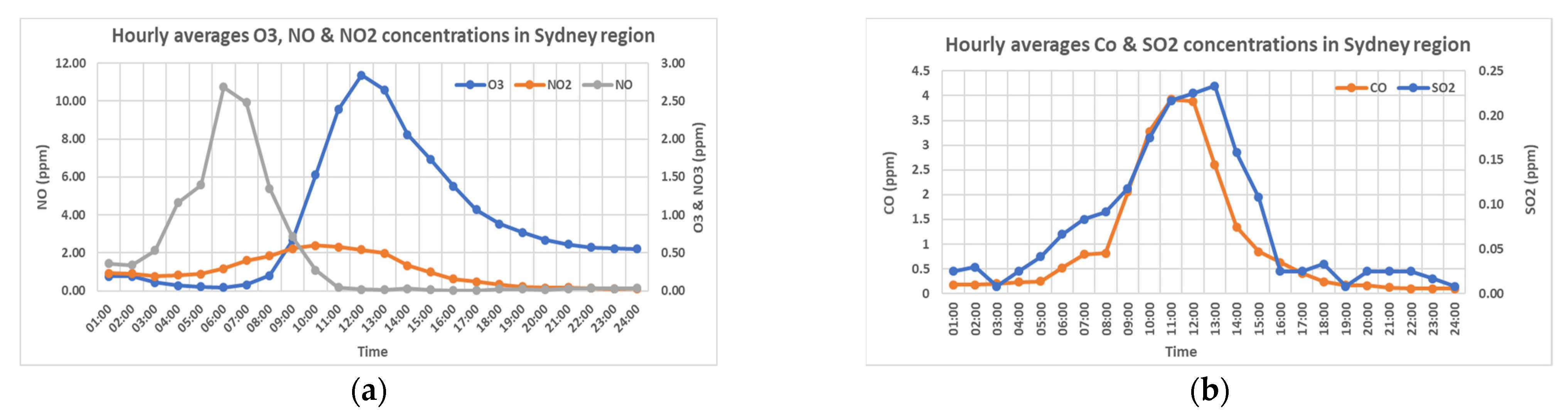
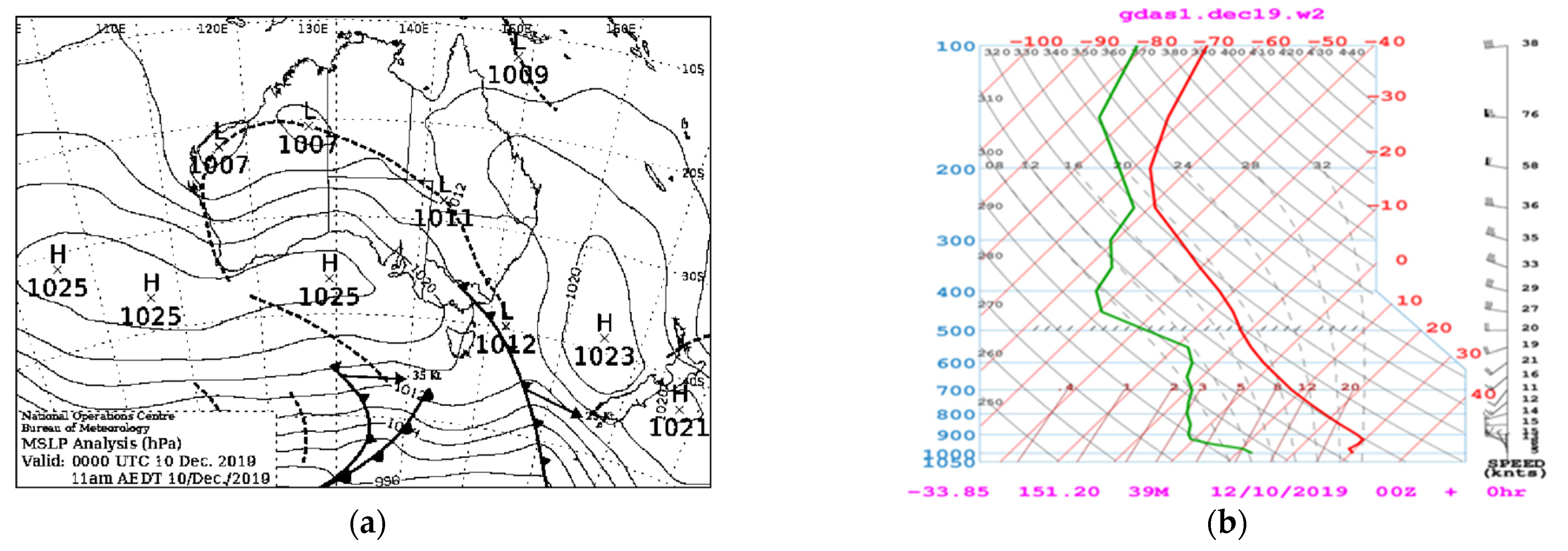
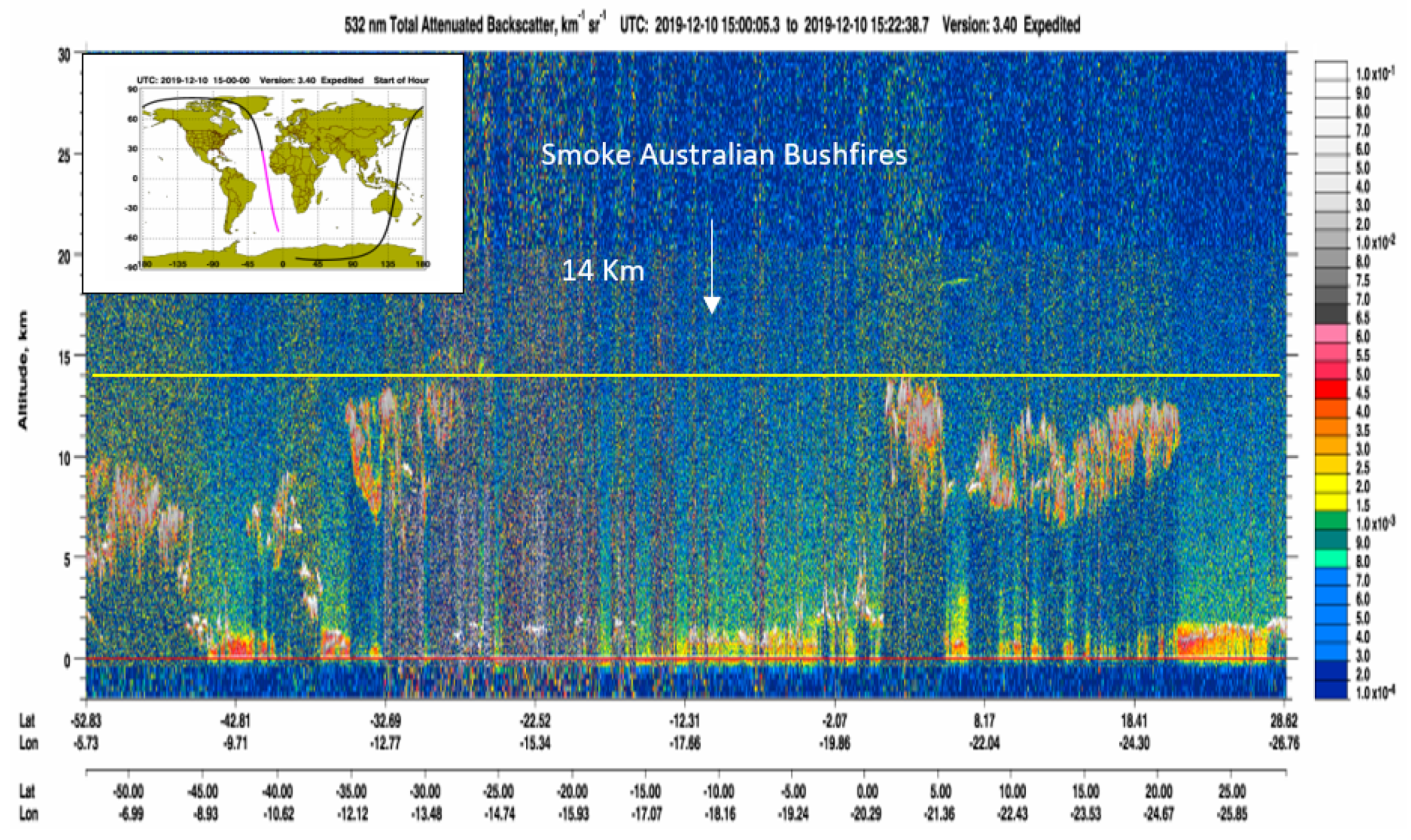
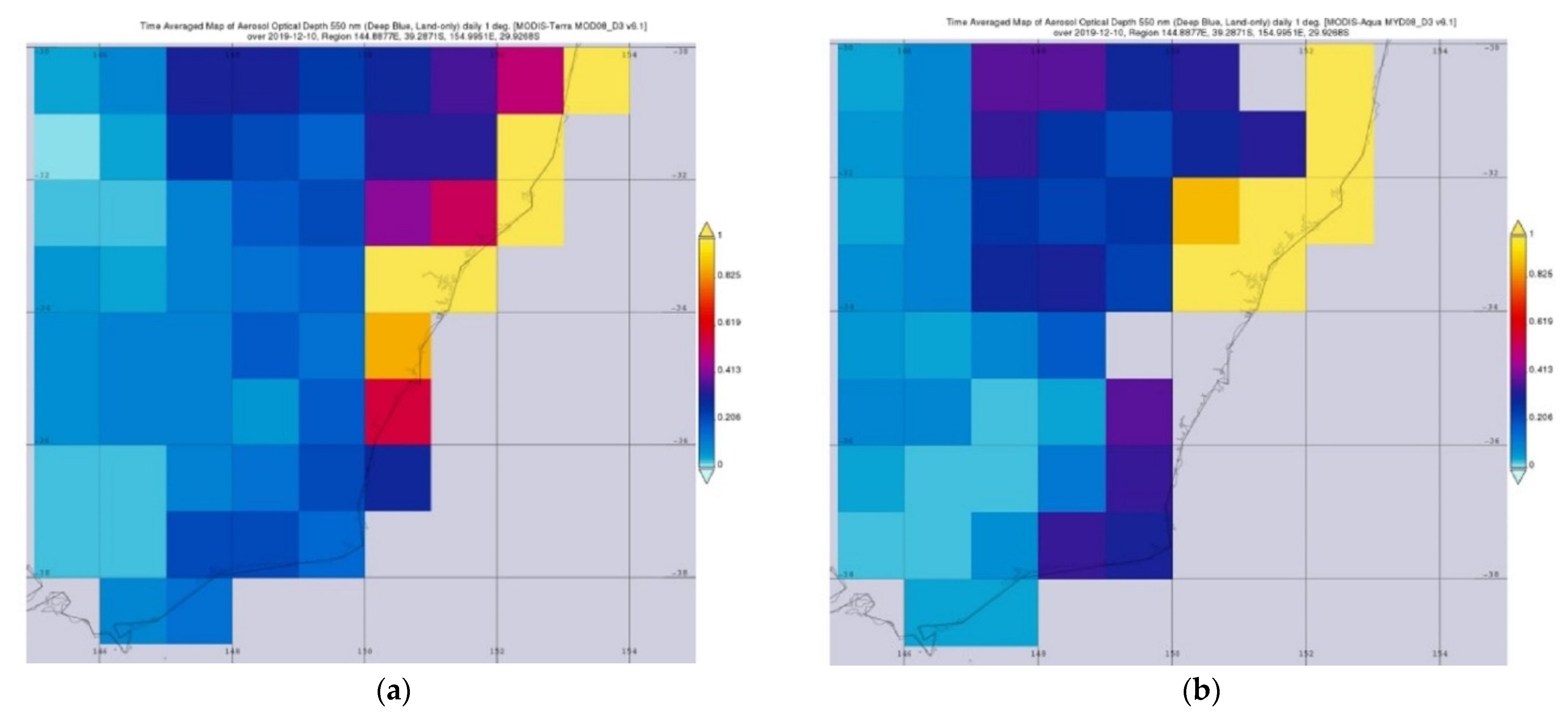
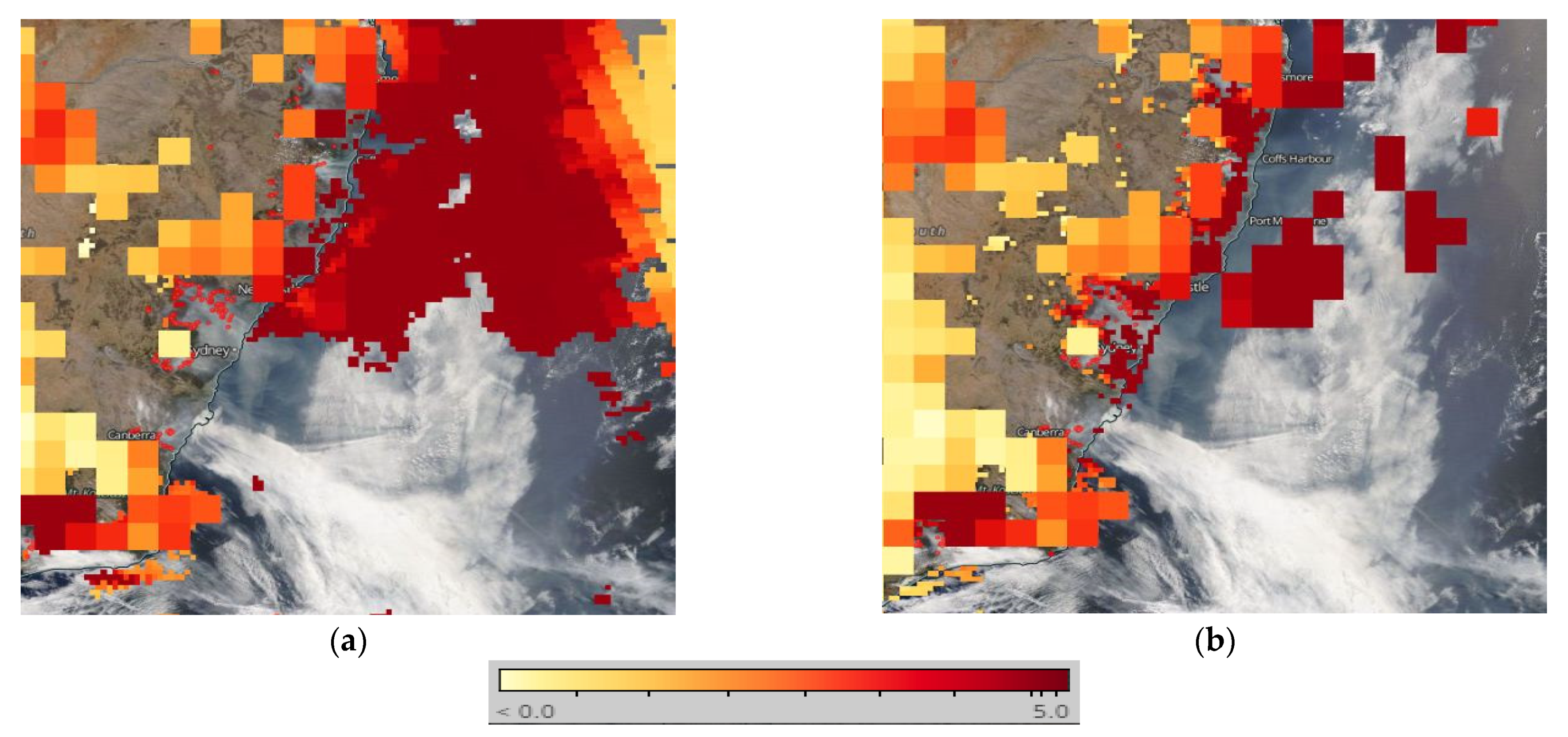
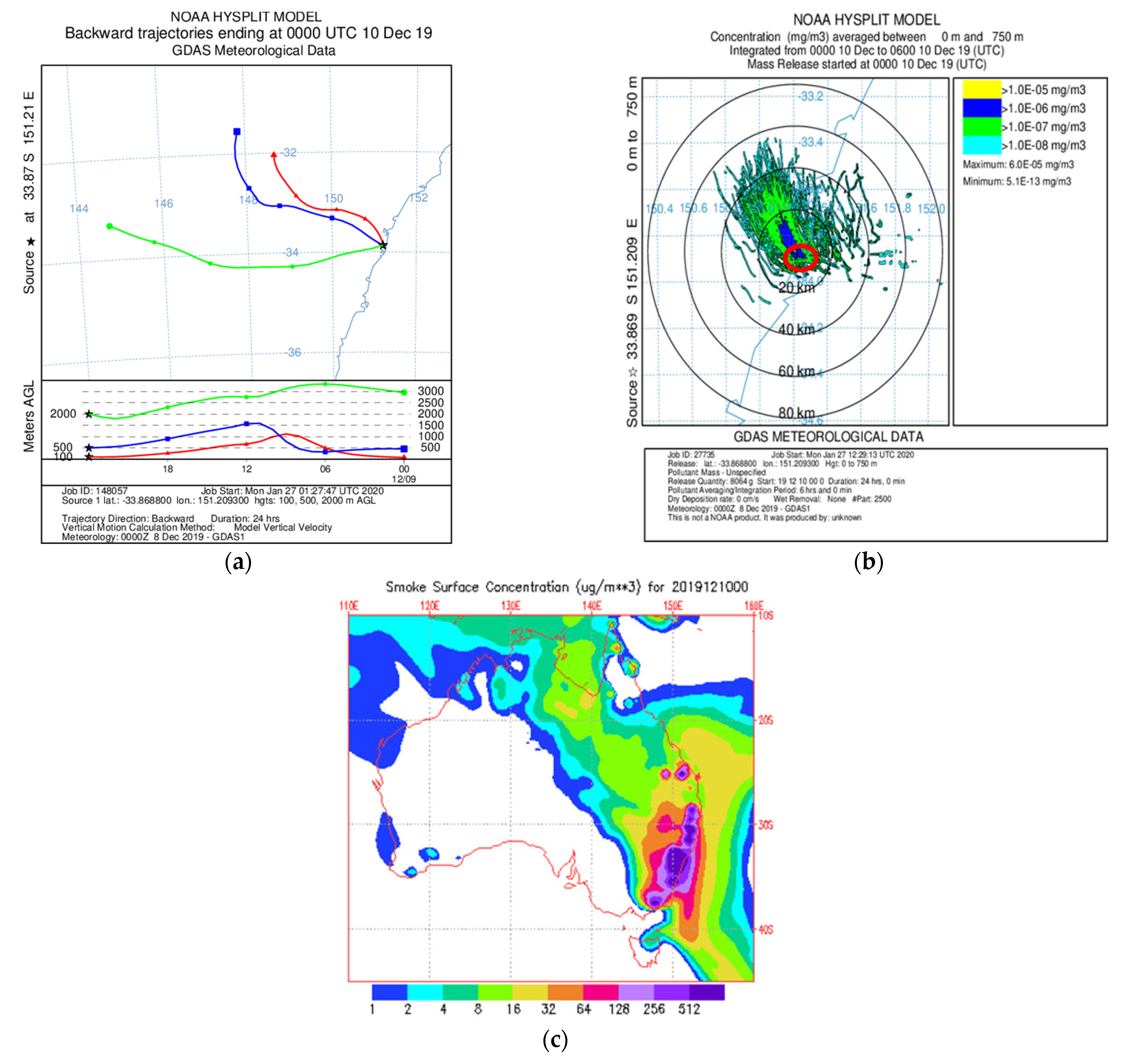
3.2. A Case Study: Bushfire Event on 10 December 2019

An observable decrease in visibility occurred in early December when huge smoke plumes extended over Sydney carrying particulate matter (PM10 & PM2.5) and gases emitted from bushfires. Smoke from the large bushfires in the Blue Mountains area was transported by high winds resulting in increased hourly average particle concentrations between 9–11 December (Figure 4) that were measured by the air quality monitoring network operated by the Office of Environment and Heritage, NSW. Two distinct concentration peaks are apparent. A smaller peak on 9 December is associated with high hourly PM10 concentrations in northwest Sydney (406.9 µg/m3 in St Marys at 14:00 EST) and in southwest Sydney (183.1 μg/m3 in Bringelly at 10:00 EST), while eastern Sydney was less impacted on that day with PM10 concentrations < 75 μg/m3. The second larger peak occurred between 00:00 and 01:00 UTC (11:00–12:00 EST) on 10 December, with high hourly PM10 concentrations recorded in northwest Sydney (929.8 µg/m3 in Prospect and 961.5 µg/m3 in St Marys), wastern Sydney (854.3 μg/m3 in Rozelle at 12:00 EST), and southwest Sydney (729.6 μg/m3 in Liverpool at 13:00 EST).
The Blue Mountains bushfires led to important changes in the gas composition in the atmosphere (Figure 5) caused by the addition of combustion products. On 10 December 2019, the maximum NO concentration was 9.3 ppm in Campbell Town West at 19:00 UTC (06:00 EST). On the same day, the maximum concentration of NO2 was 5.3 ppm in Rozelle, Cook and Phillip at 01:00 UTC (12:00 EST); CO was 5.9 ppm in Macquarie Park at 00:00 UTC (11:00 EST); O3 was 17.9 ppm in Earlwood at 01:00 UTC (12:00 EST); and SO2 was 0.4 ppm in Cook and Phillip at 00:00 UTC (11:00 EST). These concentrations may all be attributed to the bushfires, as they coincide with the increase in PM10 levels recorded during the same period on 10 December 2019. The highest concentrations revealed in the NO values coincide with the lowest O3 values during the study period and may reflect oxidation of the NO to NO2. High O3 values coincided with the highest CO, SO2 and PM10 values and represent the peak influence of bushfire pollutants. The concentrations of SO2 supplied from the air quality monitoring stations over the longer November–December period (Figure 3c) did not indicate an obvious impact of the bushfires for the higher concentrations of this specific gas. Overall, these results indicate the impact of bushfires on at least four of the main pollutants.
On 10 December 2019, the Sydney region was exposed to hot, dry and windy conditions. Surface wind direction was from the west and northwest at 9:00 am and from the south and southeast at 3:00 pm with a maximum wind gust speed of 16.9 m/s, humidity 63–70%, maximum temperature 30.1 °C, pressure 1010.8–1012.9 hPa, and no precipitation. The synoptic chart for 10 December (Figure 6a) displays a deep low-pressure system south of Tasmania, with strong northwesterly winds above the Sydney area ahead of the passage of a frontal system. The vertical temperatures indicated by the Skew-T chart of the soundings in the Sydney area (Figure 6b) suggest a very dry surface layer and a large inversion of temperature at <1000 hPa. The smoke plumes over the Sydney region, related to the huge bushfires in the Blue Mountains and the dominant northwest winds, controlled the boundary layer at this time (Figure 6). This assisted the smoke plume transport to the Pacific Ocean off the east coast of NSW. The synoptic weather conditions (Figure 6a) are consistent with the high-risk fire weather conditions for NSW as advised by the BOM weather service (http://www.bom.gov.au/weather-services/fire-weather-centre/bushfire-weather/index.shtml (accessed on 15 January 2020)).
Australian bushfires are very extreme, and they have lifted smoke plumes all the way up to the stratosphere layer, something bushfires do only sometimes. Radiative heating from soot particles within the smoke makes bushfire smoke plumes especially buoyant, meaning they can reach elevations in the stratosphere layer and stay there longer than material from a volcanic eruption that reaches the same initial height. The National Institute of Aerospace at NASA Langley Research Centre has been using the CALIPSO satellite data to determine the elevation of smoke plumes. The CALIPSO trajectory on 10 December 2019 moved over the borders between South Australia, NSW and Queensland to the Coral Sea off Cairns (Figure 7). The 532 nm total attenuated backscatter signal in Figure 7 detected the existence of an aerosol layer at an elevation of 14 km lying above cirrus stratocumulus clouds at 5–15 km.
The distributions of aerosol optical depth (AOD) from the Aqua and Terra sensors on the MODIS satellite are shown on Figure 8. On 10 December, the maximum aerosol values appeared over the Greater Sydney region, Hunter Valley, Illawarra, northern NSW and southeast Queensland coastal areas, and also above the Pacific Ocean off the coast of Sydney (Figure 8a). Minimum aerosol values were present over the south coast of NSW and northeast Victoria on the same day (Figure 8b).
The smoke distribution can be revealed by the combined AOD values from Aqua and Terra sensors on the MODIS satellite for 10 December 2019 (Figure 9). The regions of greatly elevated aerosol values, suggested by the increased AOD, are present over the Pacific Ocean off Sydney and Newcastle (east coast of NSW), as well as in the Blue Mountains area northwest of Sydney (Figure 9).
The 24 h backward trajectories from HYSPLIT, using the GDAS global data, were started from Sydney at 00:00 UTC (11:00 EST) on 10 December 2019 when the highest hourly concentrations of PM10 occurred within the Sydney region (Figure 3a). The HYSPLIT backward pathways were calculated for 100 m, 500 m and 2000 m above ground level, and are illustrated in red, blue and green lines in Figure 10a. The 100 m and 500 m pathways from Sydney show the direct impact of bushfires from the Blue Mountains causing the very elevated concentrations of PM10 recorded in Sydney and on the east coast of Australia. The HYSPLIT backward pathways also verify the dominant north to northwest winds in the lower boundary layer above Sydney. The 2000 m pathway from Sydney suggest particle transport by the strong west wind at this level. In addition, the HYSPLIT dispersion model indicates that the smoke plume travelled from the northwest at ground level to an elevation of 750 m on 10 December 2019 covering the whole Sydney region (Figure 10b). The NAAPS Aerosol Model also displays the existence of smoke at ground level on 10 December 2019 (Figure 10c).
Periodic changes of the air parcel trajectories towards the western part of NSW during easterly winds was the reason why the smoke plumes did not reach the Sydney region on some days, and the concentrations of air pollutants declined and the subsidence inversion disappeared in the lower atmosphere layer.
The present research depended on the use of combined satellite measurements and ground surface observations (meteorological and air quality data) to interpret the movement of smoke pollutants in the Sydney region. Satellite remote sensing measurements supply high spatial resolution and a larger spatial distribution, while ground surface data provide higher temporal-resolution observations. To link the satellite remote sensing measurements with the ground surface air quality data, air quality and atmospheric modelling tools were applied to either quantitate or increase the understanding of factors that influence air pollutant transport [26]. The current research has used various data to validate the results from the simulation of transport and dispersion modelling tools to understand the influence of bushfires in northern NSW and the Blue Mountains. Different air quality and meteorological models (e.g., HYSPLIT models) were applied to increase knowledge of the correlation between source influences.

4. Discussion

Smoke from the large bushfires in NSW was transported by high winds resulting in increased hourly concentrations of PM10 and PM2.5 in the Sydney area. Three main PM peaks occurred in Sydney in November and December 2019. A more detailed study of the largest peak in December showed a bimodal pattern with two distinct PM10 concentration peaks. A smaller peak on 9 December, had high PM10 values in northwestern and southwestern Sydney, while the eastern part was less impacted on that day. The second peak occurred on 10 December, with high hourly concentrations of PM10 over most of Sydney. Similar findings from around the world indicate that bushfires have a clear influence on PM10 and PM2.5 concentrations [11,39,40,41]. The emitted smoke plumes, especially PM concentrations, during bushfires days also cause a decline in solar radiation.
The 9–11 December bushfires in the Blue Mountains responsible for the smoke in this study also led to important changes in the gas levels in the atmosphere. For example, there was a significant increase in NO concentrations before the arrival of the main PM peak, and it corresponded to the lowest O3 values. The NOx (NO+NO2) emissions during bushfires are related to perfect combustion during the biomass burning stage [42] but the high NO values early in the day may reflect a cooler combustion phase. The decrease in the O3 concentration suggests that direct oxidation of NO into NO2 may have occurred. A similar decline in the O3 concentration due to NO oxidation during bushfire episodes was recorded in the Amazon rainforests [43], while Amiridis et al. [40] recorded a decrease in O3 concentrations as NOx concentrations increased in the smoke aerosols from bushfires. The highest concentrations of NOx, O3 and CO correspond with the highest PM10 values during 10 December and can be attributed to the bushfire smoke While the concentration of SO2 supplied from the air quality monitoring stations also increased on 10 December (Figure 5b), the longer term SO2 concentrations (Figure 3c) did not indicate an obvious impact of the bushfires on this specific gas. Thus, the results show the impact of bushfires on the main pollutants.
A daily average drop in the tropospheric O3 concentration (from 36 to 11 ppb) may be caused by smoke causing a decline in solar radiation and slowing the formation of O3 via photocatalytic operations in the lower troposphere layer [44] or by indirect chemical reactions of gases emitted during bushfires [45]. A study of intercontinental air pollutant transport from the huge 2003 Siberian bushfires and their effect on O3 and CO over large areas of western North America was based on a global chemical transport model (GEOS-CHEM) driven by emission observations from the Global Fire Monitoring Centre (GFMC), trajectories from the HYSPLIT model, AOD measurements from the MODIS satellite, and ground observations (air quality monitoring data) [46]. They found the bushfires led to the air quality levels (O3) being exceeded in the Pacific Northwest region. Impact of long distance ozone transport on ozone concentrations in the northern South China Sea has also been examined using the Pennsylvania State University/National Centre for Atmospheric Research Mesoscale Model Version 5 (PSU/NCAR MM5) together with ground data from air quality monitoring stations [47].
Another method to evaluate the influence of bushfires or biomass burnings on air quality levels is to apply a regional air quality model include atmospheric model and bushfires emission measurements. The Community Air Quality Modelling System (CMAQ), taken from the Weather Research and Forecasting (WRF) model based on National Centre for Environmental Prediction (NCEP) utilising the global final analyses datasets, was used to examine the influence of biomass burning on air quality level in Southeast Asia region and beyond [48]. Satellite and ground surface measurements were used to validate this model. Emission observations from anthropogenic biomass burnings were determined from Intercontinental Chemical Transport Experiment Phase B (INTEXT-B) by NASA in 2006. The biogenic emissions were based on the model of emissions of gases and aerosols from nature (MEGAN) and the fire locating and monitoring of burning emission (FLAMBE).
According to weather observations on 10 December 2019, the Sydney region was hot and dry with strong west and northwest winds and low humidity. The synoptic analyses displayed a deep low-pressure system south of Tasmania causing the northwest winds above Sydney ahead of the passage of a frontal system. The vertical temperatures shown by the Skew-T chart suggest a highly dry surface layer and a large inversion layer at <1000 hPa. CALIPSO satellite data for the same day showed the existence of smoke aerosols above NSW and Queensland with smoke plumes reaching elevations of 14 km. Bushfires rarely lift smoke plumes to these levels. Similar air pollutant transport resulting from Southeast Asia biomass burnings were examined by applying HYSPLIT and WRF models with ground surface observations and MODIS-CALIPSO satellite measurements [49]. Ground, surface micro pulse LIDAR (MPL) and CALIPSO data were applied to monitor the vertical distribution and transport of dust aerosols in Asia from the Gobi and Taklamakan deserts. They identified transported dust aerosols from the Gobi and Taklamakan deserts above the western Pacific Ocean and eastern China by analysing the vertical structure of aerosols from CALIPSO measurements that were in agreement with backward trajectory analyses of air parcels from the HYSPLIT model [50].
The analysis of aerosol optical depth (AOD) using MODIS Aqua and Terra satellites showed the maximum aerosol values were over the Greater Sydney region, Hunter Valley, Illawarra, coastal areas of northern NSW and southeast Queensland, and also above the Pacific Ocean off the coast of Sydney; in contrast, minimum values occurred over the south coast of NSW and northeast Victoria. In a similar manner, Ou-Yang et al. [47] applied the Taiwan air quality model (TAQM) as a chemical atmospheric transport model. Transport of air pollutants, such as gases, dust and aerosols from various sources over Southeast Asia and East Asia has been studied using aerosol loading measurements from ground data with the aerosol robotic network (AERONET) and aerosol measurements from CALIPSO and Terra/Aqua-MODIS satellites [26].
The HYSPLIT backward pathways confirm that the predominant west to northwest winds in the lower boundary layer were responsible for moving the smoke into the Sydney area on 10 December 2019. The lower elevation pathways at 100 m and 500 m were more effective compared to the 2000 m pathway and transported the atmospheric pollutants from the Blue Mountain bushfires to Sydney and out over the Pacific Ocean. The HYSPLIT model backward trajectories confirm the smoke plumes went directly to the Sydney region after the formation of smoke plumes. The findings and approach applied in the current research on smoke aerosol transport (air pollutants) by wildfires follow from similar past research on the influence of bushfires and biomass burnings in different areas around the globe. For example, the long-range air pollutants transport of Southeast Asian biomass burning and their impact on air quality levels in Taiwan have been studied to detect hot spots by using satellite remote sensing observations and the trajectory analysis of air parcels by the HYSPLIT model combined with surface measurements by air quality monitoring stations [51].
The present research has depended on the use of combined satellite measurements and ground surface observations (meteorological and air quality data) to provide the best data interpretations. Satellite remote sensing measurements supply high spatial resolution and a larger spatial distribution, while ground surface data provide higher temporal-resolution observations. To link the satellite remote sensing measurements with the ground surface data requires the application of air quality data and atmospheric modelling tools to either quantitate or increase understand of the influence of air pollutant transport [26].

5. Conclusions

The characteristics of the smoke aerosols, the level of air quality and meteorological data in combination with remote sensing satellite measurements from November and December 2019 were analysed to determine the influence of extensive bushfires in the Sydney area, NSW, Australia.
On 10 December, smoke from the large bushfires in NSW was transported by high winds resulting in increased hourly concentrations of the main air pollutants in the Sydney area. The levels of PM10, PM2.5, NO, NO2, O3, CO determined from air quality measurement stations were all positively correlated with the major bushfire smoke plumes transported over Sydney. The concentrations of SO2 did not indicate an consistent impact from the bushfires for this specific gas. All the maximum PM and gas values were well above the 24 h standard levels for air quality in Australia and thus represent considerable health risks.
The analyses of aerosol measurements from Terra/Aqua-MODIS satellites confirmed that the maximum aerosol values over the Greater Sydney region correlated well with PM measurements, while minimum values occurred away from bushfire areas over the south coast of NSW and northeast Victoria. The remote sensed satellite data supply high spatial resolution and a large spatial distribution for the aerosol transport pathways. Aerosol measurements from CALIPSO showed the existence of smoke aerosols above NSW and Queensland at elevations of up to 14 km while the NAAPS Aerosol Model indicated the existence of smoke at ground level.
Transport pathways can be predicted from synoptic charts and can be confirmed using HYSPLIT back trajectory simulations of air parcels. The latter showed that the predominate west to northwest winds in the lower boundary layer above the Sydney area transported the smoke plumes directly from the Blue Mountains to the Sydney region. Thus, this study provided information on the characteristics and transport of smoke aerosols and to understand their potential impacts on the level of air quality in the Sydney area.
This study recommends the government and researchers use a wide combination of methods to evaluate the influence of bushfires or biomass burnings on air quality levels. There is a need to apply a regional air quality model, including both atmospheric models and bushfires emission measurements, to assess the implications and hazards associated with bushfires emissions. In addition, using ground-based lidar data from AERONET stations to provide good temporal and vertical spatial resolution and aerosol identification could be studied in the future.

Author Contributions

A.A.A.: conceptualisation, methodology, data preparation and processing, data analysis, writing—original draft preparation. B.G.J.: writing—reviewing, language editing, supervision and project administration. All authors have read and agreed to the published version of the manuscript.

Funding

This project has not received funding.

Data Availability Statement

Data available on request from the authors.

Acknowledgments

The authors wish to thank the University of Wollongong and the Bureau of Meteorology (BOM) in Australia for their assistance whenever needed. The provision of air quality monitoring station measurements from the Office of Environment and Heritage is gratefully acknowledged. The authors gratefully acknowledge the NOAA Air Resources Laboratory (ARL) for provision of visualisations and analyses from several satellite remote sensing techniques, such as the HYSPLIT Dispersion and Transport Models through the READY website (http://www.ready.noaa.gov (accessed on 1 January 2020)), the NASA Langley Research Centre through the website http://www-calipso.larc.nasa.gov/products/lidar/browse_images/production/. AOD was obtained from the Giovanni online data system (http://gdata1.sci.gsfc.nasa.gov/ (accessed on 20 January 2020), https://worldview.earthdata.nasa.gov (accessed on 20 January 2020)) and the NAAPS Model from the https://www.nrlmry.navy.mil/aerosol/ website (accessed on 1 January 2020).

Conflicts of Interest

The authors declare no conflict of interest.

References

  1. Duan, F.; Liu, X.; Yu, T.; Cachier, H. Identification and estimate of biomass burning contribution to the urban aerosol organic carbon concentrations in Beijing. Atmos. Environ. 2004, 38, 1275–1282. [Google Scholar] [CrossRef]
  2. Carrico, C.M.; Kreidenweis, S.M.; Malm, W.C.; Day, D.E.; Lee, T.; Carrillo, J.; McMeeking, G.R.; Collett, J.L., Jr. Hygroscopic growth behavior of a carbon-dominated aerosol in Yosemite National Park. Atmos. Environ. 2005, 39, 1393–1404. [Google Scholar] [CrossRef]
  3. Van der Linden, P.; Xiaosu, D. Contribution of Working Group I to the Third Assessment Report of the Intergovernmental Panel on Climate Change; Cambridge University: Cambridge, UK, 2001. [Google Scholar]
  4. Stocker, T.F.; Qin, D.; Plattner, G.-K.; Tignor, M.; Allen, S.K.; Boschung, J.; Nauels, A.; Xia, Y.; Bex, V.; Midgley, P.M. Climate change 2013: The physical science basis. In Contribution of Working Group I to the Fifth Assessment Report of the Intergovernmental Panel on Climate Change; Cambridge University Press: Cambridge, UK, 2013; p. 1535. [Google Scholar]
  5. Williams, R.J.; Gill, A.M.; Bradstock, R.A. Flammable Australia: Fire Regimes, Biodiversity and Ecosystems in A Changing World; CSIRO Publishing: Clayton, Australia, 2012. [Google Scholar]
  6. Scholes, R.; Ward, D.; Justice, C. Emissions of trace gases and aerosol particles due to vegetation burning in southern hemisphere Africa. J. Geophys. Res. Atmos. 1996, 101, 23677–23682. [Google Scholar] [CrossRef]
  7. Levine, J.S. Biomass Burning and Global Change: Remote Sensing, Modeling and Inventory Development, and Biomass Burning in Africa; MIT Press: Cambridge, MA, USA, 1996; Volume 1. [Google Scholar]
  8. Yamasoe, M.A.; Artaxo, P.; Miguel, A.H.; Allen, A.G. Chemical composition of aerosol particles from direct emissions of vegetation fires in the Amazon Basin: Water-soluble species and trace elements. Atmos. Environ. 2000, 34, 1641–1653. [Google Scholar] [CrossRef]
  9. Sinha, P.; Hobbs, P.V.; Yokelson, R.J.; Bertschi, I.T.; Blake, D.R.; Simpson, I.J.; Gao, S.; Kirchstetter, T.W.; Novakov, T. Emissions of trace gases and particles from savanna fires in southern Africa. J. Geophys. Res. Atmos. 2003, 108, D138487. [Google Scholar] [CrossRef]
  10. Andreae, M.O.; Merlet, P. Emission of trace gases and aerosols from biomass burning. Glob. Biogeochem. Cycles 2001, 15, 955–966. [Google Scholar] [CrossRef] [Green Version]
  11. Alves, C.; Gonçalves, C.; Pio, C.; Mirante, F.; Caseiro, A.; Tarelho, L.; Freitas, M.; Viegas, D. Smoke emissions from biomass burning in a Mediterranean shrubland. Atmos. Environ. 2010, 44, 3024–3033. [Google Scholar] [CrossRef]
  12. Crompton, R.P.; McAneney, K.J.; Chen, K.; Pielke Jr, R.A.; Haynes, K. Influence of location, population, and climate on building damage and fatalities due to Australian bushfire: 1925–2009. Weather. Clim. Soc. 2010, 2, 300–310. [Google Scholar] [CrossRef] [Green Version]
  13. Whittaker, J.; Haynes, K.; Handmer, J.; McLennan, J. Community safety during the 2009 Australian ‘Black Saturday’bushfires: An analysis of household preparedness and response. Int. J. Wildland Fire 2013, 22, 841–849. [Google Scholar] [CrossRef] [Green Version]
  14. Reid, J.S.; Eck, T.F.; Christopher, S.A.; Koppmann, R.; Dubovik, O.; Eleuterio, D.; Holben, B.N.; Reid, E.A.; Zhang, J. A review of biomass burning emissions part III: Intensive optical properties of biomass burning particles. Atmos. Chem. Phys. 2005, 5, 827–849. [Google Scholar] [CrossRef]
  15. Adler, G.; Flores, J.; Riziq, A.A.; Borrmann, S.; Rudich, Y. Chemical, physical, and optical evolution of biomass burning aerosols: A case study. Atmos. Chem. Phys. 2011, 11, 1491. [Google Scholar] [CrossRef] [Green Version]
  16. Kasischke, E.S.; Bruhwiler, L.P. Emissions of carbon dioxide, carbon monoxide, and methane from boreal forest fires in 1998. J. Geophys. Res. Atmos. 2002, 107, FFR 2-1–FFR 2-14. [Google Scholar] [CrossRef] [Green Version]
  17. Morgan, G.; Sheppeard, V.; Khalaj, B.; Ayyar, A.; Lincoln, D.; Jalaludin, B.; Beard, J.; Corbett, S.; Lumley, T. Effects of bushfire smoke on daily mortality and hospital admissions in Sydney, Australia. Epidemiology 2010, 21, 47–55. [Google Scholar] [CrossRef]
  18. Johnston, F.; Hanigan, I.; Henderson, S.; Morgan, G.; Bowman, D. Extreme air pollution events from bushfires and dust storms and their association with mortality in Sydney, Australia 1994–2007. Environ. Res. 2011, 111, 811–816. [Google Scholar] [CrossRef]
  19. Le, G.E.; Breysse, P.N.; McDermott, A.; Eftim, S.E.; Geyh, A.; Berman, J.D.; Curriero, F.C. Canadian forest fires and the effects of long-range transboundary air pollution on hospitalizations among the elderly. ISPRS Int. J. Geo-Inf. 2014, 3, 713–731. [Google Scholar]
  20. Guo, Y.; Feng, N.; Christopher, S.A.; Kang, P.; Zhan, F.B.; Hong, S. Satellite remote sensing of fine particulate matter (PM2.5) air quality over Beijing using MODIS. Int. J. Remote Sens. 2014, 35, 6522–6544. [Google Scholar] [CrossRef]
  21. Gupta, P.; Khan, M.N.; da Silva, A.; Patadia, F. MODIS aerosol optical depth observations over urban areas in Pakistan: Quantity and quality of the data for air quality monitoring. Atmos. Pollut. Res. 2013, 4, 43–52. [Google Scholar] [CrossRef] [Green Version]
  22. Carslaw, K.; Boucher, O.; Spracklen, D.; Mann, G.; Rae, J.; Woodward, S.; Kulmala, M. A review of natural aerosol interactions and feedbacks within the Earth system. Atmos. Chem. Phys. 2010, 10, 1701–1737. [Google Scholar] [CrossRef] [Green Version]
  23. Forster, P.; Ramaswamy, V.; Artaxo, P.; Berntsen, T.; Betts, R.; Fahey, D.W.; Haywood, J.; Lean, J.; Lowe, D.C.; Myhre, G. Changes in atmospheric constituents and in radiative forcing. Chapter 2. In Climate Change 2007: The Physical Science Basis; Contribution of Working Group I to the Fourth Assessment Report of the Intergovernmental Panel on Climate Change; Cambridge University: Cambridge, UK, 2007. [Google Scholar]
  24. Toll, V.; Reis, K.; Ots, R.; Kaasik, M.; Männik, A.; Prank, M.; Sofiev, M. SILAM and MACC reanalysis aerosol data used for simulating the aerosol direct radiative effect with the NWP model HARMONIE for summer 2010 wildfire case in Russia. Atmos. Environ. 2015, 121, 75–85. [Google Scholar]
  25. Pere, J.-C.; Mallet, M.; Pont, V.; Bessagnet, B. Impact of aerosol direct radiative forcing on the radiative budget, surface heat fluxes, and atmospheric dynamics during the heat wave of summer 2003 over western Europe: A modeling study. J. Geophys. Res. Atmos. 2011, 116, D23119. [Google Scholar] [CrossRef]
  26. Tsay, S.-C.; Hsu, N.C.; Lau, W.K.-M.; Li, C.; Gabriel, P.M.; Ji, Q.; Holben, B.N.; Welton, E.J.; Nguyen, A.X.; Janjai, S. From BASE-ASIA toward 7-SEAS: A satellite-surface perspective of boreal spring biomass-burning aerosols and clouds in Southeast Asia. Atmos. Environ. 2013, 78, 20–34. [Google Scholar]
  27. Holben, B.N.; Eck, T.F.; Slutsker, I.a.; Tanre, D.; Buis, J.; Setzer, A.; Vermote, E.; Reagan, J.A.; Kaufman, Y.; Nakajima, T. AERONET—A federated instrument network and data archive for aerosol characterization. Remote Sens. Environ. 1998, 66, 1–16. [Google Scholar] [CrossRef]
  28. Pope, C.A., III. Epidemiological basis for particulate air pollution health standards. Aerosol. Sci. Technol. 2000, 32, 4–14. [Google Scholar]
  29. Badarinath, K.; Latha, K.M.; Chand, T.K.; Gupta, P.K.; Ghosh, A.; Jain, S.; Gera, B.; Singh, R.; Sarkar, A.; Singh, N. Characterization of aerosols from biomass burning––A case study from Mizoram (Northeast), India. Chemosphere 2004, 54, 167–175. [Google Scholar] [CrossRef]
  30. Oberdörster, G.; Oberdörster, E.; Oberdörster, J. Nanotoxicology: An emerging discipline evolving from studies of ultrafine particles. Environ. Health Perspect. 2005, 113, 823–839. [Google Scholar]
  31. Löndahl, J.; Swietlicki, E.; Pagels, J.; Massling, A.; Boman, C.; Rissler, J.; Blomberg, A.; Sandström, T. Respiratory tract deposition of particles from biomass combustion. J. Phys. Conf. Ser. 2009, 151, 012066. [Google Scholar] [CrossRef]
  32. Anderson, T.L.; Wu, Y.; Chu, D.A.; Schmid, B.; Redemann, J.; Dubovik, O. Testing the MODIS satellite retrieval of aerosol fine-mode fraction. J. Geophys. Res. Atmos. 2005, 110, D18204. [Google Scholar] [CrossRef] [Green Version]
  33. Draxler, R.R.; Ginoux, P.; Stein, A.F. An empirically derived emission algorithm for wind-blown dust. J. Geophys. Res. Atmos. 2010, 115, D16212. [Google Scholar]
  34. Stein, A.; Draxler, R.R.; Rolph, G.D.; Stunder, B.J.; Cohen, M.; Ngan, F. NOAA’s HYSPLIT atmospheric transport and dispersion modeling system. Bull. Am. Meteorol. Soc. 2015, 96, 2059–2077. [Google Scholar]
  35. Draxler, R.; Rolph, G. HYSPLIT (HYbrid Single-Particle Lagrangian Integrated Trajectory) Model access via NOAA ARL READY Website; Silver Spring: Montgomery, MD, USA; NOAA Air Resources Laboratory: College Park, MD, USA, 2013. Available online: http://ready.arl.noaa.gov/HYSPLIT.php (accessed on 1 January 2020).
  36. Rolph, G. Real-Time Environmental Applications and Display System (READY) Website. 2003. Available online: http://www.arl.noaa.gov/ready.php (accessed on 1 January 2020).
  37. Rolph, G.D.; Draxler, R.R.; Stein, A.F.; Taylor, A.; Ruminski, M.G.; Kondragunta, S.; Zeng, J.; Huang, H.-C.; Manikin, G.; McQueen, J.T. Description and verification of the NOAA smoke forecasting system: The 2007 fire season. Weather. Forecast. 2009, 24, 361–378. [Google Scholar] [CrossRef]
  38. Christensen, J.H. The Danish Eulerian hemispheric model—A three-dimensional air pollution model used for the Arctic. Atmos. Environ. 1997, 31, 4169–4191. [Google Scholar] [CrossRef]
  39. Barnaba, F.; Angelini, F.; Curci, G.; Gobbi, G.P. An important fingerprint of wildfires on the European aerosol load. Atmos. Chem. Phys. 2011, 11, 10487–10501. [Google Scholar]
  40. Amiridis, V.; Zerefos, C.; Kazadzis, S.; Gerasopoulos, E.; Eleftheratos, K.; Vrekoussis, M.; Stohl, A.; Mamouri, R.-E.; Kokkalis, P.; Papayannis, A. Impact of the 2009 Attica wild fires on the air quality in urban Athens. Atmos. Environ. 2012, 46, 536–544. [Google Scholar] [CrossRef]
  41. Saarikoski, S.; Sillanpää, M.; Sofiev, M.; Timonen, H.; Saarnio, K.; Teinilä, K.; Karppinen, A.; Kukkonen, J.; Hillamo, R. Chemical composition of aerosols during a major biomass burning episode over northern Europe in spring 2006: Experimental and modelling assessments. Atmos. Environ. 2007, 41, 3577–3589. [Google Scholar] [CrossRef]
  42. Amaral, S.S.; de Carvalho Junior, J.A.; Costa, M.A.M.; Neto, T.G.S.; Dellani, R.; Leite, L.H.S. Comparative study for hardwood and softwood forest biomass: Chemical characterization, combustion phases and gas and particulate matter emissions. Bioresour. Technol. 2014, 164, 55–63. [Google Scholar] [PubMed]
  43. Rissler, J.; Swietlicki, E.; Zhou, J.; Roberts, G.; Andreae, M.O.; Gatti, L.; Artaxo, P. Physical properties of the sub-micrometer aerosol over the Amazon rain forest during the wet-to-dry season transition? Comparison of modeled and measured CCN concentrations. Atmos. Chem. Phys. 2004, 4, 2119–2143. [Google Scholar]
  44. Deng, X.; Tie, X.; Zhou, X.; Wu, D.; Zhong, L.; Tan, H.; Li, F.; Huang, X.; Bi, X.; Deng, T. Effects of Southeast Asia biomass burning on aerosols and ozone concentrations over the Pearl River Delta (PRD) region. Atmos. Environ. 2008, 42, 8493–8501. [Google Scholar] [CrossRef]
  45. Liu, H.; Chang, W.L.; Oltmans, S.J.; Chan, L.Y.; Harris, J.M. On springtime high ozone events in the lower troposphere from Southeast Asian biomass burning. Atmos. Environ. 1999, 33, 2403–2410. [Google Scholar]
  46. Jaffe, D.; Bertschi, I.; Jaeglé, L.; Novelli, P.; Reid, J.S.; Tanimoto, H.; Vingarzan, R.; Westphal, D.L. Long–range transport of Siberian biomass burning emissions and impact on surface ozone in western North America. Geophys. Res. Lett. 2004, 31, L16106. [Google Scholar]
  47. Ou-Yang, C.-F.; Hsieh, H.-C.; Wang, S.-H.; Lin, N.-H.; Lee, C.-T.; Sheu, G.-R.; Wang, J.-L. Influence of Asian continental outflow on the regional background ozone level in northern South China Sea. Atmos. Environ. 2013, 78, 144–153. [Google Scholar] [CrossRef]
  48. Huang, K.; Fu, J.S.; Hsu, N.C.; Gao, Y.; Dong, X.; Tsay, S.-C.; Lam, Y.F. Impact assessment of biomass burning on air quality in Southeast and East Asia during BASE-ASIA. Atmos. Environ. 2013, 78, 291–302. [Google Scholar] [CrossRef]
  49. Duc, H.N.; Bang, H.Q.; Quang, N.X. Modelling and prediction of air pollutant transport during the 2014 biomass burning and forest fires in peninsular Southeast Asia. Environ. Monit. Assess. 2016, 188, 106. [Google Scholar] [CrossRef]
  50. Huang, J.; Minnis, P.; Chen, B.; Huang, Z.; Liu, Z.; Zhao, Q.; Yi, Y.; Ayers, J.K. Long–range transport and vertical structure of Asian dust from CALIPSO and surface measurements during PACDEX. J. Geophys. Res. Atmos. 2008, 113, D23212. [Google Scholar] [CrossRef]
  51. Yen, M.-C.; Peng, C.-M.; Chen, T.-C.; Chen, C.-S.; Lin, N.-H.; Tzeng, R.-Y.; Lee, Y.-A.; Lin, C.-C. Climate and weather characteristics in association with the active fires in northern Southeast Asia and spring air pollution in Taiwan during 2010 7-SEAS/Dongsha Experiment. Atmos. Environ. 2013, 78, 35–50. [Google Scholar] [CrossRef]
Figure 1. Image from NASA (Aqua and Terra-MODIS satellites) of the huge 10 December 2019 smoke plumes from large NSW bushfires (red dots) that extended along eastern NSW from southern Queensland to south of Canberra.
Remotesensing 14 05552 g001
Figure 2. The locations of air quality monitoring stations in the Sydney area (yellow pins) were plotted on a map using an ArcGIS program to explain their spatial distributions.
Remotesensing 14 05552 g002
Figure 3. Daily maximum concentrations of (a) PM10, PM2.5, (b) NO, NO2, O3, and (c) CO and SO2 measured at air quality monitoring stations in the Sydney region during November and December 2019.
Remotesensing 14 05552 g003
Figure 4. The EST hourly concentration of PM10 recorded by air quality monitoring stations in (a) northwestern, (b) eastern, and (c) southwestern Sydney region between 9 and 11 December 2019. The station locations are shown on Figure 2.
Remotesensing 14 05552 g004
Figure 5. The EST hourly average (a) NO, NO2, O3, and (b) CO, and SO2 concentrations measured at the air quality monitoring stations in Sydney region on 10 December 2019.
Remotesensing 14 05552 g005
Figure 6. (a) Synoptic chart showing isobars (hPa) and frontal systems at 00:00 UTC on 10 December 2019; and (b) Skew-T-log-p diagram for the soundings taken in the Sydney region at the same time. (http://www.bom.gov.au/australia/charts/archive/index.shtml (accessed on 15 January 2020)).
Remotesensing 14 05552 g006
Figure 7. Aerosols measured during the CALIOP daytime transect (inset from [−52.83, −5.73] to [28.75, 26.80]) on 10 December 2019 showing the 532 nm total attenuated backscatter that can distinguish the presence of smoke in the atmosphere.
Remotesensing 14 05552 g007
Figure 8. (a) AOD as measured at 550 nm by the Terra sensor, and (b) the Aqua sensor on the MODIS satellite on 10 December 2019 (https://giovanni.gsfc.nasa.gov/giovanni/ (accessed on 20 January 2020)).
Remotesensing 14 05552 g008
Figure 9. Elevated aerosol values (red) are indicated by the aerosol optical depth (AOD) from the (a) Aqua and (b) Terra sensors on the MODIS satellite. Sites of high bushfire activity (red dots) on 10 December 2019 are also indicated. (https://worldview.earthdata.nasa.gov (accessed on 20 January 2020)).
Remotesensing 14 05552 g009
Figure 10. (a) The 24 h backward trajectories from the HYSPLIT model were calculated over Sydney at 100 m, 500 m and 2000 m above ground level for 10 December 2019 at 00:00 UTC. (b) The HYSPLIT dispersion model was used to determine the 24 h smoke plume dispersion from the bushfires in the Blue Mountains around Sydney for 10 December 2019 at 00:00 UTC. The centre of the red circle is the city of Sydney. (c) Surface smoke concentrations (μg/m3) obtained from the NAAPS Aerosol Model for 10 December 2019.
Remotesensing 14 05552 g010
Table 1. Maximum hourly average pollutant loadings at selected sites in the Sydney region caused by the 2019–2020 Blue Mountains bushfires. UTC = Coordinated Universal Time; EST = Australian Eastern Standard Time.
DateLocationPollutantValueUTCEST
12 NovemberRichmondPM10785 μg/m307:0018:00
26 NovemberRichmondPM10848.9 μg/m307:0018:00
10 DecemberSt MarysPM10961.5 μg/m301:0012:00
12 NovemberRandwickPM10466.5 μg/m307:0018:00
26 NovemberRandwickPM10575.3 μg/m307:0018:00
10 DecemberRandwickPM10197.7 μg/m322:0009:00
12 NovemberChulloraPM2.5103.4 μg/m315:0002:00
26 NovemberRouse HillPM2.5162.7 μg/m322:0009:00
10 DecemberOakdalePM2.5714.6 μg/m318:0005:00
19 NovemberParramatta NorthNO18.2 ppm19:0006:00
10 DecemberRouse HillO33.3 ppm06:0017:00
19 DecemberRandwickO39.8 ppm00:0011:00
10 DecemberMacquarie ParkCO5.9 ppm00:0011:00
29 NovemberRandwickSO21.4 ppm23:0010:00
21 DecemberRozelleSO21.7 ppm00:0011:00
Publisher’s Note: MDPI stays neutral with regard to jurisdictional claims in published maps and institutional affiliations.

