
Identifying the Influencing Factors of Cooling Effect of Urban Blue Infrastructure Using the Geodetector Model
1
School of Forestry and Landscape Architecture, Anhui Agricultural University, Hefei 230036, China
2
Hefei National Urban Ecosystem Research Station, Hefei 230036, China
3
School of Environmental and Geographical Sciences, Shanghai Normal University, Shanghai 200234, China
4
Yangtze River Delta Urban Wetland Ecosystem National Field Scientific Observation and Research Station, Shanghai 200234, China
5
School of Art and Design, Dalian Polytechnic University, Dalian 116000, China
*
Author to whom correspondence should be addressed.
Remote Sens. 2022, 14(21), 5495; https://doi.org/10.3390/rs14215495
Submission received: 1 October 2022
/
Revised: 22 October 2022
/
Accepted: 29 October 2022
/
Published: 31 October 2022
(This article belongs to the Special Issue Remote Sensing in Applied Ecology)
Abstract
:The urban heat island (UHI) effect has a serious negative impact on urban ecosystems and human well-being. Mitigating UHI through nature-based methods is highly recommended. The cooling effect of urban blue infrastructure (UBI) can significantly alleviate the effects of UHI. Revealing the crucial influencing factors of the cooling effect of UBI is of great significance for mitigating the UHI effect. In this study, the water-cooling intensity (WCI) and water-cooling range (WCR) were used to quantitatively analyze the cooling effect of UBI in Hefei city in summer. Furthermore, the influencing factors and their interactions with the cooling effect of UBI were investigated based on the Geodetector model. The results revealed that: (1) The surface thermal environment of the built-up area of Hefei presented obvious spatial differentiation characteristics. (2) There were nine influencing factors that significantly influenced the WCI variation, with the greatest influencing factor of road density. In contrast, only the landscape shape index had a significant effect on WCR variation. (3) The interaction of environmental characteristics, water body characteristics, and socioeconomic characteristics had a significant influence on the cooling effect of UBI, and the interaction relationship between the influencing factors was mutually enhanced. The findings from our research can provide a theoretical reference and practical guidance for the protection, restoration, and planning of UBI as a nature-based solution to improve the urban thermal environment.
1. Introduction
As the global urbanization process continues to accelerate, a large number of people are flocking to cities. Urban areas are facing increasing challenges due to rapid urbanization and climate change. Urbanization has significantly transformed natural surfaces into impervious surfaces, which alters the materials, energy, radiation, and composition of the atmospheric structure in the near-surface layer [1]. Changes in underlying urban surfaces and frequent human activities have an impact on the processes and services of natural ecosystems, resulting in a series of social and ecological problems [2,3]. The urban heat island (UHI) effect is one of the best-documented urbanization-related environmental problems and presents a variety of challenges for people, including decreasing environmental quality, injuring human health, increasing energy consumption, and jeopardizing the region’s sustainable development [4,5,6]. Consequently, alleviating the UHI effect has become one of the key research topics at present, and mitigating associated negative effects in natural ways is considered an environmentally friendly and politically and socially acceptable approach [7,8].
Urban Blue Infrastructure (UBI) and Urban Green Infrastructure (UGI) are all critical natural landscapes in mitigating the UHI effect [9,10,11,12]. However, most of the research focuses on UGI’s cooling effect [13,14]. UBI includes artificial or natural water bodies, such as rushing water bodies (e.g., rivers, creeks, and canals) and stilling water bodies (e.g., lakes, ponds, wetlands, reservoirs, and seashore lines) [15]. The cooling effect of UBI is a result of its innate characteristics and its interaction with the state of the surrounding environment [14]. Compared with other natural surfaces, water bodies are an ideal thermal radiation absorber, as it has high thermal inertia and storage, low heat conductivity, and brightness [16]. Notably, UBI can provide a remarkable cooling effect on areas close to the water [17,18,19], and compared to the seasonal variation of UGI, the cooling effect of UBI is more stable [20,21]. Furthermore, compared to green spaces, water bodies can deliver a greater cooling effect [13,14,15,16,17,18,19,20]. Therefore, a deeper understanding of the cooling effect of water bodies and its impact factors can enhance the current insights into the adaptation strategies for UHI effects [13,22,23].
The cooling range and cooling intensity of water bodies in different regions have been investigated and identified [9,18,21,24,25,26]. Additionally, there is increasing attention focusing on the influencing factors of water bodies cooling effect [18,27,28,29,30]. Statistical methods, such as principal component analysis [31,32], linear regression analyses [33,34,35], stepwise multiple-linear regression [36,37], and ordinary least-squares regression (OLS) [38], have been widely used in the investigation of influencing factors using multiple variables. However, most of the statistical approaches are based on the linear-based hypothesis, which cannot be used to adequately measure factors influencing the spatial heterogeneity of the UBI cooling effect in a nonlinear way. Considering that the cooling effect of UBI is usually influenced by multiple influencing factors, the above methods are based on the linear assumption, and difficult to deal with the combined effects. Based on spatial hierarchical heterogeneity, the Geodetector model is a statistical approach, and its core idea is based on the assumption that if an independent variable has an important influence on a dependent variable, the spatial distribution of the independent variable and the dependent variable should be similar. The principle is to analyze the relationship between the within-strata variance and the total variance of each factor and use spatial stratified heterogeneity to detect the influencing force of each factor on the dependent variable. The key advantages of this model are that it has fewer assumptions than the statistical methods mentioned above, and the results are not impacted by the collinearity of several variables. Second, this model is also capable of detecting the comprehensive contribution of two factors interacting with the dependent variable [39,40]. The Geodetector has been extensively utilized to examine the driving force in public health [39,40,41], regional economics [42,43], meteorology [44,45], and land use fields [46,47]. Considering that the cooling effect of water body is affected by multiple factors and the interaction between them is extremely complex, it is difficult to fully measure the internal mechanism by using the linear hypothesis. Therefore, this research attempts to explore the application of the Geodetector model to investigate the driving mechanisms of the cooling effect of UBI.
This paper takes Hefei, the capital city of Anhui province, as a case study region. Hefei, an essence city in central China, has experienced a pronounced summertime UHI effect in recent years [48]. The study aims to investigate the relationship between UBI and land surface temperature (LST), estimate the cooling effects of UBI on the thermal environment in summer, and investigate the influence of natural and socioeconomic factors on UBI cooling effects. This study focuses on the following two questions: (1) What are the cooling intensity and cooling range of UBI? (2) What are the crucial influencing factors of the UBI cooling effect and their interactions? This study is helpful in offering a theoretical reference and practical guidance for the protection, planning, and design of UBI for moderating the UHI effect.
2. Materials and Methods
2.1. Study Area
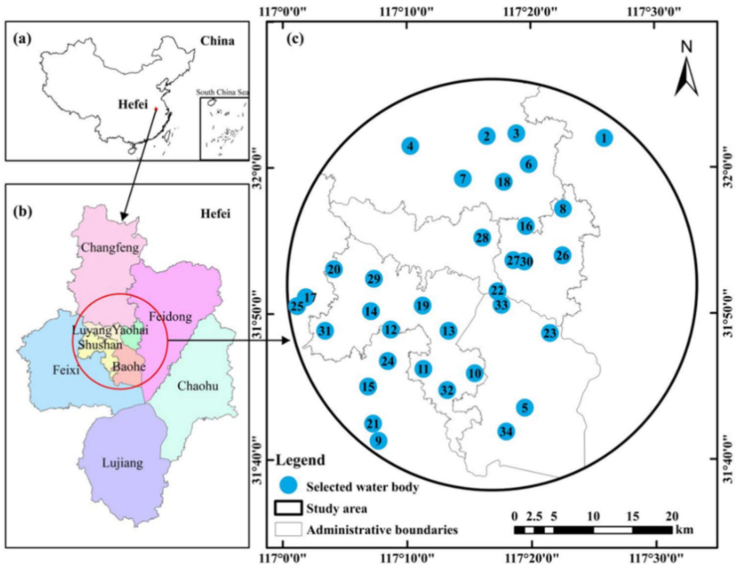
Hefei (30°56′N~32°32′N, 116°40′E~117°58′E) is in the center of Anhui Province between the Yangtze River and the Huai River. With elevation ranges from 12 to 45 m, the average elevation is 30 m. The region has a northern subtropical humid monsoon climate, and the climate variation is characterized by mild spring and autumn, chilly winter, and scorching summer. Based on the long-term records, the average yearly temperature is 15.7 °C [48]. The summer months of late June through early September have higher temperature and the winter months of December through the following February has a lower temperature. Winter has the lowest temperature, at about −20.6 °C, and summer has the highest temperature, around 41 °C. The precipitation in Hefei is about 1000 mm, most of which occurs from June to August in summer, then the spring and autumn, and the least during the winter. The four seasons, from spring to winter, account for 25%, 44%, 20%, and 11% of the total annual precipitation, respectively. Hefei is a key city of the ‘Rise of central China’ strategy, with an area of 11,445 km2. At the end of 2020, the number of permanent resident citizens increased to 9.37 million, while the urbanization rate rose to 76.33% (Hefei Bureau of Statistics, http://tjj.hefei.gov.cn/). The rapid urbanization, high-density construction area areas, and high-intensity economic activities have led to unusually high summer temperatures in Hefei, and the UHI effect is severe in summer [48,49]. The intense UHI effect has seriously affected people’s normal life and urban operation, so it is representative and practical to study the cooling effect of urban blue infrastructure in this region. Therefore, the major urban area of Hefei was chosen as the research place (Figure 1), including four municipal districts (Shushan, Baohe, Yaohai, and Luyang district) and parts of Feidong county, Feixi county, and Changfeng county.
2.2. Data Collection
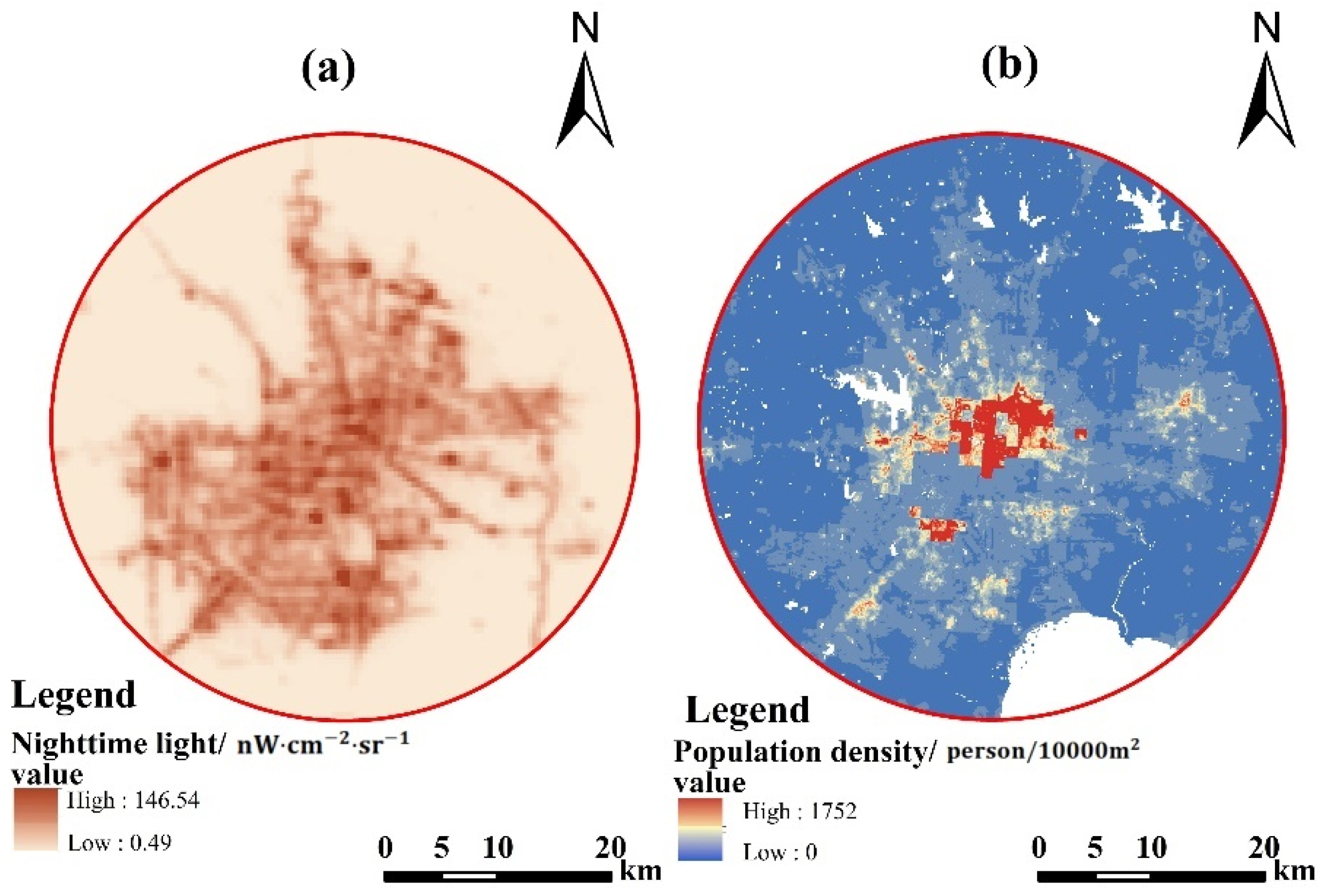
In this study, UBI and LST data were extracted by multi-source remote sensing data in Hefei city. Landsat-8 OLI/TIRS remote sensing images were used for the interpretation and retrieval of land cover data and LST. Clear sky images (https://earthexplorer.usgs.gov/) (accessed on 15 December 2021) were taken on 14 September 2017, at a spatial resolution of 30 m. Furthermore, the remote sensing data, land use data, and meteorological data covering the study area were also collected and sorted as auxiliary information for LST retrieval. The daily surface temperature data in different periods were obtained from the National Meteorological Science Data Sharing Service Platform (http://data.cma.cn/) (accessed on 1 March 2022). The population density data were provided by Worldpop (https://www.worldpop.org/) (accessed on 20 March 2022). The NPP-VIIRS nighttime light data in September of 2017 (https://www.ngdc.noaa.gov/eog/viirs/download_dnb_composites.html) (accessed on 22 March 2022) were resampled to the spatial resolution of 1 km (https://landscan.ornl.gov/landscan-datasets) (accessed on 10 April 2022) to describe the socioeconomic development level locally (Figure 2).
2.3. Methods
2.3.1. Retrieval of LST
The Radiative Transfer Equation (RTE) method was adopted to retrieve LST using Landsat remote sensing data [50]. The retrieval accuracy of this method has been proven relatively accurate [51], and the accuracy can reach 0.6 °C [52]. The RTE approach can be represented by the apparent radiance Lλ received by the satellite sensor. Then the atmospheric upward radiance (Latm, i↑), atmospheric radiation reaches the ground down after the reflected energy (Latm, i↓) and transmissivity (τ) can be acquired from NASA’s website (http://atmcorr.gsfc.nasa.gov/) (accessed on 1 March 2022) estimated. The luminance value Lλ of thermal infrared radiation received by the satellite sensor can be expressed as the formula (1) [53]:
where ε is the surface-specific emissivity, Ts is the LST, B(Ts) is the blackbody thermal radiance, and τ is the transmittance of the atmosphere in the thermal infrared band. According to Planck’s law, the radiation brightness B(Ts) of a black body at temperature T in the thermal infrared band can be expressed as Equation (2) [54]. Finally, LST can be calculated by Equation (3) [55]:
Lλ = [εB(Ts) + (1 − ε) Latm, i↓]τ + Latm, i↑
B(Ts) = [Lλ − Latm, i↑ − τ(1 − ε) Latm, i↓]/τε
Ts = K2/ln(K1/B(Ts) + 1)
The radiometric calibration tool IDL 8.6 in ENVI 5.3 was used to calibrate the surface radiation image and acquire the 10-band radiation image. For landsat-8 TIRS image band 10, K1 = 774.89 (mW m−2s·r−1 μm−1), K2 = 1321.08 K.
This study used the China Meteorological Data Network (http://data.cma.cn/data/online.html?t=1) (accessed on 10 December 2021) to check the weather in Hefei on the day of the satellite transit. The temperature ranged from 18 °C to 29 °C. On this basis, the accuracy of the retrieved LST is verified. Since the special underlying surface of the city increases the difference between LST and air temperature [56], it can be considered that the inversion results are roughly accurate. Therefore, the retrieved temperature can be used to study the UHI effect in Hefei.
2.3.2. Identification and Selection of Water Bodies
The modified normalized difference water index (MNDWI) [57] was used to delineate UBI. MNDWI is a widely used indicator to distinguish urban water bodies from other land cover types [58,59]. As a fast, simple, and accurate method to extract water information, its principle is to extract water information by analyzing the spectral properties of the water bodies and selecting bands with a high likelihood of water body recognition. The MNDWI was calculated by [30,57]:
MNDWI = (GREEN − MIR)/(GREEN + MIR)
GREEN is a green band, such as band 3 (0.525–0.600 μm) of Landsat OLS image, and MIR is a middle infrared band, such as band 6 (1.560–1.651 μm) of Landsat OLS image. The MNDWI pixel value greater than 0 was considered to belong to the water body.
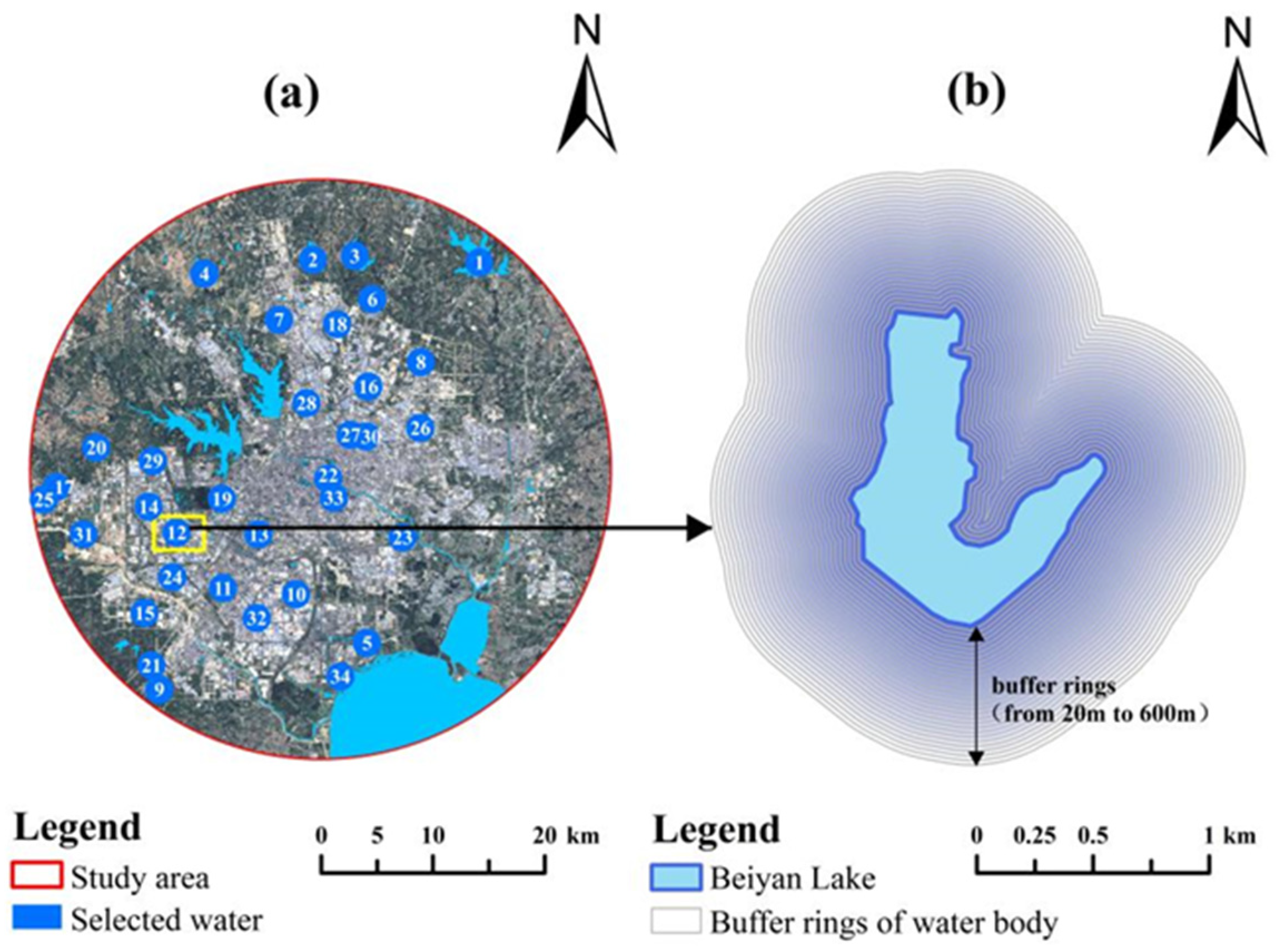
To explore the correlation between UBI and LST and investigate the cooling effect of UBI, water bodies were randomly selected in the study area. To reduce subjectivity, improve analytical reliability, and avoid the influence of the cooling effect produced by two water bodies, the following selection criteria were formulated: (1) a certain number of water bodies were selected by a random selection algorithm in the ArcGIS tool randomly; (2) refer to the other studies [29,60] and actual investigations, the distance between each selected water body should be greater than 600 m, which can be roughly considered that the water bodies will not affect each other; (3) the selected water body should be at least 600 m away from Chaohu Lake. Finally, a total of 34 water bodies in the research region were extracted for investigation, including 5 reservoirs, 24 urban lakes, 2 urban rivers, and 3 urban ponds (Figure 3a).
2.3.3. Quantitative Analysis of the UBI Cooling Effect
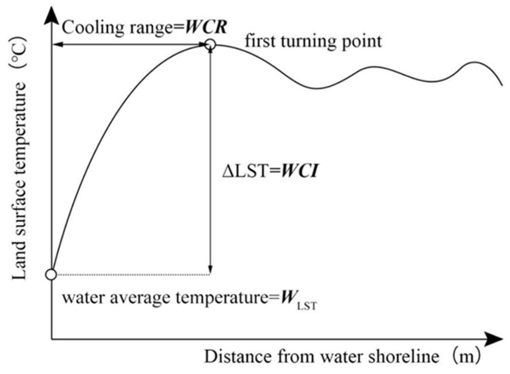
In this research, the cooling intensity and cooling range [13,21] were used to quantify the cooling effect of UBI. Specifically, the cooling intensity means the differences in LST between the water body and its surrounding environment, and the cooling range means the maximum distance a water body can cool. As shown in Figure 4, water LST (WLST) shows the average LST of every selected water body, and water-cooling intensity (WCI) represents the LST variation between the average water body LST and the turning point buffer LST. The water-cooling range (WCR) is defined as the range between a water body and a turning point [21]. According to the boundary of the selected water body, 30 ring-shaped buffers were installed around the selected water bodies, and the radius was increased by 20 m (Figure 3b). Next, it was determined what the average LST values were for each ring buffer and calculated for chosen water bodies. Eventually, the WCI and WCR were determined by the difference in average LST and the range between the turning point buffer and the water bodies [61].
2.3.4. Choosing Potential Influencing Factors
The influencing factors of the UBI cooling effect are highly diverse and complex. Based on previous studies [29,30,60], this study selected 11 potential influencing factors covering three aspects: environmental characteristics, water body characteristics, and socioeconomic development characteristics. Table 1 lists detailed information on influencing factors.
2.3.5. Statistical Analysis
Geodetector was used to investigate the relationship between the UBI cooling effect and influencing factors. Geodetector is a set of statistical methods designed to detect spatial heterogeneity and show the driving forces behind it [62]. Compared with traditional models, it can analyze the relationship between variables based on linear assumptions and collinearity of variables [41,63]. The Geodetector model has been applied to the research range from the natural field to the social field, such as the research on the effects of human activities and ecological factors on urban surface temperature [44], the influencing mechanism of residents’satisfaction with livability [64], the detection of the dominant factors of the spatial variation of continental cleavage degree in the United States [65]. The Geodetector is mainly composed of a factor detector, interaction detector, ecological detector, and risk detector [66,67]. In our study, a factor detector and an interactive detector were used to analyze the influencing factors of spatial differentiation of the UBI cooling effect in Hefei city.
- (1)
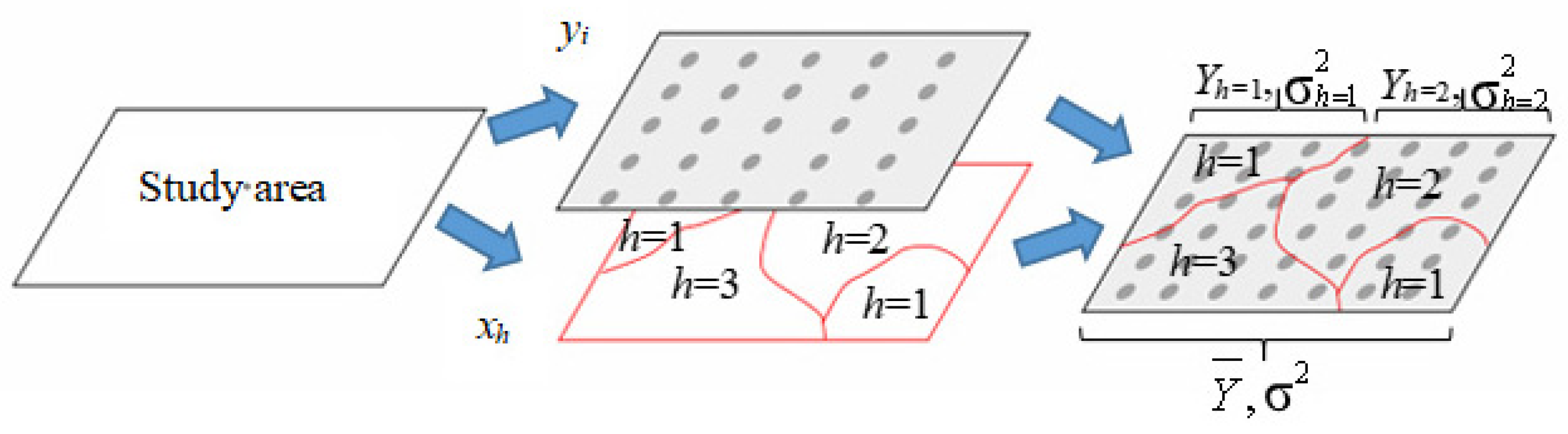
- The factor detector mainly detects to what extent an independent variable (X) explains the spatial variation in the attribute of the dependent variable (Y), and the value is measured by the q value (Figure 5). In this paper, the factor detector was employed to identify the influence of different factors on the spatial variation of the UBI cooling effect. The calculation formula of the q value is [68]:where h = 1, …, L is the layer of impact factor X; Nh and N represent the number of sample units in layer h and the whole region, respectively. and σ2 are the variances of layer h and the variance of the whole region. SSW represents the total of the spatial variance of each layer. SST represents the difference of Y in the whole region. The range of values for q is [0, 1]. The higher the q value, the stronger the explanatory power and contribution of this factor to the spatial differentiation of the UBI cooling effect, and the weaker it is, on the contrary [69,70].
The factor detector analysis can only reflect the influence degree of factors but cannot reflect the positive and negative of the influence [48]. Therefore, the Pearson correlation coefficient was used to represent the positive and negative association between the cooling index and influencing factors in this study [30]. The Pearson correlation coefficient was conducted in SPSS 26.0 software (IBM, Armonk, NY, USA).
- (2)
- The interaction detector is used to determine the interaction between various factors, that is, whether two factors work interact to enhance or diminish the explanatory power of the dependent variable (Y) or whether the effects of such factors on Y are independent of each other, which means the factor’s influence on the UBI cooling effect is likely to be independent and can also be combined. Different from traditional statistical methods, such as logistic regression hypothesis multiplication, interaction detectors can be detected as long as there is interaction [71,72]. The evaluation method is to overlay geography layers X1 and X2 to create a new geography layer Y. Compare the q values of Y, X1, and X2 to judge the effect of the interaction (Table 2) [63].
3. Results
3.1. Spatial Characteristics of UBI and LST
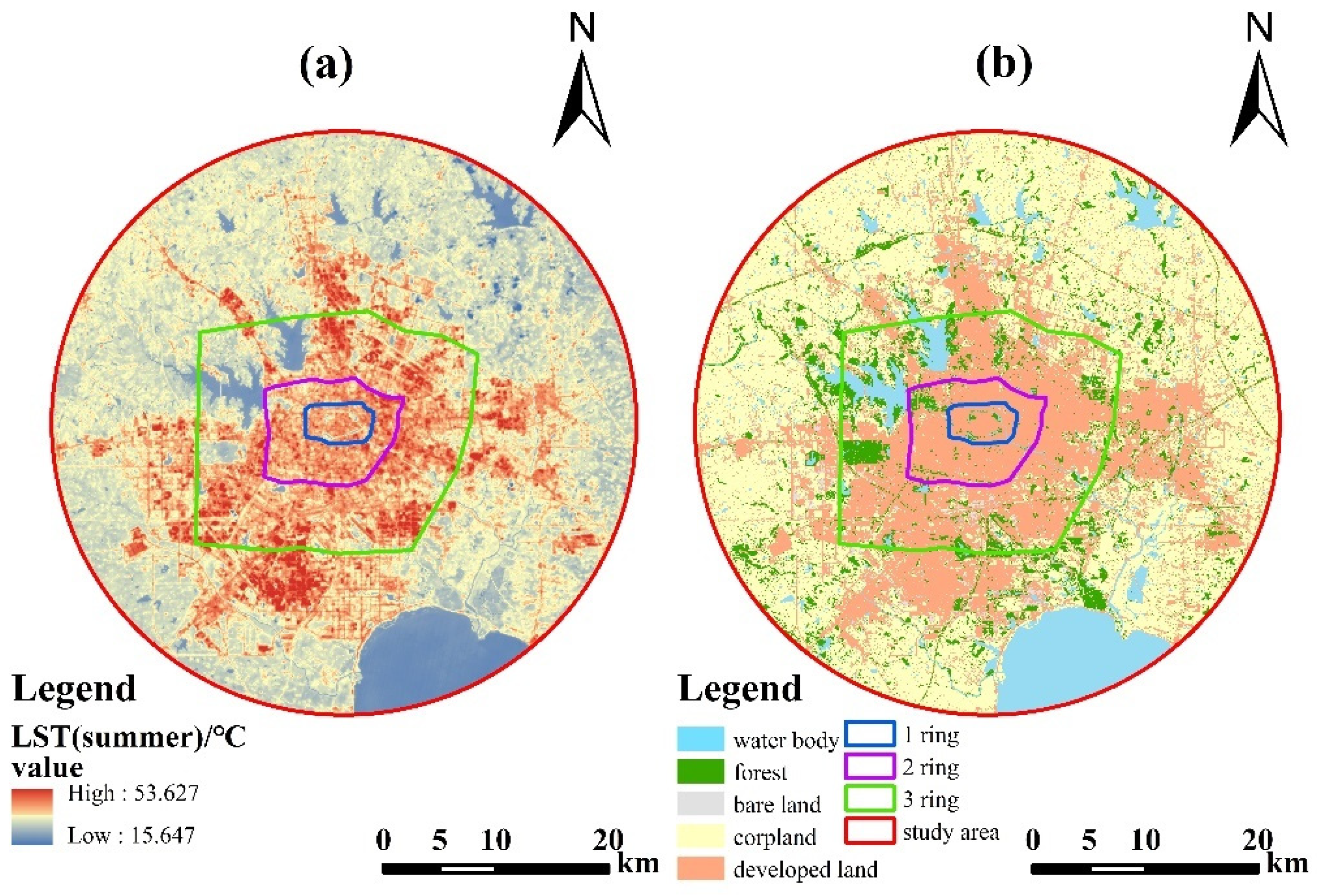
The spatial heterogeneity of LST distribution was obvious (Figure 6a). The LST ranged from 15.65 to 53.63 °C, and the average LST was 31.57 °C in the study area. According to the several city ring roads, the study region was divided into four parts, the core area, the inner ring area, the central area, and the outer ring area. The core area had the characteristics of a high plot ratio and high density of population; however, there was a typical cold island area formed by the ring park, which made the average surface temperature lower than that in the inner ring (Table 3). The inner ring area exhibited the highest average LST. The central area includes both densely developed areas and part of suburban areas, the mean LST in this part was much lower than that in the inner ring area, and it can be clearly seen that two large reservoirs and Shushan Forest Park in the northwest are a typical urban cold island. The outer ring area is dominated by newly developed area, industrial land, large reservoirs, and rural agricultural land. The mean LST in this area is the lowest.
3.2. The Cooling Effect of UBI
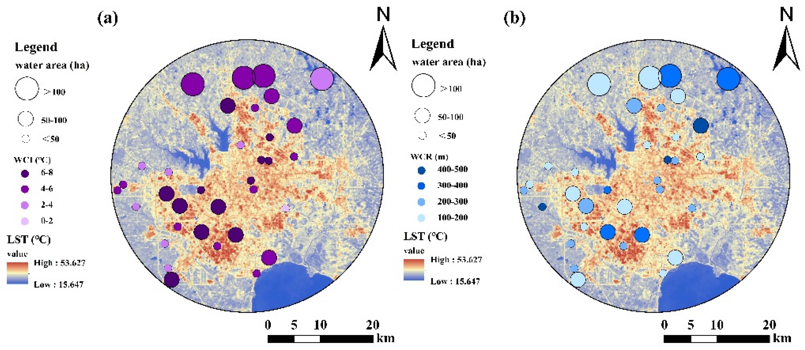
There are 394 water bodies in the study region; the area of the selected 34 water bodies ranged from 3.88 to 875.52 ha, with an average area of 72.62 ha, showing significant differences in area. The WCR ranged from 500 m in Shaoquan Lake to 140 m in Degong Lake, with an average distance of 343.08 m (Figure 7). The average WCR of ponds (300 m) was the furthest, followed by rivers (270 m), urban lakes (239.17 m), and reservoirs (228 m). The average WCI was 5.21 °C, ranging from 7.94 °C in Tanchong Lake to 1.51 °C in Nanfei River. The average WCI of urban lakes (5.67 °C) was the largest, followed by rivers (4.45 °C), reservoirs (3.92 °C), and ponds (3.34 °C).
3.3. Influencing Factor Analysis of UBI Cooling Effect
As shown in Table 4, nine factors passed the significance test (p < 0.05) to explain the WCI variation. In the environmental characteristics layer, the explanatory power of the cooling effect ranged from the water slope (0.260) and the distance of the surrounding water system (0.133) to the water body connectivity (0.119). In the water body characteristics layer, the water patch size (0.340) had higher explanatory power, followed by the water landscape shape index (0.260). In the socioeconomic development characteristics layer, road density (0.359) had the highest explanatory power, which was obviously higher than other factors. By contrast, only the landscape shape index (0.181) passed the significance test (p < 0.05) to explain the WCR variation.
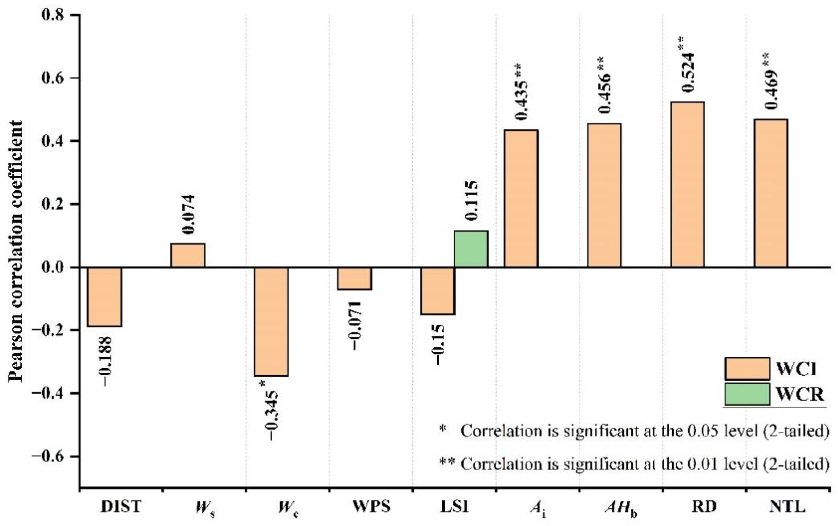
The Pearson correlation coefficients between WCI, WCR, and influencing factors are shown in Figure 8. In the environmental characteristics layer, the WCI of each water body was significantly negatively correlated with Wc (R = −0.345, p < 0.05). The DIST and Ws were negatively and positively correlated with WCI, respectively. In the water body characteristics layer, the WPS and LSI factors were negatively correlated. In the socioeconomic development characteristics layer, all four factors had a significant positive correlation with WCI, of which the most significant was observed for RD (R = 0.524, p < 0.01), followed by NTL (R = 0.469, p < 0.01), AHb (R = 0.456, p < 0.01), and Ai (R = 0.435, p < 0.01). The LSI was the only potential influencing factor for the WCR, and the correlation analysis shows a positive correlation.
In accordance with the interaction detector model, the interaction between influencing factors and cooling indicators (WCI and WCR) was investigated. Our study focused on the interactions between factors from various layers rather than within the very same level. The results indicated that the interaction between influencing factors was bilinear or nonlinear, and the interaction q value of each join of factors was greater than that of the two factors, indicating that the interaction relationship between influencing factors of the UBI cooling effect was mutually enhanced. The cooling effect of UBI is the result of the incorporated effects of environmental characteristics, water body characteristics, and socioeconomic development characteristics.
The interactive detection analysis results showed (Table 5) that the interactions of water body characteristics and socioeconomic development characteristics had a significant impact on WCI. Specifically, the largest interactions between the factors were WPS∩RD (0.68), Av∩WPS (0.64), WPS∩NTL (0.64), and DIST∩RD (0.62), indicating that the design and location of water bodies have a greater influence on the cooling effect. The interactive detection results of WCR (Table 6) showed that the largest interactions between the factors were Ws∩LSI (0.52), Ai∩WPS (0.38), Ai∩LSI (0.38), and Ws∩AHb (0.38). In particular, the interactions between Ws and the four socioeconomic factors were more than 0.36, although the differences between these interactions were small. There was no denying that the interaction between the characteristics of environmental characteristics and socioeconomic development characteristics was the most significant.
4. Discussion
4.1. The Effects of UBI on LST
In this study, we found that there were obvious spatial differences in UHI, and the LST decreased gradually from the central city to the suburbs of Hefei (Figure 6). This is due to the strong correlation between the urban thermal environment and the urban land use types [73,74,75], among which UBI was one of the key factors in mitigating the UHI effect. Based on the spatial superposition analysis of water bodies and LST, we found that the average water LST corresponding to the core area, inner ring area, central area, and outer ring area were 29.88 °C, 30.06 °C, 29.28 °C, and 27.76 °C, which were 5.18 °C, 5.18 °C, 4.93 °C, and 3.19 °C, lower than the mean LST of each area, respectively. This indicated that the UBI can effectively slow down the rise of the urban LST and become a ‘cold island’ in the urban thermal environment. Compared to urban green infrastructure, the cooling effect of UBI are steadier because it is the best absorber of radiation [30], and the UBI are able to create a stronger cooling effect than urban green infrastructure [60,76]. Meanwhile, due to the high heat capacity and low thermal conductivity, water bodies have the ‘thermostatic effect’ to preserve their original temperature through the cooling effect when the ambient temperature rises [59]. Generally, the larger the water area, the better the cooling effect [77]. In this research, the size of the water body had the strongest explanatory power for cooling intensity except for road density, indicating that the area of urban water played a significant role in the mitigation of the thermal atmosphere, which is consistent with earlier studies [27,30,77].
4.2. Implications for UBI Landscape Planning and Management
With the rapid urbanization process, UHI has become one of the most important environmental issues in the world. The nature-based solutions to mitigate UHI are considered to be the best way [78]. Our study indicated that UBI has an obvious cooling effect on surrounding areas. Urban water areas, especially small-sized water bodies, may be preferentially transformed into other land uses to meet the need for the urban socioeconomic development [79,80,81]. As the key natural landscape type in urban areas, better planning and management of UBI may have significant implications for improving UHI.
Previous studies have shown that socioeconomic development influenced by urbanization was the main influencing factor of UHI [60,72]. Our research indicated the socioeconomic development variables all had strong explanatory power to the cooling effect of UBI and were positively correlated with the WCI, and the RD had the greatest explanatory power. The UBI planning and management should consider not only the old downtown area with dense roads but also the organic combination of road construction and UBI in the new development area. Related studies have proved that the cooling intensity of UBI had a close relationship with the size and shape of water bodies [21,54,76,82]. Our results also showed that patch size and landscape shape index of water bodies had a strong explanatory power on WCI variation. Some researchers argued that it is unrealistic and unsustainable to increase the size of water bodies due to over-urbanized areas often lacking sufficient space [13,54,59,60,83]. Therefore, water bodies with more complicated shapes should be designed during UBI planning, which is of great significance for UHI mitigation.
The interaction between water patch size (WPS) and road density (RD) and nighttime light (NTL) greatly enhanced the interpretation of WCI variation, respectively, which means planning should consider both patch size and local socioeconomic development to improve WCI and mitigate UHI effects. Our research results found that slope, the distance of the surrounding water system, and water connectivity had a great explanatory power, which emphasizes the need to consider the natural environment factors around UBI. Therefore, the UBI planning should consider both water characteristics, such as water size and shape index, regional socioeconomic growth, and the natural environment to efficiently reduce the UHI effect.
Compared with other studies [29,61], our research also found that the LSI of water was the only potential driving factor on WCR. The interactive detection results showed that interaction between water slope (Ws) and landscape shape index (LSI), water slope (Ws), and average building height (AHb) greatly enhanced the interpretation power of WCR respectively, probably because these influencing factors can change the wind speed and trend around the water bodies, thus affecting the WCR. Therefore, the spatial arrangement and geographical location of UBI should be considered to improve the WCR of water bodies.
4.3. Limitations of this Study and Research Directions in the Future
In this paper, we selected the potential influencing factors of the cooling effect of UBI from three aspects, but the internal mechanism of the cooling effect is extremely complex, with numerous influencing factors. Therefore, more factors need to be explored in the future, such as water deepness, volume, and types (rushing water or still water). Furthermore, some exploratory findings on the interaction of the UBI cooling effect have also been summarized in accordance with the interaction detector model; however, the Geodetector model is difficult to be used to finish the calculation of the interaction among three or more factors. Therefore, how to simulate the interactions in increasingly complicated circumstances deserves to be developed in further research.
5. Conclusions
Based on GIS spatial statistics and remote sensing technology, this paper analyzed the cooling effect of UBI in Hefei city using the indices of WCI and WCR. Meanwhile, the Geodetector models were adopted to identify the influencing factors of the cooling effect of blue infrastructure from multiple aspects. The results are as follows:
- (1)
- The surface thermal environment of the built-up area of Hefei presented obvious spatial differentiation characteristics. The high-temperature area was mainly concentrated in the core and inner ring area, while the low-temperature area was mainly distributed in the outer ring area and several large reservoirs and forest parks.
- (2)
- Nine factors have a significant influence on WCI, including DIST, Ws, Wc, WPS, LSI, Ai, AHb, RD, and NTL, among which road density had the highest explanatory power for WCI variation. In contrast, only the landscape shape index had a significant impact on WCR variation.
- (3)
- The cooling effect of UBI is the result of the comprehensive effects of environmental characteristics, water body characteristics, and socioeconomic development characteristics. The interaction of the three type factors had a significant effect on WCI and WCR, and the interaction relationship between the influencing factors was mutually enhanced.
Our results indicate that several factors, such as socioeconomic development and natural environment, have an impact on the cooling effect of UBI. On this basis, it is suggested that future studies should consider more types of UBI and other influencing factors. In conclusion, this study extends our understanding and perception of the cooling effects of UBI, especially the factors that potentially influence the cooling effects of water bodies. These findings can provide suggestions on how to design UBI geographically and spatially to achieve better cooling effects and improve the urban thermal environment, particularly in cities that are undergoing rapid urbanization.
Author Contributions
Conceptualization, Y.L. and R.Z.; methodology, Y.L. and L.H.; software, Y.L. and M.X.; validation, Y.L., R.Z. and Q.M.; formal analysis, Y.L. and D.L.; investigation, Y.L. and M.X.; resources, Y.L. and R.Z.; data curation, Y.L., M.X. and L.H.; writing—original draft preparation, Y.L., R.Z. and Q.M.; writing—review and editing, Y.L. and R.Z.; visualization, Y.L. and M.X.; supervision, R.Z.; project administration, Y.L. and R.Z.; funding acquisition, Y.L. and R.Z. All authors have read and agreed to the published version of the manuscript.
Funding
This study was supported by the National Natural Science Foundation of China (Nos. 32071831 and 41730642), the Humanities and Social Sciences Research Project for Youth Scholars of the Ministry of Education (22YJCZH092), the General Science Foundation of Shanghai Normal University (Nos. SK202256 and SK202155), and the Soft Science Foundation of Shanghai, China (No. 19692108200).
Data Availability Statement
The data that support the findings of this study are available from the corresponding author upon reasonable request.
Acknowledgments
The authors would like to thank the anonymous reviewers for their valuable comments to improve the quality of the paper.
Conflicts of Interest
The authors declare no conflict of interest.
References
- Zhou, R.; Xu, H.; Zhang, H.; Zhang, J.; Liu, M.; He, T.; Gao, J.; Li, C. Quantifying the Relationship between 2D/3D Building Patterns and Land Surface Temperature: Study on the Metropolitan Shanghai. Remote Sens. 2022, 14, 4098. [Google Scholar] [CrossRef]
- Peng, J.; Xie, P.; Liu, Y.; Ma, J. Urban thermal environment dynamics and associated landscape pattern factors: A case study in the Beijing metropolitan region. Remote Sens. Environ. 2016, 173, 145–155. [Google Scholar] [CrossRef]
- Sun, R.; Lu, Y.; Yang, X.; Chen, L. Understanding the variability of urban heat islands from local background climate and urbanization. J. Clean. Prod. 2019, 208, 743–752. [Google Scholar] [CrossRef]
- Akbari, H.; Kolokotsa, D. Three decades of urban heat islands and mitigation technologies research. Energy Build. 2016, 133, 834–842. [Google Scholar] [CrossRef]
- Cao, Q.; Yu, D.; Georgescu, M.; Wu, J.; Wang, W. Impacts of future urban expansion on summer climate and heat-related human health in eastern China. Environ. Int. 2018, 112, 134–146. [Google Scholar] [CrossRef] [PubMed]
- Sun, Y.; Augenbroe, G. Urban heat island effect on energy application studies of office buildings. Energy Build. 2014, 77, 171–179. [Google Scholar] [CrossRef]
- Martins, T.A.L.; Adolphe, L.; Bonhomme, M.; Bonneaud, F.; Faraut, S.; Ginestet, S.; Michel, C.; Guyard, W. Impact of Urban Cool Island measures on outdoor climate and pedestrian comfort: Simulations for a new district of Toulouse, France. Sustain. Cities Soc. 2016, 26, 9–26. [Google Scholar] [CrossRef]
- Nesshover, C.; Assmuth, T.; Irvine, K.N.; Rusch, G.M.; Waylen, K.A.; Delbaere, B.; Haase, D.; Jones-Walters, L.; Keune, H.; Kovacs, E.; et al. The science, policy and practice of nature-based solutions: An interdisciplinary perspective. Sci. Total Environ. 2017, 579, 1215–1227. [Google Scholar] [CrossRef] [PubMed]
- Amani-Beni, M.; Zhang, B.; Xie, G.-D.; Xu, J. Impact of urban park’s tree, grass and waterbody on microclimate in hot summer days: A case study of Olympic Park in Beijing, China. Urban For. Urban Green. 2018, 32, 1–6. [Google Scholar] [CrossRef]
- Moss, J.L.; Doick, K.J.; Smith, S.; Shahrestani, M. Influence of evaporative cooling by urban forests on cooling demand in cities. Urban For. Urban Green. 2019, 37, 65–73. [Google Scholar] [CrossRef]
- Sun, R.; Chen, L. Effects of green space dynamics on urban heat islands: Mitigation and diversification. Ecosyst. Serv. 2017, 23, 38–46. [Google Scholar] [CrossRef]
- Chen, L.; Wang, X.; Cai, X.; Yang, C.; Lu, X. Combined Effects of Artificial Surface and Urban Blue-Green Space on Land Surface Temperature in 28 Major Cities in China. Remote Sens. 2022, 14, 448. [Google Scholar] [CrossRef]
- Yang, G.; Yu, Z.; Jorgensen, G.; Vejre, H. How can urban blue-green space be planned for climate adaption in high-latitude cities? A seasonal perspective. Sustain. Cities Soc. 2020, 53, 101932. [Google Scholar] [CrossRef]
- Gunawardena, K.R.; Wells, M.J.; Kershaw, T. Utilising green and bluespace to mitigate urban heat island intensity. Sci. Total Environ. 2017, 584, 1040–1055. [Google Scholar] [CrossRef] [PubMed]
- Voelker, S.; Baumeister, H.; Classen, T.; Hornberg, C.; Kistemann, T. Evidence for the temperature-mitigating capacity of urban blue space—A health geographic perspective. Erdkunde 2013, 67, 355–371. [Google Scholar] [CrossRef]
- Wilson, J.S.; Clay, M.; Martin, E.; Stuckey, D.; Vedder-Risch, K. Evaluating environmental influences of zoning in urban ecosystems with remote sensing. Remote Sens. Environ. 2003, 86, 303–321. [Google Scholar] [CrossRef]
- Manteghi, G.; Limit, H.B.; Remaz, D. Water Bodies an Urban Microclimate: A Review. Mod. Appl. Sci. 2015, 9, 97. [Google Scholar] [CrossRef] [Green Version]
- Xue, Z.; Hou, G.; Zhang, Z.; Lyu, X.; Jiang, M.; Zou, Y.; Shen, X.; Wang, J.; Liu, X. Quantifying the cooling-effects of urban and peri-urban wetlands using remote sensing data: Case study of cities of Northeast China. Landsc. Urban Plan. 2019, 182, 92–100. [Google Scholar] [CrossRef]
- Zheng, Y.; Li, Y.; Hou, H.; Murayama, Y.; Wang, R.; Hu, T. Quantifying the Cooling Effect and Scale of Large Inner-City Lakes Based on Landscape Patterns: A Case Study of Hangzhou and Nanjing. Remote Sens. 2021, 13, 1526. [Google Scholar] [CrossRef]
- Brans, K.I.; Engelen, J.M.T.; Souffreau, C.; De Meester, L. Urban hot-tubs: Local urbanization has profound effects on average and extreme temperatures in ponds. Landsc. Urban Plan. 2018, 176, 22–29. [Google Scholar] [CrossRef]
- Du, H.; Song, X.; Jiang, H.; Kan, Z.; Wang, Z.; Cai, Y. Research on the cooling island effects of water body: A case study of Shanghai, China. Ecol. Indic. 2016, 67, 31–38. [Google Scholar] [CrossRef]
- Cheng, L.; Guan, D.; Zhou, L.; Zhao, Z.; Zhou, J. Urban cooling island effect of main river on a landscape scale in Chongqing, China. Sustain. Cities Soc. 2019, 47, 101501. [Google Scholar] [CrossRef]
- Mohajerani, A.; Bakaric, J.; Jeffrey-Bailey, T. The urban heat island effect, its causes, and mitigation, with reference to the thermal properties of asphalt concrete. J. Environ. Manag. 2017, 197, 522–538. [Google Scholar] [CrossRef]
- Bouzouidja, R.; Cannavo, P.; Bodenan, P.; Gulyas, A.; Kiss, M.; Kovacs, A.; Bechet, B.; Chancibault, K.; Chantoiseau, E.; Bournet, P.-E.; et al. How to evaluate nature-based solutions performance for microclimate, water and soil management issues—Available tools and methods from Nature4Cities European project results. Ecol. Indic. 2021, 125, 107556. [Google Scholar] [CrossRef]
- Jacobs, C.; Klok, L.; Bruse, M.; Cortesao, J.; Lenzholzer, S.; Kluck, J. Are urban water bodies really cooling? Urban Clim. 2020, 32, 100607. [Google Scholar] [CrossRef]
- Tominaga, Y.; Sato, Y.; Sadohara, S. CFD simulations of the effect of evaporative cooling from water bodies in a micro-scale urban environment: Validation and application studies. Sustain. Cities Soc. 2015, 19, 259–270. [Google Scholar] [CrossRef]
- Tan, X.; Sun, X.; Huang, C.; Yuan, Y.; Hou, D. Comparison of cooling effect between green space and water body. Sustain. Cities Soc. 2021, 67, 102711. [Google Scholar] [CrossRef]
- Wu, J.; Li, C.; Zhang, X.; Zhao, Y.; Liang, J.; Wang, Z. Seasonal variations and main influencing factors of the water cooling islands effect in Shenzhen. Ecol. Indic. 2020, 117, 106699. [Google Scholar] [CrossRef]
- Wu, C.; Li, J.; Wang, C.; Song, C.; Chen, Y.; Finka, M.; La Rosa, D. Understanding the relationship between urban blue infrastructure and land surface temperature. Sci. Total Environ. 2019, 694, 133742. [Google Scholar] [CrossRef]
- Wang, Y.; Ouyang, W. Investigating the heterogeneity of water cooling effect for cooler cities. Sustain. Cities Soc. 2021, 75, 103281. [Google Scholar] [CrossRef]
- Zhou, W.; Huang, G.; Cadenasso, M.L. Does spatial configuration matter? Understanding the effects of land cover pattern on land surface temperature in urban landscapes. Landsc. Urban Plan. 2011, 102, 54–63. [Google Scholar] [CrossRef]
- Weng, Q.; Liu, H.; Liang, B.; Lu, D. The Spatial Variations of Urban Land Surface Temperatures: Pertinent Factors, Zoning Effect, and Seasonal Variability. IEEE J. Sel. Top. Appl. Earth Obs. Remote Sens. 2008, 1, 154–166. [Google Scholar] [CrossRef]
- Chen, A.; Yao, L.; Sun, R.; Chen, L. How many metrics are required to identify the effects of the landscape pattern on land surface temperature? Ecol. Indic. 2014, 45, 424–433. [Google Scholar] [CrossRef]
- Morabito, M.; Crisci, A.; Messeri, A.; Orlandini, S.; Raschi, A.; Maracchi, G.; Munafo, M. The impact of built-up surfaces on land surface temperatures in Italian urban areas. Sci. Total Environ. 2016, 551, 317–326. [Google Scholar] [CrossRef]
- Sun, Q.; Wu, Z.; Tan, J. The relationship between land surface temperature and land use/land cover in Guangzhou, China. Environ. Earth Sci. 2012, 65, 1687–1694. [Google Scholar] [CrossRef]
- Asgarian, A.; Amiri, B.J.; Sakieh, Y. Assessing the effect of green cover spatial patterns on urban land surface temperature using landscape metrics approach. Urban Ecosyst. 2015, 18, 209–222. [Google Scholar] [CrossRef]
- Huang, X.; Wang, Y. Investigating the effects of 3D urban morphology on the surface urban heat island effect in urban functional zones by using high-resolution remote sensing data: A case study of Wuhan, Central China. Isprs J. Photogramm. Remote Sens. 2019, 152, 119–131. [Google Scholar] [CrossRef]
- Peng, J.; Jia, J.; Liu, Y.; Li, H.; Wu, J. Seasonal contrast of the dominant factors for spatial distribution of land surface temperature in urban areas. Remote Sens. Environ. 2018, 215, 255–267. [Google Scholar] [CrossRef]
- Liao, Y.; Wang, J.; Du, W.; Gao, B.; Liu, X.; Chen, G.; Song, X.; Zheng, X. Using Spatial Analysis to Understand the Spatial Heterogeneity of Disability Employment in China. Trans. GIS 2017, 21, 647–660. [Google Scholar] [CrossRef]
- Liao, Y.; Zhang, Y.; He, L.; Wang, J.; Liu, X.; Zhang, N.; Xu, B. Temporal and Spatial Analysis of Neural Tube Defects and Detection of Geographical Factors in Shanxi Province, China. PLoS ONE 2016, 11, e0150332. [Google Scholar] [CrossRef]
- Huang, J.; Wang, J.; Bo, Y.; Xu, C.; Hu, M.; Huang, D. Identification of Health Risks of Hand, Foot and Mouth Disease in China Using the Geographical Detector Technique. Int. J. Environ. Res. Public Health 2014, 11, 3407–3423. [Google Scholar] [CrossRef] [PubMed]
- Tan, J.; Zhang, P.; Lo, K.; Li, J.; Liu, S. The Urban Transition Performance of Resource-Based Cities in Northeast China. Sustainability 2016, 8, 1022. [Google Scholar] [CrossRef] [Green Version]
- Xu, Q.; Zheng, X.; Zhang, C. Quantitative Analysis of the Determinants Influencing Urban Expansion: A Case Study in Beijing, China. Sustainability 2018, 10, 1630. [Google Scholar] [CrossRef] [Green Version]
- Ren, Y.; Deng, L.-Y.; Zuo, S.-D.; Song, X.-D.; Liao, Y.-L.; Xu, C.-D.; Chen, Q.; Hua, L.-Z.; Li, Z.-W. Quantifying the influences of various ecological factors on land surface temperature of urban forests. Environ. Pollut. 2016, 216, 519–529. [Google Scholar] [CrossRef] [Green Version]
- Wu, R.; Zhang, J.; Bao, Y.; Zhang, F. Geographical Detector Model for Influencing Factors of Industrial Sector Carbon Dioxide Emissions in Inner Mongolia, China. Sustainability 2016, 8, 149. [Google Scholar] [CrossRef] [Green Version]
- Ju, H.; Zhang, Z.; Zuo, L.; Wang, J.; Zhang, S.; Wang, X.; Zhao, X. Driving forces and their interactions of built-up land expansion based on the geographical detector—A case study of Beijing, China. Int. J. Geogr. Inf. Sci. 2016, 30, 2188–2207. [Google Scholar] [CrossRef]
- Ren, Y.; Deng, L.; Zuo, S.; Luo, Y.; Shao, G.; Wei, X.; Hua, L.; Yang, Y. Geographical modeling of spatial interaction between human activity and forest connectivity in an urban landscape of southeast China. Landsc. Ecol. 2014, 29, 1741–1758. [Google Scholar] [CrossRef]
- Li, Y.; Liu, Y.; Ranagalage, M.; Zhang, H.; Zhou, R. Examining Land Use/Land Cover Change and the Summertime Surface Urban Heat Island Effect in Fast-Growing Greater Hefei, China: Implications for Sustainable Land Development. ISPRS Int. J. Geo-Inf. 2020, 9, 568. [Google Scholar] [CrossRef]
- Sun, J.; Ongsomwang, S. Impact of Multitemporal Land Use and Land Cover Change on Land Surface Temperature Due to Urbanization in Hefei City, China. ISPRS Int. J. Geo-Inf. 2021, 10, 809. [Google Scholar] [CrossRef]
- Jimenez-Munoz, J.; Sobrino, J.; Skokovic, D.; Mattar, C.; Cristobal, J. Land Surface Temperature Retrieval Methods from Landsat-8 Thermal Infrared Sensor Data. IEEE Geosci. Remote Sens. Lett. 2014, 11, 1840–1843. [Google Scholar] [CrossRef]
- Yu, X.; Guo, X.; Wu, Z. Land Surface Temperature Retrieval from Landsat 8 TIRS—Comparison between Radiative Transfer Equation-Based Method, Split Window Algorithm and Single Channel Method. Remote Sens. 2014, 6, 9829–9852. [Google Scholar] [CrossRef] [Green Version]
- Sobrino, J.; Jimenez-Munoz, J.; Paolini, L. Land surface temperature retrieval from LANDSAT TM 5. Remote Sens. Environ. 2004, 90, 434–440. [Google Scholar] [CrossRef]
- Windahl, E.; de Beurs, K. An intercomparison of Landsat land surface temperature retrieval methods under variable atmospheric conditions using in situ skin temperature. Int. J. Appl. Earth Obs. Geoinf. 2016, 51, 11–27. [Google Scholar] [CrossRef] [Green Version]
- Yu, Z.; Guo, X.; Jorgensen, G.; Vejre, H. How can urban green spaces be planned for climate adaptation in subtropical cities? Ecol. Indic. 2017, 82, 152–162. [Google Scholar] [CrossRef]
- Chander, G.; Markham, B.L.; Helder, D.L. Summary of current radiometric calibration coefficients for Landsat MSS, TM, ETM+, and EO-1 ALI sensors. Remote Sens. Environ. 2009, 113, 893–903. [Google Scholar] [CrossRef]
- Mildrexler, D.J.; Zhao, M.; Running, S.W. A global comparison between station air temperatures and MODIS land surface temperatures reveals the cooling role of forests. J. Geophys. Res.-Biogeosci. 2011, 116, G0302. [Google Scholar] [CrossRef]
- Xu, H. A Study on Information Extraction of Water Body with the Modified Normalized Difference Water Index (MNDWI). J. Remote Sens. 2005, 9, 589–595. [Google Scholar] [CrossRef]
- Wang, Y.; Zhan, Q.; Ouyang, W. How to quantify the relationship between spatial distribution of urban waterbodies and land surface temperature? Sci. Total Environ. 2019, 671, 126630. [Google Scholar] [CrossRef]
- Yu, Z.; Yang, G.; Zuo, S.; Jorgensen, G.; Koga, M.; Vejre, H. Critical review on the cooling effect of urban blue-green space: A threshold-size perspective. Urban For. Urban Green. 2020, 49, 126630. [Google Scholar] [CrossRef]
- Peng, J.; Liu, Q.; Xu, Z.; Lyu, D.; Du, Y.; Qiao, R.; Wu, J. How to effectively mitigate urban heat island effect? A perspective of waterbody patch size threshold. Landsc. Urban Plan. 2020, 202, 103873. [Google Scholar] [CrossRef]
- Sun, R.; Chen, L. How can urban water bodies be designed for climate adaptation? Landsc. Urban Plan. 2012, 105, 27–33. [Google Scholar] [CrossRef]
- Zhang, J.; Jie, G.; Liu, D. Dynamics and Driving Factors of Landscape Fragmentation Based on Geo Detector in the Bailongjiang Watershed of Gansu Province. Sci. Geogr. Sin. 2018, 38, 1370–1378. [Google Scholar] [CrossRef]
- Wang, J.-F.; Hu, Y. Environmental health risk detection with GeogDetector. Environ. Model. Softw. 2012, 33, 114–115. [Google Scholar] [CrossRef]
- Zhan, D.; Zhang, W.; Jianhui, Y.U.; Meng, B.; Dang, Y. Analysis of influencing mechanism of residents’ livability satisfaction in Beijing using geographical detector. Prog. Geogr. 2015, 34, 966–975. [Google Scholar] [CrossRef] [Green Version]
- Luo, W.; Jasiewicz, J.; Stepinski, T.; Wang, J.F.; Xu, C.D.; Cang, X.Z. Spatial association between dissection density and environmental factors over the entire conterminous United States. Geophys. Res. Lett. 2016, 43, 692–700. [Google Scholar] [CrossRef] [Green Version]
- Wang, J.; Xu, C. Geodetector: Principle and prospective. Acta Geogr. Sin. 2017, 72, 116–134. [Google Scholar] [CrossRef]
- Wang, J.-F.; Li, X.-H.; Christakos, G.; Liao, Y.-L.; Zhang, T.; Gu, X.; Zheng, X.-Y. Geographical Detectors-Based Health Risk Assessment and its Application in the Neural Tube Defects Study of the Heshun Region, China. Int. J. Geogr. Inf. Sci. 2010, 24, 107–127. [Google Scholar] [CrossRef]
- Bai, L.; Jiang, L.; Yang, D.Y.; Liu, Y.B. Quantifying the spatial heterogeneity influences of natural and socioeconomic factors and their interactions on air pollution using the geographical detector method: A case study of the Yangtze River Economic Belt, China. J. Clean. Prod. 2019, 232, 692–704. [Google Scholar] [CrossRef]
- Hu, Y.; Wang, J.; Li, X.; Ren, D.; Zhu, J. Geographical Detector-Based Risk Assessment of the Under-Five Mortality in the 2008 Wenchuan Earthquake, China. PLoS ONE 2011, 6, e21427. [Google Scholar] [CrossRef] [Green Version]
- Wang, J.; Zhang, T.; Fu, B. A measure of spatial stratified heterogeneity. Ecol. Indic. 2016, 67, 250–256. [Google Scholar] [CrossRef]
- Wang, H.; Gao, J.; Hou, W. Quantitative attribution analysis of soil erosion in different morphological types of geomorphology in karst areas: Based on the geographical detector method. Acta Geogr. Sin. 2018, 73, 1674–1686. [Google Scholar] [CrossRef]
- Hu, D.; Meng, Q.; Zhang, L.; Zhang, Y. Spatial quantitative analysis of the potential driving factors of land surface temperature in different “Centers” of polycentric cities: A case study in Tianjin, China. Sci. Total Environ. 2020, 706, 135244. [Google Scholar] [CrossRef] [PubMed]
- Min, M.; Lin, C.; Duan, X.; Jin, Z.; Zhang, L. Spatial distribution and driving force analysis of urban heat island effect based on raster data: A case study of the Nanjing metropolitan area, China. Sustain. Cities Soc. 2019, 50, 101637. [Google Scholar] [CrossRef]
- Deilami, K.; Kamruzzaman, M.; Liu, Y. Urban heat island effect: A systematic review of spatio-temporal factors, data, methods, and mitigation measures. Int. J. Appl. Earth Obs. Geoinf. 2018, 67, 30–42. [Google Scholar] [CrossRef]
- Estoque, R.C.; Murayama, Y.; Myint, S.W. Effects of landscape composition and pattern on land surface temperature: An urban heat island study in the megacities of Southeast Asia. Sci. Total Environ. 2017, 577, 349–359. [Google Scholar] [CrossRef]
- Wu, D.; Wang, Y.; Fan, C.; Xia, B. Thermal environment effects and interactions of reservoirs and forests as urban blue-green infrastructures. Ecol. Indic. 2018, 91, 657–663. [Google Scholar] [CrossRef]
- Wu, S.; Yang, H.; Luo, P.; Luo, C.; Li, H.; Liu, M.; Ruan, Y.; Zhang, S.; Xiang, P.; Jia, H.; et al. The effects of the cooling efficiency of urban wetlands in an inland megacity: A case study of Chengdu, Southwest China. Build. Environ. 2021, 204, 108128. [Google Scholar] [CrossRef]
- Kabisch, N.; Frantzeskaki, N.; Pauleit, S.; Naumann, S.; Davis, M.; Artmann, M.; Haase, D.; Knapp, S.; Korn, H.; Stadler, J.; et al. Nature-based solutions to climate change mitigation and adaptation in urban areas: Perspectives on indicators, knowledge gaps, barriers, and opportunities for action. Ecol. Soc. 2016, 21, 39. [Google Scholar] [CrossRef] [Green Version]
- Curado, N.; Hartel, T.; Arntzen, J.W. Amphibian pond loss as a function of landscape change—A case study over three decades in an agricultural area of northern France. Biol. Conserv. 2011, 144, 1610–1618. [Google Scholar] [CrossRef]
- Chou, W.-W.; Lee, S.-H.; Wu, C.-F. Evaluation of the Preservation Value and Location of Farm Ponds in Yunlin County, Taiwan. Int. J. Environ. Res. Public Health 2014, 11, 548–572. [Google Scholar] [CrossRef]
- Biggs, J.; Williams, P.; Whitfield, M.; Nicolet, P.; Weatherby, A. 15 years of pond assessment in Britain: Results and lessons learned from the work of Pond Conservation. Aquat. Conserv.-Mar. Freshw. Ecosyst. 2005, 15, 693–714. [Google Scholar] [CrossRef]
- Sun, R.; Chen, A.; Chen, L.; Lu, Y. Cooling effects of wetlands in an urban region: The case of Beijing. Ecol. Indic. 2012, 20, 57–64. [Google Scholar] [CrossRef]
- Yu, Z.; Fan, H.; Yang, G.; Liu, T.Y.; Vejre, H. How to cool hot-humid (Asian) cities with urban trees? An optimal landscape size perspective. Agric. For. Meteorol. 2019, 265, 338–348. [Google Scholar] [CrossRef]
Figure 1.
The study area. (a) Hefei, China; (b) administrative boundary of Hefei; (c) locations of selected water bodies in the study area.
Figure 1.
The study area. (a) Hefei, China; (b) administrative boundary of Hefei; (c) locations of selected water bodies in the study area.

Figure 2.
The nighttime light and population density of study area. (a) Spatial patterns of nighttime light; (b) spatial patterns of population density.
Figure 2.
The nighttime light and population density of study area. (a) Spatial patterns of nighttime light; (b) spatial patterns of population density.

Figure 3.
(a) Spatial distributions of the 34 selected water bodies in Hefei. (b) The establishment of buffer zones of water bodies.
Figure 3.
(a) Spatial distributions of the 34 selected water bodies in Hefei. (b) The establishment of buffer zones of water bodies.

Figure 4.
The schematic diagram of the cooling intensity and the cooling range.

Figure 5.
The principle of the factor detector.

Figure 6.
(a) LST distribution in summer of the study region; (b) land use types in the study region.
Figure 6.
(a) LST distribution in summer of the study region; (b) land use types in the study region.

Figure 7.
(a) WCI of 34 selected water bodies; (b) WCR of 34 selected water bodies.

Figure 8.
Pearson correlation coefficients between WCI, WCR, and influencing factors.


Table 1.
The selected influencing factors in this research.
| Indicator | Formula and Range | Definition | |
|---|---|---|---|
| Environmental characteristics | Distance of surrounding water system (DIST) | DIST ≥ 0 | The distance to the surrounding water system (m) |
| Percentage of vegetation (Pv) | Pv ≥ 0 | The percentage of vegetation in the buffer zone of water body (m2) | |
| Water slope (Ws) | Ws ≥ 0 | The slope within the water body area | |
| Water elevation (We) | We ≥ 0 | The elevation within the water body area | |
| Water connectivity (Wc) | 0; 1 | 0 for the disconnect in the past; 1 for connecting in the past (to the water body) | |
| Water body characteristics | Water patch size (WPS) | WPS ≥ 0 | The area of water body (ha) |
| Landscape shape index (LSI) | , LSI ≥ 1 | The shape index of water body. | |
| Socioeconomic development characteristics | Area of impervious surfaces (Ai) | Ai ≥ 0 | The area of impervious surfaces in the buffer zone of water body (m2) |
| Average building height (AHb) | AHb ≥ 0 | The average building height in the buffer zone of water body (m) | |
| Road density (RD) | RD ≥ 0 | The density of roads in the buffer zone of water body (m/m2) | |
| NTL | NTL ≥ 0 | The mean nighttime light in the buffer zone of water body |
Notes: the water hydrological connectivity of selected water bodies was digitally processed by the remote sensing images of Hefei in 1985.
Table 2.
Judgment basis of the interaction detector.
| Graphic | Judgment Based | Interaction |
|---|---|---|
 | q(X1∩X2) < Min(q(X1),q(X2)) | Weaken, nonlinear |
 | Min(q(X1),q(X2)) < q(X1∩X2) < Max(q(X1),q(X2)) | Weaken, single factor nonlinear |
 | q(X1∩X2) > Max(q(X1),q(X2)) | Enhanced, double factors |
 | q(X1∩X2) = q(X1) + q(X2) | Independent |
 | q(X1∩X2) > q(X1) + q(X2) | Enhanced, nonlinear |
Table 3.
Land surface temperature for each district.
| Area | Mean Water LST (°C) | Mean LST (°C) |
|---|---|---|
| The core area (the area within the 1 ring) | 29.88 | 35.06 |
| The inner ring area (the area between the 1 ring and 2 ring) | 30.06 | 35.24 |
| The central area (the area between the 2 ring and 3 ring) | 29.28 | 33.67 |
| The outer ring area (the area between 3 ring and study boundary) | 27.76 | 30.95 |
Table 4.
The results of factor detector analysis between influencing factors and UBI cooling effect.
Table 4.
The results of factor detector analysis between influencing factors and UBI cooling effect.
| Influencing Factors | Factors | q (WCI) | q (WCR) |
|---|---|---|---|
| Environmental characteristics | Distance of surrounding water system (DIST) | 0.133 ** | 0.083 |
| Percentage of vegetation (Pv) | 0.136 | 0.050 | |
| Water slope (Ws) | 0.260 * | 0.267 | |
| Water elevation (We) | 0.170 | 0.143 | |
| Water connectivity (Wc) | 0.119 * | 0.020 | |
| Water body characteristics | Water patch size (WPS) | 0.340 * | 0.042 |
| Landscape shape index (LSI) | 0.260 ** | 0.181 * | |
| Socioeconomic development characteristics | Area of impervious (Ai) | 0.167 ** | 0.066 |
| Average building height (AHb) | 0.191 ** | 0.036 | |
| Road density (RD) | 0.359 ** | 0.065 | |
| NTL | 0.168 * | 0.054 |
Notes: ‘**’ and ’*’denotes p < 0.01 and p < 0.05 in the significance test, respectively. The layer’s factor with the greatest q value is shown in bold type.
Table 5.
Interaction analysis among potential influencing factors on WCI.
| DIST | Pv | Ws | We | Wc | WPS | LSI | Ai | AHb | RD | NTL | |
|---|---|---|---|---|---|---|---|---|---|---|---|
| DIST | |||||||||||
| Pv | 0.30B | ||||||||||
| Ws | 0.55N | 0.45N | |||||||||
| We | 0.52N | 0.39N | 0.41B | ||||||||
| Wc | 0.30B | 0.29B | 0.38B | 0.32B | |||||||
| WPS | 0.55N | 0.64N | 0.56B | 0.44B | 0.39B | ||||||
| LSI | 0.52N | 0.47N | 0.41B | 0.52N | 0.33B | 0.56B | |||||
| Ai | 0.34B | 0.23B | 0.35B | 0.39B | 0.31B | 0.46B | 0.43B | ||||
| AHb | 0.38N | 0.25B | 0.36B | 0.35B | 0.33B | 0.50B | 0.55N | 0.26B | |||
| RD | 0.62N | 0.41B | 0.46B | 0.48B | 0.39B | 0.68B | 0.56B | 0.39B | 0.45B | ||
| NTL | 0.40N | 0.26B | 0.41B | 0.45N | 0.31B | 0.64N | 0.44B | 0.31B | 0.30B | 0.45B |
Note: N represents nonlinear enhancement, q(X1∩X2) > q(X1) + q(X2); B represents double factor enhancement, q(X1∩X2) > Max(q(X1),q(X2)).
Table 6.
Interaction analysis among potential influencing factors on WCR.
| DIST | Pv | Ws | We | Wc | WPS | LSI | Ai | AHb | RD | NTL | |
|---|---|---|---|---|---|---|---|---|---|---|---|
| DIST | |||||||||||
| Pv | 0.23N | ||||||||||
| Ws | 0.46N | 0.35B | |||||||||
| We | 0.26B | 0.25N | 0.36B | ||||||||
| Wc | 0.15B | 0.12B | 0.29B | 0.19B | |||||||
| WPS | 0.33N | 0.18N | 0.35B | 0.22B | 0.07B | ||||||
| LSI | 0.27B | 0.33N | 0.52N | 0.32B | 0.23B | 0.23B | |||||
| Ai | 0.20B | 0.15B | 0.36B | 0.34N | 0.25N | 0.38N | 0.38N | ||||
| AHb | 0.22N | 0.18N | 0.38N | 0.26N | 0.12N | 0.20N | 0.24B | 0.21N | |||
| RD | 0.19B | 0.12B | 0.37B | 0.26N | 0.13B | 0.24N | 0.28B | 0.17B | 0.14B | ||
| NTL | 0.22N | 0.18N | 0.37B | 0.31N | 0.13B | 0.16N | 0.27B | 0.20N | 0.18N | 0.19N |
Note: N represents nonlinear enhancement, q(X1∩X2) > q(X1) + q(X2); B represents double factor enhancement, q(X1∩X2) > Max(q(X1),q(X2)).
Publisher’s Note: MDPI stays neutral with regard to jurisdictional claims in published maps and institutional affiliations. |
© 2022 by the authors. Licensee MDPI, Basel, Switzerland. This article is an open access article distributed under the terms and conditions of the Creative Commons Attribution (CC BY) license (https://creativecommons.org/licenses/by/4.0/).
Share and Cite
MDPI and ACS Style
Li, Y.; Xia, M.; Ma, Q.; Zhou, R.; Liu, D.; Huang, L. Identifying the Influencing Factors of Cooling Effect of Urban Blue Infrastructure Using the Geodetector Model. Remote Sens. 2022, 14, 5495. https://doi.org/10.3390/rs14215495
AMA Style
Li Y, Xia M, Ma Q, Zhou R, Liu D, Huang L. Identifying the Influencing Factors of Cooling Effect of Urban Blue Infrastructure Using the Geodetector Model. Remote Sensing. 2022; 14(21):5495. https://doi.org/10.3390/rs14215495
Chicago/Turabian StyleLi, Yingying, Min Xia, Qun Ma, Rui Zhou, Dan Liu, and Leichang Huang. 2022. "Identifying the Influencing Factors of Cooling Effect of Urban Blue Infrastructure Using the Geodetector Model" Remote Sensing 14, no. 21: 5495. https://doi.org/10.3390/rs14215495
Note that from the first issue of 2016, this journal uses article numbers instead of page numbers. See further details here.