Unblurring ISAR Imaging for Maneuvering Target Based on UFGAN

Abstract

Inverse synthetic aperture radar (ISAR) imaging for maneuvering targets suffers from a Doppler frequency time-varying problem, leading to the ISAR images blurred in the azimuth direction. Given that the traditional imaging methods have poor imaging performance or low efficiency, and the existing deep learning imaging methods cannot effectively reconstruct the deblurred ISAR images retaining rich details and textures, an unblurring ISAR imaging method based on an advanced Transformer structure for maneuvering targets is proposed. We first present a pseudo-measured data generation method based on the DeepLabv3+ network and Diamond-Square algorithm to acquire an ISAR dataset for training with good generalization to measured data. Next, with the locally-enhanced window Transformer block adopted to enhance the ability to capture local context as well as global dependencies, we construct a novel Uformer-based GAN (UFGAN) to restore the deblurred ISAR images with rich details and textures from blurred imaging results. The simulation and measured experiments show that the proposed method can achieve fast and high-quality imaging for maneuvering targets under the condition of a low signal-to-noise ratio (SNR) and sparse aperture.

1. Introduction

Inverse synthetic aperture radar (ISAR) imaging technology is an effective approach to achieving high-resolution imaging for non-cooperative targets and has the merits of all-weather, all-time, and long-range [1]. Classic range Doppler (RD) algorithm is effective for smooth moving targets under the assumption of a small angle, which simplifies the imaging process by transforming two-dimensional ISAR signal processing into two one-dimensional FFT operations. However, for targets with extreme maneuverability, the RD algorithm is no longer applicable [2]. The rotation component during coherent processing intervals (CPI) is no longer equivalent to uniform rotation, resulting in the time-varying Doppler frequencies and leading to the ISAR image blurred along the azimuth direction, which will bring a serious challenge for the subsequent target classification and identification.

Traditional imaging methods for maneuvering targets mainly include range-instantaneous Doppler (RID) methods and parameter estimation methods [3,4]. The RID methods replace the traditional Fourier transform with time-frequency analysis (TFA) tools. Short-time Fourier transform (STFT), Wigner–Ville distribution (WVD), and smooth pseudo WVD distribution (SPWVD) are several common time-frequency analysis tools used in ISAR imaging [5,6]. These methods could reduce the blur of ISAR images for maneuvering targets to some extent, but they inevitably suffer from a tradeoff between the ability to suppress cross-terms and the time-frequency resolution. Adaptive Chirplet decomposition, chirp Fourier transform (CFT), and Radon–Wigner transform (RWT) are several common parameter estimation methods [7,8,9]. By estimating the parameters of the echo, these methods could produce high-resolution images of maneuvering targets without cross-terms, but they have a strict requirement for the scatterer distribution and are sensitive to noise. In order to improve the estimation accuracy, parameter estimation methods come at the cost of high computational complexity, so they cannot meet the demands for ISAR real-time imaging, especially in low signal-to-noise (SNR) scenarios.

In recent years, deep learning (DL) has achieved good applications in target detection [10,11,12], image classification [13], signal recovery, etc. Particularly designed deep neural networks are also introduced to the radar imaging field. Providing unprecedented performance gains in resolution and imaging efficiency, these networks have overcome the main limitations of traditional methods. At present, ISAR imaging methods based on DL can be mainly classified into two categories, i.e., model-driven methods and data-driven methods.

Model-driven DL methods [14] unfold the traditional iterative optimization algorithm into a multi-layer deep network such as the CIST network [15], ADMMN [16], and AF-AMPNet [17]. They are also called deep unfolding. By setting the adjustable parameters, the network could be designed and trained in accordance with the physical models.

Deep-unfolding networks show excellent reconstruction performance while maintaining high computational efficiency and have strong interpretability [18]. However, when imaging the maneuvering targets, these methods cannot fit well. The essence of the deep unfolding methods is the deep implementation of compressed sensing (CS) and iterative optimization algorithms [19]. The imaging performance cannot be dominant over the upper limit of traditional methods. Therefore, without the assistance of traditional methods, model-driven methods cannot avoid the blurring of ISAR images when imaging maneuvering targets.

Typical data-driven DL methods include fully convolutional neural network (FCNN) [20], Unet [21], GAN [22,23], etc. Data-driven methods directly learn the complicated nonlinear mapping from the input low-resolution ISAR images to the super-resolution output images by designing and training the deep networks [24]. By replacing on-line calculation with off-line network training, data-driven methods can reconstruct ISAR images efficiently and have strong robustness to various noise levels. However, there are still two challenges.

Firstly, though the existing data-driven methods show excellent performance on super-resolution and denoising, they have a weak ability to restore image details and textures information. When imaging maneuvering targets, these methods are not able to use neural networks alone to recover deblurred ISAR images. For example, ref. [25] firstly uses the keystone transform to compensate for the main phase error in the echo caused by the maneuver and then uses the u-net network to improve the resolution. The STFT-Unet in [26] plays a role in enhancing the resolution of the time-frequency spectrum. The above data-driven methods have to first use traditional methods to remove most of the image blur before applying deep neural networks, resulting in cumbersome imaging processes, so they are unfavorable for real-time imaging.

Secondly, the imaging performance and the generalization capability of the data-driven methods rely heavily on the datasets [24]. The performance of the network trained by simulation data may be degraded when applied to measured data due to the scattering distributions of simulated data, and measured data are quite different. The ISAR image of the measured data is usually a combination of block regions with different shapes [27]. However, most of the existing literature use randomly distributed scattering points to construct simulation datasets [28], which cannot simulate the complex scattering distributions of the measured block targets.

To cope with the above challenges, we first propose a pseudo-measured data generation method based on the Deeplabv3+ network [29] and Diamond-Square algorithm [30]. The generated random block targets could simulate the complicated scattering distribution of the measured ISAR data. Then we construct a Uformer-based GAN, dubbed UFGAN, to present a novel unblurring ISAR imaging method for maneuvering targets. The latest proposed Uformer on CVPR 2022 has been proven to show superior performance in several image restoration tasks [31]. In this paper, we refer to LeWin Transformer blocks to design a generator with the capability of capturing texture features as well as global information. Moreover, the global GAN and PatchGAN [32] are combined to build a novel Transformer-based discriminator, which can fuse the local details and global features to comprehensively discriminate the generated images. The loss function we use is a combination of the Charbonnier loss, perceptual loss [33], and adversarial loss to focus on both global similarity and perceptual features.

The main contributions of this paper include:

• A pseudo-measured data generation method is proposed. We construct an aircraft ISAR imaging dataset for network training following this method. It provides a stimulating solution to an awkward predicament where the imaging performance of the existing data-driven DL imaging methods is seriously restricted by the scarcity of the publicly available dataset when imaging measured data.
• Uformer, as a state-of-the-art Transformer structure, is used to construct a novel UFGAN for the restoration of deblurred ISAR images of maneuvering targets. As far as we know, it is the first attempt to apply a Transformer in ISAR imaging. The constructed network far surpasses traditional imaging methods for maneuvering targets in imaging performance and imaging efficiency and compared with the present data-driven methods, and the UFGAN-based method shows better performance in restoring the details and texture features of ISAR images.

The remainder of this paper is composed as follows. Section 2 presents the signal model of ISAR imaging for a maneuvering target. Section 3 describes the architecture of the proposed UFGAN in detail. Section 4 presents the data acquisition process in detail. In Section 5, simulated and measured experiments are presented to prove the effectiveness of the proposed method. Section 6 concludes the full paper.

2. ISAR Imaging Signal Model of a Maneuvering Target

Assuming that the translational compensation [34] has been finished, a two-dimensional ISAR imaging geometric model for a maneuvering target is presented in Figure 1.

With the Y axis along the radar line of sight (LOS), a cartesian coordinate XOY is established on the target, and the center of the revolving stage $O_c$ is determined as the origin of the coordinate. The distance from the origin to the radar is $R_P$. Suppose the scattering point P rotates an angle of $\theta \left(t\right)$ during CPI, the distance from P to the radar can be calculated by:

$$R_P\left(t\right)=\sqrt{R_0^2+r_p^2-2R_0{r}_P\cos \left[\theta \left(t\right)+\frac{\pi }{2}\right]}\approx R_0+x_P\sin \theta \left(t\right)+y_P\cos \theta \left(t\right)$$

(1)

Under the assumption of a small imaging rotation angle for maneuvering targets, high-order motion components can be ignored, so the motion of P in the imaging plane can be approximated as a uniformly accelerated rotation with a constant jerk. Suppose the initial angular velocity is ${\omega }_0$, the angular acceleration is $\beta$, and the angular jerk is $\gamma$, the rotation angle could be written as:

$$\theta \left(t\right)={\omega }_{0}t+\frac{1}{2}\beta t^2+\frac{1}{6}\gamma t^3$$

(2)

The range shift of P caused by rotation can be calculated as:

$$R_{\mathsf{\Delta }}\left(t\right)=R_P\left(t\right)-R_0=x_p\sin \theta \left(t\right)+y_p\cos \theta \left(t\right)$$

(3)

Furthermore, for small angle, we have $\sin \theta \left(t\right)\approx \theta \left(t\right), \cos \theta \left(t\right)\approx 1$, and Equation (3) can be rewritten as:

$$R_{\mathsf{\Delta }}\left(t\right)=y_p+x_p\omega t+\frac{1}{2}{x}_p\beta t^2+\frac{1}{6}{x}_p\lambda t^3$$

(4)

Suppose the radar transmits linear frequency modulation (LFM)signal as:

$$s\left(t_k,t_m\right)=\mathrm{rect}\left(\frac{t_k}{T_p}\right)\cdot \exp \left[\mathrm{j}2\pi \left(f_{c}t+\frac{1}{2}\mu t_k{}^2\right)\right]$$

(5)

where $\mathrm{rect}(\frac{t_k}{T_p})=\{\begin{array}{l}1,\left|t_k\right|\le T_p/2\\ 0,\left|t_k\right|>T_p/2\end{array}$ is the rectangular window function, $t=t_k+t_m$ is the full time, $t_k$ is the fast time, indicating the elapsed time from the transmission to the reception of a pulse, $t_m$ is the slow time, indicating the transmission moment of each pulse. $T_p$ represents the pulse width, $f_c$ is the carrier frequency and $\mu$ indicates the chirp rate.

For point P, suppose the propagation speed of electromagnetic wave is c, the time delay of the radar signal from transmission to reception can be calculated by $\tau =\frac{2R_P\left(t_m\right)}{c}$, the received echo signal can be written as:

$$s_r\left(t_k,t_m\right)={\sigma }_P\mathrm{rect}\left(\frac{t_k-\tau }{T_p}\right)\cdot \exp \left[\mathrm{j}2\pi f_c\left(t_k-\tau \right)\right]\cdot \exp \left[\mathrm{j}\pi \mu {\left(t_k-\tau \right)}^2\right]$$

(6)

where ${\sigma }_P$ is the scattering coefficient of the point P.

To simplify the calculation, the center of the revolving stage is selected as the reference point. Similarly, the time delay at the reference point can be calculated by ${\tau }_{\mathrm{ref}}=\frac{2R_0}{c}$, then the reference signal can be written as:

$$s_{\mathrm{ref}}\left(t_k,t_m\right)=\mathrm{rect}\left(\frac{t_k-{\tau }_{\mathrm{ref}}}{T_{\mathrm{ref}}}\right)\cdot \exp \left[\mathrm{j}2\pi f_c\left(t_k-{\tau }_{\mathrm{ref}}\right)\right]\cdot \exp \left[\mathrm{j}\pi \mu {\left(t_k-{\tau }_{\mathrm{ref}}\right)}^2\right]$$

(7)

The range compression signal could be obtained by “dechirp” processing as follows:

$$\begin{array}{cc}\hfill s\left(t_k,t_m\right)& =s_r\left(t_k,t_m\right)\cdot s_{\mathrm{ref}}^{*}\left(t_k,t_m\right)\hfill \\ & ={\sigma }_P\mathrm{rect}\left(\frac{t_k-2R_P\left(t_m\right)/c}{T_p}\right)\exp \left[-\mathrm{j}\frac{4\pi }{c}\mu \left(\frac{t_k-2R_{\mathrm{ref}}\left(t_m\right)}{c}\right)\right]\cdot \exp \left[-\mathrm{j}\frac{4\pi }{c}{f}_c{R}_{\mathsf{\Delta }}\left(t_m\right)\right]\cdot \exp \left[\mathrm{j}\frac{4\pi \mu }{c^2}{R}_{\mathsf{\Delta }}{}^2\left(t_m\right)\right]\hfill \end{array}$$

(8)

After Fourier transform to Equation (8), the high-resolution range profile (HRRP) of the target can be obtained as:

$$\begin{array}{l}S\left(f_k,t_m\right)={\sigma }_P{T}_p\sin c\left[T_p\left(f_k+\frac{2\mu }{c}{R}_{\mathsf{\Delta }}\left(t_m\right)\right)\right] \cdot \exp \left[-\mathrm{j}\frac{4\pi }{c}{f}_c{R}_{\mathsf{\Delta }}(t_m)\right]\cdot \exp \left[\mathrm{j}\frac{4\pi \mu }{c^2}{R}_{\mathsf{\Delta }}{}^2\left(t_m\right)\right]\cdot \exp \left[-\mathrm{j}\frac{4\pi }{c^2}{f}_c{R}_{\mathsf{\Delta }}\left(t_m\right)\right]\\ \end{array}$$

(9)

The last two phase terms are the residual video phase (RVP) and the envelope skew term, respectively, and need to be compensated for. After phase compensation, the range compressed signal can be written as:

$$S\left(f_k,t_m\right)={\sigma }_P{T}_p\sin c\left[T_p\left(f_k+\frac{2\mu }{c}{R}_{\mathsf{\Delta }}\left(t_m\right)\right)\right]\cdot \exp \left[-\mathrm{j}\frac{4\pi }{c}{f}_c{R}_{\mathsf{\Delta }}(t_m)\right]$$

(10)

Substituting Equation (4) into Equation (10), we have:

$$S(f_k,t_m)=S(f_k)\cdot \exp \left[-\mathrm{j}2\pi \mu \left(\frac{2x_p\omega t_m}{c}\right)\right]\cdot \exp \left[-\mathrm{j}2\pi \mu \left(\frac{x_p\beta t_m^2}{c}\right)\right]\cdot \exp \left[-\mathrm{j}\frac{4\pi \mu }{c}{y}_p\right]$$

(11)

where $S\left(f_k\right)=T_p\sin c\left[T_p\left(f_k+\frac{2\mu }{c}\left(y_p{+}_p\omega t_m+\frac{1}{2}{x}_p\beta t_m^2+\frac{1}{6}{x}_p\gamma t_m^3\right)\right)\right]$.

Suppose there are M scattering points, including P, within the discussed range unit. The azimuth echo signal can be obtained by adding the sub-echoes of each scattering point in the range unit:

$$\begin{array}{cc}\hfill s_p(t_m)& ={\displaystyle \sum _{i=1}^M{\sigma }_i}\exp \left[-\mathrm{j}2\pi \mu \left(\frac{2x_i{\omega }_0{t}_m}{c}\right)\right]\cdot \exp \left[-\mathrm{j}2\pi \mu \left(\frac{x_i\beta t_m^2}{c}\right)\right]\cdot \exp \left[-\mathrm{j}2\pi \mu \left(\frac{x_i\gamma t_m^3}{3c}\right)\right]\cdot \exp \left(-\mathrm{j}\frac{4\pi \mu }{c}{y}_i\right)\hfill \\ & ={\displaystyle \sum _{i=1}^M{\sigma }_i}\exp \left[-\mathrm{j}2\pi \left(f_i{t}_m+\frac{1}{2}{g}_i{t}_m^2+\frac{1}{6}{k}_i{t}_m^3\right)\right]\cdot \exp \left(-\mathrm{j}\frac{4\pi \mu }{c}{y}_i\right)\hfill \end{array}$$

(12)

where $f_i=\frac{2x_i{\omega }_0\mu }{c}=\frac{2x_i{\omega }_0}{\lambda }$, $g_i=\frac{2x_i\beta \mu }{c}=\frac{2x_i\beta }{\lambda }$, $k_i=\frac{2x_i\gamma \mu }{c}=\frac{2x_i\gamma }{\lambda }$.

Equation (12) demonstrates that the azimuth echo signal has the form of the multicomponent amplitude modulation-quadratic frequency modulation (AM-QFM) signal [35], which can more accurately describe the imaging characteristics of the maneuvering targets. The quadratic and cubic phase term of the AM-QFM signal leads to the blurring of ISAR image. The center frequency $f_i$, chirp rate $g_i$, and derivative of chirp rate $k_i$ of the AM-QFM signal are decided by the initial angular velocity ${\omega }_0$, angular acceleration $\beta$ and angular jerk $\gamma$ of the turntable model, respectively.

The last phase term indicates the migration through range cells (MTRC) of the ISAR image. It shows that the MTRC of the maneuvering target has nothing to do with the motion parameters.

According to Equation (12), we can further give the following relationship:

$$K_{\beta \omega }=\frac{g_i}{f_i}=\frac{2x_i\beta /\lambda }{2x_i\omega /\lambda }=\frac{\beta }{\omega }$$

(13)

$$K_{\gamma \beta }=\frac{k_i}{g_i}=\frac{2x_i\gamma /\lambda }{2x_i\beta /\lambda }=\frac{\gamma }{\beta }$$

(14)

where $K_{\beta \omega }$, $K_{\gamma \beta }$ are called relative acceleration ratio and relative jerk ratio in this paper, respectively. Equation (12) can be rewritten as:

$$s_p\left(t_m\right)={\displaystyle \sum _{i=1}^M{\sigma }_i}\exp \left[-\frac{\mathrm{j}4\pi \omega }{\lambda }{x}_i\left(1+\frac{1}{2}{K}_{\beta \omega }{t}_m+\frac{1}{6}{K}_{\gamma \beta }{t}_m\right)t_m\right]\cdot \exp \left(-\mathrm{j}\frac{4\pi \mu }{c}{y}_i\right)$$

(15)

According to Equation (15), blurring only occurs along the azimuth direction of the ISAR image for the maneuvering target, and the blurring degree of the image is only related to the azimuth coordinates of the scattering point once the motion parameters are determined.

3. Proposed UFGAN-Based ISAR Imaging for Maneuvering Target

Profiting from the excellent simulation capability for arbitrary data distributions, GANs receive widespread use in the imaging field. GAN consists of two key components, i.e., generators and discriminators. The adversarial relationship between the above two gives GAN the ability to generate simulated images that are similar to real images. To obtain a high-quality deblurred ISAR image that looks real, we construct the UFGAN and propose a novel UFGAN-based ISAR Imaging method for maneuvering targets. In this section, we will present the imaging framework, the network architecture, and the loss function in detail.

3.1. Imaging Framework Based on UFGAN

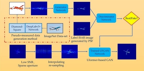
The overall imaging framework for maneuvering the target is shown in Figure 2. By setting different motion parameters for the simulated scattering points, ISAR echoes with motion errors can be obtained. As analyzed in Section 2, the resulting ISAR images by the RD algorithm are blurred in azimuth direction due to the phase error introduced by the target maneuver. The generator is to transform the blurred image into the deblurred image, and the discriminator is to determine and distinguish whether the generated image is real or fake. The generator and the discriminator fight each other until the discriminator can barely distinguish between real and fake images.

Some ISAR images obtained from measured data have small sizes and low resolution due to the small number of range samples or azimuth samples. Existing data-driven DL imaging methods generally directly input the small-size and low-resolution images to neural networks, and the restoration effect is limited by the small number of pixel points of the images. The network cannot learn enough features to recover the details and textures of the images and, therefore, cannot obtain high-quality ISAR images.

In this paper, we add a “resize” operation in the training stage and testing stage to increase the size of small images by performing BiCubic interpolation before they are input to the network. Moreover, delicate label images with higher resolution and finer details are also presented. Ideal ISAR images are obtained by convolving the coordinates of simulated scattered points with PSF, so it is easy to obtain delicate label images by the simulated training data. This operation has two benefits. Firstly, it helps the network to learn more hidden layer features and obtain high-quality ISAR images. Secondly, the image is resized before it is input to the network so that the network can keep the input and output images with the same resolution, thus avoiding the need to adjust the network parameters and retrain when the input and output images are of different sizes.

In the testing stage, due to the publicly available measured echo data of maneuvering targets being rare, we used the ISAR-measured echo data of smooth targets to equivalently generate the echoes of maneuvering targets by means of the Fourier interpolation method. The details of the method are given in Section 4.

3.2. Design of the Proposed UFGAN

In our design of UFGAN, the adversarial mode of GAN is adopted to make the deblurred images generated by the network closer to the ideal high-quality ISAR images. The locally-enhanced window (LeWin) Transformer blocks and the learnable multi-scale restoration modulators are used to build a novel generator to restore more image details. Global GAN and PatchGAN are combined to construct a new Transformer-based discriminator to improve the discrimination criteria of generated images by comprehensively evaluating global information and texture features. The Charbonnier loss, perceptual loss, and adversarial loss are combined to construct a comprehensive loss function to match the design of the network.

3.2.1. Generator

The overall architecture of the proposed generator is a symmetric hierarchical structure following the spirits of U-Net, as shown in Figure 3. The generator consists of an encoder, a bottleneck, a decoder, and several multi-scale restoration modulators. The input is the blurred ISAR image represented by ${\mathit{I}}_b\in {\mathit{R}}^{H\times W\times 3}$, with the image size of $H\times W$ and the channels of 3. Firstly, a 3 × 3 convolution with LeakyReLU is adopted to extract the shallow features represented by ${\mathit{X}}_0\in {\mathit{R}}^{H\times W\times C}$. Then ${\mathit{X}}_0$ is fed into four consecutive encoder levels. Each level includes several LeWin Transformer blocks connected in series and a down-sampling operation of a 4 × 4 convolution with stride two. After each level, the height and width of the feature maps are halved while the feature channels are doubled. Next, LeWin Transformer blocks connected in series as the bottleneck layer are used to capture longer dependencies.

The decoder has a symmetric structure with the encoder. Similarly, each decoder level consists of an up-sampling operation of 2 × 2 transposed convolution with stride two and a group of LeWin Transform blocks. Each level doubles the height and width of the feature maps while halving the feature channels. Owing to the design of the skip connection, the feature maps fed into the next decoder level are the concatenation of the output of the up-sampling layer and the features from the corresponding encoder level.

The multi-scale restoration modulators are denoted as learnable tensors with the shape of $M\times M\times C$, where M indicates the size of the window. The modulators are attached to all non-overlapping windows separately and act as a shared bias to calibrate features, which improves the adaptability of the network and promotes recovering more detail.

At last, the feature maps output from the encoder are flattened to two-dimensional feature maps and sent to the output projection layer with a 3 × 3 convolution. Then the residual image ${\mathit{I}}_r\in {\mathit{R}}^{H\times W\times 3}$ is produced and superimposed on the input image to generate a deblurred high-resolution ISAR image ${\mathit{I}}_0={\mathit{I}}_b+{\mathit{I}}_r({\mathit{I}}_0\in {\mathit{R}}^{H\times W\times 3})$.

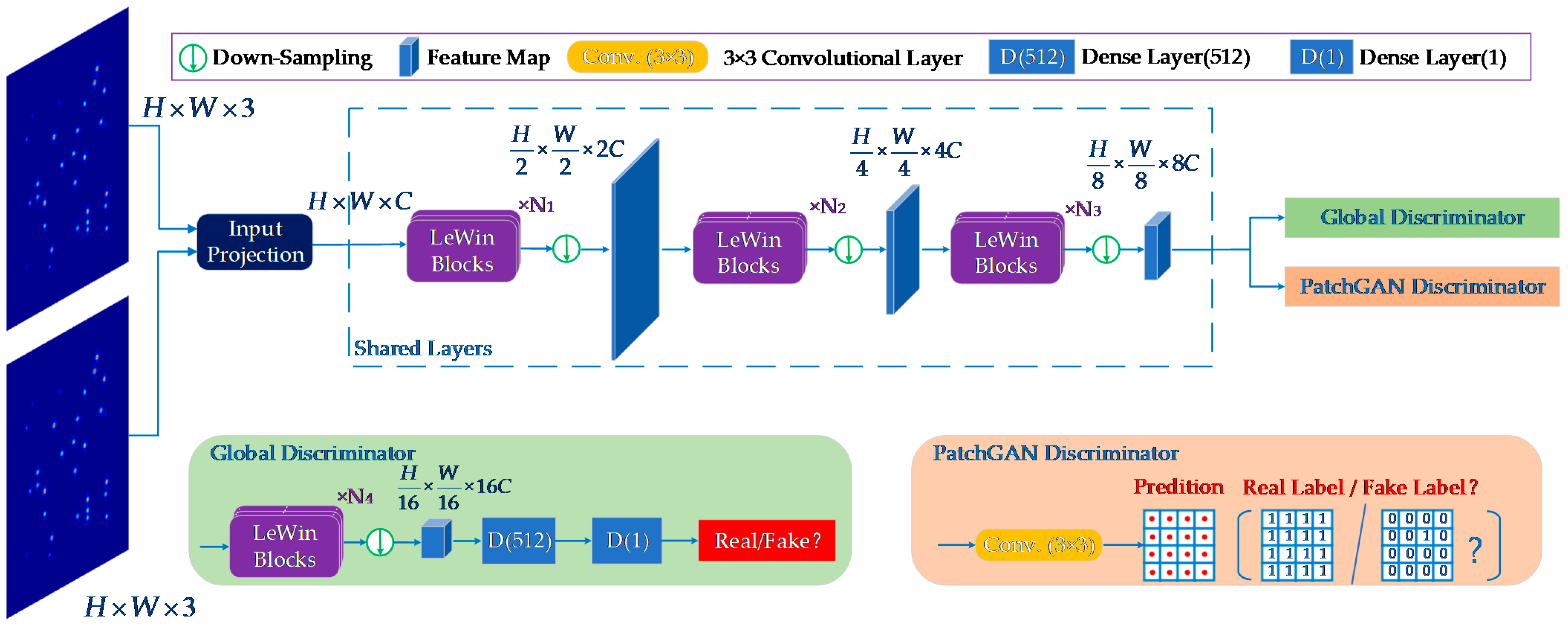
3.2.2. Discriminator

Traditional global discriminator aims to distinguish between the generated and real images by considering images holistically without focusing on whether the patches are well-matched to the global image. In contrast, PatchGAN [32] slides a window over the input image and obtains a scoring matrix to judge whether each patch is real or fake, which is more effective in revealing local details and capturing high-resolution.

In the design of our proposed discriminator, as shown in Figure 4, global GAN and PatchGAN are fused. Firstly, a shared layer consisting of LeWin Transform blocks and down-sampling layers is presented to extract shallow features, which have a similar structure to the encoder in the generator. After three levels, the network is divided into two paths. In one path, two dense layers are used, with channels 512 and 1 following an encoding layer to extract the global features. The other path employs a 3 × 3 convolutional layer to output a feature matrix containing all patch-level features for evaluating the local texture details.

By incorporating the two paths of global GAN and PatchGAN, the overall architecture integrates the local context and global information and provides a comprehensive evaluation of the image as a whole, as well as the consistency in local details.

The performance of the generator and discriminator is constantly improved as they work against each other, and the network eventually outputs deblurred images close to the real ISAR images.

3.2.3. LeWin Transformer Block

Standard Transformer structure has two disadvantages in image restoration. Firstly, it exploits the global self-attention on feature maps, leading to high computational costs as quadratic to the size of the feature maps. Secondly, the Transformer suffers a limited capability of leveraging local context, which is significant to restore deblurred ISAR images with high resolution.

Unlike the standard Transformer, the LeWin Transformer block performs a multi-head self-attention (W-MSA) for the non-overlapping local windows to reduce the computational cost, as shown in Figure 5. Moreover, the traditional Feed-Forward network is improved by adding a deep convolutional layer to enhance its local expression ability as the Locally-enhanced Feed-Forward Network (LeFF).

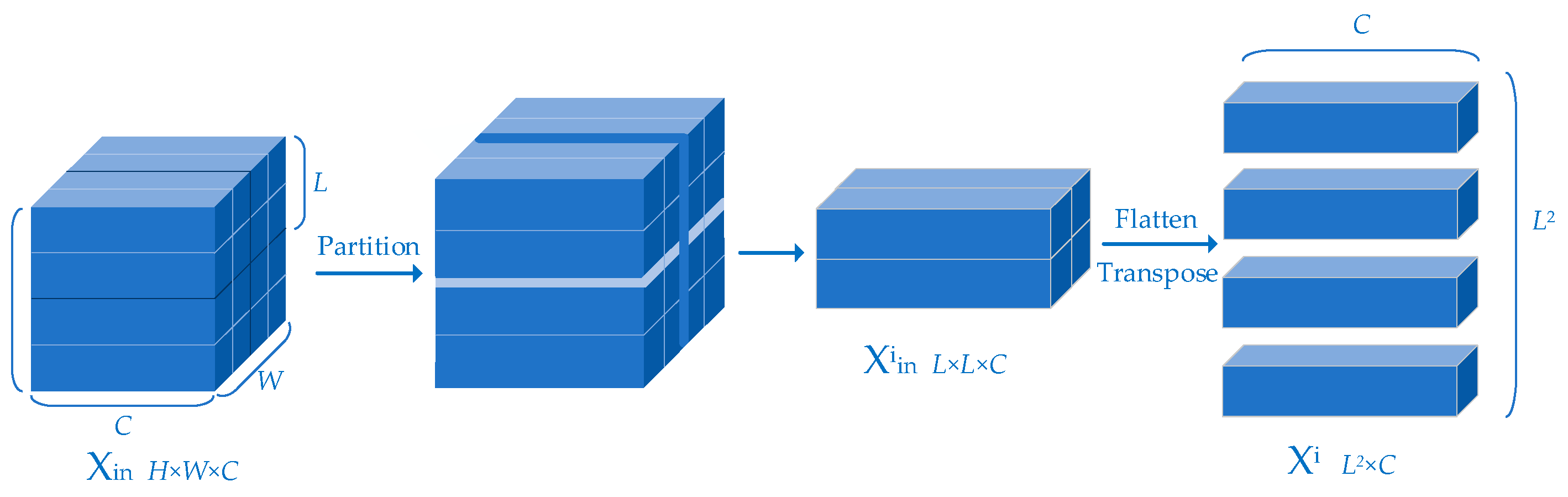
Figure 6 illustrates how the feature map is divided into non-overlapping windows.

Suppose the feature map ${\mathit{X}}_{\mathrm{input}}\in {\mathit{R}}^{H\times W\times C}$ is partitioned into non-overlapping windows of the size of $M\times M$, the feature map in the i-th window ${\mathit{X}}_{\mathrm{input}}^i\in {\mathit{R}}^{L\times L\times C}$ is flattened and transposed to be as ${\mathit{X}}^i\in {\mathit{R}}^{M^2\times C}$, where $i\in \left\{1,2,\dots ,N\right\}$, $N=HW/M^2$. Next, by applying self-attention, ${\mathit{X}}^i$ is projected to the query, key and value represented by ${\mathit{Q}}^i,{\mathit{K}}^i$ and ${\mathit{V}}^i\in {\mathit{R}}^{L^2\times C}$, respectively:

$${\mathit{Q}}^i={\mathit{X}}^i{\mathit{W}}^Q,{\mathit{K}}^i={\mathit{X}}^i{\mathit{W}}^K,{\mathit{V}}^i={\mathit{X}}^i{\mathit{W}}^V$$

(16)

where ${\mathit{W}}^Q$, ${\mathit{W}}^K$ and ${\mathit{W}}^V$ are the projection matrices. Next, ${\mathit{Q}}^i$, ${\mathit{K}}^i$ and ${\mathit{V}}^i$ are respectively divided into k heads:

$${\mathit{Q}}^i=\left\{{\mathit{Q}}_1^i,\dots ,{\mathit{Q}}_k^i\right\},{\mathit{K}}^i=\left\{{\mathit{K}}_1^i,\dots ,{\mathit{K}}_k^i\right\},{\mathit{V}}^i=\left\{{\mathit{V}}_1^i,\dots ,{\mathit{V}}_k^i\right\}$$

(17)

The Self-Attention (SA) for the j-th head can be written as:

$$\mathit{SA}\left({\mathit{Q}}_j^i,{\mathit{K}}_j^i,{\mathit{V}}_j^i\right)=\mathrm{softmax}\left(\frac{{\mathit{Q}}_j^i{\mathit{K}}_j^i{}^T}{\sqrt{C/k}}\right){\mathit{V}}_j^i$$

(18)

The output feature map ${\mathit{X}}_{\mathrm{output}}^i\in {\mathit{R}}^{L\times L\times C}$ of the i-th window can be obtained by concatenating the above attention value and being reshaped:

$${\mathit{X}}_{\mathrm{output}}^i=\mathrm{Reshape}(\underset{j=1}{\overset{k}{\mathrm{Concat}}}(SA({\mathit{Q}}_j^i,{\mathit{K}}_j^i,{\mathit{V}}_j^i)){\mathit{W}}^O+\mathit{P})$$

(19)

where $\mathrm{Reshape}(\cdot )$ presents the reshaping operation and $\mathrm{Concat}(\cdot )$ presents concatenating, ${\mathit{W}}^O\in {\mathit{R}}^{C\times C}$ denotes learnable parameters, and $\mathit{P}\in {\mathit{R}}^{M^2\times C}$ denotes the embedding position information. At last, the output feature maps of all image patches $\left\{{\mathit{X}}_{\mathrm{output}}^1,{\mathit{X}}_{\mathrm{output}}^2,\dots ,{\mathit{X}}_{\mathrm{output}}^N\right\}$ are combined to obtain the overall feature map of the entire image ${\mathit{X}}_{\mathrm{output}}\in {\mathit{R}}^{H\times W\times C}$.

Adjacent pixels are the essential references for image restoration, but the present Feed-Forward Network (FFN) in the standard Transformer shows a limitation in extracting local context information. The design of LeFF overcomes this drawback by adding a 3 × 3 depth-wise convolutional layer to the Feed-Forward Network.

The design of the LeWin Transformer Block can obviously reduce the computational cost. Given the feature map ${\mathit{X}}_{\mathrm{input}}\in {\mathit{R}}^{H\times W\times C}$, the computational complexity of the standard Transformer is $O\left(H^2{W}^{2}C\right)$, while the computational complexity of the LeWin Transformer module is $O\left(\frac{HW}{M^2}{M}^{4}C\right)=O\left(M^{2}HWC\right)$.

3.3. Loss Function

The role of the loss function is to optimize the network in the expected direction during training. Different designs of the loss function will improve the performance of the output images in different aspects. Using a combination of several kinds of loss functions can improve the overall performance of the output images.

3.3.1. The Charbonnier Loss

Exploiting Mean Square Error (MSE) as the loss function promotes a high peak signal-to-noise ratio (PSNR) of the reconstruction results. However, the high-frequency information is easily lost, and the over-smooth texture will appear by MSE, which will make some weak scatterers disappear in ISAR images. In order to overcome this issue, the Charbonnier loss function is adopted as follows:

$$L_{\mathit{char}}({\mathit{I}}_o,\mathit{I})=\sqrt{{\Vert {\mathit{I}}_o-\mathit{I}\Vert }^2+{\epsilon }^2}$$

(20)

where ${\mathit{I}}_o$ is the output deblurred ISAR image, $\mathit{I}$ is the ideal unblurred ISAR image, and $\epsilon =10^{-3}$ [31,36,37] is a constant to stabilize the value in experiments.

3.3.2. The Perceptual Loss

In order to achieve high-quality ISAR imaging while removing the blur, the perceptual loss focusing on image texture and edge features is used. Instead of calculating the loss between the output image and the ideal image directly, the key idea of perceptual loss is to compare the feature maps of the real image and the generated image, enhancing the similarity in feature space. The perceptual loss can be formulated by:

$$L_{perc}({\mathit{I}}_o,\mathit{I})=\frac{1}{H_i{W}_i{C}_i}{\Vert {\mathit{X}}_{\mathit{output}}^i-\phi \left({\mathit{I}}_H\right)\Vert }_2^2$$

(21)

where $H_i$, $W_i$,$C_i$ represent the height, width and channel of the feature map, ${\mathit{X}}_{\mathit{output}}^i$ represents the output feature map of the i-th layer and $\phi (\cdot )$ is a function to obtain the feature map of an image. We select the fourth layer to calculate the perceptual loss.

3.3.3. The Adversarial Loss

The classic generative adversarial loss of GAN suffers from training difficulties, unstable gradients and mode collapse, etc. In order to train the network stably, the adversarial loss function of Wasserstein GAN with gradient penalty (WGAN-GP) proposed by Ishaan et al. is used [38]. WGAN-GP presents the definition of the Earth-Mover (EM) distance, and the objective function can be derived as:

$$\underset{G}{\min } \underset{D}{\max }\mathit{V}\left(\mathit{G},\mathit{D}\right)=-{\mathit{E}}_{{\mathit{I}}_O~\mathit{P}\left({\mathit{I}}_O\right)}\left[\mathit{D}\left(\mathit{G}\left({\mathit{I}}_O\right)\right)\right]+{\mathit{E}}_{\mathit{I}~\mathit{P}\left(\mathit{I}\right)}\left[\mathit{D}\left(\mathit{I}\right)\right]-\lambda {\mathit{E}}_{{\mathit{I}}_{\mathit{Pena}}~\mathit{P}\left({\mathit{I}}_{\mathit{Pena}}\right)}\left[{\left({\Vert \mathbf{\nabla }\mathit{D}\left({\mathit{I}}_{\mathit{Pena}}\right)\Vert }_2-1\right)}^2\right]$$

(22)

where E represents taking average value, ${\mathit{I}}_{\mathit{Pena}}$ represents the sample image imposed a penalty. $P(\cdot )$ indicates the distribution of the image, $G(\cdot )$ and $D(\cdot )$ indicate the output of the generator and discriminator, respectively. $\mathbf{\nabla }$ indicates the gradient, $\lambda$ is the gradient penalty coefficient and the last term is the additional gradient penalty to constrain network training. The discriminator loss and generator loss with gradient penalty can be written as:

$${\mathit{L}}_{\mathit{adv}}^D={\mathit{E}}_{{\mathit{I}}_O~\mathit{P}\left({\mathit{I}}_O\right)}\left[\mathit{D}\left(\mathit{G}\left({\mathit{I}}_O\right)\right)\right]-{\mathit{E}}_{\mathit{I}~\mathit{P}\left(\mathit{I}\right)}\left[\mathit{D}\left(\mathit{I}\right)\right]+\lambda {\mathit{E}}_{{\mathit{I}}_{\mathit{Pena}}~\mathit{P}\left({\mathit{I}}_{\mathit{Pena}}\right)}\left[{\left({\Vert \mathbf{\nabla }\mathit{D}\left({\mathit{I}}_{\mathit{Pena}}\right)\Vert }_2-1\right)}^2\right]$$

(23)

$$L_{adv}^{\mathit{G}}=-{\mathit{E}}_{{\mathit{I}}_O~\mathit{P}\left({\mathit{I}}_O\right)}\left[\mathit{D}\left(\mathit{G}\left({\mathit{I}}_O\right)\right)\right]$$

(24)

3.3.4. The Overall Loss Function

Finally, the overall loss function can be obtained by the weighted sum of the above three loss functions:

$$\mathit{L}={\mathit{L}}_{\mathit{char}}({\mathit{I}}_o,\mathit{I})+{\lambda }_1{L}_{perc}({\mathit{I}}_o,\mathit{I})+{\lambda }_2\left({\mathit{L}}_{G\text{-}adv}^D+L_{G\text{-}adv}^G\right)+{\lambda }_3\left({\mathit{L}}_{P\text{-}adv}^D+L_{P\text{-}adv}^G\right)$$

(25)

where ${\lambda }_1$, ${\lambda }_2$, ${\lambda }_3$ are three tradeoff parameters to control the balance of the combination of loss functions. In specific, the generator parameters are updated by overall loss $\mathit{L}$, the global GAN path and the PatchGAN path are trained by ${\lambda }_2\left({\mathit{L}}_{G\text{-}adv}^D+L_{G\text{-}adv}^G\right)$ and ${\lambda }_3\left({\mathit{L}}_{P\text{-}adv}^D+L_{P\text{-}adv}^G\right)$, respectively. The generator and discriminator are trained in steps. During each mini-batch, firstly, the discriminator is fixed when training the generator, and then the generator is fixed when training the discriminator.

4. Data Generation

4.1. Generation of Simulated Targets

In practice, the scattering points on a target do not always emerge individually but exist in the form of regions or blocks. According to the scattering distribution characteristics behaved in ISAR images, we divide the imaging targets into two categories, i.e., point targets and block targets. Point targets are composed of individual scattering points and can be easily simulated by setting up randomly distributed scattering points. However, for a block target, the spectrum of the ISAR image is mixed and superimposed due to the aggregation characteristics of the scattering points, leading to rich image details and texture information. The block targets simulated by simple shapes are quite different from the real data.

Existing data-driven DL methods directly use the network trained by simulated point targets to image the measured block targets. However, this approach only preserves the pixels with large magnitudes as the individual scattering points, ignoring the weak scatters around and losing a lot of image details. In this paper, we propose a pseudo-measured data generation method to generate a variety of block targets with similar scattering distributions of the real measured data. Due to our focus on imaging for aircraft targets, the generation of various pseudo-measured aircraft block targets is taken as an example, as shown in Figure 7.

The processing steps of the method can be presented as follows:

The first step is to acquire varieties of aircraft geometric outlines. We use the images under “aeroplane” category in the PASCAL VOC2012 Augmented Dataset [39] to train the DeepLabv3+ network to be able to specifically segment geometric outlines from images containing aircraft targets. Next, by inputting images under the categories of “airliner” and “warplane” in the ImageNet2012 dataset [40] at a total of 2602 into the trained network model, 2602 images of aircraft geometric outlines are finally obtained.

The second step is gridding. Each aircraft geometric outline is meshed and mapped to a plane Cartesian coordinate with the size of 40 m × 40 m.

The third step is to generate random blocks within the gridded aircraft geometric outlines. The Diamond-Square algorithm is a random terrain generation algorithm that can randomly generate terrains with various shapes, such as mountains, hills, and oceans, in the grid of virtual scenes. Inspired by this, we refer to the Diamond-Square algorithm to randomly generate continuous scattering blocks within the aircraft’s geometric outlines.

Starting from the initial conditions, the scattering coefficient grid is continuously refined and calculated through the Diamond step and the Square step. The Diamond step is to calculate the scattering coefficient of the intersection of the square diagonals by a 2D random midpoint displacement algorithm, and the Square step is to calculate the scattering coefficients of the midpoint of each side of the square with the same random offset as the Diamond step. The detailed algorithm steps can be found in Appendix A.

Through the iterative calculation of the two steps, the scattering coefficients of all grid points can be obtained. Some examples of the generated block targets are shown in Figure 8.

4.2. Acquisition of Blurred ISAR Images

For simulated targets, the blurred ISAR images of maneuvering targets can be easily obtained according to Equation (15). However, for real data, most of the publicly available ISAR-measured data are collected from the detection of stationary moving targets. To address the problem that the measured ISAR data of real maneuvering targets are scarce, the Fourier interpolating re-sampling method is used to generate the equivalent ISAR echo data of maneuvering targets based on the existing measured data of smooth targets.

As indicated in Section 2, for a maneuvering target, the uniform motion or uniform acceleration motion model is not enough to accurately describe the motion state of the target. By retaining the third derivative term of displacement with respect to time, the motion state of the target is modeled as a variable acceleration motion as:

$$\omega ={\omega }_0+\beta t+\frac{1}{2}\gamma t^2$$

(26)

where ${\omega }_0$, $\beta$, $k$ represent the angular velocity, the angular acceleration and the angular jerk of the target, respectively.

Assuming that the slow time sampling interval is $T_l$ and the number of azimuth sampling is $N_l$ when the target rotates at a uniform angular velocity ${\omega }_l$, and the total angle the target rotates during the CPI can be calculated by:

$$\Omega ={\omega }_l\left(N_l-1\right)T_l$$

(27)

When the target rotates the same angle $\Omega$ with variable acceleration as shown in Equation (26), assuming that the angular velocity increment caused by angular acceleration is $P{\omega }_0$, the angular acceleration increment caused by the angular jerk $\gamma$ is $Q\beta$, the radar slow time sampling interval is $T\prime$, and the number of sampling is $N\prime$, we can obtain:

$$\{\begin{array}{c}{\omega }_l\left(N-1\right)T_l={\omega }_0\left(N\prime -1\right)T\prime +\frac{1}{2}\beta {\left[\left(N\prime -1\right)T\prime \right]}^2+\frac{1}{6}\gamma {\left[\left(N\prime -1\right)T\prime \right]}^3\\ P{\omega }_0=\beta \left(N\prime -1\right)T\prime +\frac{1}{2}\gamma {\left[\left(N\prime -1\right)T\prime \right]}^2\\ Q\beta =\gamma \left(N\prime -1\right)T\prime \end{array}$$

(28)

The above system of equations can be solved as:

$$\{\begin{array}{l}T\prime =\frac{N_l-1}{\left(N\prime -1\right)\left(\frac{3+Q}{3Q+6}P+1\right){\omega }_0}\\ \beta =\frac{\left(\frac{3+Q}{3Q+6}P+1\right)P{\omega }_0{}^2}{\left(N_l-1\right)\left(0.5Q+1\right)}\\ \gamma =\frac{{\left(\frac{3+Q}{3Q+6}P+1\right)}^2\mathrm{PQ}{\omega }_0{}^3}{{\left(N_l-1\right)}^2\left(0.5Q+1\right)}\end{array}$$

(29)

When observing the variable acceleration moving target, the rotation angle at the n-th $\left(n\in \left[0,N-1\right]\right)$ sample point can be calculated as

$$\begin{array}{cc}\hfill {\Omega }_n^{\prime }& ={\omega }_0{T}^{\prime }n+\frac{1}{2}\beta {\left(n{T}^{\prime }\right)}^2+\frac{1}{6}\gamma {\left(n{T}^{\prime }\right)}^3\hfill \\ \hfill & =\frac{N_l-1}{N^{\prime }-1}\xi (P,Q)n+\frac{\left(N_l-1\right)P}{{\left(N^{\prime }-1\right)}^2(Q+2)}\xi (P,Q)n^2+\frac{\left(N_l-1\right)PQ}{{\left(N^{\prime }-1\right)}^3(3Q+6)}\xi (P,Q)n^3\hfill \end{array}$$

(30)

where $\xi (P,Q)=\frac{3+Q}{3Q+6}P+1$.

Since the radar pulse repetition interval is fixed, the uniformly moving target is sampled with an equal interval, while the variable-speed moving target is sampled with an unequal interval. Therefore, the slow-time sampling signal of the variable-acceleration moving target can be obtained by performing interpolating re-sampling on the echo of the uniform moving target according to the displacement change rule indicated by Equation (30).

Suppose the slow time sampling signal of the uniform moving target is $s\left({\Omega }_n\right)$, by converting the distance axis of the signal into the time axis, the slow time sampling sequence $s\left(n\right)$ can be obtained. The discrete Fourier transform of $s\left(n\right)$ is:

$$X\left(k\right)={\displaystyle \sum _{n=0}^{N-1}s\left(n\right)}\cdot \exp (-j2k\pi \frac{n}{N}),k\in \left[-\left(N-1\right)/2,\left(N-1\right)/2\right]$$

(31)

Assuming that the slow time sampling signal of the variable acceleration moving target is $s\left({\Omega }_n^{\prime }\right)$, the interpolated slow time sampling sequence of the variable acceleration moving target $s\prime \left(n\right)$ can be obtained by inverse Fourier transform as:

$$\begin{array}{cc}\hfill s^{\prime }\left(n\right)& =s\left({\Omega }_n^{\prime }\right)\hfill \\ & =s\left(\left(N_l-1\right)\xi (P,Q)\left[\frac{n}{N\prime -1}+\frac{P{n}^2}{{\left(N\prime -1\right)}^2\left(Q+2\right)}+\frac{\mathrm{PQ}{n}^3}{{\left(N\prime -1\right)}^3\left(3Q+6\right)}\right]\right)\hfill \\ & =\frac{1}{N_l}{\displaystyle \sum _{k=-\left(N_l-1\right)/2}^{k=\left(N_l-1\right)/2}S\left(k\right)}\cdot \exp \left\{\mathrm{j}\frac{2\pi }{N_l}\xi (P,Q)\left(N_l-1\right)\left[\frac{n}{N\prime -1}+\frac{P{n}^2}{{\left(N\prime -1\right)}^2\left(Q+2\right)}+\frac{\mathrm{PQ}{n}^3}{{\left(N\prime -1\right)}^3\left(3Q+6\right)}\right]\right\}, n\in \left[0,N\prime -1\right]\hfill \end{array}$$

(32)

According to Equation (32), once we know the velocity increment P and acceleration increment Q of the variable acceleration movement during the CPI period, we can perform interpolating re-sampling through the slow time sampling sequence of uniform motion with the same moving distance and obtain the equivalent slow time sampling sequence of the maneuvering target.

4.3. Acquisition of Label ISAR Images

As shown in Figure 1, assuming the total rotation angle during CPI is Ω, the echo signal of the target can be regarded as the sum of the backscattered field of each scattering point as:

$$E^S\left(k,\Omega \right)={\displaystyle \sum _{i=1}^N{\sigma }_i\cdot \exp \left[-\mathrm{j}2\left(k\mathit{cos}\Omega \cdot x_i+k\mathit{sin}\Omega \cdot y_i\right)\right]}$$

(33)

where $N$ represents the total number of scattering points on the target, ${\sigma }_i$ is the scattering coefficient, and $\left(x_i,y_i\right)$ is the coordinate location for the i-th scattering point. $k$ represents the wave number. Under the condition of small angle, $k$ can be approximated as $k\approx k_c=2\pi f_c/c$, where $f_c$ is the center frequency and $k_c$ is the wave number. Therefore, Equation (33) can be simplified as:

$$E^S\left(k,\Omega \right)={\displaystyle \sum _{i=1}^N{A}_i\cdot \exp \left(-\mathrm{j}\frac{2\pi f_c}{c}{x}_i\right)}\cdot \exp \left(-\mathrm{j}\frac{2\pi \Omega }{\lambda }{y}_i\right)$$

(34)

For ISAR imaging, the two-dimensional point spread response (PSR) of range direction and azimuth direction can be expressed by:

$$h\left(x,y\right)=\left[\frac{2B}{c}\sin c\left(\frac{2B}{c}x\right)\exp \left(j\frac{4\pi f_c}{c}x\right)\right]\cdot \left[\frac{2\Omega }{\lambda }\sin c\left(\frac{2\Omega }{\lambda }y\right)\exp \left(j\frac{4\pi {\Omega }_c}{\lambda }y\right)\right]$$

(35)

where B represents the bandwidth of the transmitting signal. ${\Omega }_c$ represents the central value of the coherent accumulation angles.

The ideal ISAR imaging of all scattering points on a target can be obtained by 2D inverse Fourier integral (2D-IFFT) of the echo signal $E^S\left(k,\Omega \right)$ as:

$$\begin{array}{cc}\hfill ISAR(x,y)& =\sum _{i=1}^N\underset{k_{min}}{\overset{k_{max}}{\int }}\underset{{\Omega }_{min}}{\overset{{\Omega }_{max}}{\int }}{E}^S(k,\Omega )·exp\left[\mathrm{j}2\left(kcos\Omega ·x_i+ksin\Omega ·y_i\right)\right]d\left(\frac{2f}{c}\right)·d\left(\frac{k_c\Omega }{\pi }\right)\hfill \\ \hfill & =\sum _{i=1}^N{A}_i·\delta \left(x-x_i,y-y_i\right)\ast h(x,y)\hfill \end{array}$$

(36)

where $k_{\min }$ and $k_{\max }$ represent the minimum and maximum values lower of the spatial frequency. ${\Omega }_{\min }$ and ${\Omega }_{\max }$ represent the initial and final look-angles, $\delta \left(x,y\right)$ is the impulse response.

It can be seen from Equation (36) that the 2D ISAR imaging result is nothing but the convolution of the position coordinates of all scattering points on the target with the 2D PSF function.

5. Experiments

In this section, we conduct simulation and measured experiments on ISAR imaging for maneuvering point targets and block targets based on the proposed UFGAN. The imaging results and imaging times are compared with the classical RD algorithm, which is for smooth targets, and STFT, WVD, SPWVD, and RWT algorithms which are used for maneuvering targets. The image entropy (IE), structural similarity (SSIM), target-to-clutter ratio (TCR), and imaging time are used as evaluation metrics to quantitatively evaluate the performance of different methods.

5.1. ISAR Imaging for Maneuvering Point Targets

The publicly available Boeing-727 data from V.C. Chen [41] are typical echo data of a point target. The numbers of range cells and azimuth cells are 64 and 256, respectively. The radar transmits a signal with a bandwidth of 150 MHz and a PRF of 20 KHz. The carrier frequency is 9 GHz. In order to ensure the best performance of the proposed method on Boeing-727 data, the same radar parameters are set for all simulated scattering point targets. The training set consists of 500 point targets, which are composed of randomly distributed scatter points.

As analyzed in Section 2, the blurring level of the image depends on the parameters $K_{\beta \omega }$ and $K_{\gamma \beta }$. Considering the achievability of the maneuver, in reality, we first restrict the value of $K_{\beta \omega }$ and $K_{\gamma \beta }$ to be randomly taken between 0 to 5. Then the initial angular velocity ${\omega }_0$ is set to be randomly taken in the range of 0.01~0.1 rad/s. The angular acceleration $\beta$ and the jerk $\gamma$ can be naturally determined by the above three parameters. In other words, ${\omega }_0$, $K_{\beta \omega }$ and $K_{\gamma \beta }$ completely determined the motion state of the target. In order to improve the imaging performance of the network under sparse aperture and low SNR, the echo is added with the additive white Gaussian noise (AWGN) of SNR = −10 dB~10 dB and down-sampled at the sampling ratio of 20−80% in the azimuth direction. In this paper, the sampling ratio indicates the ratio of the number of retained samples after down-sampling to the total number of samples. The training stage went through 250 epochs and cost 3 h in total.

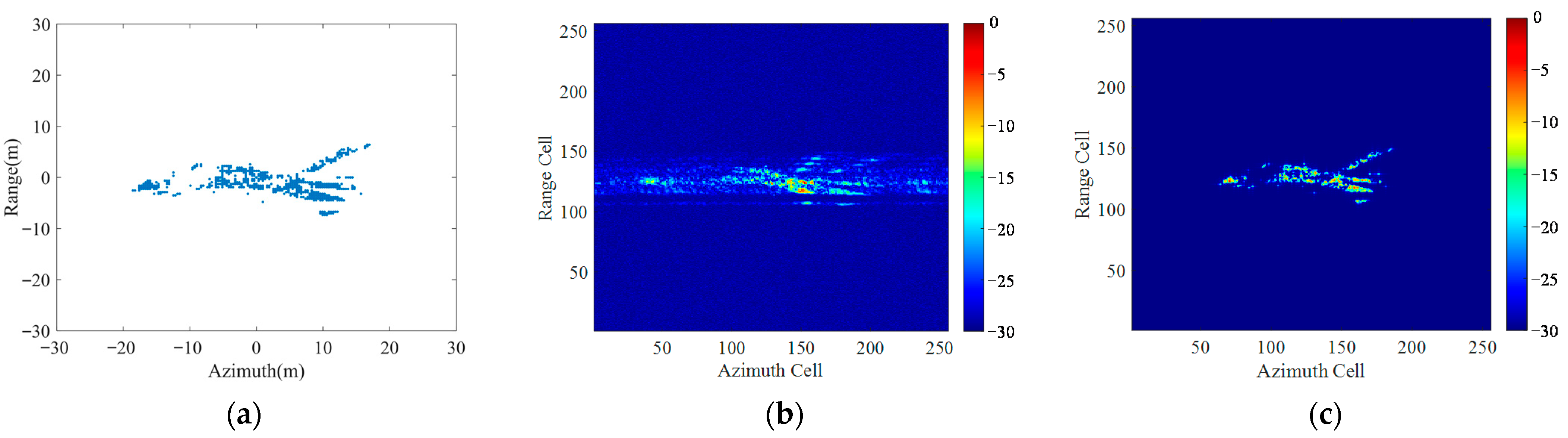
Figure 9 shows a training sample. Figure 9a presents the coordinate distribution of the scattering points on the point target. The motion parameters are: ${\omega }_0=0.024$ rad/s, $K_{\beta \omega }=3.5$, $K_{\gamma \beta }=4.5$, thus the angular acceleration and the jerk can be calculated as $\beta =\omega K_{\beta \omega }=0.084$ rad/s², $\gamma =\beta K_{\gamma \beta }=0.378$ m/s³. Figure 9b presents the blurred imaging result by the RD method under a 30% sampling ratio with SNR = 0 dB. The ideal ISAR image without any phase error is generated according to Equation (36), as shown in Figure 9c.

5.1.1. Simulated Experiments

A simulated aircraft model of 74 points, as shown in Figure 10, is used to test the trained UFGAN network.

Assuming that the motion compensation has been completed, the target equivalently rotates at a variable acceleration. We set different motion parameters and conducted three experiments with different noise levels and sampling ratios. The motion parameters and imaging conditions are presented in

Table 1. The motion parameters and imaging conditions of the three experiments.

Parameters and Conditions	Experiment 1	Experiment 2	Experiment 3
angular velocity(rad/s)	0.08	0.06	0.03
angular acceleration(rad/s2)	0.16	0.12	0.12
angular jerk(rad/s3)	0.16	0.48	0.48
relative acceleration ratio	2	2	4
relative jerk ratio	1	4	4
SNR	∞	−3 dB	−7 dB
sampling rate	100%	70%	30%

.

The imaging results of the three experiments are presented in Figure 11. We can see that the high-resolution deblurred ISAR images can always be recovered with different motion parameters and signal conditions.

According to Table 1 and Figure 11, several conclusions that concluded from Equation (15) can be verified: (i) The degree of blurring of the ISAR image for a maneuvering target obtained by RD algorithm does not depend on the magnitude of its angular velocity, angular acceleration or angular jerk, but on their proportional relationship, i.e., the value of relative acceleration ratio $K_{\beta \omega }$ and relative jerk ratio $K_{\gamma \beta }$. (ii) The blurring of the target is gradually serious as $K_{\beta \omega }$ and $K_{\gamma \beta }$ increase. In the case of short imaging time, $K_{\gamma \beta }$ has less effect on the degree of image blurring than $K_{\beta \omega }$.

5.1.2. Imaging Experiments of Public BOEING-727 Data

Boeing-727 data from Victor C. Chen are used to verify the effectiveness of the proposed method on real ISAR data. In order to demonstrate the superiority of the proposed method, we select several traditional methods for comparison.

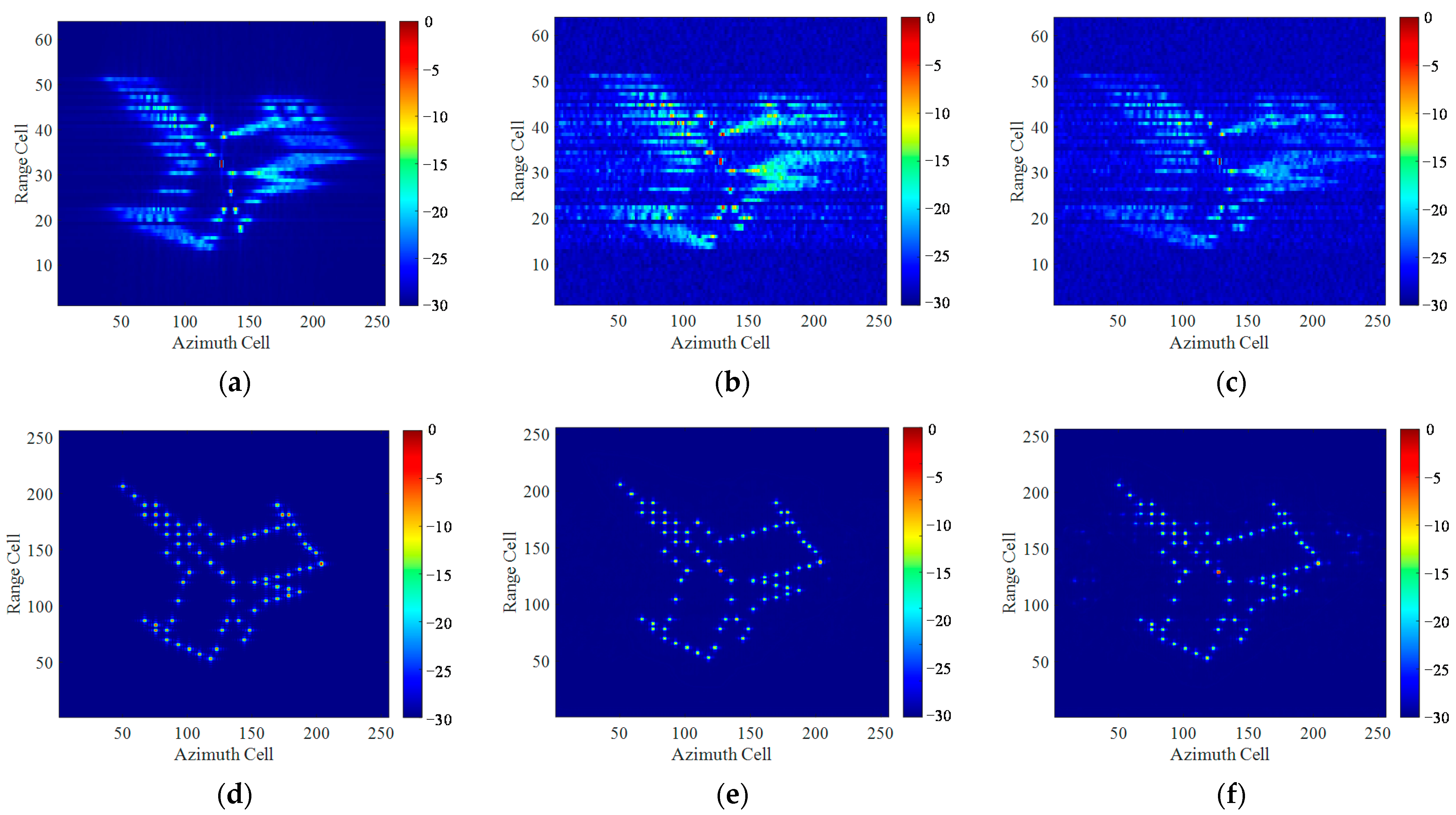
Figure 12 presents the imaging results of different methods under full aperture without adding any noise. It can be seen that the imaging result by RD method is heavily blurred in the azimuth direction. STFT method has eliminated the main blurring of the image but suffers a low time-frequency resolution. ISAR images by WVD method have a better resolution, but cross-terms appear, degrading the quality of the imaging result. SPWVD method succeeds in suppressing the cross-terms but reduces the frequency resolution and loses some weak scattering points. RWT method effectively improves the azimuth focusing of the image, but there still exists some blurring and smearing. Compared with the above traditional methods, the proposed method achieves high-resolution restoration of the ISAR images without any blurring.

The second experiment is to verify the imaging performance of the proposed method under low SRN conditions by adding noise to the Boeing-727 echo. Figure 13 presents the imaging results under SNR = −10 dB by different methods. It can be seen that the ISAR images obtained by traditional methods are seriously degraded, that the target can be barely distinguishable due to the interference of the noise. By contrast, Figure 13f shows that the UFGAN network can effectively restore the blurred image even in a scenario with strong noise. Although there exist several hot pixels in the background, the target subject is still reconstructed with high quality.

Table 2. The evaluation indicators of different methods under SNR = −10 dB.

Method	IE	TCR/dB	Imaging Time/s
RD	5.7428	40.1519	0.0172
STFT	5.5962	48.6892	2.9459
WVD	4.3157	57.6743	10.2687
SPWVD	4.5298	46.4851	41.9245
RWT	3.4477	64.5826	16.7458
Proposed method	0.8452	87.7593	0.1903

gives the values of the evaluation indicators of the traditional algorithms and the proposed method for Figure 13. For the Boeing-727 data, we cannot obtain the label ISAR image, so the SSIM could not be used as evaluation indicator in this experiment. The RD algorithm is far superior to other traditional algorithms in imaging time, but the image quality is the worst according to the value of IE and TCR. The proposed method outperforms other traditional algorithms a lot in imaging quality and imaging time.

The third experiment is to verify the imaging performance of the proposed method under sparse aperture. Figure 14a gives the down-sampled echo signal with a sampling ratio of 40%. Figure 14b–f presents the imaging results under sparse aperture by different methods. It can be seen that the target is subject to different degrees of spectral occlusion by traditional algorithms. By contrast, a high-resolution image with clear background is obtained by the proposed method.

Table 3. The evaluation indicators of different methods under sparse aperture.

Method	IE	TCR/dB	Imaging Time/s
RD	4.7843	43.4688	0.0154
STFT	4.8854	51.0240	2.6851
SPWVD	3.3482	57.9647	38.4186
RWT	1.5861	72.4875	15.2943
Proposed method	0.7585	85.4582	0.1884

gives the values of the evaluation indicators by the traditional algorithms and the proposed method for Figure 14. It can be seen that the proposed method achieves superior performance compared with the traditional method, and the imaging is shorter than traditional methods except RD algorithm.

5.2. ISAR Imaging for Maneuvering Block Targets

In this section, we use the pseudo-measured dataset presented in Section 4 to carry out imaging experiments for maneuvering block targets. The radar parameters are set as the same as measured Yak-42 data, where the size of the echo matrix is 256 × 256, the carrier frequency is 5.52 GHz, the bandwidth is 400 MHz, the pulse width is 25.6 µs, and the PRF is 400 Hz.

The motion parameters of the training data are set as the same as the training point targets in Section 5.1. Then the blurred ISAR images and ideal label ISAR images are generated according to Equation (15) and Equation (36), respectively, which together form the paired pseudo-measured ISAR image sets.

In order to enhance the robustness of the network, sparse aperture and low SNR are considered. The noise of SNR randomly distributed in the range of −10 dB~10 dB is added to the pseudo-measured echoes, and the sampling ratio is randomly distributed in the range of 20–80%. We allocate 80% of the paired images as the training set and the remaining 20% as the test set to train the UFGAN network. The training stage went through 300 epochs and cost 7 h in total.

Figure 15 gives a sample of the training set. Figure 15a presents the coordinate distribution of the scattering points on the block target. The motion parameters of the block target are: ${\omega }_0=0.072$ rad/s, $K_{\beta \omega }=4.0$, $K_{\gamma \beta }=1.5$, thus the angular acceleration and the jerk can be calculated as $\beta =\omega K_{\beta \omega }=0.288$ rad/s² and $\gamma =\beta K_{\gamma \beta }=0.432$ m/s³. Figure 15b presents the blurred ISAR imaging result by RD method under 35% sampling ratio with the noise level of SNR = 0 dB. Figure 15c presents the ideal imaging result.

5.2.1. Simulated Experiments

We chose a block target from the test set to test the effectiveness of the trained UFGAN network. The coordinate distribution and ideal ISAR image of the block target are shown in Figure 16.

We conducted four experiments with different motion parameters and imaging conditions, as presented in

Table 4. The motion parameters and imaging conditions of the four experiments.

Parameters and Conditions	Exp.1	Exp.2	Exp.3	Exp.4
angular velocity (rad/s)	0.02	0.04	0.06	0.08
angular acceleration (rad/s2)	0.08	0.04	0.12	0.24
angular jerk (rad/s3)	0.08	0.16	0.36	0.48
relative acceleration ratio	4	1	2	3
relative jerk ratio	1	4	3	2
SNR	∞	0 dB	−8 dB	−12 dB
sampling ratio	100%	45%	25%	15%

.

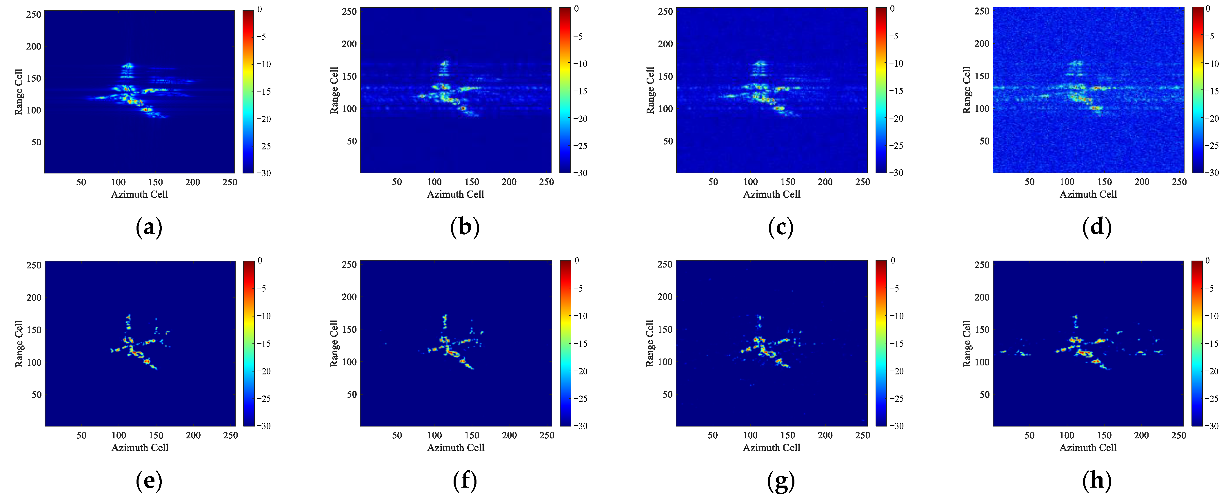
Figure 17 shows the imaging results of the four experiments. It can be seen that under the condition of acceptable noise level and sampling ratio, the blurred ISAR images of the maneuvering block targets can be effectively restored by the network to high-quality images without phase error. Even under more extreme imaging conditions, as shown in Figure 17d,h, the target subject region of the image can still be deblurred though there appear some hot pixels.

5.2.2. Measured Experiments

In the data acquisition process of Yak-42 aircraft by ISAR experimental radar, the movement with little maneuver can nearly be considered as a uniform motion during CPI. The Yak-42 echo can be imaged by RD algorithm to receive the unblurring ISAR image as shown in Figure 18.

To verify the performance of the trained UFGAN in maneuvering block target imaging, we adopt the Fourier interpolation re-sampling method as given in Section 4 to generate the echo data of the maneuvering target on the basis of the original Yak-42 data. The motion parameters are set as: the angular velocity of 0.03 rad/s, angular acceleration of 0.1 rad/s², and angular jerk of 0.4 rad/s³. Several time-frequency analysis methods and parameter estimation methods are also presented to be compared with the proposed method. For the reason that cross-term issues of the WVD method have particularly serious impact on block targets, leading to a poor imaging result, it is no longer used as a comparison algorithm in the Yak-42 imaging experiment.

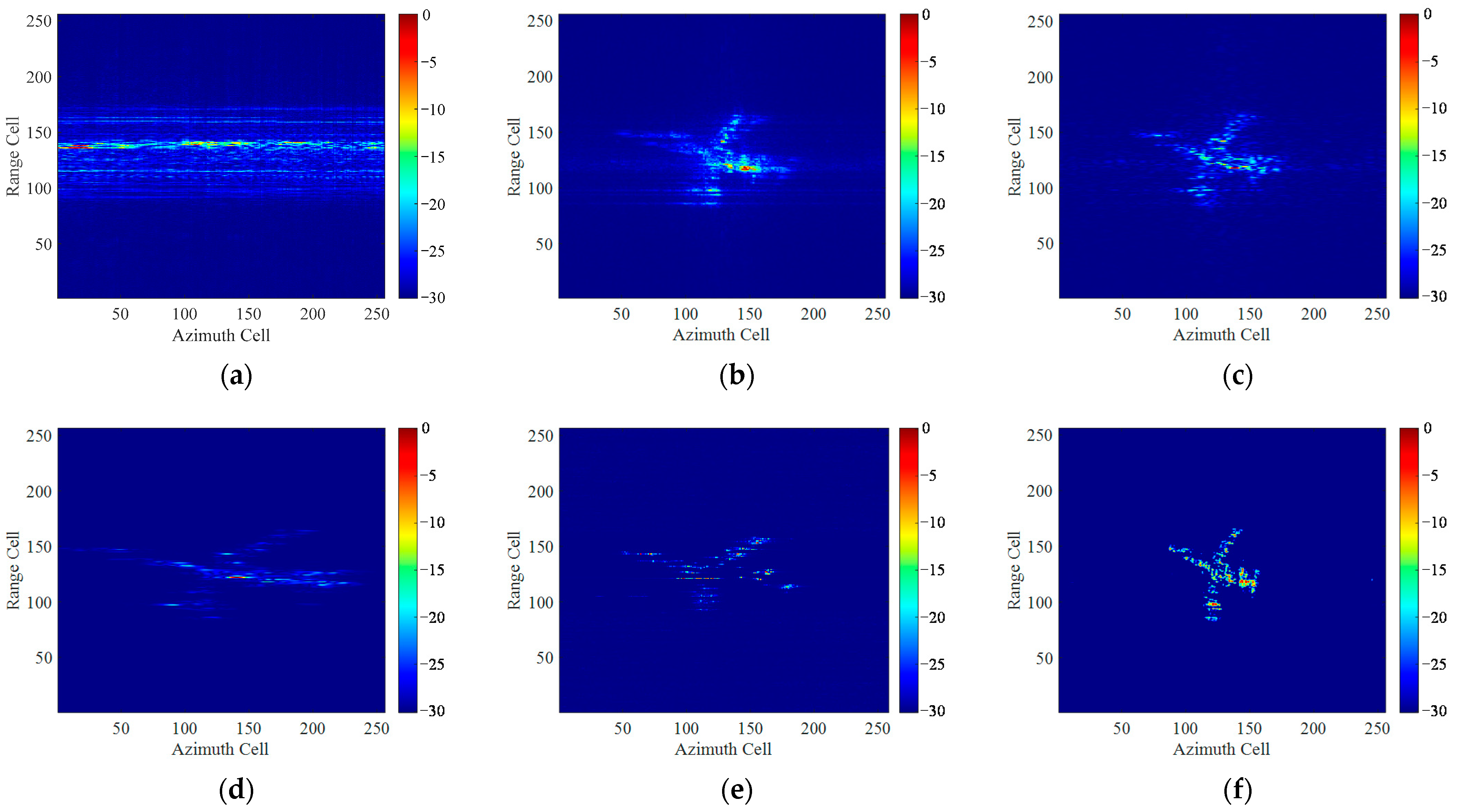
Figure 19 shows the imaging results without adding extra noise under full aperture. Figure 19a presents the “dechirped” echo after motion compensation. Figure 19b–f presents the imaging results by several traditional algorithms. It can be seen that the spectrum is heavily expanded along azimuth direction by RD algorithm. STFT algorithm alleviates the blurring issue of the image but has a low time-frequency resolution. The SPWVD method suppresses the cross-terms at the expense of stretching the spectrum in the azimuth direction, and the image contrast is severely decreased. RWT method improves the time-frequency resolution but has a weak ability to distinguish weak scattering areas from background noise, leading to a structural loss of the target scatterers. By contrast, the proposed method achieves superior performance, reconstructing a high-resolution ISAR image with rich details and fine textures.

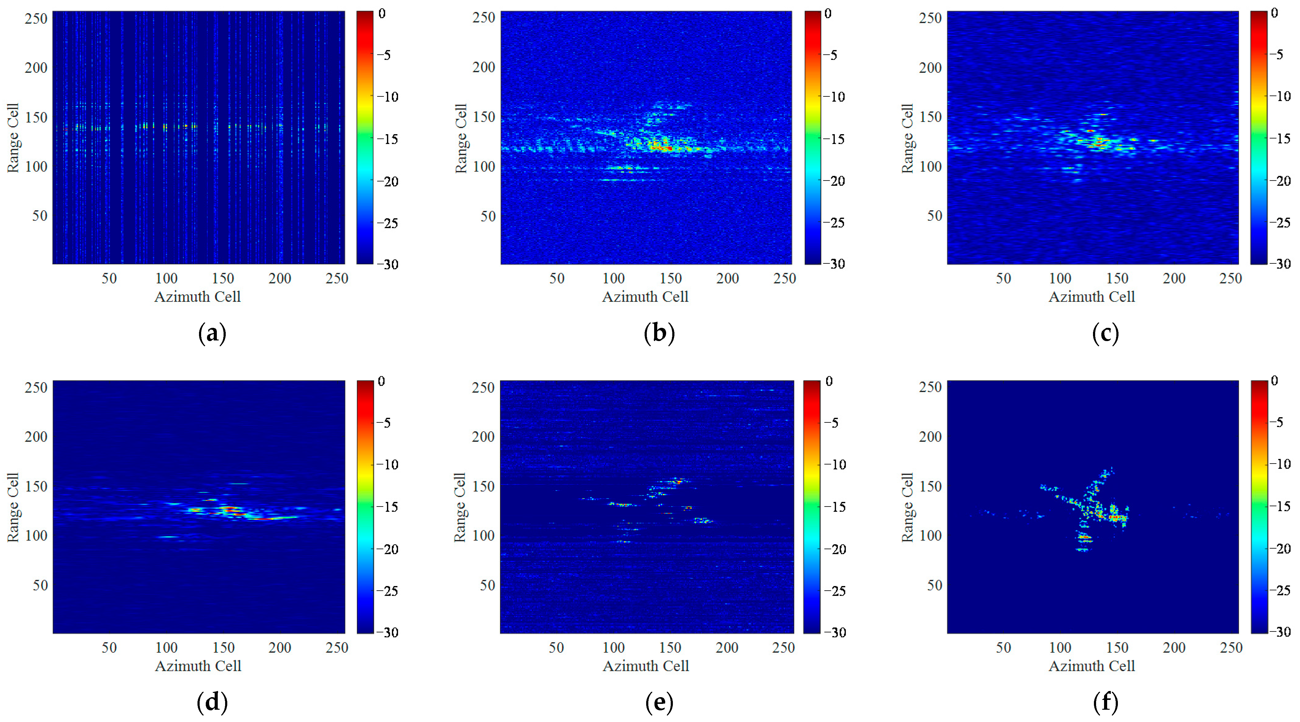
Figure 20 and Figure 21 present the imaging results under the condition of different noise levels and sparse aperture. Figure 20a and Figure 21a present the down-sampled echo at the sampling ratio of 50% and 25% with SNR = 0 dB and −10 dB, respectively. Figure 20b–f and Figure 21b–f present the imaging results of different methods. The motion parameters are set as: the angular velocity of 0.05 rad/s and 0.08rad/s, angular acceleration of 0.2 rad/s² and 0.24 rad/s², and the angular jerk of 0.8 rad/s³ and 0.72 rad/s³, respectively. It can be seen that due to the presence of noise and sparse aperture, the quality of ISAR images obtained by traditional methods declined sharply. Especially under the condition of strong noise and low sampling ratio, as shown in Figure 20, the target has been nearly completely submerged in noise and spectral occlusion, to be hardly distinguished from the degraded images. However, the deblurred high-resolution ISAR image with rich details and fine textures can still be restored by UFGAN network, though several hot pixel blocks appear in the background.

Table 5. The evaluation indicators of different methods under sparse aperture.

Experiment	Method	IE	SSIM	TCR/dB	Imaging Time/s
Exp.1: 50% sampling ratio, SNR = 0 dB	RD	4.8816	0.1256	56.8569	0.014
	STFT	4.6124	0.1921	61.5164	2.8795
	RWT	4.1125	0.0845	55.5218	16.2416
	SPWVD	3.3162	0.0917	67.5682	38.1458
	Proposed method	2.4356	0.8163	91.2041	0.195
Exp.2: 25% sampling ratio, SNR = −10 dB	RD	6.0847	0.0933	41.2958	0.0015
	STFT	5.8726	0.1284	44.5291	2.8851
	RWT	4.5482	0.0684	47.5126	16.2541
	SPWVD	3.7159	0.0761	58.1259	37.1567
	Proposed method	2.5214	0.8047	89.4582	0.186

gives the evaluation indicators of the imaging results of the above two experiments by traditional algorithms and the proposed method for Figure 20 and Figure 21. Due to the Yak-42 data being collected from smooth target, the imaging result of the original echo by RD algorithm is unblurred, which can be used as the ideal image to calculate the SSIM. It can be seen that under the condition of sparse aperture and low SNR, the imaging performance of traditional methods seriously deteriorated, while the proposed method achieves fast and high-quality reconstruction of the ISAR images.

5.3. Performance Comparison with Existing Data-Driven Methods

To demonstrate that the proposed UFGAN-based method shows better performance in restoring the details and texture features of ISAR images compared with the existing data-driven methods, we selected an ISAR super-resolution imaging method based on improved GAN recently proposed by Wang H et al. [22]. It is a typical data-driven method, and, like most data-driven methods, it uses randomly distributed scattering points as the training set. We conducted an imaging comparison experiment on the measured Yak-42 data. Figure 22 presents the imaging results of the measured Yak-42 data. The first, second, and third lines give the imaging results under ideal imaging conditions, SNR = 0 dB at 50% sampling ratio and SNR = −10 dB at 25% sampling ratio, respectively. It can be seen that the imaging result by RD algorithm is seriously blurred along azimuth direction. The imaging result by method in [22] achieves super-resolution, but the ISAR images lose a lot of fine structural information, as shown in Figure 22b,e,h, and the outline of the target in the obtained ISAR image are stretched along the azimuth, and the shape of the target is distorted due to the maneuverability of the target. In contrast, the proposed method can achieve unblurring ISAR imaging with more details and fine textures, reconstructing the geometric shape and structure of the target more accurately.

To verify the robustness of the proposed UFGAN, Figure 23 presents the performance curves of more comparison results of the proposed DL-based methods with the traditional methods and method in [22] under the condition of different SNR and different sampling ratios. The motion parameters of Yak-42 data are kept unchanged, which is the same as the experiment presented in Figure 19. In order to control variate, the sampling ratio is fixed to be 50% in Figure 23a, and the SNR is fixed to be 0 dB in Figure 23b. It can be seen that imaging results by the proposed method have the minimum IE under various SNR and sampling rate conditions compared with the traditional methods.

It is worth noting that although some evaluation indicators, e.g., the IE, of the method in [22] are smaller than that of the proposed method under various SNR and sampling rate conditions, it loses many weak scattering points in the ISAR image and could hardly restore the details and texture features of the image as shown in Figure 22, leading to the distortion of the ISAR images in detail, while the proposed method performs better in unblurring reconstruction of high-quality ISAR images, retaining more detail and texture features.

6. Conclusions

For ISAR imaging of maneuvering targets, the existing deep learning methods could not avoid the blurring of ISAR images without the assistance of traditional methods such as RID and show a weak ability to restore image details and textures. In this article, a novel unblurring ISAR imaging method for maneuvering targets based on UFGAN is proposed. Firstly, according to the derivation of the azimuth echo signal with the form of a QFM signal, the blurred ISAR images for network training are obtained. To improve the generalization in measured data, we propose a pseudo-measured data generation method based on the DeepLabv3+ network and the Diamond-Square algorithm. Then we use the LeWin blocks and multi-scale restoration modulators to build a novel UFGAN, which can effectively restore the image details. The discriminator is designed by combining the PatchGAN and global GAN to aggregate the local and global information to provide a comprehensive evaluation of the image as a whole as well as the consistency in local details. A comprehensive loss function to consider both perceptual loss and adversarial loss is designed to match the performance of the network. In the test stage, to verify the effectiveness of the network on the measured data, Fourier interpolating re-sampling is used to obtain the equivalent ISAR echo of maneuvering targets. Finally, we conducted simulated and measured experiments and comparisons under sparse aperture and low SNR conditions to verify the effectiveness and efficiency of the proposed method.

Noticing that the proposed method cannot succeed in effectively imaging multiple maneuvering targets because the motion parameters of each target are different. In order to cope with the issue, a recognition module might be needed to distinguish different objects in one imaging scene according to the degree of blurring, and then different partitions of the image can be processed separately.

References

- Chen, V.C.; Martorella, M. Inverse Synthetic Aperture Radar Imaging: Principles, Algorithms and Applications; SciTech Publishing: Edison, NJ, USA, 2014; pp. 116–123. [Google Scholar]
- Chen, V.C.; Qian, S. Joint time-frequency transform for radar range Doppler imaging. IEEE Trans. Aerosp. Electron. Syst. 1998, 34, 486–499. [Google Scholar] [CrossRef]
- Fu, J.; Xing, M.; Sun, G. Time-Frequency Reversion-Based Spectrum Analysis Method and its Applications in Radar Imaging. Remote Sens. 2021, 13, 600. [Google Scholar] [CrossRef]
- Wang, Y.; Huang, X.; Zhang, Q.X. Rotation parameters estimation and cross-range scaling research for range instantaneous Doppler ISAR images. IEEE Sens. J. 2020, 20, 7010–7020. [Google Scholar] [CrossRef]
- Chen, V.C.; Miceli, W.J. Time-varying spectral analysis for radar imaging of maneuvering targets. IET Proc. Radar Sonar Navig. 1998, 145, 262–268. [Google Scholar] [CrossRef]
- Xing, M.D.; Wu, R.B.; Li, Y.C.; Bao, Z. New ISAR imaging algorithm based on modified Wigner Ville distribution. IET Proc. Radar Sonar Navig. 2009, 3, 70–80. [Google Scholar] [CrossRef]
- Lv, Y.; Wang, Y.; Wu, Y.; Wang, H.; Qiu, L.; Zhao, H.; Sun, Y. A Novel Inverse Synthetic Aperture Radar Imaging Method for Maneuvering Targets Based on Modified Chirp Fourier Transform. Appl. Sci. 2018, 8, 2443. [Google Scholar] [CrossRef] [Green Version]
- Li, J.; Ling, H. Application of adaptive chirplet representation for ISAR feature extraction from targets with rotating parts. IEEE Proc. Radar Sonar Navig. 2003, 150, 284–291. [Google Scholar] [CrossRef]
- Li, W.C.; Wang, X.S.; Wang, G.Y. Scaled radon-Wigner transform imaging and scaling of maneuvering target. IEEE Trans. Aerosp. Electron. Syst. 2010, 46, 2043–2051. [Google Scholar] [CrossRef]
- Yiğit, E.; Demirci, Ş.; Özdemir, C. Clutter removal in millimeter wave GB-SAR images using OTSU’s thresholding method. Int. J. Eng. Sci. 2022, 7, 43–48. [Google Scholar] [CrossRef]
- Duysak, H.; Yiğit, E. Investigation of the performance of different wavelet-based fusions of SAR and optical images using Sentinel-1 and Sentinel-2 datasets. Int. J. Eng. Sci. 2022, 7, 81–90. [Google Scholar] [CrossRef]
- Bayramoğlu, Z.; Uzar, M. Performance analysis of rule-based classification and deep learning method for automatic road extraction. Int. J. Eng. Sci. 2023, 8, 83–97. [Google Scholar] [CrossRef]
- Zhao, S.Y.; Zhang, Z.H.; Zhang, T.; Guo, W.W.; Luo, Y. Transferable SAR Image Classification Crossing Different Satellites under Open Set Condition. IEEE Geosci. Remote Sens. Lett. 2022, 19, 1–5. [Google Scholar] [CrossRef]
- Kang, L.; Sun, T.C.; Luo, Y.; Ni, J.C.; Zhang, Q. SAR Imaging based on Deep Unfolded Network with Approximated Observation. IEEE Geosci. Remote Sens. 2022, 60, 1–14. [Google Scholar] [CrossRef]
- Wei, S.; Liang, J.; Wang, M.; Zeng, X.; Shi, J.; Zhang, X. CIST: An Improved ISAR Imaging Method Using Convolution Neural Network. Remote Sens. 2020, 12, 2641. [Google Scholar] [CrossRef]
- Zhang, S.H.; Liu, Y.X.; Li, X. Computationally Efficient Sparse Aperture ISAR Autofocusing and Imaging Based on Fast ADMM. IEEE Trans. Geosci. Remote Sens. 2020, 58, 8751–8765. [Google Scholar] [CrossRef]
- Wei, S.J.; Liang, J.D.; Wang, M.; Shi, J.; Zhang, X.L.; Ran, J.H. AF-AMPNet: A Deep Learning Approach for Sparse Aperture ISAR Imaging and Autofocusing. IEEE Trans. Geosci. Remote Sens. 2022, 60, 5206514. [Google Scholar] [CrossRef]
- Liang, J.D.; Wei, S.J.; Wang, M.; Shi, J.; Zhang, X.L. Sparsity-driven ISAR imaging via hierarchical channel-mixed framework. IEEE Sens. J. 2021, 21, 19222–19235. [Google Scholar] [CrossRef]
- Wang, M.; Wei, S.; Liang, J.; Zeng, X.; Wang, C.; Shi, J.; Zhang, X. RMIST-Net: Joint Range Migration and Sparse Reconstruction Network for 3-D mmW Imaging. IEEE Trans. Geosci. Remote. Sens. 2021, 60, 1–17. [Google Scholar] [CrossRef]
- Hu, C.; Wang, L.; Li, Z.; Zhu, D. Inverse synthetic aperture radar imaging using a fully convolutional neural Network. IEEE Geosci. Remote Sens. Lett. 2020, 17, 1203–1207. [Google Scholar] [CrossRef]
- Yang, T.; Shi, H.Y.; Lang, M.Y.; Guo, J.W. ISAR imaging enhancement: Exploiting deep convolutional neural network for signal reconstruction. Int. J. Remote Sens. 2020, 41, 9447–9468. [Google Scholar] [CrossRef]
- Wang, H.; Li, K.; Lu, X.; Zhang, Q.; Luo, Y.; Kang, L. ISAR Resolution Enhancement Method Exploiting Generative Adversarial Network. Remote Sens. 2022, 14, 1291. [Google Scholar] [CrossRef]
- Yuan, Y.X.; Luo, Y.; Ni, J.C.; Zhang, Q. Inverse Synthetic Aperture Radar Imaging Using an Attention Generative Adversarial Network. Remote Sens. 2022, 14, 3509. [Google Scholar] [CrossRef]
- Luo, Y.; Ni, J.C.; Zhang, Q. Synthetic aperture radar learning-imaging method based on data-driven technique and artificial intelligence. J. Radars 2020, 9, 107–122. [Google Scholar]
- Shi, H.Y.; Lin, Y.; Guo, J.W.; Liu, M.X. ISAR autofocus imaging algorithm for maneuvering targets based on deep learning and keystone transform. J. Syst. Eng. Electron. 2020, 31, 1178–1185. [Google Scholar]
- Qian, J.; Huang, S.Y.; Wang, L.; Bi, G.A.; Yang, X.B. Super-resolution ISAR imaging for maneuvering target based on deep-learning-assisted time-frequency analysis. IEEE Trans. Geosci. Remote Sens. 2021, 60, 1–14. [Google Scholar] [CrossRef]
- Eldar, Y.C.; Kuppinger, P.; Bolcskei, H. Block-Sparse Signals: Uncertainty Relations and Efficient Recovery. IEEE Trans. Signal Process. 2010, 58, 3042–3054. [Google Scholar] [CrossRef] [Green Version]
- Gao, J.; Deng, B.; Qin, Y.; Wang, H.; Li, X. Enhanced radar imaging using a complex-valued convolutional neural network. IEEE Geosci. Remote Sens. Lett. 2019, 1, 35–39. [Google Scholar] [CrossRef] [Green Version]
- Chen, L.C.; Zhu, Y.; Papandreou, G.; Schroff, F.; Adam, H. Encoder-decoder with atrous separable convolution for semantic image segmentation. In Proceedings of the European Conference on Computer Vision (ECCV), Munich, Germany, 8–14 September 2018; pp. 801–818. [Google Scholar]
- Miller, G.S.P. The definition and rendering of terrain map. In Proceedings of the 13th Annual Conference on Computer Graphics and Interactive Techniques, New York, NY, USA, 9–13 August 1986; pp. 39–48. [Google Scholar]
- Wang, Z.D.; Cun, X.D.; Bao, J.M.; Zhou, W.G.; Liu, J.; Li, H. Uformer: A general u-shaped Transformer for image restoration. In Proceedings of the IEEE/CVF Conference on Computer Vision and Pattern Recognition (CVPR), New Orleans, LA, USA, 19–24 June 2022; pp. 17683–17693. [Google Scholar]
- Isola, P.; Zhu, J.Y.; Zhou, T.H.; Efros, A.A. Image-to-image translation with conditional adversarial networks. In Proceedings of the IEEE Conference on Computer Vision and Pattern Recognition (CVPR), Honolulu, HI, USA, 21–26 July 2017; pp. 1125–1134. [Google Scholar]
- Zhao, M.; Wang, M.; Chen, J.; Rahardja, S. Perceptual Loss-Constrained Adversarial Autoencoder Networks for Hyperspectral Unmixing. IEEE Geosci. Remote Sens. Lett. 2022, 19, 1–5. [Google Scholar] [CrossRef]
- Li, D.; Zhan, M.; Liu, H.; Liao, Y.; Liao, G. A robust translational motion compensation method for ISAR imaging based on keystone transform and fractional Fourier transform under low SNR environment. IEEE Trans. Aerosp. Electron. Syst. 2017, 53, 2140–2156. [Google Scholar] [CrossRef]
- Li, L.; Yan, L.; Li, D.; Liu, H.Q.; Zhang, C.X. A novel ISAR imaging method for maneuvering target based on AM-QFM model under low SNR environment. IEEE Access 2019, 7, 140499–140512. [Google Scholar] [CrossRef]
- Ahuja, N.; Lai, W.S.; Huang, J.B.; Yang, M.H. Deep Laplacian Pyramid Networks for Fast and Accurate Super-Resolution. In Proceedings of the 2017 IEEE/CVF Conference on Computer Vision and Pattern Recognition, Honolulu, HI, USA, 21–26 July 2017; pp. 5835–5843. [Google Scholar]
- Zamir, S.W.; Arora, A.; Khan, S.; Hayat, M.; Khan, F.S.; Yang, M.H.; Shao, L. Learning enriched features for real image restoration and enhancement. In Proceedings of the European Conference on Computer Vision (ECCV), Glasgow, UK, 23–28 August 2020; pp. 492–511. [Google Scholar]
- Gulrajani, I.; Ahmed, F.; Arjovsky, M.; Dumoulin, V.; Courville, A. Improved training of wasserstein GANs. In Proceedings of the 31st International Conference on Neural Information Processing Systems, Long Beach (NIPS), Long Beach, CA, USA, 3–9 December 2017; pp. 5769–5779. [Google Scholar]
- The PASCAL VOC2012 Augmented Dataset. Available online: http://host.robots.ox.ac.uk/pascal/VOC/voc2012/ (accessed on 11 August 2022).
- The ImageNet Dateset. Available online: https://image-net.org/ (accessed on 15 August 2022).
- Wang, Y.; Ling, H.; Chen, V.C. ISAR motion compensation via adaptive joint time–frequency technique. IEEE Trans. Aerosp. Electron. Syst. 1997, 34, 670–677. [Google Scholar] [CrossRef]
Figure 1.
The ISAR imaging geometry for maneuvering target.
Figure 2.
ISAR imaging framework for maneuvering target.
Figure 3.
The architecture of the proposed generator.
Figure 4.
The architecture of the proposed discriminator.
Figure 5.
Structure of LeWin Transformer blocks in series and the LeFF module.
Figure 6.
How the feature map is divided into non-overlapping windows.
Figure 7.
The generation process of pseudo-measured aircraft block targets.
Figure 8.
Some examples of the pseudo-measured block targets generation: (a) The origin images in dataset; (b) The segmented images; (c) The pseudo-measured targets.
Figure 9.
An example of the training data: (a) The coordinate distribution of the scattering points; (b) The blurred ISAR imaging result by RD method; (c) The ideal ISAR image.
Figure 10.
The simulated aircraft model: (a) The coordinate distribution of the scattering points; (b) The ideal ISAR image.
Figure 11.
Imaging results of simulated aircraft model with the motion parameters and imaging condition as listed in Table: (a–c) Imaging results by RD method; (d–f) Imaging results of the proposed method.
Figure 12.
Imaging results of Boeing-727 data under full aperture without noise by different methods: (a) RD algorithm; (b) STFT algorithm; (c) WVD algorithm; (d) SPWVD algorithm; (e) RWT algorithm; (f) the proposed method.
Figure 13.
Imaging results of Boeing-727 data with SNR = −10 dB by different methods: (a) RD algorithm; (b) STFT algorithm; (c) WVD algorithm; (d) SPWVD algorithm; (e) RWT algorithm; (f) the proposed method.
Figure 14.
Imaging results of Boeing-727 data under 40% sampling ratio by different methods: (a) The down-sampled echo signal; (b) RD algorithm; (c) STFT algorithm; (d) SPWVD algorithm; (e) RWT algorithm; (f) the proposed method.
Figure 15.
An example of the training data: (a) The coordinate distribution of the scattering points on the block target; (b) The blurred ISAR image as the input of UFGAN; (c) The ideal image as the label of the UFGAN.
Figure 16.
A block target sample from test set: (a) The coordinate distribution of the scattering points; (b) The ideal ISAR image.
Figure 17.
Imaging results of the block target with the motion parameters and imaging condition as listed in Table 2: (a–d) Imaging results by RD method; (e–h) Imaging results be the proposed method.
Figure 18.
The imaging result of the original echo by RD algorithm.
Figure 19.
Imaging results of Yak-42 measured data under full aperture without noise by different methods: (a) echo after translational motion compensation; (b) RD algorithm; (c) STFT algorithm; (d) SPWVD algorithm; (e) RWT algorithm; (f) The proposed method.
Figure 20.
Imaging results of Yak-42 under 50% sampling ratio with SNR = 0 dB by different methods: (a) echo after translational motion compensation; (b) RD algorithm; (c) STFT algorithm; (d) SPWVD algorithm; (e) RWT algorithm; (f) The proposed method.
Figure 21.
Imaging results of Yak-42 under 25% sampling ratio with SNR = −10 dB by different methods: (a) echo after translational motion compensation; (b) RD algorithm; (c) STFT algorithm; (d) SPWVD algorithm; (e) RWT algorithm; (f) The proposed method.
Figure 22.
Imaging results of Yak-42 by different methods: (a,d,g) RD algorithm; (b,e,h) The method in [22]; (c,f,i) The proposed method.
Figure 23.
Performance curves of IE versus SNR and sampling ratio of six different methods: (a) Performance curves of IE versus SNR; (b) Performance curves of IE versus sampling ratio.