
Assessment and Calibration of ERA5 Severe Winds in the Atlantic Ocean Using Satellite Data
by
 , , and
Ricardo M. Campos
1,2,* ,
,
Carolina B. Gramcianinov
3,4,
Ricardo de Camargo
4 and
Pedro L. da Silva Dias
4 1
Cooperative Institute for Marine and Atmospheric Studies (CIMAS), University of Miami, 4600 Rickenbacker Causeway, Miami, FL 33149, USA
2
NOAA Atlantic Oceanographic and Meteorological Laboratory (AOML), 4301 Rickenbacker Causeway, Miami, FL 33149, USA
3
Institute for Coastal Systems Analysis and Modeling, Helmholtz-Zentrum Hereon, Max-Planck-Straße 1, 21502 Geesthacht, Germany
4
Departamento de Ciências Atmosféricas, Instituto de Astronomia, Geofísica e Ciências Atmosféricas, Universidade de São Paulo, Rua do Matão 1226, Cidade Universitária, São Paulo 05508-000, Brazil
*
Author to whom correspondence should be addressed.
Remote Sens. 2022, 14(19), 4918; https://doi.org/10.3390/rs14194918
Submission received: 24 August 2022
/
Revised: 23 September 2022
/
Accepted: 28 September 2022
/
Published: 1 October 2022
(This article belongs to the Special Issue Remote Sensing of Wave Fields under Extreme Weather Conditions (in Tropical and Extra-Tropical Cyclones and Polar Lows))
Abstract
:In this paper, we analyze the surface winds of ECMWF ERA5 reanalysis in the Atlantic Ocean. The first part addresses a reanalysis validation, studying the spatial distribution of the errors and the performance as a function of the percentiles, with a further investigation under cyclonic conditions. The second part proposes and compares two calibration models, a simple least-squares linear regression (LR) and the quantile mapping method (QM). Our results indicate that ERA5 provides high-quality winds for non-extreme conditions, especially at the eastern boundaries, with bias between −0.5 and 0.3 m/s and RMSE below 1.5 m/s. The reanalysis errors are site-dependent, where large RMSE and severe underestimation are found in tropical latitudes and locations following the warm currents. The most extreme winds in tropical cyclones show the worst results, with RMSE above 5 m/s. Apart from these areas, the strong winds at extratropical locations are well represented. The bias-correction models have proven to be very efficient in removing systematic bias. The LR works well for low-to-mild wind intensities while the QM is better for the upper percentiles and winds above 15 m/s—an improvement of 10% in RMSE and 50% for the bias compared to the original reanalysis is reported.
1. Introduction
Marine winds have great importance in several ocean engineering sectors, including platform design and operations, oil spill modeling, ship routing, offshore wind energy, and alert of extreme events, among others. Besides these direct applications, surface winds on the ocean play a fundamental role in wave generation [1,2] and wave modeling [3,4,5,6], surface currents [7,8], and sea level changes [9,10]. Therefore, the accuracy of ocean winds gathers a wide range of direct and indirect elements supporting a variety of ocean modeling applications, including climate studies [11,12,13,14,15] and statistical analyses [16,17].
The lack of long-term metocean observations with broad spatial coverage in the open ocean has driven the development of global reanalyses, joining the state-of-the-art in numerical modeling with data assimilation of quality-controlled observations—especially remote sensing data. Since the 1990s, reanalyses have gained attention and importance in many scientific areas; the European Centre for Medium-Range Weather Forecasts (ECMWF) and the National Oceanic and Atmospheric Administration (NOAA) being the two main developers of publicly available global reanalyses. Several generations of reanalyses were produced by both centers, such as ERA40 [18], ERA-Interim [19], and ERA5 [20,21], produced by ECMWF, and the NCEP reanalysis 1 and 2 [22,23], followed by the NCEP climate forecast system reanalysis [24,25], produced by NOAA. Such products were extensively evaluated and discussed in the literature, e.g., Stopa and Cheung [25], Caires et al. [26], Campos and Guedes Soares [6,27], Sharp et al. [28], Zabolotskikh and Chapron [29], and Carvalho [30].
The most recent global reanalysis produced by ECMWF, which is widely used worldwide, is the Fifth European Centre for Medium-Range Weather Forecast Reanalysis (ERA5) [20,21,31]. The surface winds at 10 m height have a space–time resolution of 0.25° and 1 h, covering the period from 1979 to the present (recently expanded to 1950). Compared to ERA-Interim, ERA5 benefits from a decade of developments in model physics, core dynamics and data assimilation [32]. The ERA5 reanalysis is based on 4D-Var data assimilation using Cycle 41r2 of the Integrated Forecasting System (IFS) and the model has a significantly enhanced horizontal resolution of 31 km grid spacing compared to 79 km for ERA-Interim [19,32]. A key element that improves the quality of ERA5 is the great evolution of the observing system, where the number of observations assimilated has increased from approximately 0.75 million per day on average in 1979 to around 24 million per day by the end of 2018—satellite radiances being the dominant and growing type of data throughout the period [32].
ERA5 winds were deeply investigated [33,34,35], including validations using scatterometer data [36]. The aforementioned studies highlight the better quality of ERA5 compared to its predecessors. Molina et al. [34], for example, showed that comparisons with European stations exhibit hourly scores ranging from 0.8 to 0.9, indicating that ERA5 can reproduce the wind speed spectrum range. In the Black Sea, Çalışır et al. [35] confirmed the good performance of ERA5 but the authors reported an increasing underestimation of wind speeds of ERA5 and CFSR at high intensities—a common pattern discussed many times in the reanalysis products literature. They also show that ERA5 performs better than the CFSR in lower wind speeds and worse in higher wind speeds, while the overall assessment found ERA5 winds with less bias. Similarly, a comparison study by Gramcianinov et al. [37] found that CFSR presents stronger cyclones than ERA5. However, so far there is no study dedicated to marine winds evaluation covering the whole Atlantic Ocean while also including validation of the reanalysis at higher percentiles and under cyclonic conditions.
To address this demand, the present study performs a detailed assessment of ERA5 reanalysis winds (10 m height) in the Atlantic Ocean using satellite data, with special attention to the spatial distribution of the reanalysis errors. Furthermore, due to the large dataset of altimeters and scatterometers publicly available nowadays, our methodology subsamples the data to investigate the performance as a function of the percentiles and inside the cyclones in both hemispheres. This is a fundamental aspect to consider when selecting ERA5 to run extreme value analysis (EVA), which directly depends on the quality at the tail of the empirical distributions. Besides the assessment using maps of error metrics, our paper proposes a calibration model to help end-users of ERA5 to have more accurate data on wind speed in the Atlantic Ocean, allowing a link between the research and practical applications.
Our paper is organized as follows. Section 2 presents the initial comparisons and assessments, Section 3 has the calibration proposed to improve the accuracy of ERA5 winds, and Section 4 is focused on cyclonic conditions. Section 2, Section 3 and Section 4 are self-contained, describing the methodology and presenting the results. Section 5 summaries the discussion and analyses of four extreme events, including Hurricane Dennis (1999) and Hurricane Sandy (2012). The final Section 6 concludes the study.
2. Assessments
Since the priority of the present study is to discuss the spatial distribution of the reanalysis errors and to gather a large amount of data for the statistical analyses, the observations selected must go beyond traditional metocean buoys—restricted to single points usually close to the coast. Remote sensing plays a fundamental role in data assimilation in weather prediction systems [38] and consists of valuable information for model validation and calibration due to its global coverage—becoming a better source of data. Liu et al. [39], for example, successfully used scatterometer data to perform a characterization of tropical cyclone wind intensity. Ricciardulli and Manaster [40] reinforced that scatterometers provide very stable ocean wind data records, which was deeply investigated by Ribal and Young [41] and Young et al. [42]. Campos and Guedes Soares [6,27] provided validations of the reanalysis of winds and waves using altimeter data. A complete discussion about the accuracy of altimeter data can be found by Ribal and Young [43] and an additional assessment was performed by Yang et al. [44]. Fortunately, there are more than 20 years of high-quality satellite data of surface winds [42,45,46] publicly available.
In this context, our ERA5 validation and calibration in this study are performed using satellite data, joining altimeters and scatterometers, and leaving buoy data for the final event-based assessment of the calibrated results. The altimeter and scatterometer databases selected belong to the Australian Ocean Data Network (IMOS/AODN), which added great value to satellite data by applying quality control followed by calibration of each satellite mission. The dataset is also very organized and well documented, which facilitates its use. Ribal and Young [41,43,46] and Young et al. [42] described the data, including assessments and calibration. The following scatterometer missions were selected: ERS2, METOP-A, METOP-B, OCEANSAT-2, QUIKSCAT, and RAPIDSCAT—involving 430 G of data. The following altimeter missions were selected: TOPEX, ERS-2, GFO, JASON-1, ENVISAT, JASON-2, CRYOSAT-2, HY2, SARAL, JASON3, SENTINEL3-A, SENTINEL3-B—involving 110 G of data.
The validation and calibration in the next sections were firstly performed for each satellite mission aforementioned, independently, which led to hundreds of plots that compromise the interpretation of results. Initial findings showed that differences among satellites, including altimeters and scatterometers, are much smaller than the reanalysis errors. Besides the visual similarities of results, we quantitatively found general differences up to 0.7 m/s among satellite missions; however, such comparisons must be performed under certain criteria, such as the cross-validation matchup plots presented by Ribal and Young [43]. The authors indicated excellent agreement of wind speed among satellite missions, with most differences within the 0.5 m/s range. Therefore, it was decided to join the whole dataset in a unified analysis and discussion. Both validation and calibration were conducted in the domain shown in Figure 1, in the Atlantic Ocean from 62°S to 62°N, excluding polar latitudes to avoid the influence of ice.
2.1. Data Collocation and Error Metrics
The satellite tracks and swaths have very high resolution in space and time while ERA5 winds are restricted to 0.25° and 1 h. Therefore, a direct interpolation of reanalysis data to match the satellite data would input errors associated with spatio-temporal scales that are not simulated by the reanalysis—leading to misinterpretation of the real limitations of the reanalysis winds. Alternatively, the satellite data can be collocated to the ERA5 grid with hourly resolution. This involves a definition of maximum time and space for the selection of the satellite records, centered at the reanalysis grid points. At this point, understanding the typical spatio-temporal variation of surface winds is extremely important, in order to propose a suitable average of the satellite observations to compare with the reanalysis. The fundamental study of Monaldo [47] addressed this subject in depth by examining the differences between buoy and altimeter estimates as a function of space and time distances. This study gave support to the following papers and analyses using satellite collocation of wind speed and significant wave height, e.g., [28,48,49,50]. Following the methodology [48,49,50], the satellite records were collocated into the ERA5 grid using a maximum space distance of 25 km and a time distance of 0.5 h. The average was calculated using a Gaussian function that was applied to weight satellite records by distance to the grid point.
Next, a grid mask was built to analyze the water depth (ETOPO1) [51,52] and distance to the coast (GSFC/NASA, Figure 1A) of the grid points, taking the same latitude and longitude arrays from the ERA5 grid, selected for the Atlantic Ocean. Queffeulou and Croizé-Fillon [53], Young et al. [42], and Campos et al. [50] discussed the degraded accuracy of altimeters and scatterometers at coastal waters near land and they recommend excluding satellite data close to the coast. Therefore, a minimum water depth of 80 m and a distance to the nearest coast of 50 km were fixed at the grid mask to guarantee the satellite records are reliable and the matchups satellite/reanalysis can be used for validation and calibration (Figure 1B).
Considering the number of satellite missions and density of satellite data, as well as the accuracy of each satellite dataset [41,46] it was decided to restrict this study to a period starting in 2000. Thus, a total of 21 years, from 2000 to 2021, of ERA5 winds and AODN satellite data were selected. Figure 1C shows the total count of matchups satellite/reanalysis used throughout this study. Due to the polar orbit, the concentration is higher at polar latitudes. Smaller water bodies, such as lakes and seas, were excluded as well. Hence, only open water grid points in the Atlantic Ocean were selected.
The sequence of the next sections involves an initial comparison of datasets, followed by validation and calibration. The assessments are based on four error metrics presented by Equations (1)–(4), respectively: Bias, Root-Mean-Square-Error (RMSE), Scatter Index (SI), and Pearson’s correlation coefficient (CC). These are the same statistics selected by Ribal and Young [46], where is the reanalysis and are the observations. The overbar represents the arithmetic mean. The systematic component of the error is contained in the Bias (Equation (1)) while the scatter component is isolated in the SI (Equation (3)). A deeper explanation of these metrics and how to interpret them can be found in [54,55,56,57].
2.2. Initial Comparisons
The first comparisons between ERA5 wind speeds with satellite data are performed using the first three moments: mean, variance, and skewness. They reflect how well the distribution functions of both datasets agree with each other. For metocean analysis, especially extreme value analysis (EVA), the proper representation of the shape of the distribution is important to allow reliable extrapolations to longer return values—which depend on the variance and skewness. If the map shows positive skewness, the tail of the distribution tends to be longer and evolves towards higher values, i.e., the probability of strong winds is higher. Inversely, when the skew is negative and variance is low, the wind intensity rarely increases to values distant from the mean. Most importantly, the probabilistic moments are a simple way to use statistics to start investigating whether the physics implemented in the atmospheric model are properly representing the true environment state or not.
Figure 2 shows the direct comparison, with mean, variance, and skewness calculated for the exact same pairs of satellite/reanalysis in the 21 years selected. Figure 2A,D have very similar contours and patterns, indicating that ERA5 properly simulates the general atmospheric circulation regarding surface winds, with mean values varying from 4 m/s to 11 m/s. This result corroborates the global maps provided by Young et al. [42]. The westerlies and strong winds at mid-high latitudes are very similar between ERA5 and the satellites, both in terms of position and intensity. The Azores Anticyclone and the South Atlantic Anticyclone are also well positioned and well represented in ERA5. There are small differences between datasets, around 1 to 2.5 m/s, related to low winds at equatorial locations in the eastern portion of the Atlantic Ocean as well as in subtropical latitudes in the northwest part of the domain—where the satellite wind intensity is higher than ERA5. The variance and skewness panels confirm the quality of ERA5. The variance in the Northern Hemisphere is slightly higher (around 3 ) in satellite data than in ERA5, whereas for the South Atlantic both have more similar values—apart from the Malvinas Current, offshore Argentina, and the Benguela Current, offshore South Africa—which have small differences between datasets.
The skewness maps (Figure 2C,F) show higher positive values in the satellite data but the differences once again are very small, about 0.1 . Thus, the ERA5 winds provide an excellent representation of the first three probabilistic moments when compared to satellite data.
The next comparisons in Figure 3 show the percentiles, from 90 to 99, computed for each grid point and for both datasets (ERA5 and satellites), allowing a model evaluation as it progressively moves towards the tail of the distribution, in the most severe conditions. It is possible to see in Figure 3 the intensification of wind intensity at extratropical latitudes, mostly at locations with the largest positive skewness found in Figure 2F. The contours and patterns of ERA5 agree with the satellites once again. However, the differences in wind intensity at mid-high latitudes increase with the percentiles—pointing to lower winds of ERA5. The underestimation of ERA5 winds is more evident at the 95th and 99th percentiles when it reaches 8 to 10% of differences in the North Atlantic. Comparing the hemispheres, it is possible to see a better agreement in the Southern Hemisphere while the ERA5 underestimation north of 35°N becomes more evident. This feature has a significant impact on the statistical analysis of extreme winds and waves in the North Atlantic Ocean.
It is interesting to observe that the progressive underestimation of ERA5 winds in the North Atlantic responds to the higher wind intensification of the mid-high latitudes compared to the tropical part—which is also coherent with the higher skewness values of Figure 2F in the North Atlantic. The limitations of ERA5 winds under severe conditions in the North Atlantic may be partially associated with the coarse grid resolution of 0.25°, which is not sufficient for extreme cyclones [58,59,60].
2.3. Assessment Results
This section presents the wind assessments using four error metrics (Equations (1)–(4)). This is a better way of evaluating the reanalysis, instead of using visual comparisons previously illustrated. The bias and RMSE were also re-computed for the subsampled data above the 95th percentile. Figure 4 and Figure 5 show the results, where positive bias (red colors in panels B and E) indicates an overestimation of ERA5 while negative bias (blue colors in panels B and E) indicates an underestimation of ERA5.
Figure 4B shows important results, pointing to the underestimation of ERA5 winds on a great part of the grid, with a bias of around −0.4 m/s. The locations following the Malvinas Current and some points at mid-latitudes in the South Atlantic, as well as the region east of Newfoundland in the North Atlantic, are the few areas where the ERA5 winds are greater than the satellites. The Intertropical Convergence Zone (ITCZ) and the locations following the Gulf Stream and part of the Benguela Current have a larger underestimation of ERA5 winds, reaching 0.6 to 1 m/s.
In summary, Figure 4 indicates that ERA5 successfully represents the semi-permanent large anticyclonic circulation with low atmospheric instability; however, locations at warm currents and with strong cyclogenesis suffer from increased ERA5 wind errors. Moving to the upper percentiles, the problem at tropical latitudes is intensified, affecting the range between 5°S and 15°N. Figure 5 confirms this issue using the error calculated as a function of the latitudes, in bias (left) and RMSE (right). These features suggest that ERA5 might have problems associated with low warm clouds and deep vertical development—which can be related to coarse model resolution (horizontal and vertical) that is not sufficient to capture such meteorological scale and/or incorrect physic parameterizations. The strong westerly winds at higher latitudes, on the other hand, are comparatively well simulated by ERA5, especially in the South Atlantic Ocean. In fact, the weaker easterlies, around 15° to 20° North and South, present on average the best results.
3. Calibration
The last section showed that, apart from specific locations at tropical latitudes and following the Gulf Stream, ERA5 represents very well the surface winds in the Atlantic Ocean, with an RMSE below 1.5 m/s in most parts of the domain. There are no major inconsistencies in the three probabilistic moments when compared to satellite data, and the strong winds at mid-high latitudes associated with extratropical cyclones are properly represented. However, the ERA5 surface winds still have a general negative bias over a great part of the ocean and there is an increasing underestimation at higher percentiles that require calibration.
3.1. Data Selection and Calibration Function
A calibration designed to correct systematic bias that maintains the practicability should consider a simple model so the general ERA5 users can apply it. Caires and Sterl [61], for example, proposed a functional linear relationship, univariate with a degree equal to one, to calibrate a wave hindcast using buoy data in the North Atlantic Ocean. Hulst et al. [62] calibrated the CFSR winds using linear regression for wave modeling purposes. Similarly, Campos et al. [63] fit a linear regression based on Tolman [64] to calibrate the CFSR reanalysis winds in the South Atlantic Ocean. Ribal et al. [65] recently developed a one-degree polynomial regression to calibrate wind speeds from scatterometers.
The traditional least squares linear regression, which is the most popular linear regression (LR) model, obtains optimal slope and intercept values that minimize the squared errors of the dataset—in our case, the matchups of ERA5 and satellite wind intensities. By minimizing the total error, the LR fit adds more importance to deviations associated with values around the mode of the distribution, containing higher probability densities. Hence, the ERA5 wind errors at the tail of the distribution, under more severe conditions, have a minor impact on the parameters (slope and intercept) due to their lower occurrence. This is an issue when someone is more interested in higher percentiles. Alternatively, an equal contribution of the whole range of wind speeds can be obtained via the Quantile Mapping Method (QM), in which the slope and intercept are calculated from the quantiles of the reanalysis versus the quantiles of the satellites. In this case, each percentile has the same contribution and importance to the best fit, i.e., severe events gain more importance.
The Quantile Mapping Method (QM), also named the Distribution Mapping or Quantile–Quantile method, adjusts the cumulative distribution of the model (ERA5) to the cumulative distribution of the observations (satellite), being a very popular bias correction model. Since the quantile function is the inverse of the cumulative distribution function, the QM is a linear regression applied in the probabilistic domain that improves the representation of the calibrated distribution function, including its tail associated with upper percentiles. The QM theory was described by Sgouropoulos et al. [66], and applications in environmental sciences, including further theoretical explanation, can be found in [67,68,69,70,71]. Gonzalez-Arceo et al. [72] successfully applied the QM for wind speed calibration.
Therefore, if one is interested in general conditions, excluding high wind intensities, the traditional LR is a good option, whereas, for better estimates of stronger winds, the QM is more appropriate. Thus, the calibration of ERA5 winds in the next sections applies these two options. An additional special QM calibration for quantiles above the 80th percentile (QMp80), where most distribution tails of environmental variables tend to begin [17], was also included to focus even more on the improvement of the tail of the distribution—which is another option for extreme value analysis. The three calibrations (LR, QM, QMp80) are applied point-by-point on the Atlantic grid (Figure 1B), independently, which produce fields of slope and intercept values. Equation (5) illustrates the calibration models. At this point, the calibration process does not distinguish meteorological systems, developed in Section 4.
where is the 10 m wind speed from the satellites, is the 10 m wind speed from ERA5, and and are the latitude and longitude grid-point indexes. The parameters and are the slope and intercept, respectively.
3.2. Calibration Results
The results for the three independent calibrations, LR, QM, and QMp80, are presented in Figure 6. The palette is centered at 1.0 for the slope (a) and at 0.0 for the intercept (b). Blue colors in the sloping panel indicate values lower than 1.0, where the ERA5 calibration progressively decreases in comparison with the observations as it moves towards higher percentiles; while red colors indicate values greater than 1.0, where ERA5 progressively increases. The intercept, as a fixed value, shows a constant reduction (negative displacement) of calibrated values in blue and positive displacement in red. Figure 6 contains vast information and reflects the assessments of the previous sections. The differences in calibration parameters among the three methods are clear, and this is because LR responds more to low and mild winds while the QM is more sensitive to errors in the upper percentiles. It is noticeable that LR and QM diverge from each other in locations where the skewness is far from zero (Figure 2).
Starting with the LR (Figure 6A,D), the slope in most parts of the Atlantic Ocean is close to 1.0 but the tropical latitudes have values between 0.8 and 0.9. This could contradict the underestimation of ERA5 winds in the tropics; however, the positive intercept is very large (Figure 6D) to compensate for the negative bias. In fact, most of the intercept panel presents positive values and the spatial distribution is very similar to Figure 4B. Moving to QM results (Figure 6B,E) the spatial distribution remains similar to LR but the calibration values significantly change. The below-1 slopes of LR have changed to above-1 slopes of QM in most parts of the domain, which indicates a greater uplift of the ERA5 calibration compared to observation as it moves towards the upper percentiles. In general, the slope of the QM presents an uplift from 5% to 10% in a great part of the Atlantic Ocean. The intercept panel of the QM has positive and negative values, around −0.5 to 0.5 m/s. Regions with positive intercept and slope above 1 are those with the most increase in the ERA5 wind speeds with the percentiles, such as the grid points following the Gulf Stream.
The third fit, applied to strong winds (QMp80, Figure 6C,F), has large slopes above 1 combined with intercept values close to 0 or negative. It suggests that the worst ERA5 wind underestimation occurs at the most extreme winds. The large differences between QM and QMp80 show that the performance of ERA5 varies for the top percentiles, with a different slope than the remaining part of the distribution—in this case, a simple regression model is not appropriate for the complexity of the problem.
The calibration models were applied to the original ERA5 reanalysis winds to allow validation of the calibrated results (Figure 7). The assessments follow the same data and methodology as Section 2 (Figure 4), to make possible a direct comparison. The sub-plots on the right-hand side of the figures show the assessment for strong wind conditions, above the 95th percentile. Figure 8 provides an additional view of the original and the calibrated reanalysis errors, as a function of the latitudes—more suitable for direct comparisons in one single plot.
The bias of the calibrated reanalysis using LR (Figure 7A) is close to zero, as expected, resulting from the least squares regression applied to the whole data that efficiently remove the systematic bias (Equation (1)). This means the average error is centered at zero and the scatter error is contained in the RMSE (Equation (2)) presented in Figure 7E. Comparing Figure 7E with Figure 4C, which hold the same levels and color bar, it is possible to see the same spatial distribution of errors but with lower errors for the LR results. Despite the improvements, the tropical areas and the western longitudes of the domain still show RMSE above 1 m/s.
The absolute bias in the QM calibration is slightly higher than in the LR, since it does not minimize the overall error used to compute the bias in Equation (1). Therefore, by equally weighting the calibration throughout the percentiles, the bulk error metrics in the QM are not necessarily better than the LR because the importance was transferred to percentiles associated with fewer data. Nevertheless, the bias computed for values above the 95th percentile is much better in the QM calibration (Figure 7C,D)—with values below 1 m/s for the greater part of the Atlantic Ocean. The RMSE for data above the 95th percentile is also better in the QM, especially in extratropical latitudes. For latitudes between 5°S and 15°N the QM has not improved the LR results.
Figure 8 highlights several important features previously discussed. Firstly, the spatial distribution of the errors is very important to consider. The most critical limitations of the ERA5 reanalysis winds occur at tropical latitudes, whereas the mid-latitudes present the best results. The Southern Hemisphere has lower errors than the Northern Hemisphere, likely due to the errors following the Gulf Stream, being larger than the locations at the Brazilian Current. The comparison between curves in Figure 8 shows the importance of using the QM calibration for the upper percentiles, especially at the extra-tropics—the negative bias between −1.0 and −1.5 m/s could be reduced to −0.5 m/s. The RMSE at tropical locations, however, does not benefit from the QM calibration over the LR method. Finally, the comparisons between the black curves and blue curves, as well as the red curves and green curves in Figure 8, show the great improvements of the calibrated winds compared to the original ERA5 reanalysis.
4. Assessment and Calibration under Cyclonic Conditions
The validation and calibration of ERA5 reanalysis winds so far have considered the entire dataset without any distinction of the meteorological system. Campos et al. [63] discussed that wind reanalysis errors within cyclonic areas are much larger than in calm non-cyclonic conditions—for CFSR in the South Atlantic Ocean they reported 5% of errors for general conditions against 20% to 25% for cyclonic events. The 21 years of reanalysis and satellite data, selected in the present paper, allow the methodology to subsample the dataset and to re-run the validation and calibration for cyclonic areas, which is a reasonably simple technical task that adds great value to the analysis. As stated in the Introduction, the goal of the present work is on the quality of marine winds for several applications including ocean waves, surface currents, and sea level. Therefore, it is out of scope to investigate in depth the cyclone events in terms of generation, speed, track, size, wind profile, or climatology.
The quality of satellite data inside the cyclones and under extreme conditions is discussed by Ribal et al. [65]. They described that although scatterometer data are degraded at high wind speeds, it is still possible to recover wind speed data using the recalibration process—which was developed in the AODN database. Their satellite wind analysis and calibration are reported to be reliable for the range up to 45 m/s, which was considered for the following processing. Satellite data under heavy rain inside cyclones can lose accuracy but this feature was considered during the quality control as well. Moreover, Liu et al. [39] discussed that wind retrieval performance degrades slightly under such conditions but still provides a reliable retrieval result.
4.1. Cyclone Tracks and Maps of Cyclonic Areas
The definition of cyclonic grid-points per time step to re-compute the analyses rely on the information of cyclone tracks in the domain (Figure 2B). Two datasets were considered. The first one is the NOAA’s International Best Track Archive for Climate Stewardship (IBTrACS), which focused on tropical cyclones and the second one is a track database for the Atlantic Ocean covering both tropical and extratropical cyclones [73], provided by Gramcianinov et al. [37]. The methodology, explained by [37], is based on [74,75,76]. The cyclone tracks were collocated into the regular ERA5 grid using the nearest grid point to the latitude and longitude of the cyclone center.
Next, the area covered by the cyclone and associated surface winds must be defined by considering an appropriate radius. In fact, there are two points on this subject to be discussed. First is that cyclones have very distinct sizes, such as those described by Pérez-Alarcón et al. [77], Schneidereit [78], Carrasco et al. [79] and Chavas et al. [80]. Secondly, the extratropical cyclones do not have a symmetric or circular shape and, in addition, the cyclone fetch, which depends on the pressure gradient between the low-pressure and high-pressure systems, often extrapolates the cyclone radius. Therefore, if we select an average cyclone radius according to the literature, several events in 21 years will be above this average and important wind areas would be excluded. For example, Pérez-Alarcón et al. [77], in their Figure 17, discussed the large size of Hurricane Irma; which is accompanied by other well-known gigantic systems, such as Hurricane Katrina. Regarding extratropical cyclones, Ponce de León and Guedes Soares [81], Figure 1, show the very impressive size of the winter storm Hercules in the North Atlantic Ocean, while Campos et al. [17], Figure 2C, show a large system in the South Atlantic Ocean. Furthermore, since our study is expected to support oceanic applications, such as ocean waves in which generation is directly proportional to the wind fetch, it is important to assure that associated cyclone winds of the largest systems are included in the methodology.
Therefore, considering the aforementioned studies and conditions, the size of the systems was defined as 500 km for tropical cyclones and up to 1500 km for extratropical cyclones and associated winds—applied to both cyclone track databases (IBTrACS and Gramcianinov et al. [37]). Since the maximum radius (500 and 1500 km) are very conservative values, i.e., most of the cyclones have smaller sizes, a minimum wind speed criteria of 10 m/s per grid point was added. Figure 9A,B exemplifies the cyclone maps used to differentiate cyclonic winds from non-cyclonic winds. Figure 9A shows an example in January, outside the hurricane season in the North Atlantic, so the cyclonic areas are restricted to extratropical systems. Figure 9B shows an example in August, during the hurricane season, when it is possible to see both extratropical and tropical systems, including Hurricane Katrina in the Gulf of Mexico. This figure also illustrates the size differences among cyclones. Then, the cyclonic areas covering 21 years of reanalysis and satellite data were selected to compose the new dataset for validation and calibration. Figure 9C presents the amount of pairs ERA5/satellite with cyclonic winds. As extratropical cyclones occur throughout the whole year and the systems have broad spatial coverage, the density of cyclonic winds above 30°N and below 30°S is higher. The tropical latitudes around 0° were masked due to the low number of cyclones, equal to or close to zero, which would compromise the statistics.
4.2. Wind Assessment under Cyclonic Conditions
The sequence and presentation of results below follow the same structure as Section 2, using the same evaluation script, replaced with the new dataset. Figure 10 shows the first three moments where, different from Figure 2, the reanalysis winds do not agree with the satellite winds for most parts of the grid. In the South Atlantic Ocean and in the eastern part of the North Atlantic Ocean, the differences between the panels of mean values are reasonably small. However, the center and western parts of the North Atlantic Ocean show great discrepancies between the model and observations, with a large underestimation of ERA5 winds of approximately 10% to 15%. The satellite data in Figure 10D prove that the cyclone winds in the North Atlantic are much more intense than in the South Atlantic, a feature that is not properly represented by the reanalysis winds.
The variance maps of Figure 10 present similar characteristics of underestimation of ERA5, especially at mid-high and subtropical latitudes in the western portion of the North Atlantic Ocean. Different from Figure 2D,F, the skewness for cyclone winds is positive for the entire domain so the distributions have a long positive tail where extreme events evolve into very intense systems. In subtropical regions, this feature is enhanced and associated with hurricane winds. ERA5 could reasonably capture this pattern in the North Atlantic, despite the underestimation of the skewness, but not in the South Atlantic, i.e., Figure 10F has higher skewness at some points around 20°S that are neglected by ERA5 in Figure 10C. This is an issue for subtropical applications focused on cyclonic winds in the South Atlantic Ocean.
The comparison maps selecting upper percentiles (Figure 11), when applied to a sub-sampled dataset dedicated to cyclonic winds, highlight the performance of the reanalysis under very extreme conditions (confirmed by the color bar levels of the panels). The results in Figure 11 once again show a large underestimation of ERA5 winds in the North Atlantic Ocean. Interestingly, the increase in percentile level emphasizes the tropical cyclones more compared to the extratropical systems. Indeed, the warm-core tropical cyclones grow towards much higher intensities than extratropical cyclones. The map of Figure 11F confirms that the tropical cyclones have the most extreme wind intensities concentrated in small areas—a characteristic that is poorly represented by ERA5 (Figure 11C). The spatial distribution of the ERA5 limitations under cyclone conditions becomes more clear in Figure 12 and Figure 13, providing a quantitative overview of the reanalysis errors.
The bias panel (Figure 12B) shows negative values in most parts of the North Atlantic, confirming the underestimation of ERA5 cyclonic winds, especially following the Gulf Stream and tropical latitudes. The systematic errors in the South Atlantic are lower, with bias closer to zero at mid-high latitudes—which proves the high quality of ERA5 under extratropical cyclones in the South Atlantic Ocean. A small underestimation was found at the Brazilian and Benguela Currents. The SI (Figure 12A), which is a normalized statistic, shows scatter errors of around 10% over a great part of the domain, and larger errors of 12% to 15% for tropical cyclones. The correlation coefficient at those locations is severely compromised, with values below 0.7. At this point, it is important to remember that critical errors presented in the SI and CC maps suggest that the complexity of such reanalysis limitation is much higher than a simple systematic bias that can be effectively reduced with linear regression calibrations.
The RMSE maps, combining the systematic and scatter errors, highlight the critical areas. The extreme events above the 95th percentile indicate that latitudes around 20°N and 20°S are the most affected, with RMSE above 5 m/s for extreme conditions. This feature is also verified in Figure 13, which clearly shows how the North Atlantic is more difficult to model than the South Atlantic. It also suggests that cyclones can be properly represented, especially in the extratropical areas and with severity below the top percentiles.
4.3. Wind Calibration under Cyclonic Conditions
This section must be conducted carefully to propose post-processing calibrations only for locations and meteorological conditions that could benefit from linear bias-correction models. The previous discussion using Figure 12 and Figure 13 pointed to high-intensity tropical cyclones that require a more complex approach to produce reliable wind estimates—where the regression models proposed in this paper are not suitable. However, for the sake of methodological consistency, the slope and intercept calibration parameters are calculated for the entire domain, using the whole cyclone data (Figure 14, Figure 15 and Figure 16).
The results of Figure 14 have similar spatial distribution and patterns between LR and QM when compared to Figure 6. The major differences are the expanded ranges of parameters in Figure 14 that are coming mostly from tropical and subtropical latitudes. For the LR panels (Figure 14A,B), the slope is close to 1.0 in extratropical latitudes and below 1.0 in tropical areas. The QM map (Figure 14B) inverts this characteristic, with slopes above 1.0 in a great part of the domain and the highest values found in tropical areas.
Such a comparison between LR and QM calibrations in Figure 14 illustrates the effect of reducing the overall squared errors (LR) very well compared to adjusting the quantiles (QM). Once again, the QM calibration is responding to the increase in ERA5 underestimation at the upper percentiles. Nonetheless, grid points where slopes are above 1.5 and/or the absolute intercept values are above 5 m/s should be excluded; otherwise, the calibration parameters could drastically modify the original ERA5 winds to unreliable results, therefore, a different strategy should be implemented.
Figure 15 presents the validation of the calibrated reanalysis under cyclonic conditions, and it can be compared to Figure 12, associated with the original ERA5 without calibration. Again, the LR proved to be very efficient in reducing the systematic bias (Figure 15A), which leads to better RMSE (Figure 15E). The QM method has larger errors than LR when considering the bulk metrics but it provides better results for cyclone winds above the 95th percentile.
Figure 15C,D,G,H reflects the most extreme events and certainly the most challenging condition in terms of reanalysis quality, even though the QM calibration could improve the original reanalysis winds, apart from tropical areas at the center-western part of the grid. This is confirmed by Figure 16, where the bias in latitudes south of 20°S and north of 20°N could be reduced from the 2–3 m/s range to values around 1 m/s. The RMSE panel in Figure 16 shows a smaller relative improvement when compared to the bias panel, and it also shows that the RMSE is better reduced at extratropical latitudes. In conclusion, the calibration applied to cyclonic conditions is effective in improving the bias but the scatter errors remain nearly constant in the calibrated and non-calibrated winds.
5. Final Discussion
Our analyses in the previous sections have demonstrated that the quality of the ERA5 reanalysis winds and the benefit of using linear bias-correction algorithms vary as a function of: the location, the meteorological condition (cyclonic or non-cyclonic), and the wind intensity. At this point, our final discussion can be enriched by adding more observations to the study—especially by performing an independent assessment with a dataset that has not been used during the calibration. The National Data Buoy Center (NDBC) provides a large publicly available dataset of metocean buoys in the Pacific and Atlantic Oceans, and is very well organized and quality controlled. After investigating the NDBC buoys with the longest duration, it was possible to identify 11 buoys with at least 30 years of measurements; from which station 41,010 was selected for being in the Atlantic Ocean and for its very small gaps. Moreover, buoy 41,010 is positioned at 28.878°N and 78.485°W, responding to tropical and extratropical cyclones, and moored at an 890 m depth at 181.8 km from the coast—making it ideal for the present validation.
The next processing exemplifies an application of the calibrations produced so far. The wind speed from ERA5 for the buoy’s position was extracted and the buoy records from 2000 to 2021 were selected to build the pairs of ERA5/buoy data. Next, the corresponding grid points associated with the slope and intercept maps [82] were used to obtain the calibration parameters for the LR and QM calibrations and for general and cyclonic conditions. They were applied to ERA5 wind intensities to finally obtain five sets: (1) the original ERA5 wind speeds; (2) ERA5 calibrated with LR, ERA5.LR; (3) ERA5 calibrated with QM, ERA5.QM; (4) ERA5 calibrated using LR for cyclonic conditions, ERA5.LR_C; (5) ERA5 calibrated using QM for cyclonic conditions, ERA5.QM_C. The next table and figures present the validation, where it is possible to compare the results and the impacts of each type of calibration method.
Initially, it is possible to verify in Table 1 that the calibration does not significantly change the scatter index (SI) and correlation coefficients. The ERA5.LR_C winds led to slightly better SI but a worse correlation coefficient. It confirms what was mentioned before, that all the proposed methods here are conceived for bias correction only and do not embrace the entire potential improvements of the reanalysis. The bias and RMSE, on the other hand, could be improved, especially from ERA5.LR and ERA5.QM. The reanalysis corrections under cyclonic conditions (“_C” in the table) applied the calibrations for the cyclonic areas only, which represent a small portion of time in the region, leaving the original ERA5 for the remaining instants. When using bulk metrics consider the whole data, it is expected that ERA5.LR and ERA5.QM will perform better. These two new wind datasets managed to improve the bias from −0.49 to 0.07 m/s and the RMSE from 1.37 to 1.29 m/s. Both LR and QM bias-correction methods presented very similar results for the bulk statistics in Table 1.
Moving to extreme conditions, the bias and RMSE were re-calculated for winds above 20 m/s. The bias of ERA5 rapidly increases to −3.6 m/s (underestimation) and 5.26 m/s for RMSE. The LR method led to a small improvement to −3.25 m/s of bias; however, the QM showed much better results (−1.86 m/s) with a 50% of bias correction. The calibrations produced for cyclonic conditions consist of an additional methodological improvement for those strong winds. The ERA5.LR with −3.25 m/s of bias was reduced to −3.01 m/s, and the combination of the QM and the calibration under cyclonic winds, ERA.QM_C, produced the best results, with a bias equal to −1.68 m/s and an RMSE of 4.72 m/s. This consists of 54% of improvement for bias and 10% for RMSE, under extreme conditions.
Among several other studies, Gualtieri [33] reported the ERA5 under-predictions, associated with its limited resolution. This feature is verified in Table 1 and in Figure 17 as well. The growing wind underestimation is clearly seen in the QQ plots, providing a better view of the upper percentiles. Figure 17 proves the better calibration of the QM compared with LR for both general conditions and cyclonic winds. The adjusted curves of ERA5.QM and ERA5.QM_C follow the main diagonal very well and show improvements compared with the original ERA5 winds. However, for the few points above 30 m/s, the quality of results severely deteriorates and the calibration could not properly handle the problem. The most extreme quantiles of Figure 17 corroborate with the discussion in the last section, drawing attention to the challenges of using a simple bias-correction model to improve extreme winds in tropical cyclones. Therefore, Figure 17 can summarize the benefits and limitations of ERA5 reanalysis winds and the calibration models proposed in this paper.
To further investigate the extreme values presented in the QQ plots of Figure 17, it is worth looking at the events individually. A total of four very extreme cases were selected and included in Figure 18, two of them associated with extratropical storms in the winter (panels A and C) and two of them from tropical cyclones, namely Hurricane Dennis and Hurricane Sandy. The time–series of wind speeds of the original ERA5 as well as the calibrated winds are included in the same plot to allow a direct comparison of results.
For calm-to-moderate wind intensities, the five curves (Figure 18) provide similar values, with better results of ERA5.LR and ERA5.QM due to the bias correction. Above 10 m/s the differences start to become more evident. The two winter storms, especially in Figure 18C, show the successful calibration of ERA5.QM and ERA5.QM_C that could follow the increase in extreme winds including the peak of the events—removing the underestimation of ERA5. Nevertheless, the hurricanes (Figure 18B,D) clearly show the failure of the five wind estimates, proving that none of the calibrations proposed are suitable for strong hurricane conditions. Therefore, the last Figure 18 exemplifies the benefits and limitations of the developed reanalysis winds and the bias-correction models.
6. Conclusions
Our study has investigated the quality of ERA5 reanalysis winds in the Atlantic Ocean, examining: the error increase with the wind intensity, the limitations distributed in space, and the performance deterioration under cyclonic conditions. We conclude that ERA5 provides very skillful surface winds for non-extreme conditions; with bias between −0.5 and 0.3 m/s and RMSE below 1.5 m/s in most parts of the domain. The worst results are concentrated in tropical locations and regions following warm currents, especially the Gulf Stream. Therefore, the reanalysis error is very site-dependent, where the eastern boundaries of the domain, excluding tropical latitudes, are associated with the best performances.
We deeply analyzed the widely reported underestimation of ERA5 winds, which tends to increase with percentiles. However, this process is more complex than a simple constant rate of growing under-prediction towards high intensities. In fact, extreme winds in extratropical latitudes in the South Atlantic Ocean are reasonably well represented, associated with a small systematic error that was properly attenuated via bias-correction post-processing. The errors start to increase to a more critical negative bias in the North Atlantic Ocean under strong winds at mid-high latitudes (bias of −2 m/s and RMSE above 3 m/s) and the worst results are found in extreme winds within tropical cyclones, reaching 3.5 m/s of RMSE and underestimation above 2.5 m/s in some points—showing the critical limitations of ERA5 in Central America and the Gulf of Mexico. It suggests that warm-core tropical cyclones associated with the most extreme winds require a different modeling approach, including fully coupled numerical models with high spatial and vertical resolutions and dedicated parameterization and optimization for extreme tropical weather.
Two calibration models were proposed, LR and QM, conceived for practical bias-correction applications when time and data management are constraints. The calibration parameters were calculated for each grid point to consider the large spatial distribution of reanalysis errors. Our results indicate that LR is appropriate for reducing general errors for low and mild wind intensities, while the QM is better at reducing the bias for strong winds in the upper percentiles. The validation of the original ERA5 reanalysis and the bias-corrected results divide the data into three groups: (i) general conditions including low-to-medium intensities; (ii) cyclonic conditions excluding tropical systems and very extreme events; (iii) tropical cyclones and very strong cyclone winds above 30 m/s. We conclude that (i) the original ERA5 winds provide satisfactory results, which can be further improved by using both LR and QM bias corrections. Moving to (ii), we recommend applying the quantile mapping method, QM, which better calibrates the higher percentiles. Finally, for (iii), we demonstrated that none of the wind data considered in this paper provide reliable estimates of surface winds and further reanalysis development and high-resolution regional modeling are recommended.
Author Contributions
Conceptualization, R.M.C.; methodology, R.M.C.; formal analysis, R.M.C.; investigation, R.M.C., C.B.G., R.d.C. and P.L.d.S.D.; data curation, R.M.C. and C.B.G.; writing—original draft preparation, R.M.C.; writing—review and editing, C.B.G., P.L.d.S.D. and R.d.C.; visualization, R.M.C.; supervision, R.d.C., P.L.d.S.D. and C.B.G. All authors have read and agreed to the published version of the manuscript.
Funding
The initial developments of our study were funded by the São Paulo Research Foundation (FAPESP) Grant #2018/08057-5 and by the Portuguese Foundation for Science and Technology (Fundação para a Ciência e Tecnologia—FCT) under contract PTDC/EAM-OCE/31325/2017RD0504. The first author (R.M.C.) is funded by the Cooperative Institute for Marine and Atmospheric Studies (CIMAS), a Cooperative Institute of the University of Miami and the National Oceanic and Atmospheric Administration, cooperative Agreement NA20OAR4320472. C.B.G. was funded by a FAPESP postdoc scholarship Grant #2020/01416-0 and is currently supported by the Helmholtz European Partnership ‘Research Capacity Building for healthy, productive and resilient Seas’ (SEA-ReCap).
Data Availability Statement
ECMWF ERA5: https://www.ecmwf.int/en/forecasts/datasets/reanalysis-datasets/era5 (accessed on 1 March 2022); AODN altimeter database: http://thredds.aodn.org.au/thredds/catalog/IMOS/SRS/Surface-Waves/Wave-Wind-Altimetry-DM00/catalog.html; AODN scatterometer database: http://thredds.aodn.org.au/thredds/catalog/IMOS/SRS/Surface-Waves/Wind-Scatterometry-DM00/catalog.html (accessed on 1 March 2022); ETOPO1/NOAA bathymetry: https://www.ngdc.noaa.gov/mgg/global/global.html (accessed on 1 September 2022); GSFC/NASA distance to coast: https://oceancolor.gsfc.nasa.gov/docs/distfromcoast/ (accessed on 1 September 2022); NOAA IBTrACS: https://www.ncei.noaa.gov/data/international-best-track-archive-for-climate-stewardship-ibtracs/v04r00/access/csv/ (accessed on 1 March 2022); Atlantic Ocean Cyclone Tracks: https://data.mendeley.com/datasets/kwcvfr52hp/4 (accessed on 1 March 2022); Results of ERA5 ocean wind speed calibration from this paper: https://data.mendeley.com/datasets/tkf74fy9wh (accessed on 1 August 2022).
Acknowledgments
We would like to acknowledge the ECMWF for providing the atmospheric reanalysis data, as well as the National Data Buoy Center (NDBC) and the Australian Ocean Data Network (AODN) for providing the buoy and satellite data. This study used the high-performance computing resources of the SDumont supercomputer (http://sdumont.lncc.br (accessed on 24 August 2022)), which was provided by the National Laboratory for Scientific Computing (LNCC/MCTI, Brazil). We also thank Hyun-Sook Kim, from AOML/NOAA, for the suggestions and contributions to this manuscript.
Conflicts of Interest
The authors declare no conflict of interest.
References
- Cavaleri, L.; Alves, J.H.G.M.; Ardhuin, F.; Babanin, A.; Banner, M.; Belibassakis, K.; Benoit, M.; Donelan, M.; Groeneweg, J.; Herbers, T.H.C.; et al. Wave modelling-The state of the art. Prog. Oceanogr. 2007, 75, 603–674. [Google Scholar] [CrossRef] [Green Version]
- Gramcianinov, C.B.; Campos, R.M.; Guedes Soares, C.; Camargo, R. Extreme waves generated by cyclonic winds in the western portion of the South Atlantic Ocean. Ocean Eng. 2020, 213, 107745. [Google Scholar] [CrossRef]
- Teixeira, J.C.; Abreu, M.P.; Guedes Soares, C. Uncertainty of ocean wave hindcasts due to wind modelling. J. Offshore Mech. Arct. Eng. 1995, 117, 294–297. [Google Scholar] [CrossRef]
- Holthuijsen, L.H.; Booji, N.; Bertotti, L. The propagation of wind errors through ocean wave hindcasts. J. Offshore Mech. Arct. Eng. 1996, 118, 184–189. [Google Scholar] [CrossRef]
- Ponce de Leon, S.; Guedes Soares, C. Sensitivity of wave model predictions to wind fields in the Western Mediterranean sea. Coast. Eng. 2008, 55, 920–929. [Google Scholar] [CrossRef]
- Campos, R.M.; Guedes Soares, C. Comparison of HIPOCAS and ERA wind and wave reanalyses in the North Atlantic Ocean. Ocean Eng. 2016, 112, 320–334. [Google Scholar] [CrossRef]
- Kirwan, A.D., Jr.; McNally, G.; Pazan, S.; Wert, R. Analysis of Surface Current Response to Wind. J. Phys. Oceanogr. 1979, 9, 401–412. [Google Scholar] [CrossRef]
- Fan, S.; Zhang, B.; Perrie, W.; Mouche, A.; Liu, G.; Li, H.; Wang, C.; He, Y. Observed Ocean Surface Winds and Mixed Layer Currents Under Tropical Cyclones: Asymmetric Characteristics. J. Geophys. Res. 2022, 127, e2021JC017991. [Google Scholar] [CrossRef]
- Pugh, D.T. Tides, Surges, and Mean Sea-Level; John Wiley & Sons: Chichester, UK, 1987; ISBN 0-471-91505-X. Available online: https://eprints.soton.ac.uk/19157/1/sea-level.pdf (accessed on 1 July 2022).
- Yin, J.; Griffies, S.M.; Winton, M.; Zhao, M.; Zanna, L. Response of Storm-Related Extreme Sea Level along the U.S. Atlantic Coast to Combined Weather and Climate Forcing. J. Clim. 2020, 33, 3745–3769. [Google Scholar] [CrossRef] [Green Version]
- Young, I.R.; Donelan, M.A. On the determination of global ocean wind and wave climate from satellite observations. Remote Sens. Environ. 2018, 215, 228–241. [Google Scholar] [CrossRef]
- Takbash, A.; Young, I.R.; Breivik, Ø. Global Wind Speed and Wave Height Extremes Derived from Long-Duration Satellite Records. J. Clim. 2019, 109, 109–126. [Google Scholar] [CrossRef]
- Stefanakos, C. Global Wind and Wave Climate Based on Two Reanalysis Databases: ECMWF ERA5 and NCEP CFSR. J. Mar. Sci. Eng. 2021, 9, 990. [Google Scholar] [CrossRef]
- Stopa, J.E. Seasonality of wind speeds and wave heights from 30 years of satellite altimetry. Adv. Space Res. 2021, 68, 787–801. [Google Scholar] [CrossRef]
- Kozubek, M.; Laštovička, J.; Zajicek, R. Climatology and Long-Term Trends in the Stratospheric Temperature and Wind Using ERA5. Remote Sens. 2021, 13, 4923. [Google Scholar] [CrossRef]
- Caires, S.; Sterl, A. Validation of ocean wind and wave data using triple collocation. J Geophys Res. 2003, 108, 3098. [Google Scholar] [CrossRef]
- Campos, R.M.; Alves, J.H.G.M.; Guedes Soares, C.; Parente, C.E.; Guimaraes, L.G. Regional long-term extreme wave analysis using hindcast data from the South Atlantic Ocean. Ocean Eng. 2019, 179, 202–212. [Google Scholar] [CrossRef]
- Uppala, S.M.; Kållberg, P.W.; Simmons, A.J.; Andrae, U.; da Costa Bechtold, V.; Fiorino, M.; Gibson, J.K.; Haseler, J.; Hernandez, A.; Kelly, G.A.; et al. The ERA-40 re-analysis. Q. J. R. Meteorol. Soc. 2005, 131, 2961–3012. [Google Scholar] [CrossRef]
- Dee, D.P.; Uppala, S.M.; Simmons, A.J.; Berrisford, P.; Poli, P.; Kobayashi, S.; Andrae, U.; Balmaseda, M.A.; Balsamo, G.; Bauer, P.; et al. The ERA-Interim reanalysis: Configuration and performance of the data assimilation system. Q. J. R. Meteorol. Soc. 2011, 137, 553–597. [Google Scholar] [CrossRef]
- Hersbach, H.; de Rosnay, P.; Bell, B.; Schepers, D.; Simmons, A.J.; Soci, C.; Abdalla, S.; Balmaseda, M.A.; Balsamo, G.; Bechtold, P.; et al. Operational Global Reanalysis: Progress, Future Directions and Synergies with NWP. ERA Rep. Ser. 2018. Available online: https://www.ecmwf.int/node/18765 (accessed on 1 March 2022). [CrossRef]
- Hersbach, H.; Bell, B.; Berrisford, P.; Hirahara, S.; Horányi, A.; Muñoz-Sabater, J.; Nicolas, J.; Peubey, C.; Radu, R.; Schepers, D.; et al. The ERA5 Global Reanalysis. Q. J. R. Meteorol. Soc. 2020, 146, 1999–2049. [Google Scholar] [CrossRef]
- Kalnay, E.; Kanamitsu, M.; Kistler, R.; Collins, W.; Deaven, D.; Gandin, L.; Iredell, M.; Saha, S.; White, G.; Woollen, J.; et al. The NCEP/NCAR reanalysis project. Bull. Am. Meteorol. Soc. 1996, 77, 437–471. [Google Scholar] [CrossRef]
- Kanamitsu, M.; Ebisuzaki, W.; Woollen, J.; Yang, S.-K.; Hnilo, J.J.; Fiorino, M.; Potter, G.L. NCEP-DOE AMIP-II Reanalysis (R-2). Bull. Am. Meteorol. Soc. 2002, 83, 1631–1643. [Google Scholar] [CrossRef] [Green Version]
- Saha, S.; Moorthi, S.; Pan, H.; Wu, X.; Wang, J.; Nadiga, S.; Tripp, P.; Kistler, R.; Wollen, J.; Behringer, D.; et al. The NCEP climate forecast system reanalysis. Bull. Am. Meteorol. Soc. 2010, 91, 1015–1057. [Google Scholar] [CrossRef] [Green Version]
- Stopa, J.E.; Cheung, K.F. Intercomparison of wind and wave data from the ECMWF reanalysis Interim and the NCEP climate forecast system reanalysis. Ocean Model. 2014, 75, 65–83. [Google Scholar] [CrossRef]
- Caires, S.; Sterl, A.; Bidlot, J.R.; Graham, N.; Swail, V. Intercomparison of different wind–Wave reanalyses. J. Clim. 2004, 17, 1893–1913. [Google Scholar] [CrossRef]
- Campos, R.M.; Guedes Soares, C. Assessment of three wind reanalyses in the North Atlantic Ocean. J. Oper. Oceanogr. 2016, 10, 30–44. [Google Scholar] [CrossRef] [Green Version]
- Sharp, E.; Dodds, P.; Barrett, M.; Spataru, C. Evaluating the accuracy of CFSR reanalysis hourly wind speed forecasts for the UK, using in situ measurements and geographical information. Renew. Energy 2015, 77, 527–538. [Google Scholar] [CrossRef] [Green Version]
- Zabolotskikh, E.V.; Chapron, B. Accuracy of Era-Interim Re-analysis Data on Some Atmospheric Parameters over Open Oceans, Estimated with the AMSR2 Data. In Proceedings of the 2019 PhotonIcs & Electromagnetics Research Symposium-Spring (PIERS-Spring), Rome, Italy, 17–20 June 2019; pp. 1632–1636. [Google Scholar] [CrossRef]
- Carvalho, D. An Assessment of NASA’s GMAO MERRA-2 Reanalysis Surface Winds. J. Clim. 2019, 32, 8261–8281. [Google Scholar] [CrossRef]
- Copernicus Climate Change Service (C3S). ERA5: Fifth Generation of ECMWF Atmospheric Reanalyses of the Global Climate. Copernicus Climate Change Service Climate Data Store (CDS), July 2019. Available online: https://cds.climate.copernicus.eu/cdsapp#!/home (accessed on 1 March 2022).
- ECMWF Newsletter No. 159-Spring 2019, Issue 159. Available online: https://www.ecmwf.int/node/19001 (accessed on 1 March 2022).
- Gualtieri, G. Reliability of ERA5 Reanalysis Data for Wind Resource Assessment: A Comparison against Tall Towers. Energies 2021, 14, 4169. [Google Scholar] [CrossRef]
- Molina, M.O.; Gutiérrez, C.; Sánchez, E. Comparison of ERA5 surface wind speed climatologies over Europe with observations from the HadISD dataset. Int. J. Climatol. R. Meteorol. Soc. 2020, 41, 4864–4878. [Google Scholar] [CrossRef]
- Çalışır, E.; Soran, M.B.; Akpınar, A. Quality of the ERA5 and CFSR winds and their contribution to wave modelling performance in a semi-closed sea. J. Oper. Oceanogr. 2021, 1–25. [Google Scholar] [CrossRef]
- Belmonte Rivas, M.; Stoffelen, A. Characterizing ERA-Interim and ERA5 surface wind biases using ASCAT. Ocean Sci. 2019, 15, 831–852. [Google Scholar] [CrossRef] [Green Version]
- Gramcianinov, C.B.; Campos, R.M.; de Camargo, R.; Hodges, K.I.; Guedes Soares, C.; da Silva Dias, P.L. Analysis of Atlantic extratropical storm tracks characteristics in 41 years of ERA5 and CFSR/CFSv2 databases. Ocean Eng. 2020, 216, 108111. [Google Scholar] [CrossRef]
- Pu, Z.; Wang, Y.; Li, X.; Ruf, C.; Bi, L.; Mehra, A. Impacts of Assimilating CYGNSS Satellite Ocean-Surface Wind on Prediction of Landfalling Hurricanes with the HWRF Model. Remote Sens. 2022, 14, 2118. [Google Scholar] [CrossRef]
- Liu, S.; Li, Y.; Yang, X.; Zhou, W.; Lv, A.; Jin, X.; Dang, H. Sea Surface Wind Retrieval under Rainy Conditions from Active and Passive Microwave Measurements. Remote Sens. 2022, 14, 3016. [Google Scholar] [CrossRef]
- Ricciardulli, L.; Manaster, A. Intercalibration of ASCAT Scatterometer Winds from MetOp-A, -B, and -C, for a Stable Climate Data Record. Remote Sens. 2021, 13, 3678. [Google Scholar] [CrossRef]
- Ribal, A.; Young, I.R. Calibration and cross validation of global ocean wind speed based on scatterometer observation. J. Atmos. Ocean. Technol. 2020, 37, 279–297. [Google Scholar] [CrossRef]
- Young, I.R.; Kirezci, E.; Ribal, A. The Global Wind Resource Observed by Scatterometer. Remote Sens. 2020, 12, 2920. [Google Scholar] [CrossRef]
- Ribal, A.; Young, I.R. 33 years of globally calibrated wave height and wind speed data based on altimeter observations. Sci. Data 2019, 6, 77. [Google Scholar] [CrossRef] [Green Version]
- Yang, J.; Zhang, J.; Jia, Y.; Fan, C.; Cui, W. Validation of Sentinel-3A/3B and Jason-3 Altimeter Wind Speeds and Significant Wave Heights Using Buoy and ASCAT Data. Remote Sens. 2020, 12, 2079. [Google Scholar] [CrossRef]
- Bentamy, A.; Grodsky, S.A.; Cambon, G.; Tandeo, P.; Capet, X.; Roy, C.; Herbette, S.; Grouazel, A. Twenty-Seven Years of Scatterometer Surface Wind Analysis over Eastern Boundary Upwelling Systems. Remote Sens. 2021, 13, 940. [Google Scholar] [CrossRef]
- Ribal, A.; Young, I.R. Global Calibration and Error Estimation of Altimeter, Scatterometer, and Radiometer Wind Speed Using Triple Collocation. Remote Sens. 2020, 12, 1997. [Google Scholar] [CrossRef]
- Monaldo, F. Expected Differences between Buoy and Radar Altimeter Estimates of Wind Speed and Significant Wave Height and Their Implications on Buoy-Altimeter Comparisons. J. Geophys. Res. 1988, 93-C3, 2285–2302. [Google Scholar] [CrossRef]
- Young, I.R.; Holland, G.J. Atlas of the Oceans: Wind and Wave Climate; Pergamon Press: New York, NY, USA, 1996; p. 241. [Google Scholar]
- Sepulveda, H.H.; Queffeulou, P.; Ardhuin, F. Assessment of SARAL AltiKa wave height measurements relative to buoy, Jason-2 and Cryosat-2 data. Mar. Geod. 2015, 38, 449–465. [Google Scholar] [CrossRef] [Green Version]
- Campos, R.M.; Alves, J.H.G.M.; Penny, S.G.; Krasnopolsky, V. Global assessments of the NCEP Ensemble Forecast System using altimeter data. Ocean Dyn. 2020, 70, 405–419. [Google Scholar] [CrossRef]
- Amante, C.; Eakins, B.W. ETOPO1 1 Arc-Minute Global Relief Model: Procedures, Data Sources and Analysis; NOAA Technical Memorandum NESDIS NGDC-24; National Geophysical Data Center, NOAA: Washington, DC, USA, 2009. [Google Scholar] [CrossRef]
- National Geophysical Data Center/NESDIS/NOAA/U.S. Department of Commerce. ETOPO1, Global 1 Arc-Minute Ocean Depth and Land Elevation from the US National Geophysical Data Center (NGDC). Research Data Archive at the National Center for Atmospheric Research, Computational and Information Systems Laboratory. 2011. Available online: https://rda.ucar.edu/datasets/ds759.4/ (accessed on 1 March 2022). [CrossRef]
- Queffeulou, P.; Croizé-Fillon, D. Global Altimeter SWH Data Set. Laboratoire d’Océanographie Physique et Spatiale IFREMER. 2017. Available online: ftp://tp.ifremer.fr/ifremer/cersat/products/swath/altimeters/waves/documentation/altimeter_wave_merge_11.4.pdf (accessed on 1 March 2022).
- Willmott, C.J.; Ackleson, S.G.; Davis, R.E.; Feddema, J.J.; Klink, K.M.; Legates, D.R.; O’Donnell, J.; Rowe, C.M. Statistics for the evaluation and comparison of models. J. Geophys. Res. 1985, 90, 8995–9005. [Google Scholar] [CrossRef] [Green Version]
- Wilks, D.S. Statistical Methods in the Atmospheric Sciences, 3rd ed.; Elsevier: Amsterdam, The Netherlands, 2011; ISBN 9780123850225. [Google Scholar]
- Mentaschi, L.; Besio, G.; Cassola, F.; Mazzino, A. Problems in RMSE-based wave model validations. Ocean Model. 2013, 72, 53–58. [Google Scholar] [CrossRef]
- Chai, T.; Draxler, R.R. Root mean square error (RMSE) or mean absolute error (MAE)?—Arguments against avoiding RMSE in the literature. Geosci. Model. Dev. 2014, 7, 1247–1250. [Google Scholar] [CrossRef] [Green Version]
- Priestley, M.D.K.; Catto, J.L. Improved representation of extratropical cyclone structure in HighResMIP models. Geophys. Res. Lett. 2022, 49, e2021GL096708. [Google Scholar] [CrossRef]
- Binder, H.; Boettcher, M.; Joos, H.; Wernli, H. The Role of Warm Conveyor Belts for the Intensification of Extratropical Cyclones in Northern Hemisphere Winter. J. Atmos. Sci. 2016, 73, 3997–4020. [Google Scholar] [CrossRef]
- Oertel, A.; Boettcher, M.; Joos, H.; Sprenger, M.; Konow, H.; Hagen, M.; Wernli, H. Convective activity in an extratropical cyclone and its warm conveyor belt-A case-study combining observations and a convection-permitting model simulation. Q. J. R. Meteorol. Soc. 2019, 135, 1406–1426. [Google Scholar] [CrossRef]
- Caires, S.; Sterl, A. 100-Year Return Value Estimates for Ocean Wind Speed and Significant Wave Height from the ERA-40 Data. J. Clim. 2005, 18, 1032–1048. [Google Scholar] [CrossRef]
- Hulst, S.; van Vledder, G.P. CFSR Surface Wind Calibration for Wave Modelling Purposes. In Proceedings of the 13th International Workshop on Wave Hindcasting and Forecasting and Coastal Hazards Symposium, Banff, AB, Canada, 27 October–1 November 2013; Available online: https://waveworkshop.org/13thWaves/Papers/2013_CFSR_10m_wind_calibration.pdf (accessed on 1 March 2022).
- Campos, R.M.; Alves, J.H.G.M.; Guedes Soares, C.; Guimaraes, L.G.; Parente, C.E. Extreme wind-wave modeling and analysis in the south Atlantic ocean. Ocean Model. 2018, 124, 75–93. [Google Scholar] [CrossRef]
- Tolman, H.L. Validation of NCEP’s ocean winds for the use in wind wave models. Glob. Atmos. Ocean. Syst. 1998, 6, 243–268. [Google Scholar]
- Ribal, A.; Tamizi, A.; Young, I.R. Calibration of Scatterometer Wind Speed under Hurricane Conditions. J. Atmos. Ocean. Technol. 2021, 38, 1859–1870. [Google Scholar] [CrossRef]
- Sgouropoulos, N.; Yao, Q.; Yastremiz, C. Matching a Distribution by Matching Quantiles Estimation. J. Am. Stat. Assoc. 2015, 110, 742–759. [Google Scholar] [CrossRef] [Green Version]
- Enayati, M.; Bozorg-Haddad, O.; Bazrafshan, J.; Hejabi, S.; Chu, X. Bias correction capabilities of quantile mapping methods for rainfall and temperature variables. J. Water Clim. Change 2021, 12, 401–419. [Google Scholar] [CrossRef]
- Ringard, J.; Seyler, F.; Linguet, L. A Quantile Mapping Bias Correction Method Based on Hydroclimatic Classification of the Guiana Shield. Sensors 2017, 17, 1413. [Google Scholar] [CrossRef] [Green Version]
- Cannon, A.J.; Sobie, S.R.; Murdock, T.Q. Bias Correction of GCM Precipitation by Quantile Mapping: How Well Do Methods Preserve Changes in Quantiles and Extremes? J. Clim. 2015, 28, 6938–6959. [Google Scholar] [CrossRef]
- Piani, C.; Haerter, J.O.; Coppola, E. Statistical bias correction for daily precipitation in regional climate models over Europe. Theor. Appl. Climatol. 2010, 99, 187–192. [Google Scholar] [CrossRef] [Green Version]
- Piani, C.; Weedon, G.P.; Best, M.; Gomes, S.M.; Viterbo, P.; Hagemann, S.; Haerter, J.O. Statistical bias correction of global simulated daily precipitation and temperature for the application of hydrological models. J. Hydrol. 2010, 395, 199–215. [Google Scholar] [CrossRef]
- Gonzalez-Arceo, A.; Musitu, M.Z.-M.; Ulazia, A.; del Rio, M.; Garcia, O. Calibration of Reanalysis Data against Wind Measurements for Energy Production Estimation of Building Integrated Savonius-Type Wind Turbine. Appl. Sci. 2020, 10, 9017. [Google Scholar] [CrossRef]
- Gramcianinov, C.B.; Campos, R.M.; de Camargo, R.; Hodges, K.I.; Guedes Soares, C.; da Silva Dias, P.L. Atlantic Extratropical Cyclone Tracks in 41 Years of ERA5 and CFSR/CFSv2 Databases, V4; Mendeley Data; Data Archiving and Networked Services: Zuid-Holland, The Netherlands, 2020. [Google Scholar] [CrossRef]
- Hodges, K.I. A general-method for tracking analysis and its application to meteorological data. Mon. Weather Rev. 1994, 122, 2573–2586. [Google Scholar] [CrossRef]
- Hodges, K.I. Feature tracking on the unit sphere. Mon. Weather Rev. 1995, 123, 3458–3465. [Google Scholar] [CrossRef]
- Hodges, K.I. Adaptative constraints for feature tracking. Mon. Weather Rev. 1999, 127, 1362–1373. [Google Scholar] [CrossRef]
- Pérez-Alarcón, A.; Sorí, R.; Fernández-Alvarez, J.C.; Nieto, R.; Gimeno, L. Comparative climatology of outer tropical cyclone size using radial wind profiles. Weather Clim. Extrem. 2021, 33, 100366. [Google Scholar] [CrossRef]
- Schneidereit, A.; Blender, R.; Fraedrich, K. A radius-depth model for mid-latitude cyclones in reanalysis data and simulations. Q. J. R. Meteorol. Soc. 2010, 136, 50–60. [Google Scholar] [CrossRef]
- Carrasco, C.A.; Landsea, C.W.; Lin, Y.-L. The Influence of Tropical Cyclone Size on Its Intensification. Weather Forecast. 2014, 29, 582–590. [Google Scholar] [CrossRef] [Green Version]
- Chavas, D.R.; Lin, N.; Dong, W.; Lin, Y. Observed Tropical Cyclone Size Revisited. J. Clim. 2016, 29, 2923–2939. [Google Scholar] [CrossRef]
- Ponce de León, S.; Guedes Soares, C. Hindcast of the Hércules winter storm in the North Atlantic. Nat. Hazards 2015, 78, 1883–1897. [Google Scholar] [CrossRef]
- Campos, R.M. Calibration of reanalysis data in the Atlantic Ocean using satellite data. Mendeley Data 2022, V1. Available online: https://data.mendeley.com/datasets/tkf74fy9wh (accessed on 1 August 2022). [CrossRef]
Figure 1.
GSFC/NASA distance to the nearest coast in kilometers ((A), left). Panel (B) (center) shows the mask grid where the light blue area illustrates the points where the assessment and calibration are computed, while the orange area indicates the coastal points excluded from the analyses. Panel (C) (right) shows the total count of satellite data distributed in space.

Figure 2.
Comparison of surface winds from ERA5 (A–C; top) with Satellite (D–F; bottom) in terms of the first three probabilistic moments: mean (A,D; left); variance (B,E; center); and skewness (C,F; right).
Figure 2.
Comparison of surface winds from ERA5 (A–C; top) with Satellite (D–F; bottom) in terms of the first three probabilistic moments: mean (A,D; left); variance (B,E; center); and skewness (C,F; right).


Figure 3.
Comparison of surface winds (m/s) from ERA5 (A–C; top) and Satellite (D–F; bottom) under severe conditions: percentiles 90th (A,D; left); 95th (B,E; center); and 99th (C,F; right).
Figure 3.
Comparison of surface winds (m/s) from ERA5 (A–C; top) and Satellite (D–F; bottom) under severe conditions: percentiles 90th (A,D; left); 95th (B,E; center); and 99th (C,F; right).


Figure 4.
Assessment results using the error metrics described in Equations (1)–(4). (A) SI, (B) bias, (C) RMSE, and (D) CC computed for all data, and (E) Bias and (F) RMSE computed using only values above the 95th percentile. The blue colors (negative values) in the Bias panel indicate underestimation of ERA5 (model < observations) whereas red colors (positive values) indicate overestimation of ERA5 (model > observations).

Figure 5.
Reanalysis error (bias on the left and RMSE on the right) as a function of the latitudes, where the thin light-color lines show the results of each longitude, and the thick lines are the average over the longitudes. Black lines represent the latitudinal errors computed for all values and red lines represent the errors computed for values above the 95th percentile.

Figure 6.
Results of the bi-parametric regression (slope in A–C and intercept in D–F), comparing the Linear Regression method (LR) with the Quantile Mapping Method (QM). Each column shows one of the three calibrations: (A,D) LR, (B,E) QM, and (C,F) QMp80. The top line has the slope while the bottom line has the intercept.

Figure 7.
Re-calculation of the error metrics after the application of the calibration functions, for general and severe conditions. The top plots (A–D) present the Bias whereas the bottom plots (E–H) present the RMSE, with the two right panels (C,D,G,H) showing the results above the 95th percentile.

Figure 8.
Reanalysis error (bias on the left and RMSE on the right) as a function of the latitudes, as a follow-up to Figure 5, where the thin light-color lines show the results of each longitude, and the thick lines are the average over the longitudes. The original errors of the ERA5 wind reanalysis are plotted in black (general conditions) and red (extreme conditions). The new lines in dark blue and green show the results after the calibration (suffix “Cal” in the legend), for general and extreme conditions, respectively.

Figure 9.
Example of cyclone map for data selection, for a time instant on 01 January 2012 (A; left) and 27 August 2005 (B; center), associated with hurricane Katrina (magenta). The white and grey points are excluded, the blue points are non-cyclonic conditions, and the green and magenta represent the cyclonic areas. The right panel (C) shows the amount of pairs (ERA5/satellite) under cyclonic conditions selected for the new analysis.

Figure 10.
Comparison of surface winds from ERA5 (A–C; top) with Satellite (D–F; bottom), under cyclonic conditions, in terms of the first three probabilistic moments: mean (A,D; left); variance (B,E; center); and skewness (C,F; right).
Figure 10.
Comparison of surface winds from ERA5 (A–C; top) with Satellite (D–F; bottom), under cyclonic conditions, in terms of the first three probabilistic moments: mean (A,D; left); variance (B,E; center); and skewness (C,F; right).

Figure 11.
Comparison of surface winds from ERA5 (A–C; top) and Satellite (D–F; bottom) under severe cyclonic conditions: percentiles 90th (A,D; left); 95th (B,E; center); and 99th (C,F; right).
Figure 11.
Comparison of surface winds from ERA5 (A–C; top) and Satellite (D–F; bottom) under severe cyclonic conditions: percentiles 90th (A,D; left); 95th (B,E; center); and 99th (C,F; right).

Figure 12.
Assessment results using the error metrics described in Equations (1)–(4), under cyclonic conditions. (A) SI, (B) bias, (C) RMSE, and (D) CC computed for all data, and (E) Bias and (F) RMSE computed using only values above the 95th percentile. The blue colors (negative values) in the Bias panel indicate underestimation of ERA5 (model < observations) whereas red colors (positive values) indicate overestimation of ERA5 (model > observations).


Figure 13.
Reanalysis error (bias on the left and RMSE on the right) under cyclonic conditions as a function of the latitudes, where the thin light-color lines show the results of each longitude, and the thick lines are the average over the longitudes. Black lines represent the latitudinal errors computed for all values and red lines represent the errors computed for values above the 95th percentile.

Figure 14.
Results of the bi-parametric linear regression applied to cyclonic conditions only, comparing the Linear Regression method (LR, panels A,D) with the Quantile Mapping Method (QM, panels B,E). The panels on the right (C,F) show an additional calibration focus on the top percentiles.
Figure 14.
Results of the bi-parametric linear regression applied to cyclonic conditions only, comparing the Linear Regression method (LR, panels A,D) with the Quantile Mapping Method (QM, panels B,E). The panels on the right (C,F) show an additional calibration focus on the top percentiles.

Figure 15.
Re-calculation of the error metrics after the application of calibration functions for cyclonic conditions. The top plots (A–D) present the Bias whereas the bottom plots (E–H) present the RMSE, with the two right panels (C,D,G,H) showing the results above the 95th percentile.
Figure 15.
Re-calculation of the error metrics after the application of calibration functions for cyclonic conditions. The top plots (A–D) present the Bias whereas the bottom plots (E–H) present the RMSE, with the two right panels (C,D,G,H) showing the results above the 95th percentile.


Figure 16.
Reanalysis error as a function of the latitudes for cyclonic conditions, as a follow-up to Figure 13, where the thin light-color lines show the results of each longitude, and the thick lines are the average over the longitudes. The new lines in dark blue and green show the results after the calibration (suffix “Cal” in the legend), for general and extreme conditions (both within cyclonic areas), respectively.

Figure 17.
QQ plots for comparisons between original the ERA5 wind speed product with calibrated results at the position of NDBC buoy 41,010, for general conditions (A) and cyclonic conditions (B).
Figure 17.
QQ plots for comparisons between original the ERA5 wind speed product with calibrated results at the position of NDBC buoy 41,010, for general conditions (A) and cyclonic conditions (B).

Figure 18.
Example of application of ERA5 wind speed calibration to a position in the North Atlantic Ocean associated with NDBC buoy 41,010. The left plots (A,C) are segments extracted from winter months linked to extratropical cyclones, while the right plots (B,D) are segments extracted from summer and early fall months linked to tropical storms. (B): Hurricane Dennis. (D): Hurricane Sandy.


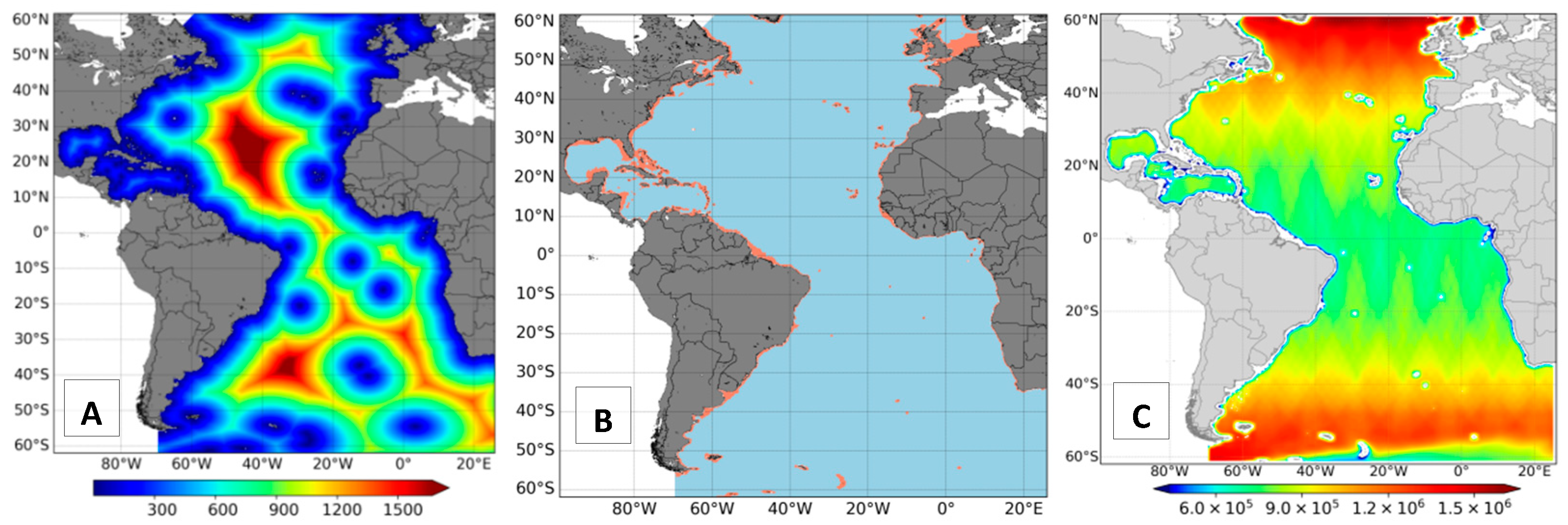
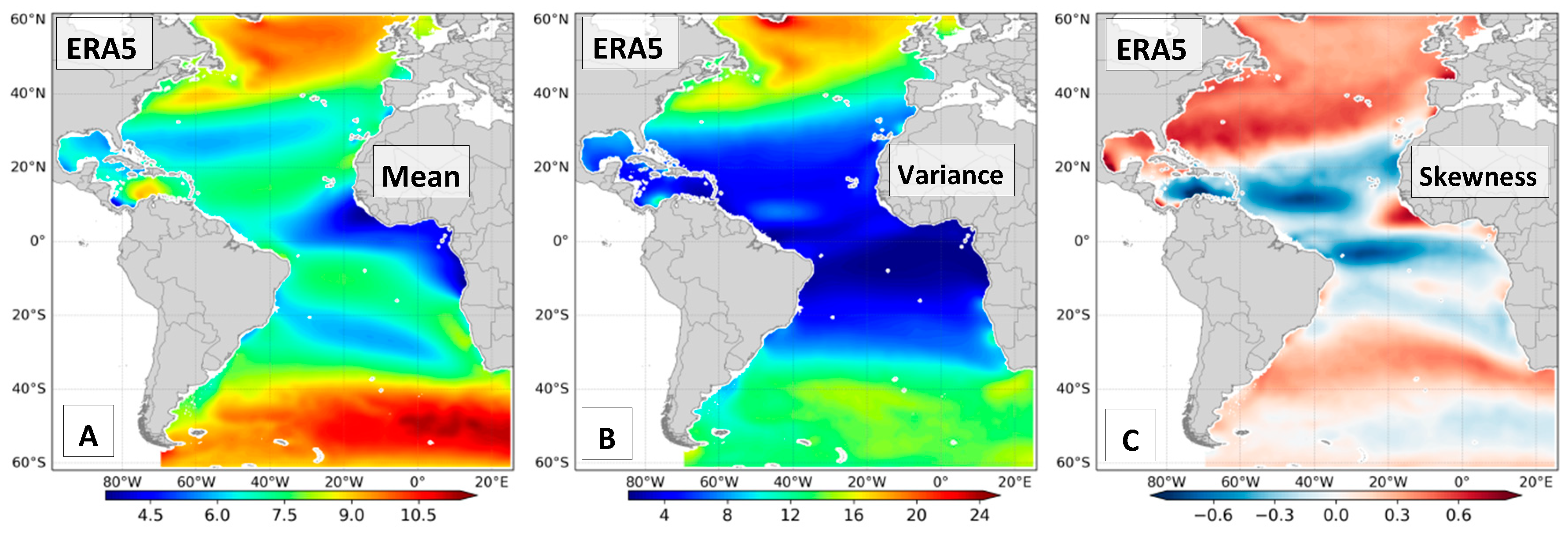
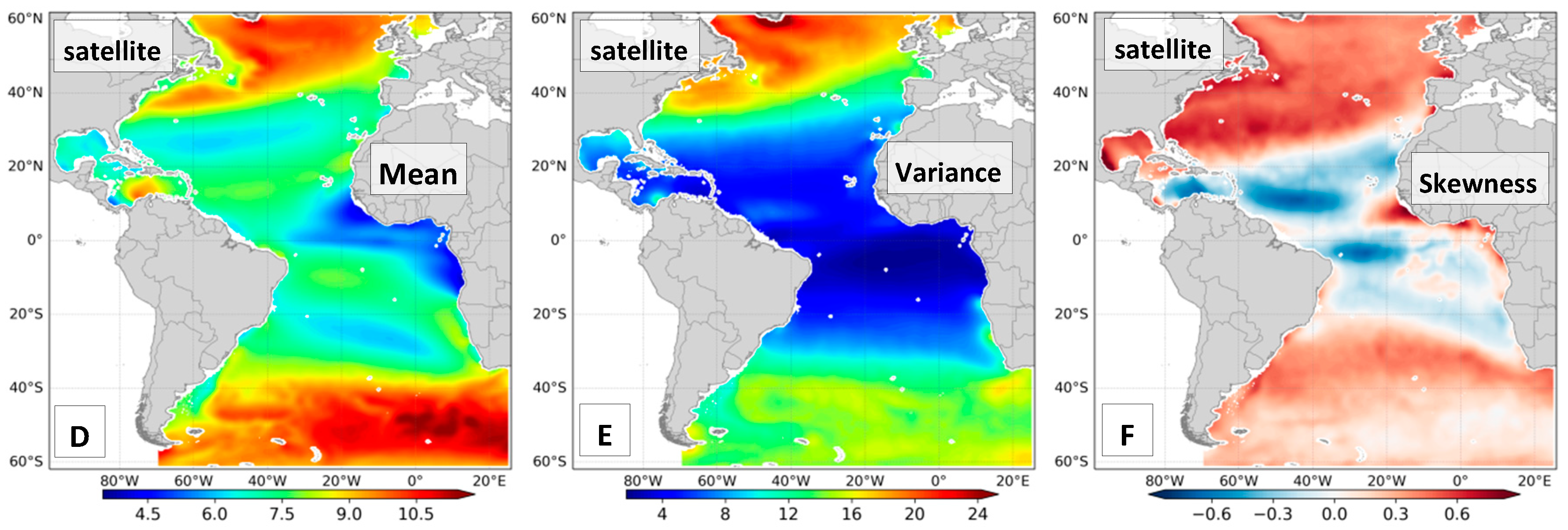
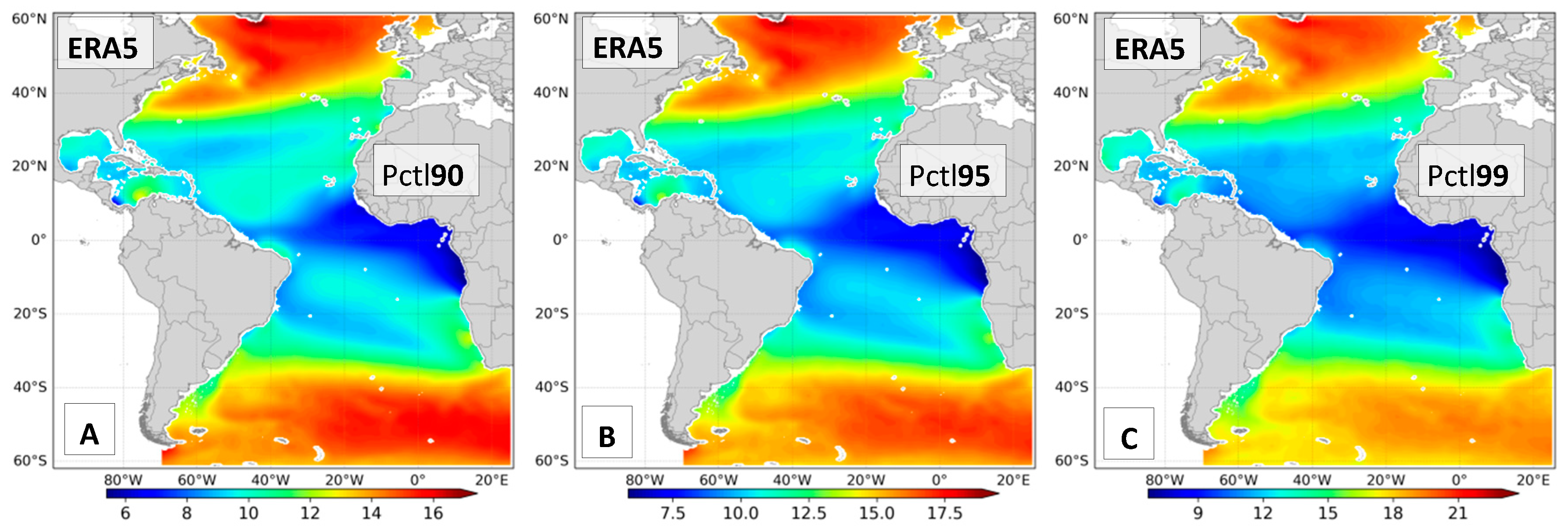
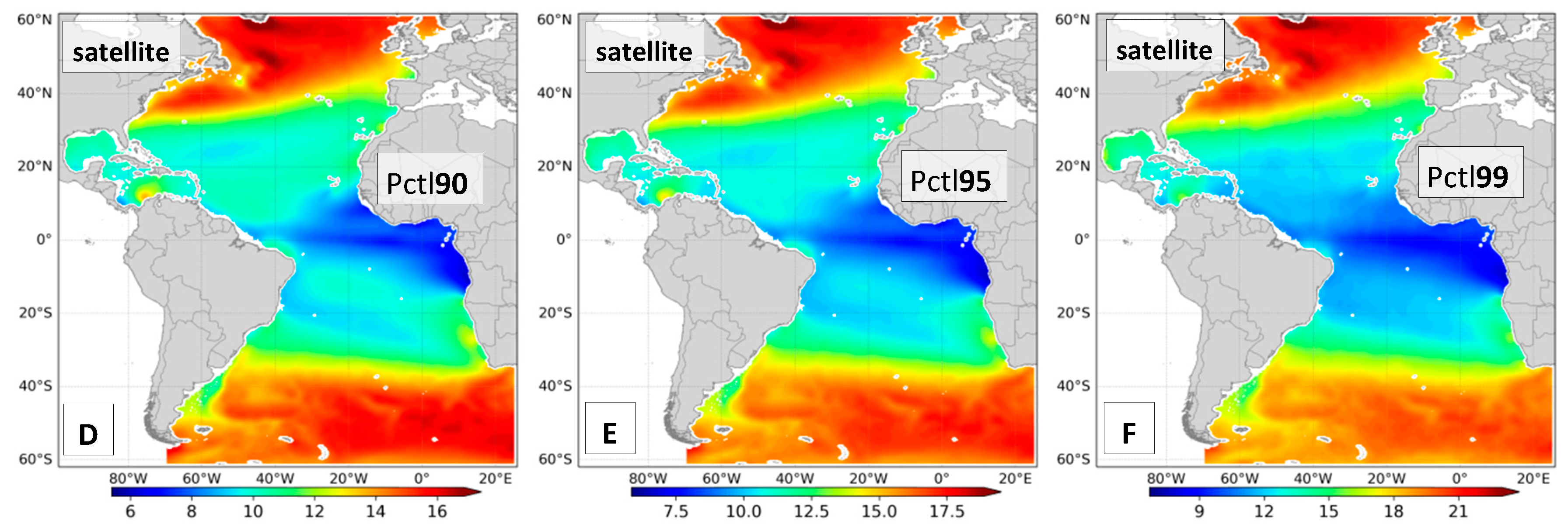
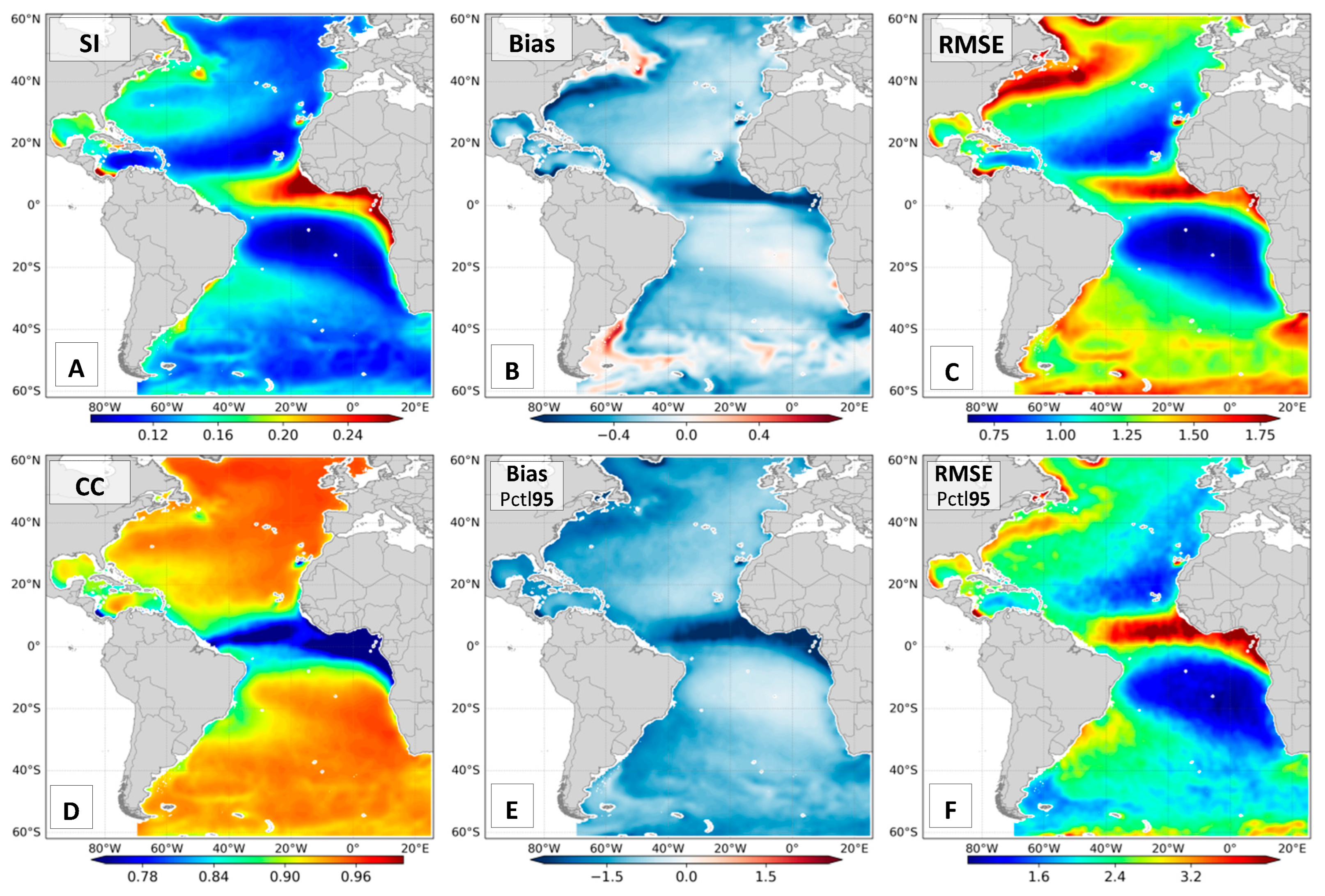
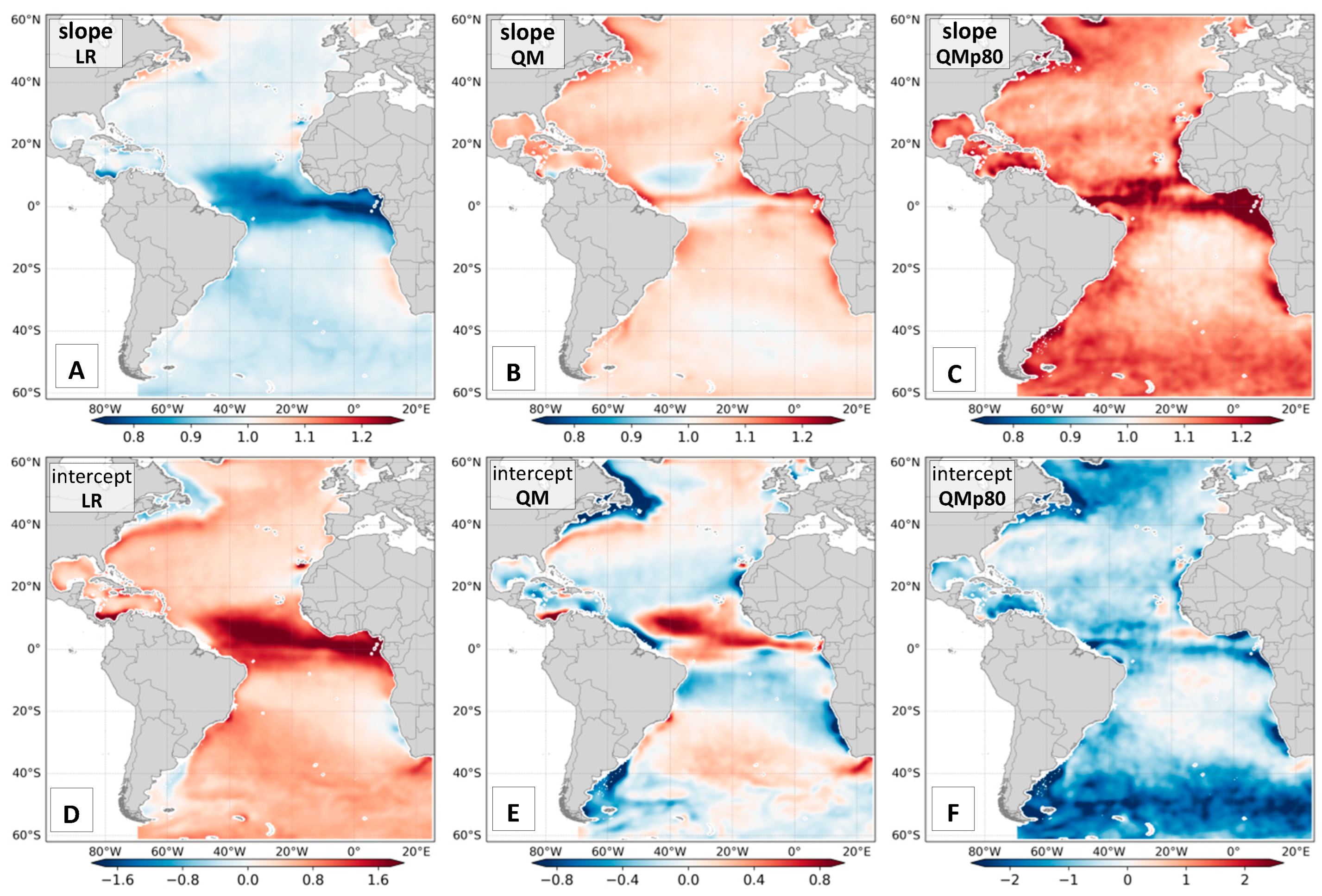
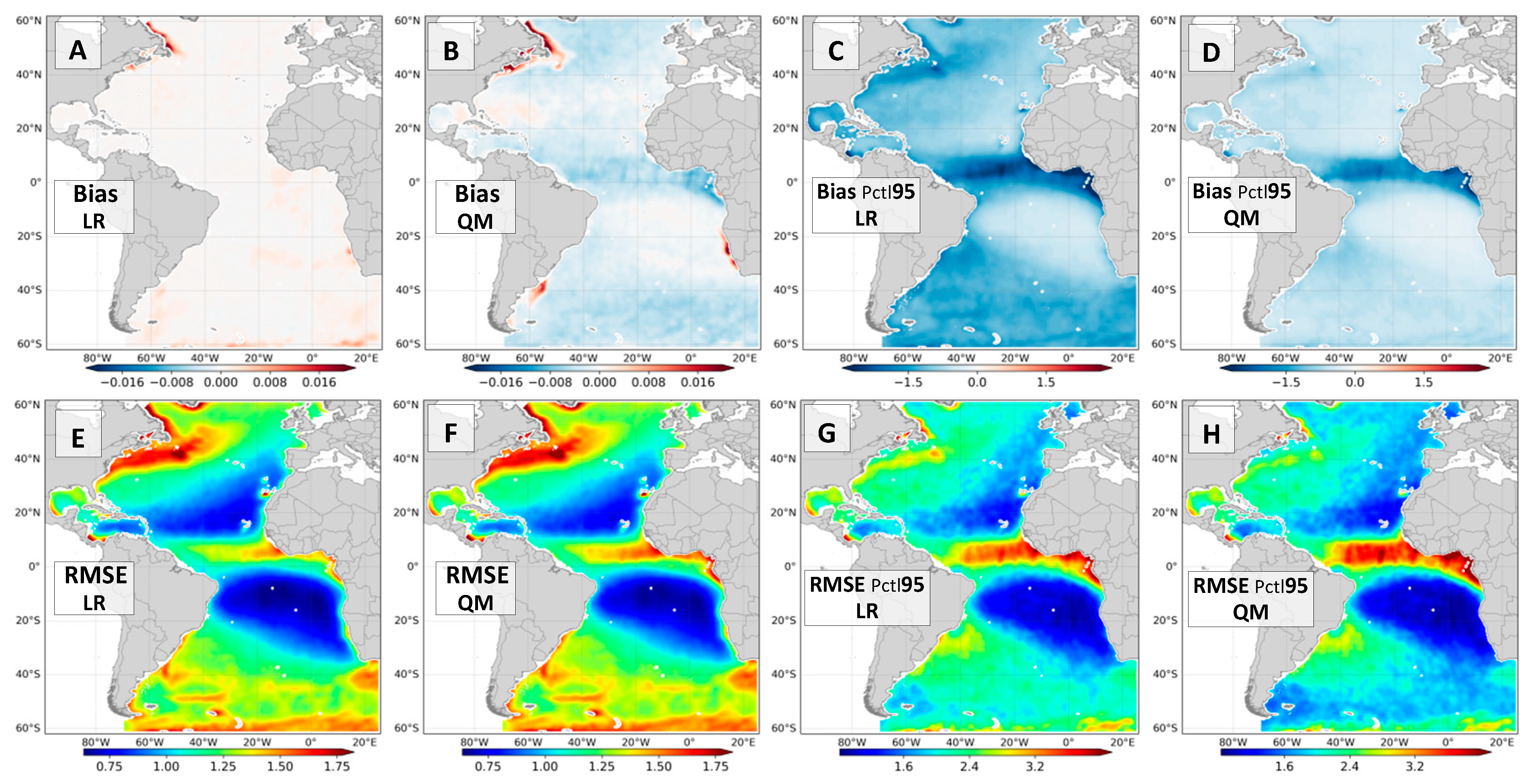
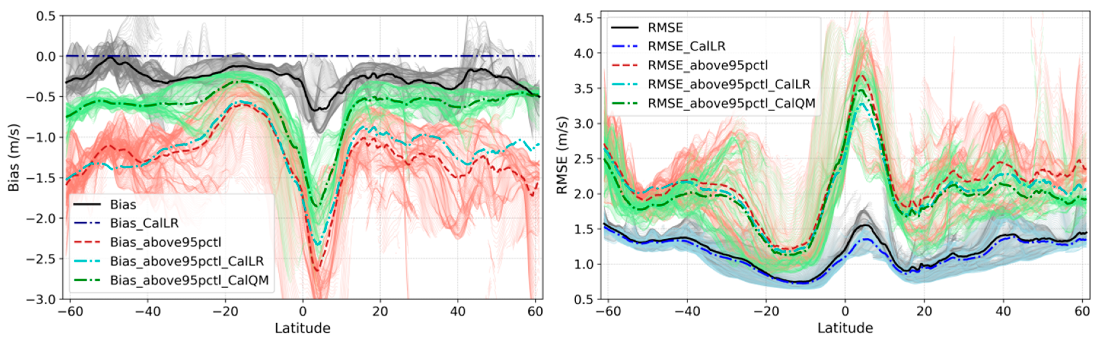
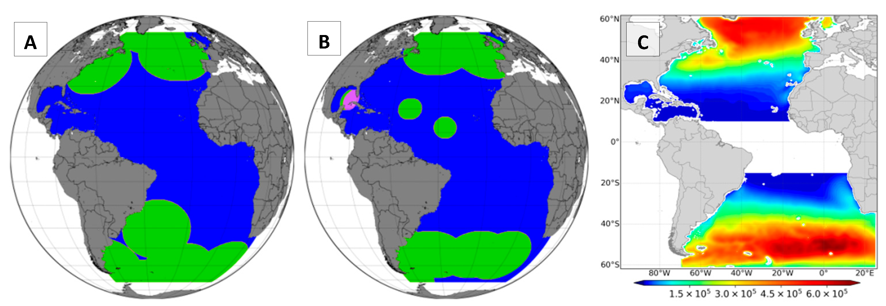
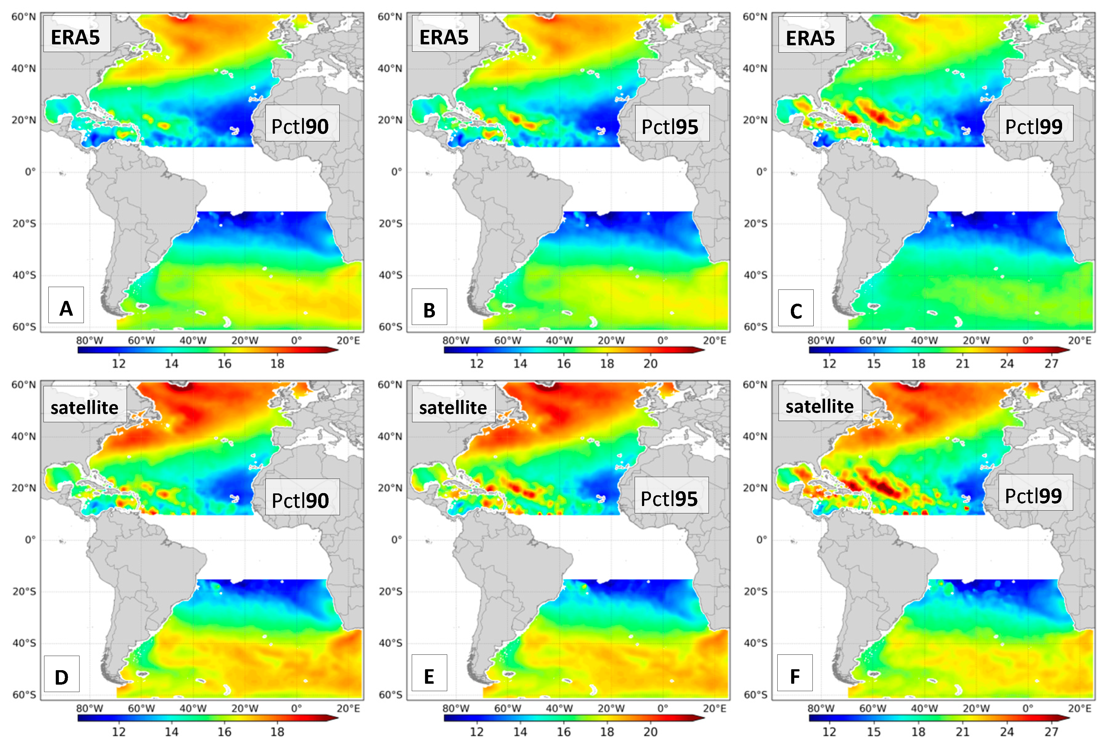
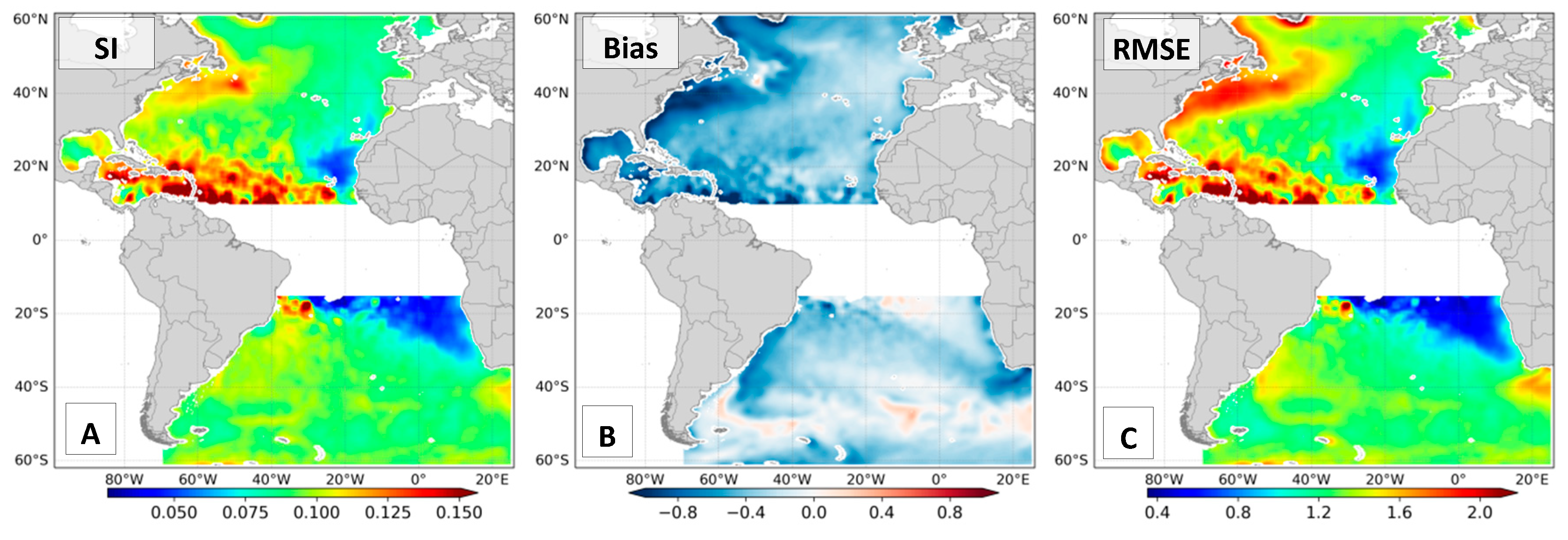
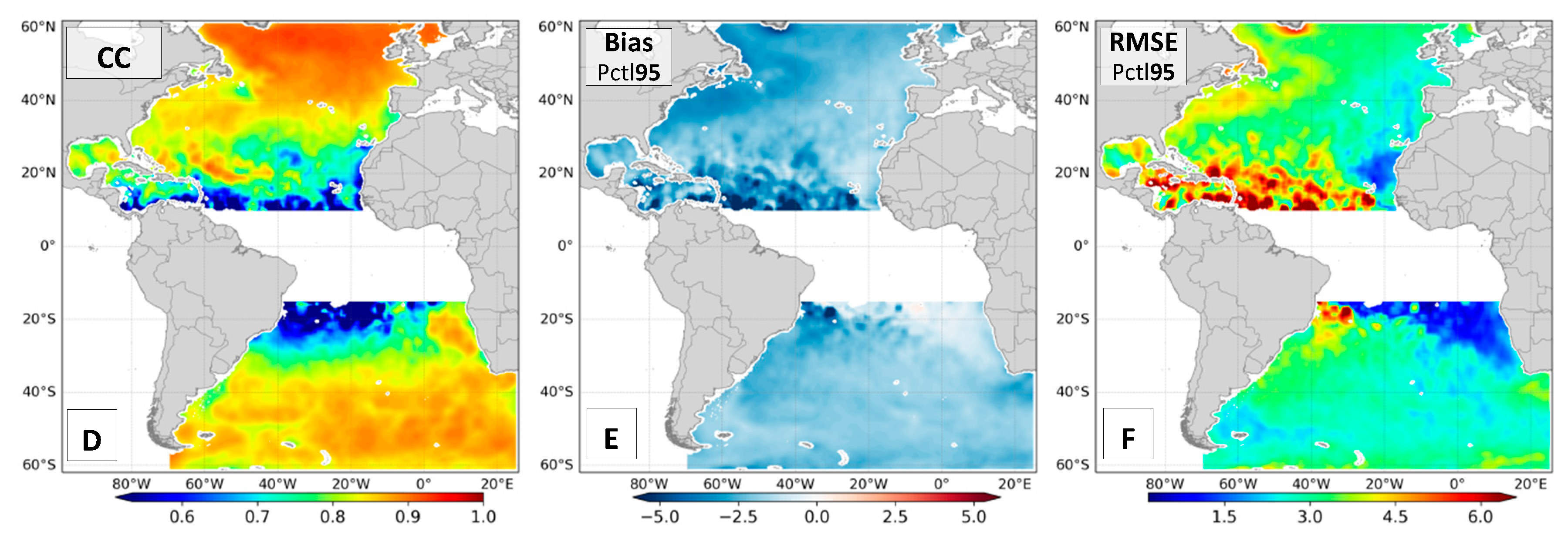
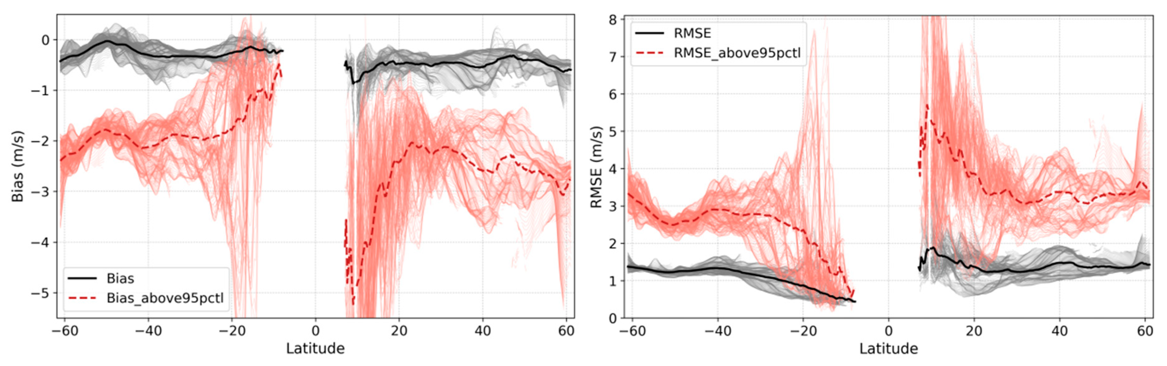
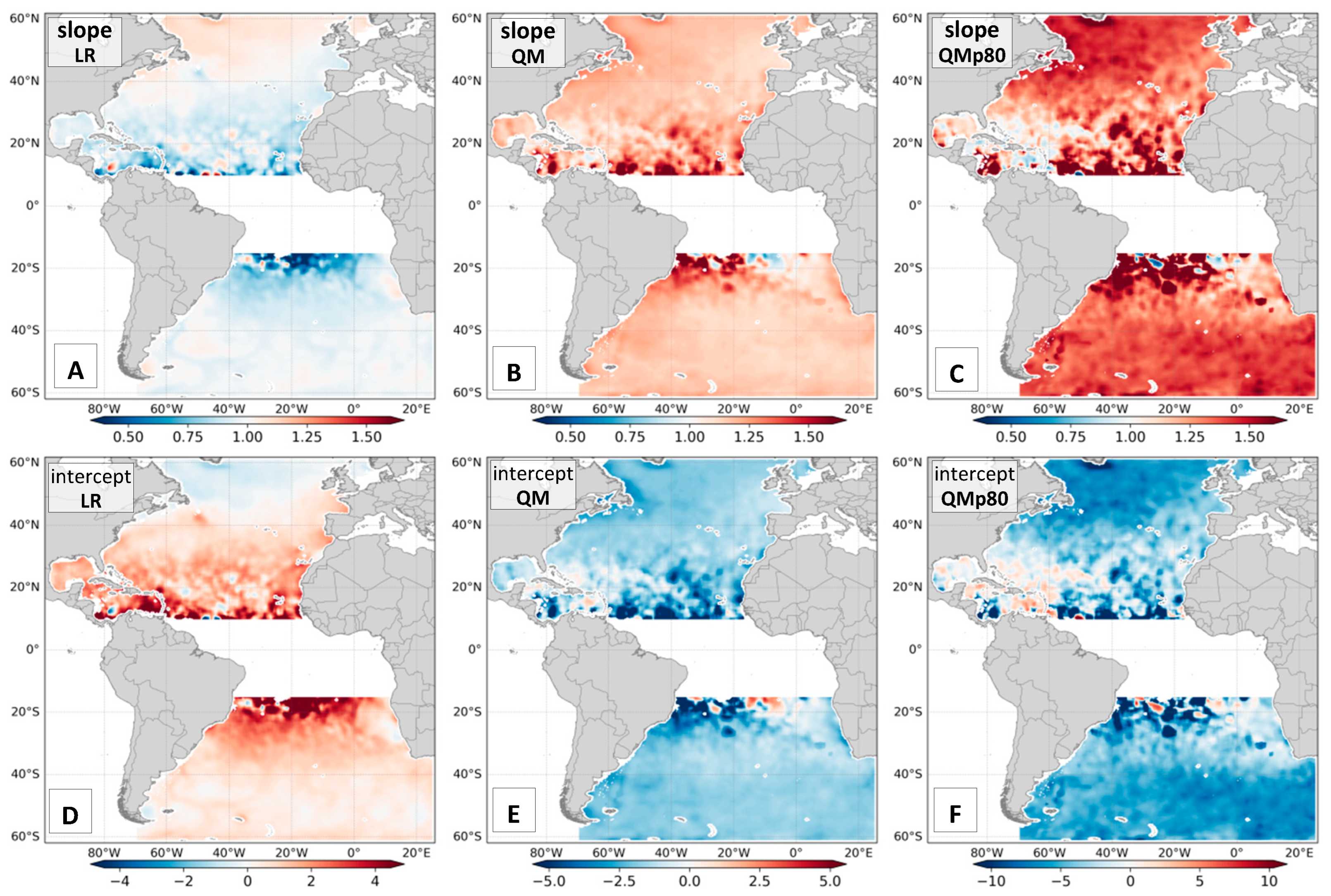
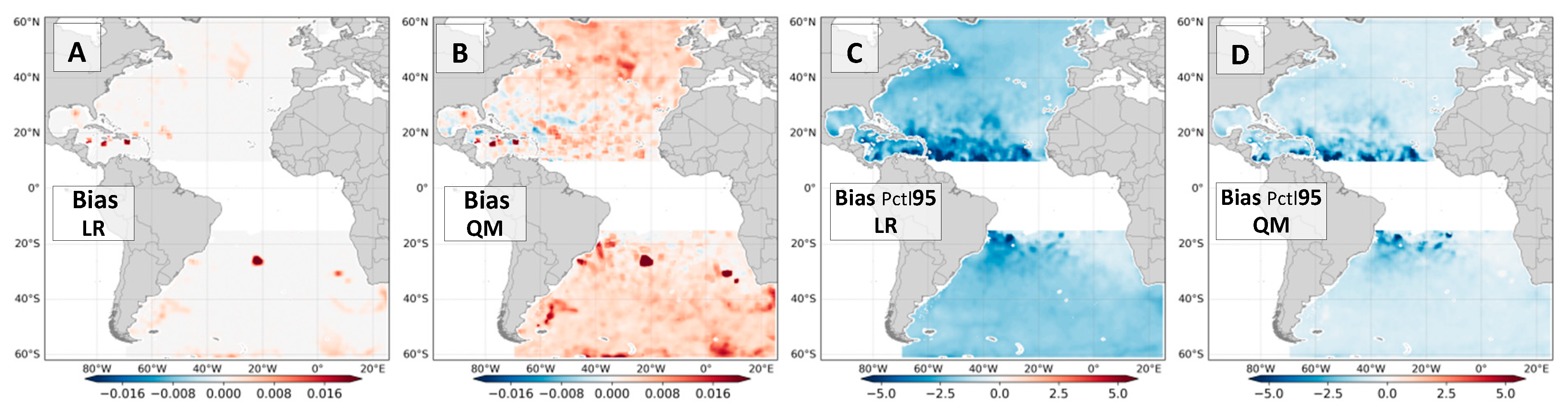
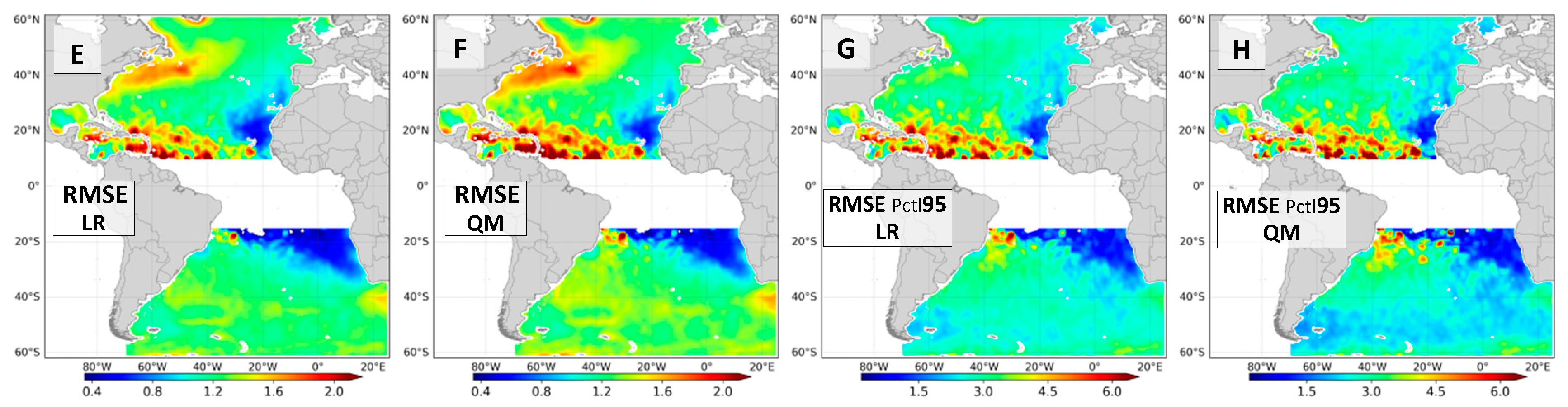
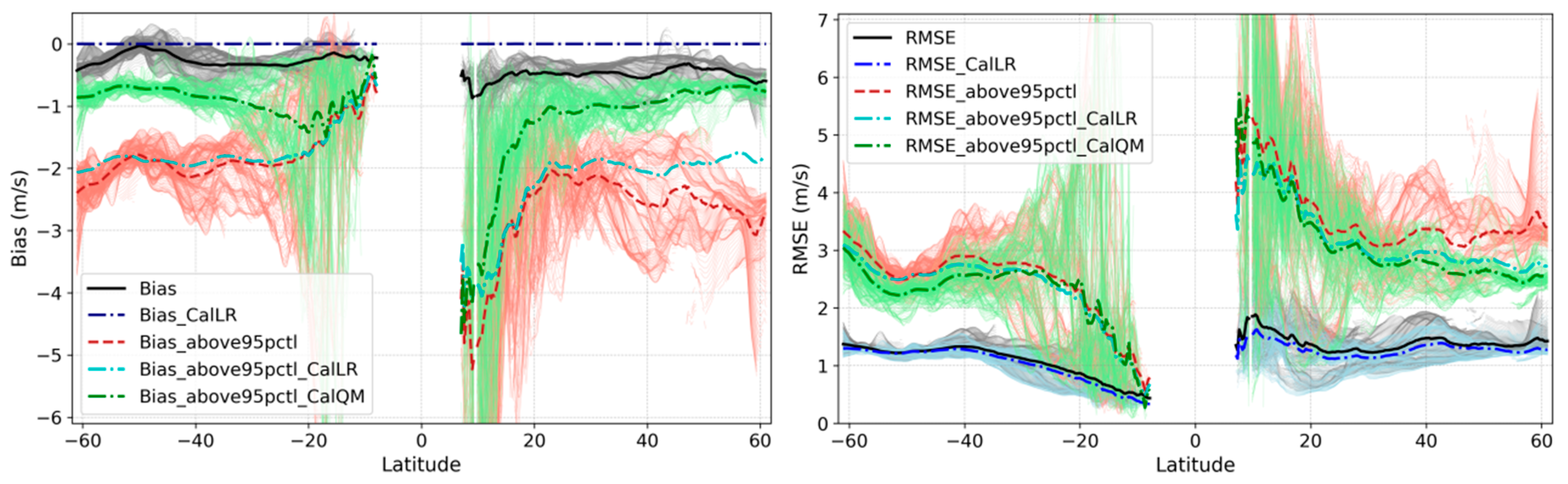
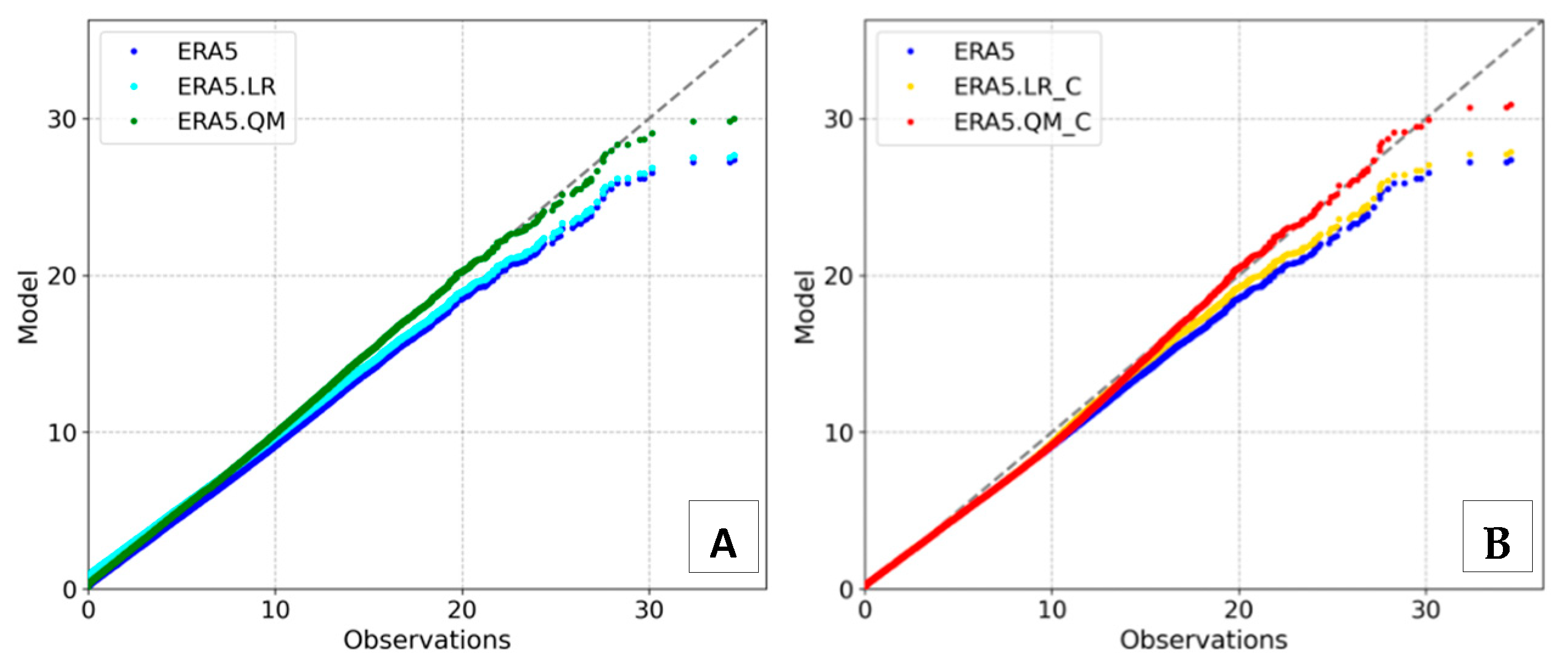
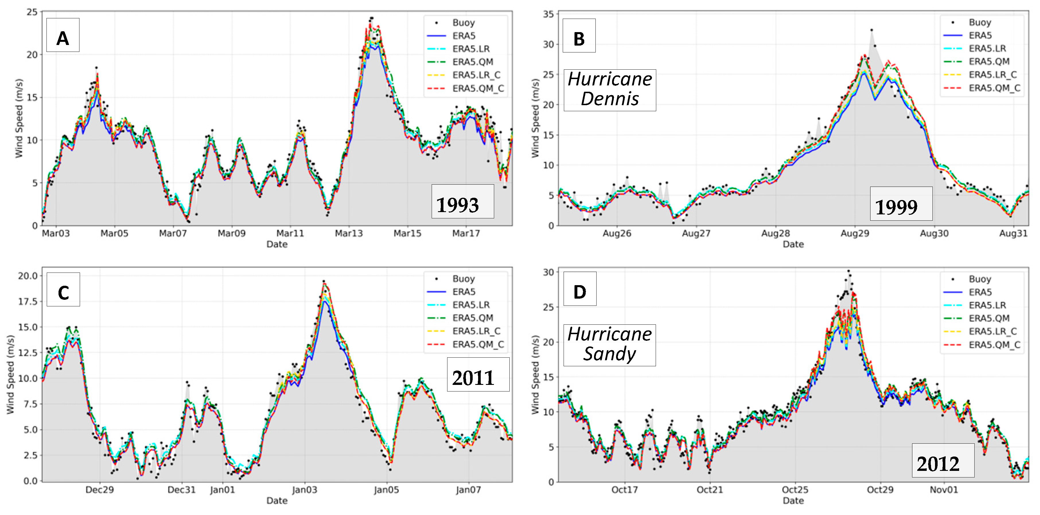
Table 1.
Error metrics (Equations (1)–(4)) calculated for the ERA5 wind speed product and calibration results at the position of NDBC buoy 41,010. The two bottom lines are calibrations performed under cyclonic conditions exclusively. The two right columns are associated with intensities above 20 m/s.
| Bias | RMSE | SI | CC | Bias (U > 20) | RMSE (U > 20) | |
|---|---|---|---|---|---|---|
| ERA5 | −0.487 | 1.366 | 0.173 | 0.919 | −3.642 | 5.257 |
| ERA5.LR | 0.075 | 1.281 | 0.173 | 0.919 | −3.247 | 4.961 |
| ERA5.QM | 0.060 | 1.289 | 0.174 | 0.919 | −1.861 | 4.514 |
| ERA5.LR_C | −0.416 | 1.316 | 0.169 | 0.923 | −3.005 | 4.794 |
| ERA5.QM_C | −0.436 | 1.352 | 0.173 | 0.919 | −1.685 | 4.719 |
Publisher’s Note: MDPI stays neutral with regard to jurisdictional claims in published maps and institutional affiliations. |
© 2022 by the authors. Licensee MDPI, Basel, Switzerland. This article is an open access article distributed under the terms and conditions of the Creative Commons Attribution (CC BY) license (https://creativecommons.org/licenses/by/4.0/).
Share and Cite
MDPI and ACS Style
Campos, R.M.; Gramcianinov, C.B.; de Camargo, R.; da Silva Dias, P.L. Assessment and Calibration of ERA5 Severe Winds in the Atlantic Ocean Using Satellite Data. Remote Sens. 2022, 14, 4918. https://doi.org/10.3390/rs14194918
AMA Style
Campos RM, Gramcianinov CB, de Camargo R, da Silva Dias PL. Assessment and Calibration of ERA5 Severe Winds in the Atlantic Ocean Using Satellite Data. Remote Sensing. 2022; 14(19):4918. https://doi.org/10.3390/rs14194918
Chicago/Turabian StyleCampos, Ricardo M., Carolina B. Gramcianinov, Ricardo de Camargo, and Pedro L. da Silva Dias. 2022. "Assessment and Calibration of ERA5 Severe Winds in the Atlantic Ocean Using Satellite Data" Remote Sensing 14, no. 19: 4918. https://doi.org/10.3390/rs14194918
Note that from the first issue of 2016, this journal uses article numbers instead of page numbers. See further details here.