
Retrieving Water Quality Parameters from Noisy-Label Data Based on Instance Selection
by
 , and
, and
Yuyang Liu
1,2,
Jiacheng Liu
1,2,
Yubo Zhao
1,
Xueji Wang
1,
Shuyao Song
1,2,
Hong Liu
1 and
Tao Yu
1,2,* 1
Key Laboratory of Spectral Imaging Technology, Xi’an Institute of Optics and Precision Mechanics, Chinese Academy of Sciences, Xi’an 710119, China
2
School of Optoelectronics, University of Chinese Academy of Sciences, Beijing 100049, China
*
Author to whom correspondence should be addressed.
Remote Sens. 2022, 14(19), 4742; https://doi.org/10.3390/rs14194742
Submission received: 10 August 2022
/
Revised: 14 September 2022
/
Accepted: 15 September 2022
/
Published: 22 September 2022
(This article belongs to the Section Environmental Remote Sensing)
Abstract
:As an important part of the "air–ground" integrated water quality monitoring system, the inversion of water quality from unmanned airborne hyperspectral image has attracted more and more attention. Meanwhile, unmanned aerial vehicles (UAVs) have the characteristics of small size, flexibility and quick response, and can complete the task of water environment detection in a large area, thus avoiding the difficulty in obtaining satellite data and the limitation of single-point monitoring by ground stations. Most researchers use UAV for water quality monitoring, they take water samples back to library or directly use portable sensors for measurement while flying drones at the same time. Due to the UAV speed and route planning, the actual sampling time and the UAV passing time cannot be guaranteed to be completely synchronized, and there will be a difference of a few minutes. For water quality parameters such as chromaticity (chroma), chlorophyll-a (chl-a), chemical oxygen demand (COD), etc., the changes in a few minutes are small and negligible. However, for the turbidity, especially in flowing water body, this value of it will change within a certain range. This phenomenon will lead to noise error in the measured suspended matter or turbidity, which will affect the performance of regression model and retrieval accuracy. In this study, to solve the quality problem of label data in a flowing water body, an unmanned airborne hyperspectral water quality retrieval experiment was carried out in the Xiao River in Xi’an, China, which verified the rationality and effectiveness of label denoising analysis of different water quality parameters. To identify noisy label instances efficiently, we proposed an instance selection scheme. Furthermore, considering the limitation of the dataset samples and the characteristic of regression task, we build a 1DCNN model combining a self attention mechanism (SAM) and the network achieves the best retrieving performance on turbidity and chroma data. The experiment results show that, for flowing water body, the noisy-label instance selection method can improve retrieval performance slightly on the COD parameter, but improve greatly on turbidity and chroma data.
1. Introduction
At present, unmanned airborne hyperspectral retrieving method [1,2,3,4,5,6] is popular, because the unmanned aerial vehicle has the advantages of quick response, convenient acquisition of spectral data, unlimited detection area, and the capability of retrieving non-point source concentration. This kind of method is suitable for fast surface source monitoring tasks in small water area.
Previous studies [1,7,8,9,10] have shown that when light enters the water, it will be scattered and absorbed by suspended substances and various particles in the water, which will lead to the change of the outgoing light intensity. When the quantity of the water body changes, the proportion of light scattering and absorption by particles in water will also change, so the spectral reflectance curve can be measured to retrieve the quantity parameters of the water body.
According to the state-of-the-art research, unmanned airborne hyperspectral measurement of water quality parameter usually utilize UAV to acquire hyperspectral data. In the meanwhile, portable sensors are carried to measure water quality parameters at sampling points in real time [1,2,3,11,12], or water samples are collected in containers and then sent to chemical laboratory for measurement [4,5,13]. These two schemes to acquire water quality data of sampling points can work in good function in most situations. In practice, due to the UAV speed and route planning, the actual sampling time and the UAV passing time cannot be guaranteed to be completely synchronized, and there will be several minutes difference. There is ordinarily limited change for most of water parameters in several minutes such as chroma, COD, and chl-a, etc. However, for turbidity and suspended solids, especially for a flowing river, the value may change within a certain range. In other words, in the process of turbidity measurement while flying UAV, it is easy to introduce error, which leads to the noisy pollution of the true label value.
When noise error is introduced into the label, the number of outliers may increase. We need to build a more complex model to fit the data which are polluted by noise. This phenomenon has a negative impact on the accuracy and generalization of the model.
We can roughly categorize the methods of processing noisy-label data into two aspects: establishing a robust model against noise [14,15,16] and detecting the noisy instances [17,18,19]. Robust algorithms focus on establishing a robust model, robust loss function against noisy labels rather than identifying specific noisy instances. Noisy label detection algorithms aim to identify noisy data and use a different strategy to deal with the identified noisy data. Numerous patterns are designed to distinguish specific noisy-label data including large error [20], disagreement with nearest neighbors [17]. As for identified noisy data, different strategies are adopted such as discarding [18,19,20], re-labeling [21], or regarding them as unlabeled data in the semi-supervised manner [22], etc.
According to our experiment, we find out that when the water quality parameters are retrieved based on the unmanned airborne hyperspectral method, especially for the flowing water body and the water quality parameters which are easy to change (such as turbidity and suspended solids), an unpredictable error may be introduced in the measurement, resulting in poor retrieving performance. To alleviate the impact, we propose an enhanced Edited Nearest Neighbor for regression (RegENN) instance selection scheme combining modified loss function and hyper-parameter searching strategy to identify noisy-label instance effectively. After noisy instance selection processing, we first analyze the spectral characteristic of three water quality parameters (chromaticity, turbidity and COD). Then, we adopt intelligent algorithms to retrieve these three parameters including Partial Least Squares Regression (PLSR) [23], Random Forest Regression (RFR) [24], K-Nearest Neighbor (KNN) [25], Adaboost [26,27] and our constructed 1D convolutional neural network (1DCNN) model combined with Self Attention module [28,29]. The experiment results show that the band correlation of turbidity parameters in infrared and red region bands is obviously improved after selecting noisy samples, which accords with the prior knowledge of related research [1,3,10]. Meanwhile, for the two relatively stable water quality parameters, chromaticity and COD, the band correlation is not obviously improved, which also indicates that the turbidity measurement data are prone to be introduced to error. Furthermore, the results of modeling and retrieving of the three water quality parameters show that, after noisy label selection processing, for turbidity, R2 and mean absolute error (MAE) on test dataset modeling by PLSR, RFR, Adaboost and 1DCNN all have various promotion. While for other two parameters, chroma and COD, R2 and MAE on the test dataset is not obviously improved after noisy label instance selection.
Contributions. Our contributions are listed as follows:
- In case of label-noisy problems for flowing water, an enhanced RegENN instance selection scheme is proposed to identify noisy label instances;
- Experiments on the retrieval of turbidity, chroma and COD are conducted to verify the necessary of noisy-label instance selection for the turbidity parameter;
- Experiment results on retrieval of turbidity, chroma and COD show that it is easy to introduce label noise to turbidity and chroma, while COD is more stable; and
- The 1DCNN network combining Self Attention module is proposed for regression. The network achieves the best retrieving results on turbidity and chroma data.
2. Materials and Methods
2.1. Data Acquisition
2.1.1. Study Area
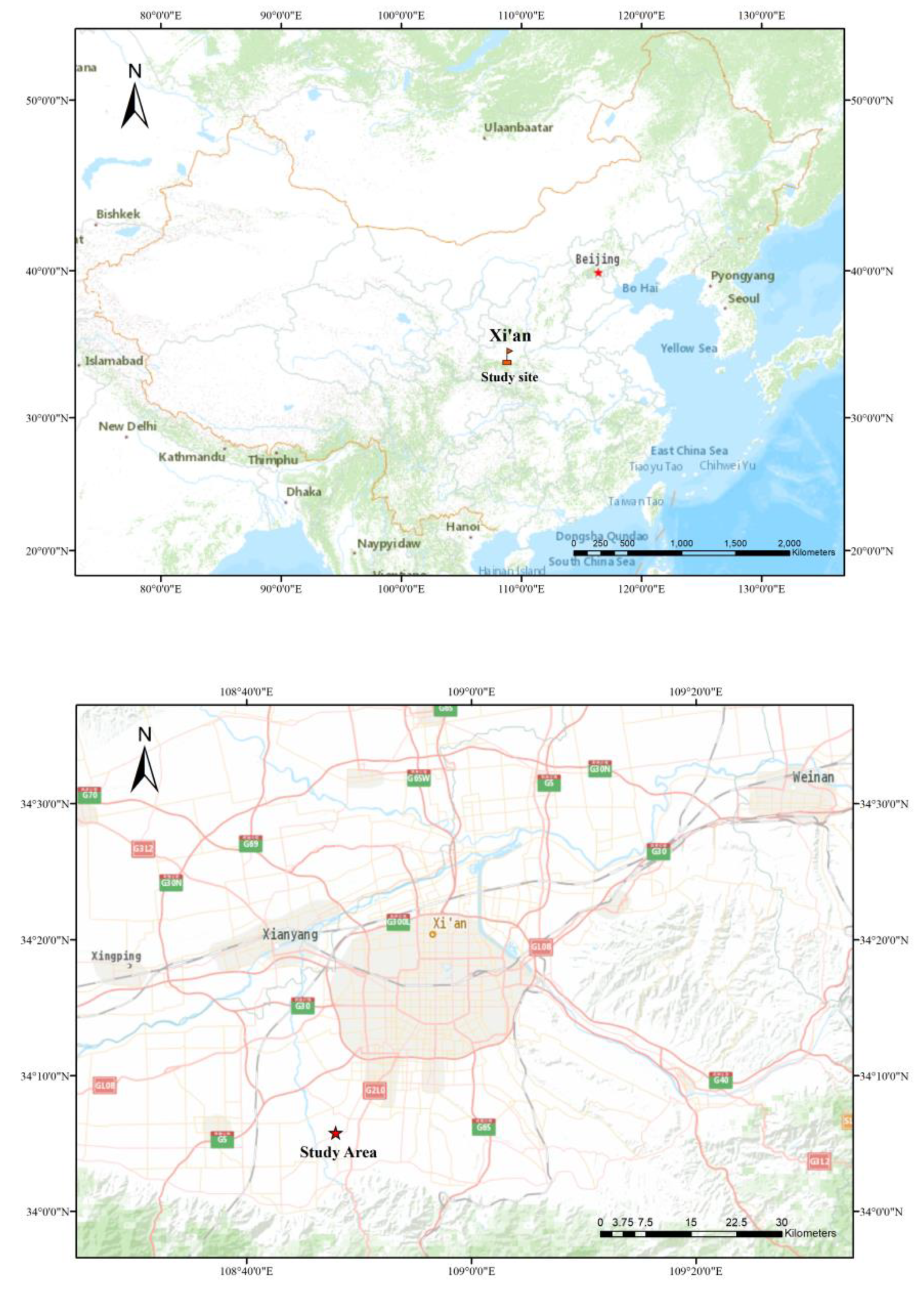
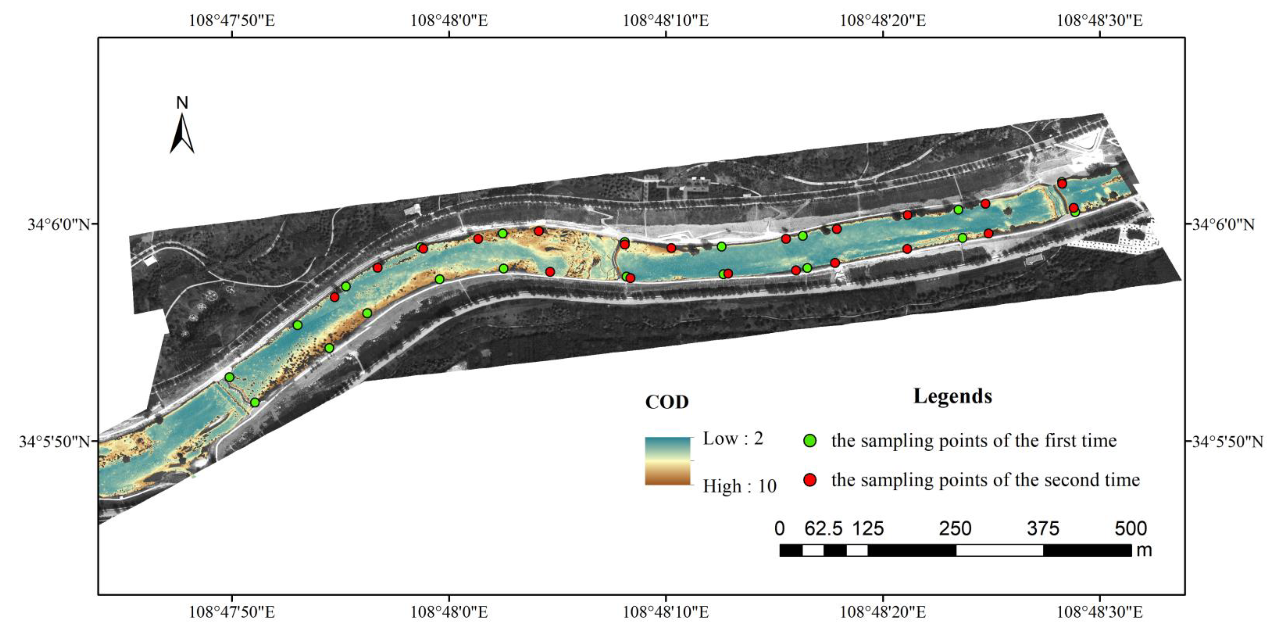
The study area was selected as the Xiao River Ecological Park in Xi’an, Shaanxi Province, China. The experiment was conducted on 28 March and 11 April 2022. The weather in the experiment was sunny and wind was Level 2. This experiment covers a river length of 1.1 km. Sampling points are set at intervals of about 50 m. There are 40 groups of sampling points in total. However, four samples are corrupted by the shadow of trees and abandoned. The final 36 samples are divided into 28 samples for training model and 8 samples for testing. The sampling points and experimental areas are shown in Figure 1 and Figure 2. Figure 2 is the COD inversion map with the actual sampling sites on 11 April.
2.1.2. Water Sampling and Measurement
When the UAV is performing a flight task, we take water samples at the same time. We recorded the latitude and longitude information and photographed the landform of the sampling points while measuring the water quality parameters. The water quantity parameters are measured by portable sensors. Limited by the instrument, three water parameters were measured including chroma, turbidity and COD. The turbidity is measured by Hach 2100Q with 0.01 NTU resolution. The COD is measured by INESA COD-571 analyzer with 8%FS resolution. Chromaticity is measured by Hach LICO620 chroma analyzer. At every sampling point, we measured the parameters 5 times and recorded the average value. The values of chroma range from 32.07 to 69.67 Hazen. The values of turbidity range from 3.33 to 12.51 NTU. The values of COD range from 2.22 to 9.49 mg/L. Detailed statistics of the data set are shown in the Table 1.
2.1.3. UAV Hyperspectral Image Acquisition
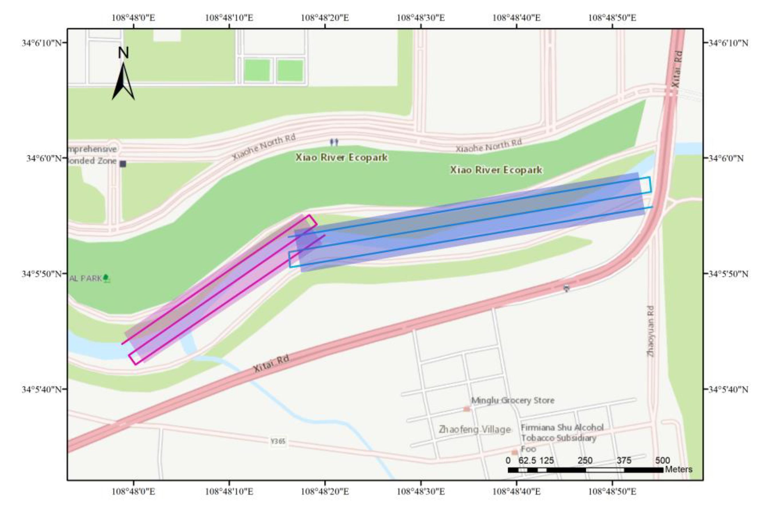
We use the DJI Wind 4 UAV, which weighs 7.3 kg, has a maximum load of 24.5 kg and a maximum flight speed of 14 m/s. Corning Micro HSI410 model is adopted for collecting hyperspectral images. This type of hyperspectral imager is a push-scan imager, with an effective detection range from 400 to 1000 nm and a spectral interval of 4 nm, with a total of 150 bands. Considering the mosaic of image strip, the lateral overlap is set to 40%. Due to the curvature of the river, the flight was completed twice to cover the full area of the experimental site. Considering the time interval between the two flight tasks and the change of light conditions, the standard whiteboard and standard grayboard with a reflectance of 70% and 25% and a size of 2 × 2 m were placed in the two flight areas as a reference. The UAV flew at an altitude of 200 m and a flight speed of 10 m/s. The duration of a single flight was less than 10 minutes and the weather was sunny. We assume that in a single flight, the lighting conditions are basically unchanged [30,31,32]. The flight area and route planning are shown in Figure 3.
2.2. Methods
2.2.1. Geometric Correction
Due to the vibration and airflow effects when the drone is flying, the image is tilted and offset, and geometric correction is required [33]. Geometric correction of the original image based on latitude and longitude and inertial guidance information recorded by hyperspectral imager.
2.2.2. Radiation Correction and Spectral Reflectivity
According to radiation transmission theory, the radiance of the target detected by the hyperspectral imager mounted on the drone has two parts. One part is radiation from water, and the other part is diffuse reflection from the sky. Among them, the sky diffuse reflection is radiation information without any water surface information, which needs to be removed. According to [3,5,34], radiance detected by a spectrometer can be expressed as follows:
where is the radiance of departure from water; is the diffuse reflection of the sky without any water information; is the reflectivity of the air–water boundary facing the sky light, which is influenced by various factors such as solar system, observation geometry, wind speed, and etc. the value of can be set in the range of . In a breezy or windless environment, the water surface is calm and is set to 0.022. When the wind speed is about 5 m/s, can be set to 0.025, and when the wind speed is 10 m/s, is set to 0.026–0.028.
In order to calculate the reflectivity of the water surface, the total incident radiation needs to be estimated. According to [3,35], we can place the gray standard board on the waterside ground, and the gray standard plate reflectivity is about 10% to 30%. Then we can estimate the total incident radiance by Equation (2).
where is digital value of the radiance, is the reflectivity of the standard gray board.
Finally, the departure reflectivity of water can be calculated by Equation (3):
2.2.3. Spectral Curve Filtering
Due to the instability of the sensor and the influence of weather factors, hyperspectral data often introduces noise when acquiring, which not only reduces the image quality, but also affects the results of subsequent data processing [36]. To eliminate noise and glitch conditions, we smoothed the spectrum of each pixel using the Savitzky Golay filtering method [37].
2.2.4. Noisy-Label Instance Selection
Given a data set . For regression tasks, according to the regression definition, we can write as:
where is a regression mapping function, is the error of the predicted value and the label value. For data with noisy labels, the label may not be true values, and we assume that the latent true values are , the error between the latent true value and the actual value needs to be considered. We assume the noise error conforms to a normal distribution, then Equation (4) can be written as:
where indicates mean-shift parameter, representing the mean value of the difference between the label value and the latent true value. is random error and . If is non-zero, it means this sample pair may be polluted by noise. Meanwhile, to guarantee the fidelity of the data, we assume that the noisy-label instances are sparse, which can be expressed as:
where k is a parameter indicating maximum noise label threshold. The value of k is usually unknown and related to specific dataset.
For regression problems, the solution objective can be expressed as:
where is a function measuring the distance of a and b, is a sparse loss function. Equation (7) indicates that the number of detected noisy samples should be as small as possible in the case of eliminating noisy label offsets.
To determine appropriate value of , we introduce RegENN algorithm. RegENN is a noisy label sample selection method for regression problems proposed by Kordos [17] et al. The core idea of the RegENN algorithm is that for regression problems, the labels of similar samples should be similar. If the labels of similar instances of the sample to be detected are quite different from its label, the sample to be detected can be considered as a noisy-label instance. The RegENN algorithm can be expressed by pseudocode as the following Algorithm 1.
| Algorithm 1: RegENN: Edited Nearest Neighbor for regression using a threshold |
| Data: Training set , hyper parameter α to control how the threshold is calculated from the standard deviation, the number of neighbors k to train the model. |
| Result: Selected instance set |
In Algorithm 1, we chose Manhattan distance as the metric distance for the nearest neighbor algorithm. Manhattan distance can be formulated as follows:
According to the spectral analysis, we found that the reflectance spectral curves of different water bodies are similar in shape, and more manifested in different amplitudes. So, the SAM measurement method is not suitable. Compared to SAM-based distance measurements, Manhattan distance is more sensitive to spectral reflectance amplitudes. For the search of similar samples of the target sample, we use the K-nearest neighbor method.
However, in the original algorithm, the determination of α is actually a problem. When the value of α is too large, fewer samples will be determined as outliers, and when the value of α is too small, more samples will be determined as outliers, resulting in data distortion. Combining Equation (7) and RegENN, the water quality parameter regression problem can be written as:
where is the model trained after removing noisy label samples, is model fitting error after removing noisy label samples, is a function of the number of noisy samples related to α, is a loss function to detect the number of noisy samples, t is a weight parameter. Our objective is to not only ensure the model fit after noisy label instance selection, but also impose certain constraints on the number of detected samples to ensure data fidelity. For the specific mathematical form of and , we will discuss in the Section 3.1 below.
For the setting of the value of α, we use the grid search method. Empirical values of α given in previous studies ranged from . Within this range, we adopt the grid search method, combined with Equation (9), and determine value of α.
2.2.5. Water Quality Parameter Inversion
We use PLSR, RFR, KNN, Adaboost, 1DCNN-based algorithms to retrieve three water quality parameters (chromaticity, turbidity and COD). As methods are intelligent algorithms, we take all the bands as input and test the performance of different algorithms. The PLSR, RFR, KNN, Adaboost algorithms use functions included in the python programming library scikit-learn.
At the same time, we build a 1DCNN model for further improving the fitting performance. Due to the small number of samples and the large number of spectral bands, in order to better allow the model to learn better features, we introduce the Self Attention module. Self attention mechanism (SAM) is proposed by [38]. Attention mechanism can make a network learn a weight vector that indicates the importance of different features which improves network performance. It can be divided into two categories, spatial attention [39] and channel attention [40]. For hyperspectral data, we adopt channel attention to allow the model to learn better features.
As for loss function, we adopt Smooth L1 loss:
For the regression problem, the Smooth L1 loss not only solves the problem of the gradient explosion caused by the L2 loss for outliers due to the large difference, but also solves the disadvantage that the L1 loss is not smooth enough in the [−1, 1] interval. The 1DCNN network structure we constructed is shown in the Table 2.
2.2.6. Accuracy Assessment
The retrieving accuracy of water quality parameters can be evaluated by the correlation coefficient r, coefficient of determination (R2), MAE, and accuracy (Acc). The formulas of these three evaluation indicators are as follows:
where is label value, is mean of the label value, is predicted value, N is the number of samples, is the number of samples with PE less than 20% [41].
3. Experiments and Results
In this section, we will describe and discuss the experimental results in detail. In Section 3.1, we describe in detail the algorithm parameter settings adopted during the experiments. In Section 3.2, the characteristics of the reflectance spectral curves will be analyzed. At the same time, we compared the spectral correlation differences before and after instance selection. In Section 3.3, the comparison results of the original data set and denoised data set with different inversion algorithms will be shown in the following table. In Section 3.4, for the selection of the threshold parameter ɑ, we conduct experiments on three water quality parameters using the random forest method.
3.1. Experiment Settings
In the process of detecting noisy label data, when the k-neighbor algorithm detects similar spectral samples, following the experienced value proposed by RegENN, the value of k can be set from 4 to 8. In the experiment, we set k to six, that is, using the Manhattan distance as a metric, and select six adjacent samples. A grid search method [42] was used to determine the hyperparameter α, searching from 1 to 30 with a search step of 0.1. The value of the hyperparameter α will vary according to different regression models, and the specific range is shown in the Table 3.
For the selection of , we combine MAE and R2 loss functions, and it can be formulated as . Meanwhile, we define . This will ensure that when the number of noisy instances selected is too large, the loss will increase rapidly, thus limiting the range of . The loss weight parameter t is set to .
The parameter settings of the water quality inversion algorithm are described as follows. The PLSR algorithm uses the five most correlated bands for inversion. The n_estimator and max_depth are two common parameters in RFR and Adaboost algorithms. For the random forest regression algorithm, we set the parameter n_estimator to 100 and the max_depth to 10. For the Adaboost algorithm, we set n_estimator to 50. The number of neighbors in the KNN algorithm is set to six. For our constructed 1DCNN network, the training epoch is set to 800 and the learning rate is set to 0.001.
3.2. Spectral Characteristic Analysis
To inverse water quality parameters, there are several methods such as band math method and intelligent method. For the band math method, it is important to find the most correlated bands to formulate. To evaluate the correlation of different bands, correlation coefficient is a statistical indicator that reflects the relationship between variables. The promotion of coefficient makes it easier to find suitable spectral bands to formulate.
Figure 4 shows band correlation curves for three water quality parameters. As shown in the figure, for the turbidity variable, there is a strong correlation between the blue light band in the range of 400–500 nm and the near-infrared band in the range of 720–850 nm, which is consistent with the prior knowledge [1,8,10]. For the chromaticity variable, there is a strong correlation in the visible light band in the range of 400–800 nm. For COD variable, there is no significant band correlation for the overall spectrum, as expected. Because COD has no obvious optical signature on the reflectance spectrum, the underlying relationship needs to be further explored [10,43].
After the process of instance selection, it can be found that the band correlation of turbidity has been significantly improved, while the band correlation of chromaticity and COD has not been significantly improved. It can be concluded from the experimental results of spectral correlation that there is a more obvious label noise effect on the turbidity data. This experimental result verifies our idea to some extent that turbidity is more prone to introduce noise due to its characteristics.
3.3. Water Quality Parameter Retrieving Results
In the previous section, we analyzed the band correlation of the reflectance spectrum, but only illustrated the improvement in the linear relationship of the data. In this section, we retrieve three water quality parameters using several currently popular intelligent regression methods. In the experiments, we used the divided 28 samples for training model and eight samples for testing. The experimental results are shown in the Table 4, Table 5 and Table 6.
Table 4 shows the results of turbidity inversion using the above method. From the results, it can be found that our constructed 1DCNN network achieves the best results. The model was trained on the original data set and the denoised data set, and achieved R2 of 0.873 and 0.904 on the test set, and MAE of 0.114 and 0.084, respectively. After denoising of the training set, except for the PLSR method, other methods have obvious improvements in the test set R2 and MAE. Among them, the KNN method improved from 0.335 to 0.634 on the test set R2, the largest improvement. However, due to the poor fitting performance of the KNN regression method, the R2 on training set only increased from 0.321 to 0.461, and did not achieve good fitting performance. Except for the KNN method, the RFR method achieves the largest performance improvement after denoising the training set. The RFR method improves from 0.73 to 0.844 on the test set R2 and from 0.208 to 0.144 on the test set MAE. Parameter n represents the number of noisy label instances detected when the model achieves the best performance. For the turbidity data, the number of noisy instances detected varies from five to eight, depending more on the regression model used.
Table 5 shows the results of different methods for chroma inversion. The 1DCNN method achieves the best performance on the test set. On the original dataset, the R2 and MAE on test set are 0.834 and 0.096. After denoising on the training set, the R2 and MAE of the 1DCNN method on the test set are 0.877 and 0.093, respectively. After the denoising of the training set, the R2 and MAE of these methods on the training set have a certain improvement, but the R2 and MAE on the test set are not significantly improved or even have a certain decline. Furthermore, after the denoising of the training set, the R2 of the 1DCNN method is improved from 0.834 to 0.877. The KNN method has improved on the training set, but the performance on the test set has decreased. The number of detected noisy instances varies from one to three, significantly smaller than the value of n for the turbidity data. We assume that there is less noise in the chroma data, and removing the detected outlier samples will significantly improve the performance on the training set. However, since these outliers are difficult to learn samples, not noisy samples, the model will learn an incomplete feature extraction, so the improvement of R2 and MAE is not obvious or even decreased on the test set.
Table 6 shows the results of different methods for COD inversion. For retrieving COD, although the R2 of 1DCNN on the training set is very high, the R2 performance on the test set is not as good as other intelligent methods, whether the training set has been denoised or not. We suppose this is because the neural network model is not able to learn the correct feature representation. Since the relationship between COD and reflectance spectrum is not as obvious as turbidity and chromaticity, the limited amount of data makes the neural network unable to learn effective feature representation. Furthermore, Adaboost achieves the best performance in inversion of COD experiment. On the original dataset, the Adaboost method achieves R2 and MAE of 0.574 and 0.089 on the test set, respectively. After denoising on the training set, R2 and MAE of test set reach 0.662 and 0.078, respectively. Overall, the model cannot perform as well on the test set as chromaticity and turbidity, since COD does not have a particularly distinct feature on the reflectance spectrum. It should be noted that due to the poor fitting performance of KNN, and even an expected fitting performance cannot be obtained on the training set, subsequent experiments were not carried out. In the COD inversion experiment, the Adaboost and 1DCNN methods have significantly improved R2 on the test set after denoising. However, after the instance selection, the fitting ability of other methods on training set is reduced. For RFR and PLSR methods, after the instance selection, R2 on the training set drops from 0.847 to 0.817, and from 0.634 to 0.603, respectively. The model did not fit the data well in the training set, and the results on the test set are definitely not as expected. Besides, the number of detected noisy instances varies from one to two, which is less than the number of noisy instances detected on turbidity data.
According to the Table 4, Table 5 and Table 6, we found that when the number of selected noisy instances is between five and eight, the model for turbidity inversion will have a more obvious performance improvement. The turbidity results show that it is easier to introduce label noise into turbidity data for flowing water body. When the number of selected instances is two to three, the inversion chroma model will have a certain performance improvement, but the magnitude is not large, which indicates that less label noise is introduced into chromaticity data for flowing water body. However, after the instance selection of COD, the performance is not significantly improved or even dropped. It could be concluded from the results that the value of turbidity changes quicker than COD in the flowing water body and it accords with our actual experience while measuring. For turbidity and chromaticity parameters, our methods obtain expected performance improvement.
3.4. Parameter Experiment
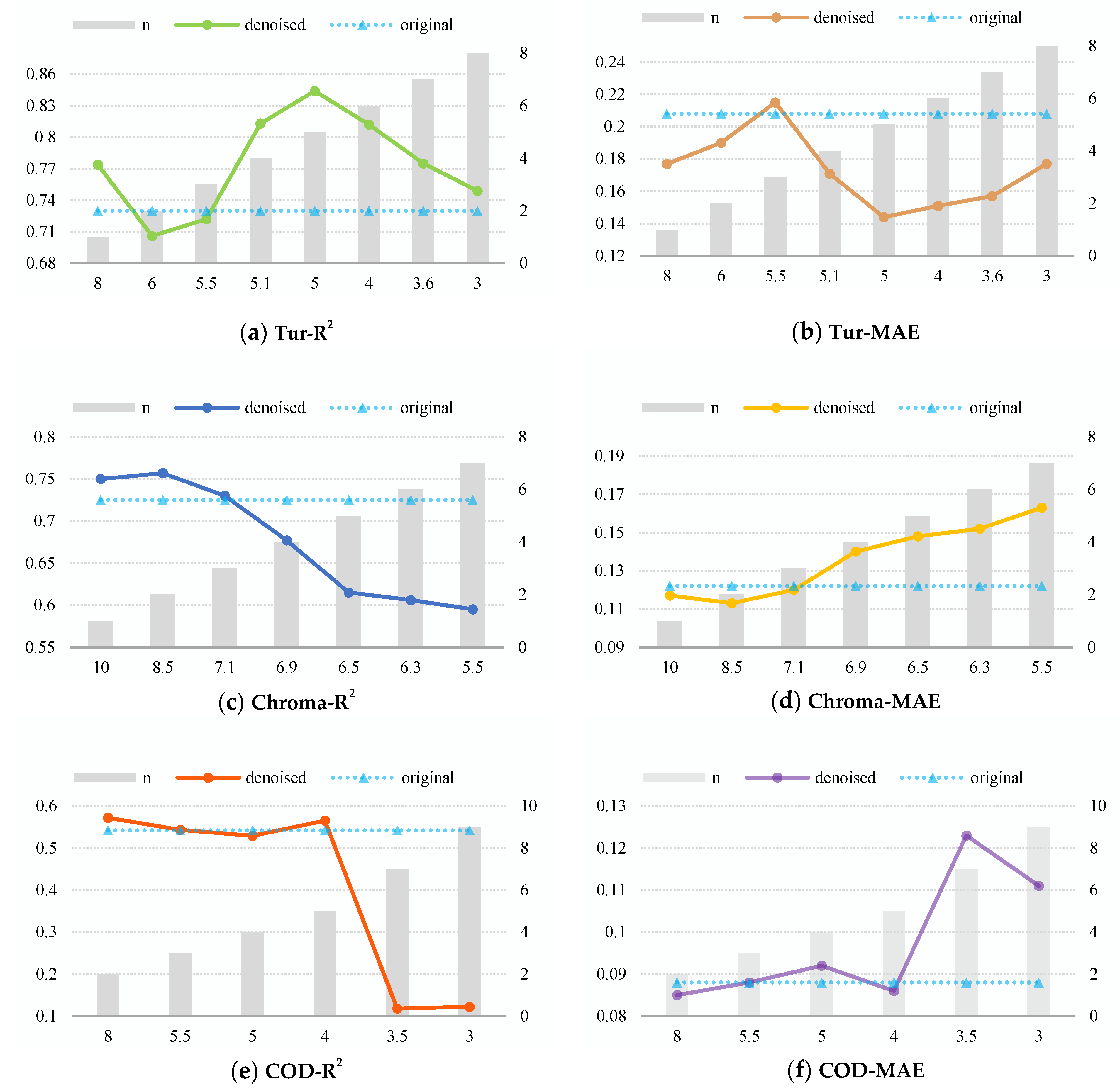
The value of parameter α is directly related to the number of labels that are judged to be noisy, thus affecting the model results. In order to study the influence of the value of parameter α on the performance of the model, we uniformly use the RFR method to conduct parameter adjustment experiments for three water quality parameters. In the experiment, we used the divided 28 samples for training model and eight samples for testing. The final results are shown in Figure 5. The horizontal axis represents the value of the parameter α, the vertical main axis represents the evaluation index such as R2 and MAE on testing data, and the vertical secondary axis represents the number of detected noisy instances n.
As shown in Figure 5a,b, in the experiment of retrieving turbidity, as the value of α gradually decreases, the number of instances n that are identified to be noisy labels gradually increases. When n goes from two to five, the model performance on the test set gets promoted, and when n continues to increase, the model performance starts to drop. We believe that when n is less than five, with the elimination of abnormal outliers, the model gradually learns the correct mapping. When n is greater than five, we cannot guarantee the fidelity of the data due to eliminating too many samples, and the model performance starts to degrade.
Figure 5c,d represents, respectively, the R2 and MAE results of the model on the test set in the chroma inversion experiment. It can be seen from the figure that when n is less than three, the model performance has a certain improvement. When n is greater than three, the model performance gradually degrades. We can conclude from the results that the noisy-label contamination of chroma is not as severe as that of turbidity, and when gradually starting to remove more outliers, the model fails to learn a complete mapping, resulting in performance decline.
Figure 5e,f represents the R2 and MAE results of the model on the test set in the COD inversion experiment, respectively. It can be seen from the figure that when n is less than four, the performance of the model decreases slowly, and when n is greater than four, the performance of the model on the test set degrades severely. We suppose that this is because the outliers in the COD data carry important feature information rather than polluted noise information. Model performance drops when outliers that carry important information are gradually removed.
4. Discussion
In this section, we want to discuss about three issues we met in the experiment. The first one is the invalid pixels in the experiment. The second issue is the suitable time for UAV imaging. The third one is the limitations of UAV considering meteorological conditions and practical operations.
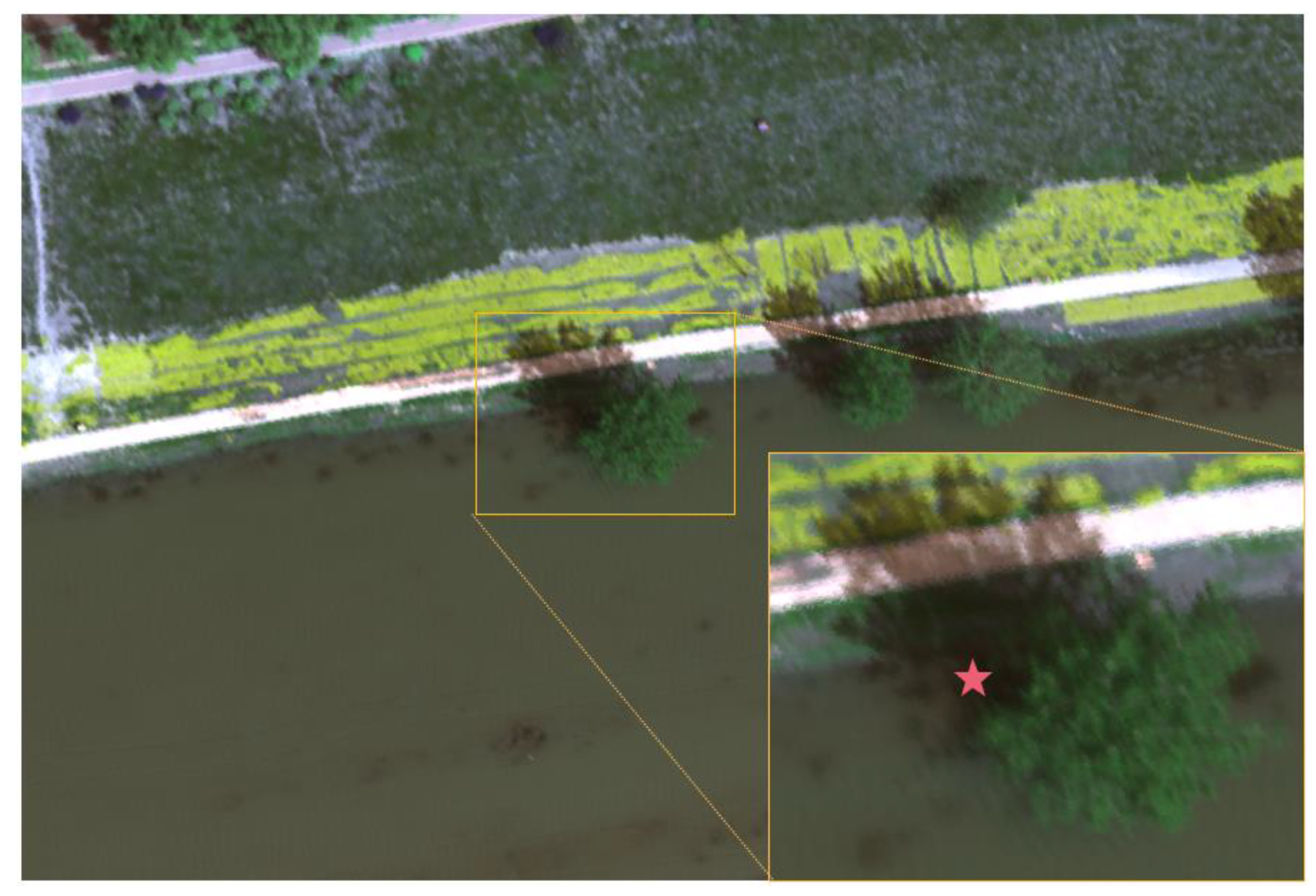
In Section 2.1.1, we introduce that 40 sampling points are arranged. However, four sampling points are removed because of shadow of trees. The invalid pixels in the experiment are presented in Figure 6. It is worth noting that when sampling, the shadow did not cover the site. When the UAV flew by, the shadow changed, and covered the sampling site. While sampling, the site may not be too close to trees or other tall buildings. Furthermore, in previous trial, the sunlight reflection will also affect the data quality.
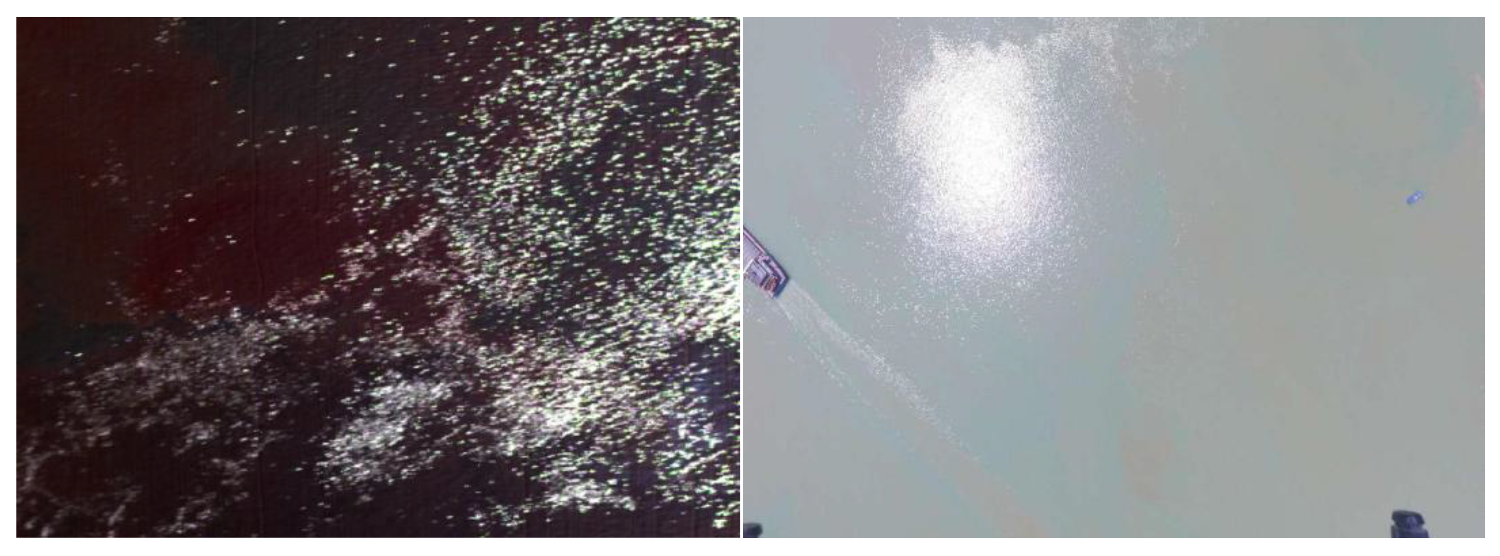
Suitable time for UAV imaging needs to be considered to avoid sunlight reflection. It is not suggested to fly UAV at noon, especially it is sunny, the sunlight may be perpendicular to the surface of water. The images obtained at noon is shown in Figure 7. The light is intense so image is over-exposed, useful information will be lost and the value of pixels reaches the maximum. Severe meteorological conditions such as strong winds and precipitation even make UAV unable to take off.
Another issue worth noting is battery. The UAV in the experiment is DJI Wind 4. The theoretical flying time is about 25 minutes. The maximum flying speed is 14 m/s. However, in practical, UAV ascends to specified altitude and lands on ground will consume 30 percent electricity. So, the actual time for UAV imaging is limited. This characteristic hinders the development of UAV based method to a wider range of detection.
5. Conclusions
In this study, a problem is raised that when using the existing UAV method to retrieve the flowing water body, the retrieving performance of water quality parameters such as turbidity and suspended solids changes quickly. As it is difficult to synchronize the time when collecting water quality data, it is easy to introduce label noise and affect the model performance. Based on this problem, this paper proposes an enhanced RegENN instance selection scheme which can more accurately detect noisy label instances and the scheme has better performance on turbidity and chromaticity data. This is because the value of turbidity and chromaticity changes more quickly in a flowing water body. At the same time, in order to further improve the model feature extraction and fitting performance, this paper combines 1DCNN and Self-Attention mechanism to build a deep neural network model, which achieves the best performance in chromaticity and turbidity inversion experiments. The values of testing R2 on turbidity and chromaticity are 0.904 and 0.877 respectively. Furthermore, we conduct a detailed experimental analysis of the value of the parameter α. The parameter α determines the number of samples which are judged to be label noise. The experimental results show that when the UAV water quality parameter inversion is performed on the flowing water body, the parameters such as turbidity and chromaticity need to be processed by noise labels. Our proposed enhanced RegENN method is proved to be effective on these two water quality parameters.
In the future work, we will conduct experiments on different water bodies to further verify the applicability of this method. At the same time, we will collect more water quality parameters to further analyze the measurement stability of other parameters.
Author Contributions
Conceptualization, Y.L., J.L. and T.Y.; methodology, Y.L. and J.L.; software, Y.L. and Y.Z.; validation, Y.L. and T.Y.; formal analysis, X.W.; investigation, S.S.; resources, H.L.; data curation, Y.L.; writing—original draft preparation, Y.L.; writing—review and editing, T.Y.; visualization, Y.L.; supervision, T.Y.; project administration, T.Y.; funding acquisition, T.Y. All authors have read and agreed to the published version of the manuscript.
Funding
This work was supported in part by the National Defense Science and Technology Innovation Special Zone Project under Grant 2020-XXX-014-01, in part by the Chinese Academy of Sciences Strategic Science and Technology Pilot Project A under Grant XDA23040101, and in part by the Shanxi provincial key R&D plan project under Grant 2019SF-254.
Data Availability Statement
Not applicable.
Acknowledgments
We appreciate Lin Zhang for water sample collection and Yu Zhang for chemical analysis.
Conflicts of Interest
The authors declare no conflict of interest.
References
- Cui, M.; Sun, Y.; Huang, C.; Li, M. Water turbidity retrieval based on uav hyperspectral remote sensing. Water 2022, 14, 128. [Google Scholar] [CrossRef]
- Ying, H.; Xia, K.; Huang, X.; Feng, H.; Yang, Y.; Du, X.; Huang, L. Evaluation of water quality based on UAV images and the IMP-MPP algorithm. Ecol. Inform. 2021, 61, 101239. [Google Scholar] [CrossRef]
- Liu, H.; Yu, T.; Hu, B.; Hou, X.; Zhang, Z.; Liu, X.; Liu, J.; Wang, X.; Zhong, J.; Tan, Z.; et al. UAV-Borne Hyperspectral Imaging Remote Sensing System Based on Acousto-Optic Tunable Filter for Water Quality Monitoring. Remote Sens. 2021, 13, 4069. [Google Scholar] [CrossRef]
- Zhang, Y.; Wu, L.; Deng, L.; Ouyang, B. Retrieval of water quality parameters from hyperspectral images using a hybrid feedback deep factorization machine model. Water Res. 2021, 204, 117618. [Google Scholar] [CrossRef]
- Lu, Q.; Si, W.; Wei, L.; Li, Z.; Xia, Z.; Ye, S.; Xia, Y. Retrieval of water quality from UAV-borne hyperspectralimagery: A comparative study of machine learning algorithms. Remote Sens. 2021, 13, 3928. [Google Scholar] [CrossRef]
- Xiao, Y.; Guo, Y.; Yin, G.; Zhang, X.; Shi, Y.; Hao, F.; Fu, Y. UAV Multispectral Image-Based Urban River Water Quality MonitoringUsing Stacked Ensemble Machine Learning Algorithms—A Case Study of the Zhanghe River, China. Remote Sens. 2022, 14, 3272. [Google Scholar] [CrossRef]
- Allam, M.; Khan, M.; Meng, Q. Retrieval of turbidity on a spatio-temporal scale using landsat 8 SR: A case study of the ramganga river in the ganges basin, india. Appl. Sci. 2020, 10, 3702. [Google Scholar] [CrossRef]
- Cheng, X.; Li, G.; Xu, J.; Zhao, B.; Zhao, D.; Xiao, X. Combined remote sensing retrieval of river turbidity based on chinese satellite data. J. Yangtze River Sci. Res. Inst. 2021, 38, 128–136. [Google Scholar]
- Myint, S.; Walker, N. Quantification of surface suspended sediments along a river dominated coast with NOAA AVHRR and SeaWiFS measurements: Louisiana, USA. Int. J. Remote Sens. 2002, 23, 3229–3249. [Google Scholar] [CrossRef]
- Haji, G.; Melesse, M.; Reddi, L. A comprehensive review on water quality parameters estimation using remote sensing techniques. Sensors 2016, 16, 1298. [Google Scholar]
- Shi, J.; Shen, Q.; Yao, Y.; Li, J.; Chen, F.; Wang, R.; Xu, W.; Gao, Z.; Wang, L.; Zhou, Y. Estimation of Chlorophyll-a Concentrations in Small Water Bodies: Comparison of Fused Gaofen-6 and Sentinel-2 Sensors. Remote Sens. 2022, 14, 229. [Google Scholar] [CrossRef]
- Sun, X.; Zhang, Y.; Shi, K.; Zhang, Y.; Li, N.; Wang, W.; Huang, X.; Qin, B. Monitoring water quality using proximal remote sensing technology. Sci. Total Environ. 2022, 803, 149805. [Google Scholar] [CrossRef]
- Zhang, M.; Wang, L.; Mu, C.; Huang, X. Water quality change and pollution source accounting of Licun River under long-term governance. Sci. Rep. 2022, 12, 2779. [Google Scholar] [CrossRef]
- Jacob, G.; Ehud, B. Training deep neural-networks using a noise adaptation layer. In Proceedings of the ICLR 2017, Toulon, France, 24–26 April 2017. [Google Scholar]
- Han, B.; Yao, J.; Gang, N.; Zhou, M.; Tsang, I.; Zhang, Y.; Sugiyama, M. Masking: A new perspective of noisy supervision. In Proceedings of the NeurIPS 2018, Montréal, QC, Canada, 3–8 December 2018; pp. 5839–5849. [Google Scholar]
- Chen, X.; Gupta, A. Webly Supervised Learning of Convolutional Networks. In Proceedings of the 2015 IEEE International Conference on Computer Vision (ICCV), Santiago, Chile, 7–13 December 2015; pp. 1431–1439. [Google Scholar]
- Kordos, M.; Biaka, S.; Blachnik, M. Instance selection in logical rule extraction for regression problems. In Artificial Intelligence and Soft Computing; Springer: Berlin/Heidelberg, Germany, 2013; pp. 167–175. [Google Scholar]
- Jiang, G.; Wang, W.; Qian, Y.; Liang, J. A unified sample selection framework for output noise filtering: An error-bound perspective. J. Mach. Learn. Res. 2021, 22, 1–66. [Google Scholar]
- Guillen, A.; Herrera, L.; Rubio, G.; Pomares, H.; Lendasse, A.; Rojas, I. New method for instance or prototype selection using mutual information in time series prediction. Neurocomputing 2010, 73, 2030–2038. [Google Scholar] [CrossRef]
- Shen, Y.; Sanghavi, S. Learning with bad training data via iterative trimmed loss minimization. In Proceedings of the 36th International Conference on Machine Learning, Long Beach, CA, USA, 10–15 June 2019; Volume 97, pp. 5739–5748. [Google Scholar]
- Tanno, R.; Saeedi, A.; Sankaranarayanan, S.; Alexander, D.; Silberman, N. Learning from noisy labels by regularized estimation of annotator confusion. In Proceedings of the 2019 IEEE/CVF Conference on Computer Vision and Pattern Recognition (CVPR), Long Beach, CA, USA, 15–20 June 2019; pp. 11236–11245. [Google Scholar]
- Li, J.; Socher, R.; Hoi, S. Dividemix: Learning with noisy labels as semi-supervised learning. arXiv 2020, arXiv:2002.07394. [Google Scholar]
- He, Y.; Xiao, S.; Nie, P.; Dong, T.; Qu, F.; Lin, L. Research on the optimum water content of detecting soil nitrogen using near infrared sensor. Sensors 2017, 17, 2045. [Google Scholar] [CrossRef]
- Tao, Q.; Lu, T.; Sheng, Y.; Li, L.; Lu, W.; Li, M. Machine learning aided design of perovskite oxide materials for photocatalytic water splitting. J. Energy Chem. 2021, 60, 351–359. [Google Scholar] [CrossRef]
- Goodfellow, I.; Bengio, Y.; Courville, A. Deep Learning; MIT press: Cambridge, MA, USA, 2016. [Google Scholar]
- Mohri, M.; Rostamizadeh, A.; Talwalkar, A. Foundations of Machine Learning; MIT Press: Cambridge, MA, USA, 2018. [Google Scholar]
- Yoav, F.; Robert, E. A decision-theoretic generalization of on-line learning and an application to boosting. J. Comput. Syst. Sci. 1997, 55, 119–139. [Google Scholar]
- Tao, W.; Li, C.; Song, R.; Cheng, J.; Liu, Y.; Wan, F.; Chen, X. EEG-based emotion recognition via channel-wise attention and self attention. IEEE Trans. Affect. Comput. 2020. [Google Scholar] [CrossRef]
- Xie, B.; Wu, X.; Zhang, S.; Zhao, S.; Li, M. Learning diverse features with part-level resolution for person re-identification. In Proceedings of the Chinese Conference on Pattern Recognition and Computer Vision (PRCV), Nanjing, China, 16–18 October 2020. [Google Scholar]
- Zhang, Y.; Wu, L.; Ren, H.; Liu, Y.; Zheng, Y.; Liu, Y.; Dong, J. Mapping water quality parameters in urban rivers from hyperspectral images using a new self-adapting selection of multiple artificial neural networks. Remote Sens. 2020, 12, 336. [Google Scholar] [CrossRef]
- Dona, C.; Chang, N.; Caselles, V.; Juan, M.; Camacho, A.; Delegido, J.; Benjamin, W. Integrated satellite data fusion and mining for monitoring lake water quality status of the Albufera de Valencia in Spain. J. Environ. Manag. 2015, 151, 416–426. [Google Scholar] [CrossRef]
- Michaelsen, M.; Meidow, J. Stochastic reasoning for structural pattern recognition: An example from image-based UAV navigation. Pattern Recognit. 2014, 8, 2732–2744. [Google Scholar] [CrossRef]
- Laliberte, A.; Goforth, M.; Steele, C.; Rango, A. Multispectral remote sensing from unmanned aircraft: Image processing workflows and applications for rangeland environments. Remote Sens. 2011, 3, 2529–2551. [Google Scholar] [CrossRef]
- Tang, J.; Tian, G.; Wang, X.; Wang, X.; Song, Q. The methods of water spectra measurement and analysis I: Above-water method. J. Remote Sens. 2004, 8, 37–44. [Google Scholar]
- Curtis, D. Estimation of the remote-sensing reflectance from above-surface measurements. Appl. Opt. 1999, 38, 7442–7455. [Google Scholar]
- Uta, H.; Karl, S.; Sigrid, R.; Hermann, K. Determination of robust spectral features for identification of urban surface materials in hyperspectral remote sensing data. Remote Sens. Environ. 2007, 111, 537–552. [Google Scholar]
- Vaiphasa, C. Consideration of smoothing techniques for hyperspectral remote sensing. ISPRS J. Photogramm. Remote Sens. 2006, 60, 91–99. [Google Scholar] [CrossRef]
- Vaswani, A.; Shazeer, N.; Parmar, N.; Uszkoreit, J.; Jones, L.; Gomez, A.; Kaiser, L.; Polosukhin, I. Attention is all you need. In Proceedings of the Advances in Neural Information Processing Systems 30 2017, Long Beach, CA, USA, 4–9 December 2017. [Google Scholar]
- Woo, S.; Park, J.; Lee, J.; Kweon, I. Cbam: Convolutional block attention module. In Proceedings of the European Conference on Computer Vision (ECCV) 2018, Munich, Germany, 1–8 September 2018; pp. 3–19. [Google Scholar]
- Hu, J.; Shen, L.; Sun, G. Squeeze-and-excitation networks. In Proceedings of the IEEE Conference on Computer Vision and Pattern Recognition 2018, Salt Lake City, UT, USA, 18–22 June 2018; pp. 7132–7141. [Google Scholar]
- Li, S.; Zhang, L.; Liu, H.; Hugo, A.; Zhai, L.; Zhuang, Y.; Lei, Q.; Hu, W.; Li, W.; Feng, Q.; et al. Evaluating the risk of phosphorus loss with a distributed watershed model featuring zero-order mobilization and first-order delivery. Sci. Total Environ. 2017, 609, 563–576. [Google Scholar] [CrossRef]
- Lerman, P. Fitting segmented regression models by grid search. J. R. Stat. Soc. Ser. C (Appl. Stat.) 1980, 29, 77–84. [Google Scholar] [CrossRef]
- Chen, Q.; Zhang, Y.; Hallikainen, M. Water quality monitoring using remote sensing in support of the EU water framework directive (WFD): A case study in the Gulf of Finland. Environ. Monit. Assess. 2007, 124, 157–166. [Google Scholar] [CrossRef] [PubMed]
Figure 1.
The specific location of the study area.

Figure 2.
The sampling points of two experiments along Xiao River combining with the COD inversion map on 11 April.
Figure 2.
The sampling points of two experiments along Xiao River combining with the COD inversion map on 11 April.

Figure 3.
The detailed route planning and the flight area of UAV in the experiment.

Figure 4.
The band correlation curves of the water quality parameters (Turbidity, Chromaticity, COD). (a–c) are original band correlation curves of the water quality parameters. (d–f) are band correlation curves after the process of noisy instance selection.
Figure 4.
The band correlation curves of the water quality parameters (Turbidity, Chromaticity, COD). (a–c) are original band correlation curves of the water quality parameters. (d–f) are band correlation curves after the process of noisy instance selection.

Figure 5.
The accuracy results of different parameter value. (a,b) represents the R2 and MAE of retrieving Tur. (c,d) represents R2 and MAE of retrieving Chroma. (e,f) represents R2 and MAE of retrieving COD.
Figure 5.
The accuracy results of different parameter value. (a,b) represents the R2 and MAE of retrieving Tur. (c,d) represents R2 and MAE of retrieving Chroma. (e,f) represents R2 and MAE of retrieving COD.

Figure 6.
The invalid sampling points because of shadow of trees.

Figure 7.
The images obtained at noon. The sunlight reflection is intense.


Table 1.
Detailed statistics of the data.
| Variable | Unit | Minimum | Maximum | Mean | Median |
|---|---|---|---|---|---|
| Chroma | Hazen | 32.07 | 69.67 | 50.68 | 52.53 |
| Tur | NTU | 3.37 | 12.52 | 6.58 | 5.96 |
| COD | mg/L | 2.22 | 9.49 | 6.37 | 6.15 |
Table 2.
The structure of our proposed 1DCNN for water quality parameter retrieving.
| Name | Patch Size | Stride | Channel | Padding | Output Size | Pooling/Stride | Channel Ratio |
|---|---|---|---|---|---|---|---|
| Conv1 | 3 | 1 | 8 | 1 | 8 × 75 | Max 2/2 | |
| Conv2 | 3 | 1 | 24 | 1 | 24 × 37 | Max 2/2 | |
| Attention1 | 24 × 37 | 8 | |||||
| Conv3 | 3 | 1 | 32 | 1 | 32 × 18 | Max 2/2 | |
| Attention2 | 32 × 18 | 8 | |||||
| Fc1 | 64 | ||||||
| Fc2 | 32 | ||||||
| Fc3 | 1 |
Table 3.
The range of parameter α for different regression models.
| Range | Chroma | Tur | COD |
|---|---|---|---|
| RFR | 5–12 | 2–9 | 5–12 |
| KNN | 10–25 | 2–20 | 10–30 |
| Adaboost | 5–15 | 2–7 | 10–25 |
| PLSR | 3–8 | 2–10 | 5–15 |
| 1DCNN | 3–10 | 1–8 | 5–20 |
Table 4.
The accuracy results of retrieving Turbidity.
| Turbidity | Index | rfr | knn | adaboost | 1dcnn | plsr |
|---|---|---|---|---|---|---|
| original | train r2 | 0.893 | 0.321 | 0.972 | 0.992 | 0.471 |
| test r2 | 0.73 | 0.335 | 0.842 | 0.873 | 0.689 | |
| train MAE | 0.102 | 0.258 | 0.055 | 0.001 | 0.252 | |
| test MAE | 0.208 | 0.222 | 0.13 | 0.114 | 0.213 | |
| train acc | 0.928 | 0.357 | 1 | 1 | 0.464 | |
| test acc | 0.75 | 0.5 | 0.75 | 0.75 | 0.5 | |
| denoised | train r2 | 0.922 | 0.461 | 0.983 | 0.997 | 0.696 |
| test r2 | 0.844 | 0.634 | 0.891 | 0.904 | 0.676 | |
| train MAE | 0.088 | 0.201 | 0.042 | 0.001 | 0.149 | |
| test MAE | 0.144 | 0.188 | 0.101 | 0.084 | 0.211 | |
| train acc | 0.869 | 0.578 | 1 | 1 | 0.71 | |
| test acc | 0.75 | 0.5 | 0.75 | 0.875 | 0.5 | |
| n | 5 | 8 | 5 | 5 | 7 | |
| α | 5 | 8.5 | 3.2 | 3.5 | 3.9 |
Table 5.
The accuracy results of retrieving chroma.
| Chroma | Index | rfr | knn | adaboost | 1dcnn | plsr |
|---|---|---|---|---|---|---|
| original | train r2 | 0.957 | 0.779 | 0.985 | 0.998 | 0.831 |
| test r2 | 0.725 | 0.71 | 0.714 | 0.834 | 0.749 | |
| train MAE | 0.029 | 0.062 | 0.015 | 0.001 | 0.053 | |
| test MAE | 0.122 | 0.131 | 0.127 | 0.096 | 0.132 | |
| train acc | 1 | 1 | 1 | 1 | 1 | |
| test acc | 0.875 | 0.875 | 0.875 | 1 | 0.75 | |
| denoised | train r2 | 0.954 | 0.853 | 0.989 | 0.998 | 0.941 |
| test r2 | 0.757 | 0.687 | 0.725 | 0.877 | 0.747 | |
| train MAE | 0.028 | 0.051 | 0.013 | 0.001 | 0.035 | |
| test MAE | 0.113 | 0.127 | 0.113 | 0.093 | 0.137 | |
| train acc | 1 | 1 | 1 | 1 | 1 | |
| test acc | 0.875 | 0.75 | 0.875 | 1 | 0.875 | |
| n | 2 | 3 | 1 | 2 | 3 | |
| α | 8.5 | 20 | 8 | 7.5 | 4 |
Table 6.
The accuracy results of retrieving COD.
| COD | Index | rfr | knn | adaboost | 1dcnn | plsr |
|---|---|---|---|---|---|---|
| original | train r2 | 0.847 | 0.243 | 0.964 | 0.997 | 0.634 |
| test r2 | 0.542 | 0.17 | 0.574 | 0.453 | 0.344 | |
| train MAE | 0.066 | 0.161 | 0.025 | 0.001 | 0.114 | |
| test MAE | 0.088 | 0.128 | 0.089 | 0.091 | 0.086 | |
| train acc | 0.964 | / | 1 | 1 | 0.892 | |
| test acc | 0.75 | / | 0.875 | 0.75 | 0.75 | |
| denoised | train r2 | 0.817 | / | 0.971 | 0.998 | 0.603 |
| test r2 | 0.572 | / | 0.662 | 0.518 | 0.143 | |
| train MAE | 0.043 | / | 0.023 | 0.001 | 0.08 | |
| test MAE | 0.088 | / | 0.078 | 0.071 | 0.141 | |
| train acc | 1 | / | 1 | 1 | 0.962 | |
| test acc | 0.875 | / | 1 | 0.75 | 0.75 | |
| n | 2 | / | 2 | 2 | 1 | |
| α | 8 | / | 15 | 15 | 5 |
Publisher’s Note: MDPI stays neutral with regard to jurisdictional claims in published maps and institutional affiliations. |
© 2022 by the authors. Licensee MDPI, Basel, Switzerland. This article is an open access article distributed under the terms and conditions of the Creative Commons Attribution (CC BY) license (https://creativecommons.org/licenses/by/4.0/).
Share and Cite
MDPI and ACS Style
Liu, Y.; Liu, J.; Zhao, Y.; Wang, X.; Song, S.; Liu, H.; Yu, T. Retrieving Water Quality Parameters from Noisy-Label Data Based on Instance Selection. Remote Sens. 2022, 14, 4742. https://doi.org/10.3390/rs14194742
AMA Style
Liu Y, Liu J, Zhao Y, Wang X, Song S, Liu H, Yu T. Retrieving Water Quality Parameters from Noisy-Label Data Based on Instance Selection. Remote Sensing. 2022; 14(19):4742. https://doi.org/10.3390/rs14194742
Chicago/Turabian StyleLiu, Yuyang, Jiacheng Liu, Yubo Zhao, Xueji Wang, Shuyao Song, Hong Liu, and Tao Yu. 2022. "Retrieving Water Quality Parameters from Noisy-Label Data Based on Instance Selection" Remote Sensing 14, no. 19: 4742. https://doi.org/10.3390/rs14194742
Note that from the first issue of 2016, this journal uses article numbers instead of page numbers. See further details here.