Application of Time-Domain Airborne Electromagnetic Method to the Study of Qingchengzi Ore Concentration Area in China

Abstract

Qingchengzi is an important polymetallic mineral concentration zone in China. However, long-term mining has led to the depletion of proven reserves in the Qingchengzi ore concentration zone. Therefore, it is necessary to carry out prospecting in the periphery of the existing ore bodies. Taking into account the complex surface conditions of the Qingchengzi mining area, we carried out an airborne time-domain electromagnetic survey in this region and obtained a high-precision underground resistivity model which covers the whole area. The quasi-3D inversion result shows a good agreement with the surface geological information. After analyzing the relationship between the underground geological structures and the resistivity model, we constructed a geological model with the distribution of the main strata, the rock masses and the faults. The reconstructed resistivity distribution of the entire region added new knowledge to understand the geology of the Qingchengzi survey area.

1. Introduction

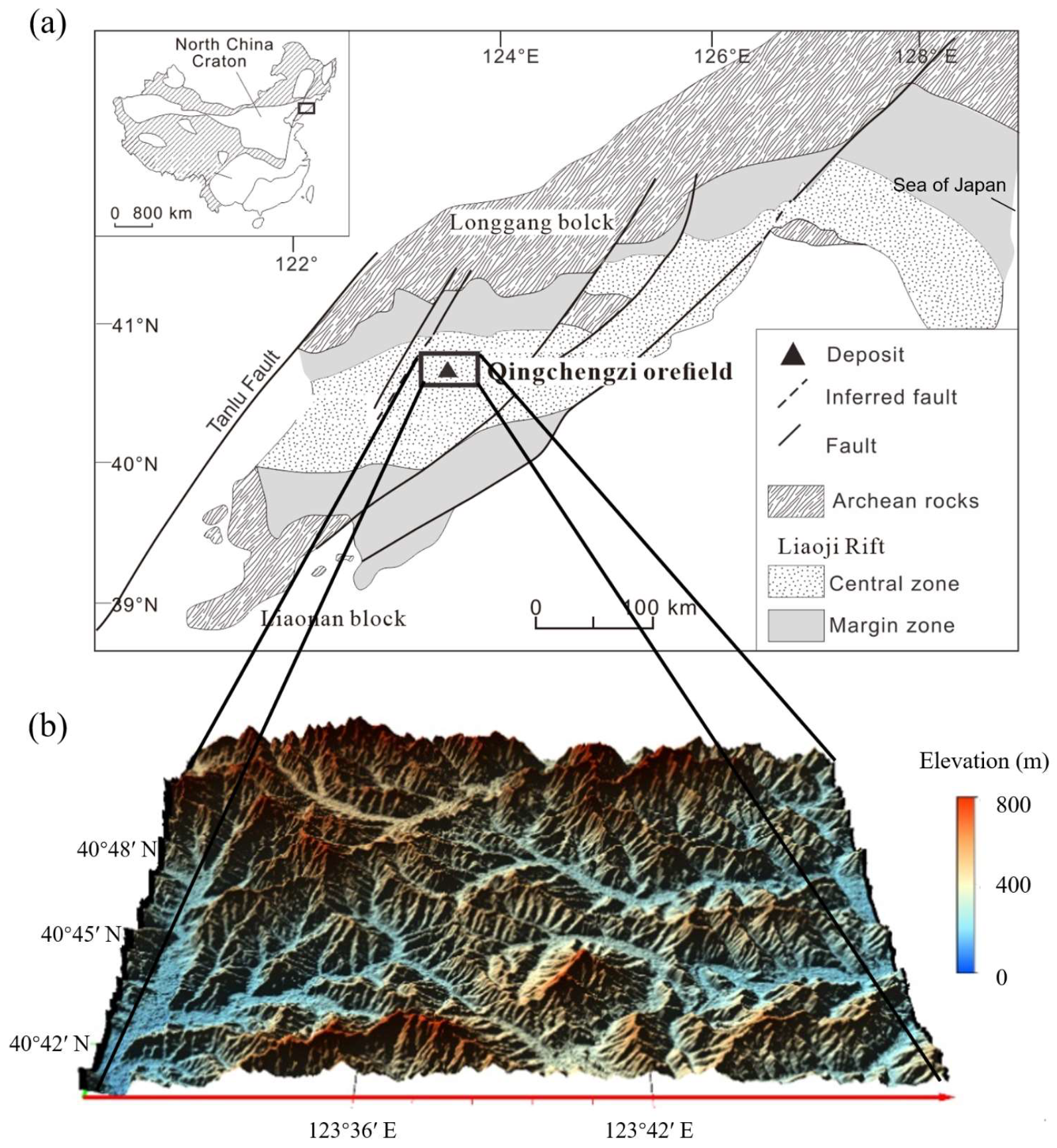
The Liaodong Peninsula is located in the Northeastern China Craton, which is the largest craton in China (Figure 1). There are three tectonic units in the Liaodong Peninsula: the Longgang block in the north, the Liaonan block in the south, while the Liaoji Rift is between them [1,2].

The Liaoji rift zone is an important metallogenic belt in China, and the Qingchengzi ore concentration area is located in the middle of Liaodong section of Liaoji Rift, with superior metallogenic geological conditions and multiple lead, zinc, gold, silver and other polymetallic deposits. The proven reserves have more than 1.6 million tons of lead-zinc deposit, more than 300 tons of gold, and more than 4000 tons of silver, and it is one of the most important polymetallic ore concentration areas in China.

The mining history of Qingchengzi ore field can be tracked back to the Ming dynasty (400 years ago). Due to the long mining history, the amount of mineral resources has decreased considerably. Qingchengzi and its adjacent areas are believed to have excellent potential for the discovery of additional mineralization. However, the mountain area covers more than 80% of this region, the forest coverage exceeds 70%, and the terrain conditions are very complex, resulting in inadequate geological research and geophysical prospecting.

Electromagnetic (EM) exploration methods are commonly used in mineral exploration [3,4,5,6]. The formation of minerals is closely related to the distribution of faults and magmatic activities. These fault and fracture zones are not only the migration channels of mineral resources, but also the storage space for the mineral resources. If there are other geological bodies or liquid intrusion in the fault or fracture zones, the resistivity could change significantly. Therefore, carrying out electromagnetic survey in the ore concentration area, obtaining high-resolution electrical characteristics of the subsurface, and identifying the distribution of faults can provide important information for the prospecting direction and the determination of the mineral target in this area.

EM exploration methods such as magnetotelluric (MT), audio magnetotelluric (AMT) and controlled-source audio magnetotelluric (CSAMT) have been widely used in mineral exploration in China [7,8,9]. All these methodologies are ground-based, and the working efficiency is greatly affected by the terrain conditions. Due to the large area and complex terrain conditions of the Qingchengzi ore field, it is difficult to carry out the conventional land exploration methods. Airborne electromagnetic (AEM) is a geophysical exploration technology that uses an aircraft platform to carry electromagnetic exploration equipment, which does not need ground personnel to approach the exploration area [10,11,12]. Therefore, AEM is suitable for the exploration work in the Qingchengzi area.

AEM technology originated in the 1950s, and its application fields include mineral, groundwater, oil and gas exploration, and environmental engineering [13,14,15,16,17,18,19,20,21,22]. The commonly used airborne electromagnetic systems are frequency-domain/time-domain fixed-wing systems and frequency-domain/time-domain helicopter systems [11,23]. In recent years, the helicopter time-domain (HTEM) system has been developed rapidly, including AeroTEM, Hoistem, HeliGEOTEM, SkyTEM and VTEM [24]. In the area of mineral exploration, the VTEM system has proven to be effective in characterizing the regional geologic or localized high conductivity signatures associated with deposits [25]. There are also studies on the detection capability of the VTEM systems. The Lalor copper-gold volcanogenic massive sulfide deposit region is an example where an EM anomaly known as South Bull’s Eye was well resolved although it is deeply buried [26]. In this study, the VTEM system was used for field data collection.

Data processing plays a vital role in the application of the HTEM method. The forward and inversion methods can be divided into one-dimension and multi-dimension. The 2D and 3D methods can provide more realistic electrical properties of the underground medium [27,28,29,30,31,32]. In order to speed up the computation and reduce the memory requirement, scientists have made unremitting efforts to develop a variety of accelerated computing technologies such as the moving footprint approach [33,34], the application of local meshes [35,36], the MUMPS (Multifrontal Massively Parallel Solver) and PARDISO (Parallel Direct Sparse Solver) direct solver technologies [37,38]. These methods have been successfully applied to many studies. However, challenges still exist in terms of the computational and memory requirements for large data.

Because the Qingchengzi HTEM survey generates a large amount of data comprised of hundreds of thousands of survey stations, 1D inversion is the first choice in this area. This inversion technique ensures fast computational speed that can handle a large amount of field data, and it has been widely used in HTEM data inversion [12,39,40]. The laterally constrained inversion (LCI) method proposed by Auken et al. [41,42] has its advantages in reducing non-uniqueness and recovering the lateral continuity of the inverted model compared with normal single site 1D inversion. The spatially constrained inversion (SCI) method was developed to further consider the model parameter constraints between different lines [43]. The LCI and SCI methods have been successful applied to many areas. For example, Kaminski et al. applied the SCI method to the VTEM data of a volcanogenic massive sulphide gold prospect, and the inversions result matched the known geology, adding new valuable information to the ongoing mineral exploration initiative [44]. Finn et al. inverted AEM data for Yellowstone National Park by using the LCI method, and obtained high-resolution resistivity models [45]. The LCI/SCI approach was chosen for this study.

In this work, we collected high-quality VTEM data along 2328 km lines, with a survey range of 456 square kilometers. The data was processed using the Workbench software [46]. The exploration results reveal the overall underground electrical characteristics of the ore concentration area, and the distribution of underground rock mass. Furthermore, main faults were inferred from the obtained model. The results of this study can provide important resistivity information to evaluate the underground structures and delineate the prospective mineral deposit area.

2. Geologic Settings

The Liaoji rift is a Paleoproterozoic rift developed on the basement of the Archean North China Craton. It has experienced several tectonic evolution processes such as crustal extension, mantle upwelling, magma intrusion and eruption, and volcanic activity weakening. A large volume of sedimentary strata was formed in the region, followed by crustal cracking and slow subsidence. A series of folds and faults were formed after the rift subsided and compressed. During these processes, the intruding magma provided the ore-forming materials while the folds and faults provided the ore-forming space.

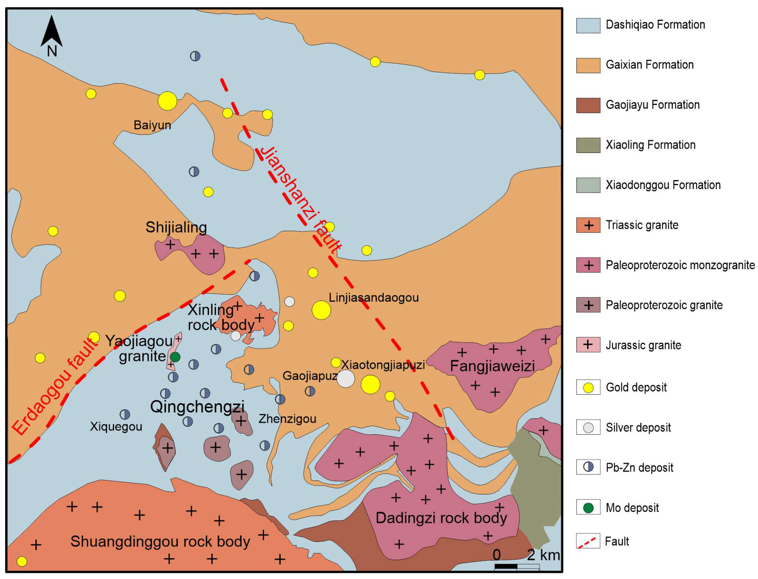
The main outcrops in the Qingchengzi ore concentration area are the Dashiqiao Formation, the Gaixian Formation and the Gojiayu Formation (Figure 2). The Dashiqiao Formation is the most widely distributed in this region, and has the main ore-bearing strata for lead-zinc deposits. It can be divided into three members: the first member (Pt₁d¹) is mainly composed of marble, diorite, diopside, granulite, schist and slate; the second member (Pt₁d²) includes schist, gneiss, sandstone, granulite, diorite and diopside; the third member (Pt₁d³) is widely exposed in the central and southern part of the survey area, and its lithology is mainly marble, schist, amphibolite and granulite. The Gaixian Formation is widely exposed and has the main ore-bearing strata for gold and silver deposits in this area. The first member of Gaixian Formation (Pt₁gx¹) is composed of schist, gneiss, granulite, diopside, and marble, while the second member (Pt₁gx²) is composed of schist, granulite, phyllite, sandstone, and a small amount of crystalline limestone. The Gaojiayu Formation is the smallest in volume, and it is distributed in the southern part of the survey area. The lithology is mainly composed of amphibolite schist, granulite, interbedded schist and marble.

The Qingchengzi ore concentration area has undergone an evolutionary process that led to the development of the Liaoji rift, and has also experienced the Indo-China and Yanshan tectonic magmatism. These tectonic activities have resulted in the formation of extremely developed fault structures. The structures of different periods are superimposed on each other, and the faults, which are of different nature and different directions, intersect each other. The existing geological information shows that there are mainly two groups of faults in this area, which run in the NW and NE directions. The main northwest-trending fault is the Jianshanzi fault, and the main northeast-trending fault is the Erdaogou fault. There are many other faults in the area, but their details are not clear. All these fault structures control the distribution of mineral deposits in the area.

The exposed granites in the Qingchengzi ore field were formed during the Palaeoproterozoic, Late Triassic, and Middle Jurassic magmatic events. The Paleoproterozoic monzogranites mainly include Dadingzi, Fangjiaweizi and Shijialing plutons, all of which have the same geology. The Late Triassic magmatism is represented by the Shuangdinggou and Xinling granite. The Middle Jurassic magmatism is represented by the Yaojiagou granite, which occurs as a small plug located in the southeast. In addition, a large number of vein rocks, such as lamprophyre, diabase, diorite, quartz porphyry and granite porphyry, are also developed in this area.

3. Data Acquisition, Processing and Inversion

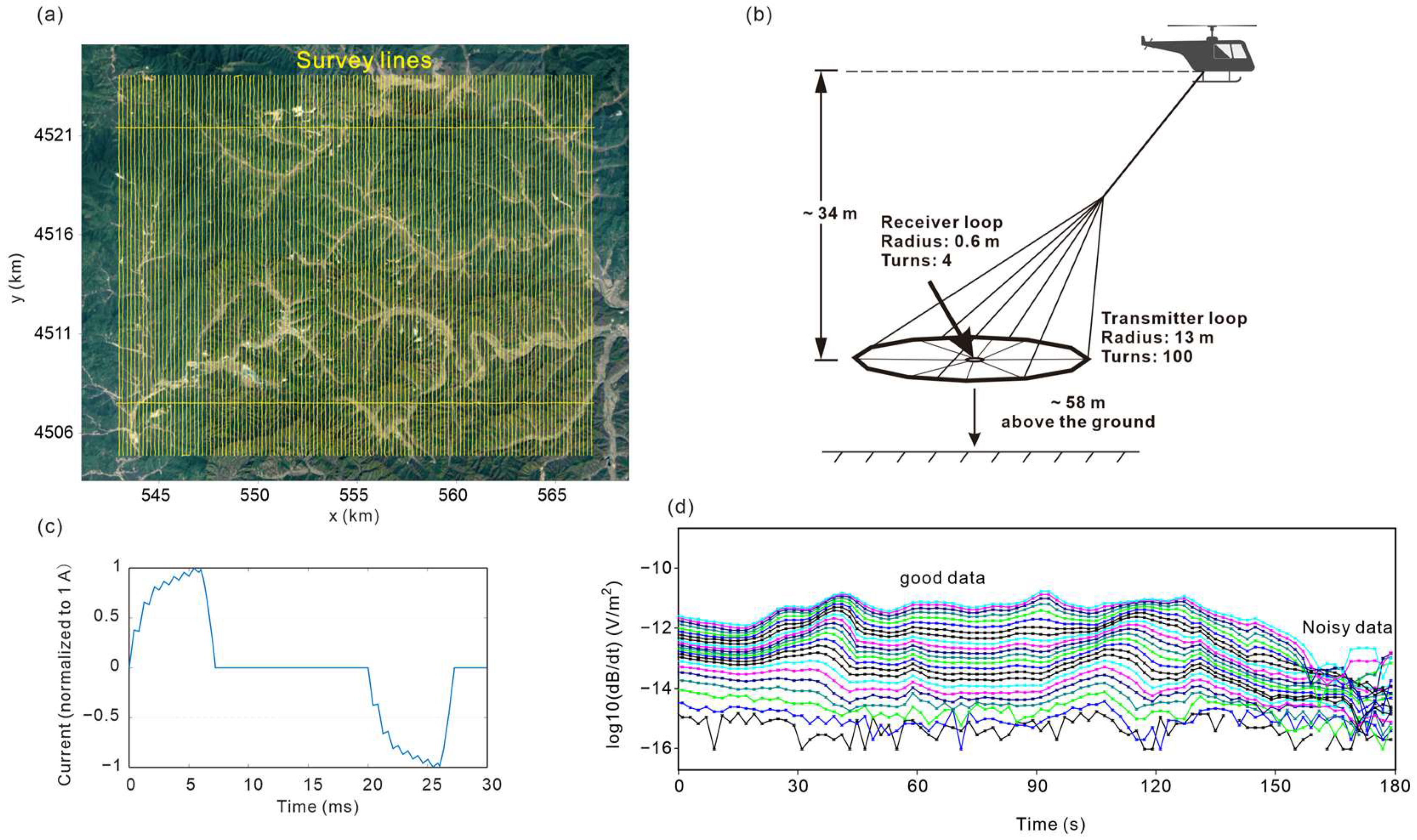
The airborne EM survey was conducted by Geotech Ltd. (Aurora, ON, Canada). The VTEM system was used to acquire the HTEM data along 120 NS trending survey lines and two EW tie lines in the Qingchengzi survey area, as shown by the yellow lines in Figure 3a. The length of each survey line in the NS direction is 19 km with a line spacing of 200 m, while the length of the EW survey lines is 24 km each. The total length of the survey lines is 2328 km.

From the observation, the average speed of the helicopter was 80 km/h and the average height of the coil above the ground was 58 m (Figure 3b). The peak dipole moment of the transmitting system was 400,000 NIA using a trapezoid shaped waveform with a 7.385 ms pulse width (Figure 3c). A total of 45 time-gates data were collected, ranging from 0.018 to 11.458 ms after the time off, and typical raw data are shown in Figure 3d.

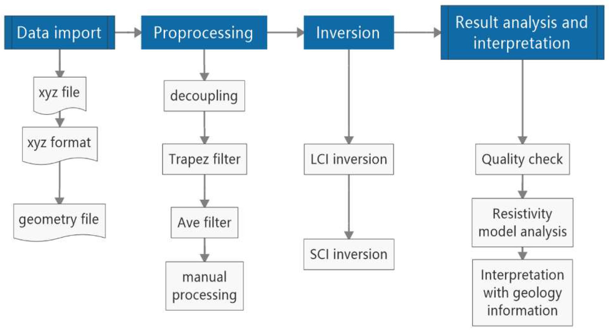
We used Aarhus Workbench to process the collected VTEM data in the survey area. The data processing of the VTEM data mainly includes four steps, as shown in Figure 4. Firstly, the raw data was transformed into a format that can be recognized by the Aarhus Workbench software. The second step includes the analysis of the field data, the suppression of data noise and the elimination of unqualified field data, etc. After completing this data preprocessing procedure, the inversion of all measurement data was completed to obtain the underground resistivity model of the entire survey area.

In the data preprocessing step, in order to reduce the demands of computing resources and improve the efficiency of data processing, the data were re-sampled to soundings at even time steps resulting in approximately one sounding per 20 m. The coupled data near villages and buildings were deleted before data averaging. Trapezoidal average windows were used to maintain the optimal resolution of the near-surface resistivity structures and a reasonable signal-to-noise ratio at late times. The average filter was also applied on the averaged data with the purpose of removing the remaining noisy data.

In the LCI and SCI inversion process, the resistivity and depth models are connected laterally or spatially by imposing similarity between the neighboring parameters, and all the soundings are inverted simultaneously to minimize a common objective function including lateral or spatial constraints [48].

The object function is expressed by

$$Q={\left(\frac{\delta d^T{C}_{obs}^{-1}\delta d+\delta r^T{C}_R^{-1}\delta r}{N_d+N_R}\right)}^{\frac{1}{2}},$$

(1)

where $C_{obs}^{}$ and $C_R^{}$ are the data and constraint covariance matrices; $\delta d$ represents the difference between the forward response and the observed data; $\delta r$ is the roughness of the model; $N_d$ and $N_R$ represent the number of data points and constraints.

During the inversion of the Qingchengzi field data, many individual flight lines were first inverted using the quasi-2D LCI approach. By doing this, we can test the influence of each inversion parameter on the data inversion results. Following this, we can analyze the reliability of the single line inversion results and find the optimized inversion parameter for the inversion of the entire dataset.

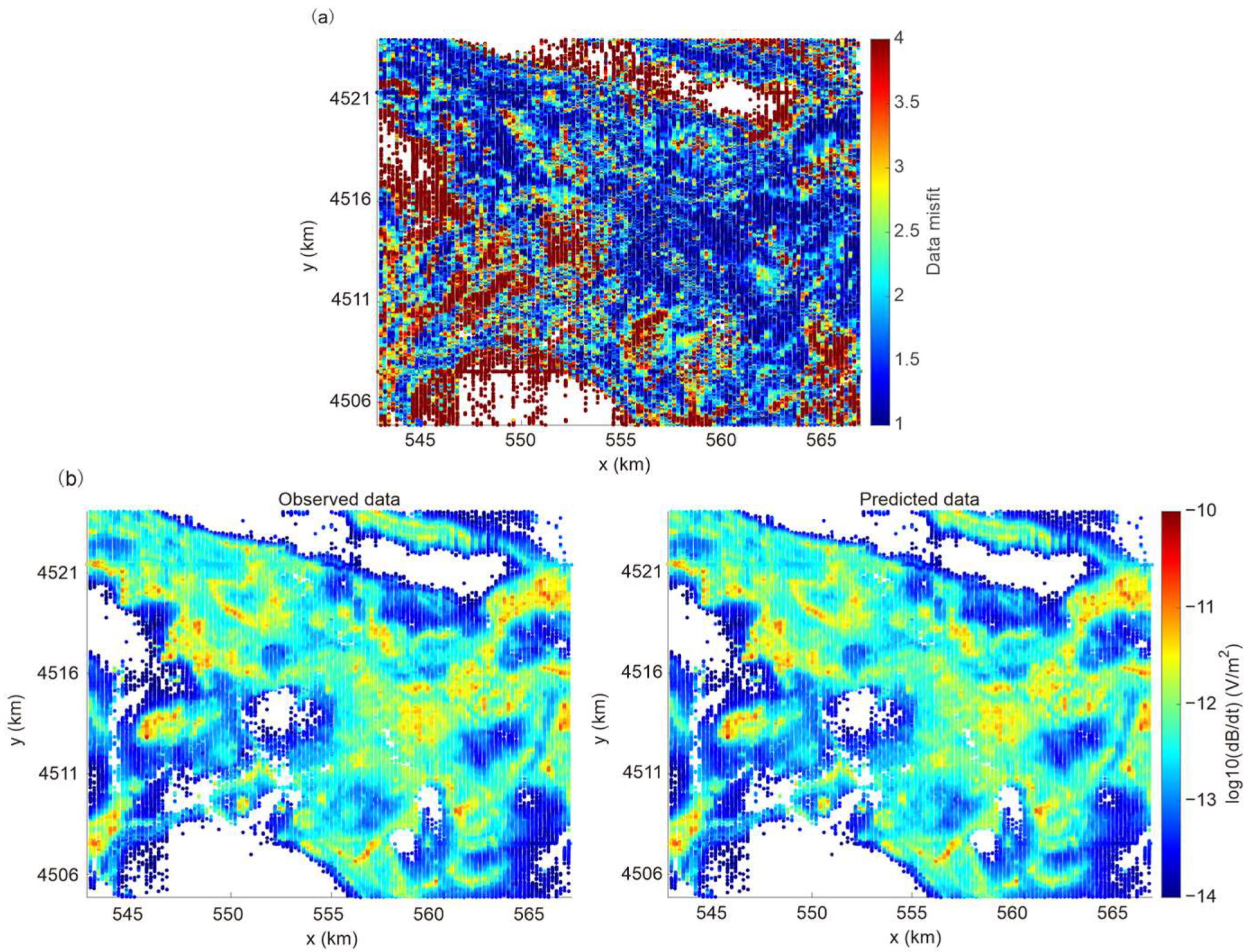
In the final SCI inversion, a uniform 30-layer starting model was found for each individual sounding using an adaption of Zohdy’s method [49]. The thickness of the layers in the model varied logarithmically, and the total thickness was 1000 m. The spatial constraints were set to a factor of 1.40, meaning that resistivities of adjacent soundings were allowed to change within roughly 40% from sounding to sounding. Moreover, the spatial constraints were set to decrease rapidly outside a radius of 20 m from each sounding. This constraint is considered loose; i.e., models can change rapidly with little adverse trade-off in the objective function. The full waveform including two pulses (Figure 3c) was accurately modelled [50], and the L2 norm was used to minimize the objective function. The root-mean-square data misfit for the survey area is shown in Figure 5a, and Figure 5b is a comparison between the observed and predicted data for one selected time.

4. Results and Discussions

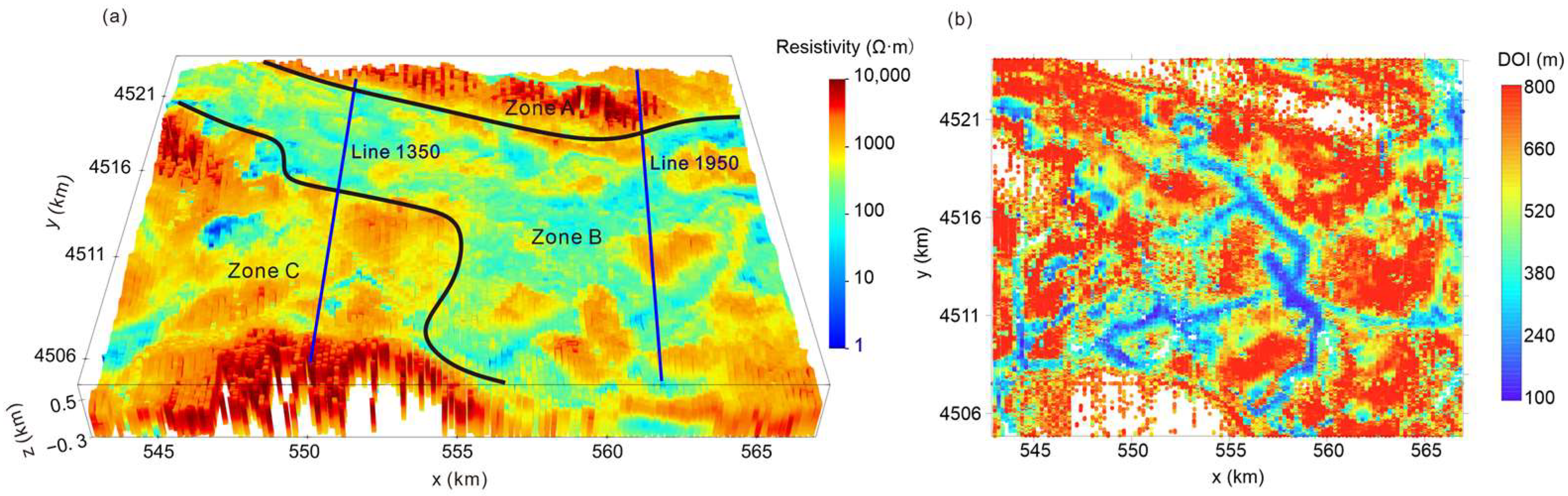
The final resistivity model obtained is shown in Figure 6a, from which we can get the resistivity distribution characteristics of the whole survey area. We also calculated the depth of investigation (DOI) for this inversion result (Figure 6b). The DOI estimation method proposed by Christiansen and Auken [51] was used, which is based on a recalculated sensitivity matrix of the final model. Although the DOI is highly model dependent and relies on a subjective threshold, this information can assist us in judging which parts of the model are data-driven and which parts are mainly driven by the starting model or the regularization of the inversion. The DOI (Figure 6b) trends to have a large value in the high resistivity region and a small value in the low resistivity region, which agrees well with the theory that the EM field attenuates slowly in the high resistivity medium and attenuates fast in the low resistivity medium.

From the overall resistivity distribution, the Qingchengzi ore field area can be roughly divided into three zones (Figure 6a). Zone A is located in the north of the ore concentration area, its resistivity changes from high (>3000 Ω·m) to low (<500 Ω·m) and then to medium (~1000 Ω·m) from the west to the east. Zone B is located in the middle, covering most of the survey area. The gold deposits are mainly distributed in this area. The overall resistivity of this zone is mainly less than 1000 Ω·m. Zone C covers the southwest of the survey area, and overall resistivity is high in this zone, where the Pb-Zn deposit is mainly distributed.

4.1. Relationship between Resistivity Model and Existing Geological Information

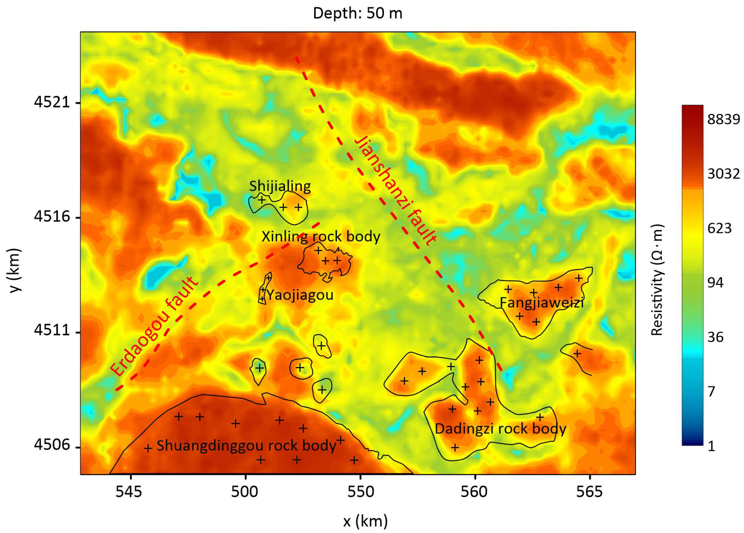
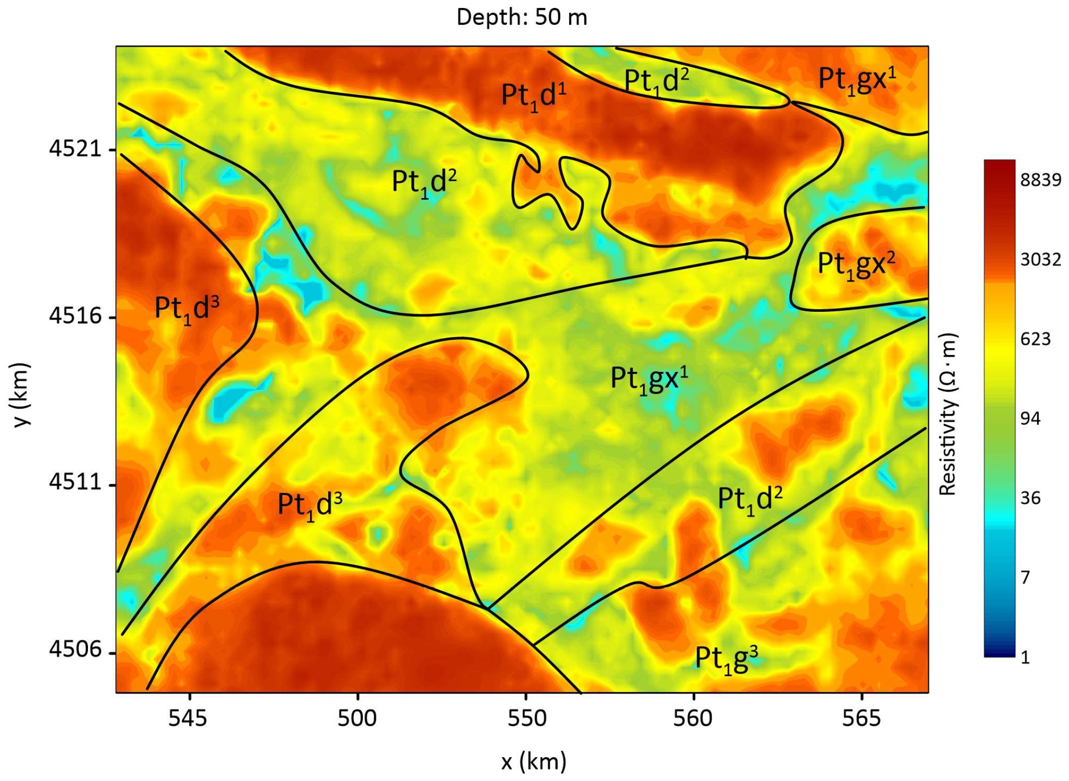
We compared the depth slice from the inverted resistivity model and the geological map (Figure 7). We can see that Dadingzi, Fangjiaweizi and Shijialing Paleoproterozoic monzogranite locations all show significantly high resistivity values, and the shape of the anomalous bodies are consistent with that of the rock mass. For the Triassic Shuangdinggou granite bodies, the depth slices also show high resistivity.

However, for the Xinling and Yaojiagou rock masses, the resistivity results do not indicate obvious anomalies. In addition, for the four small Proterozoic monzonitic granite bodies in the northern part of the Shuangdinggou Pluton, the depth slice indicates low-resistivity anomalies, which we infer were caused by the fragmentation of the rock mass.

The inverted model also shows the low resistivity characteristics of Jianshanzi and Erdaogou faults. The south end of the Jianshanzi fault is located at the edge of the Dadingzi high resistivity rock body, and the north end is located at the south edge of the NWW high resistivity rock body in the north of the survey area. The Erdaogou fault is located in the low resistivity band between the edges of different high resistivity bodies.

In order to further analyze the relationship between the electrical characteristics of the inversion model and the underground structure, two survey lines located in the east and west of the survey area (blue lines in Figure 6a) were selected for comparison with the available detailed geological information.

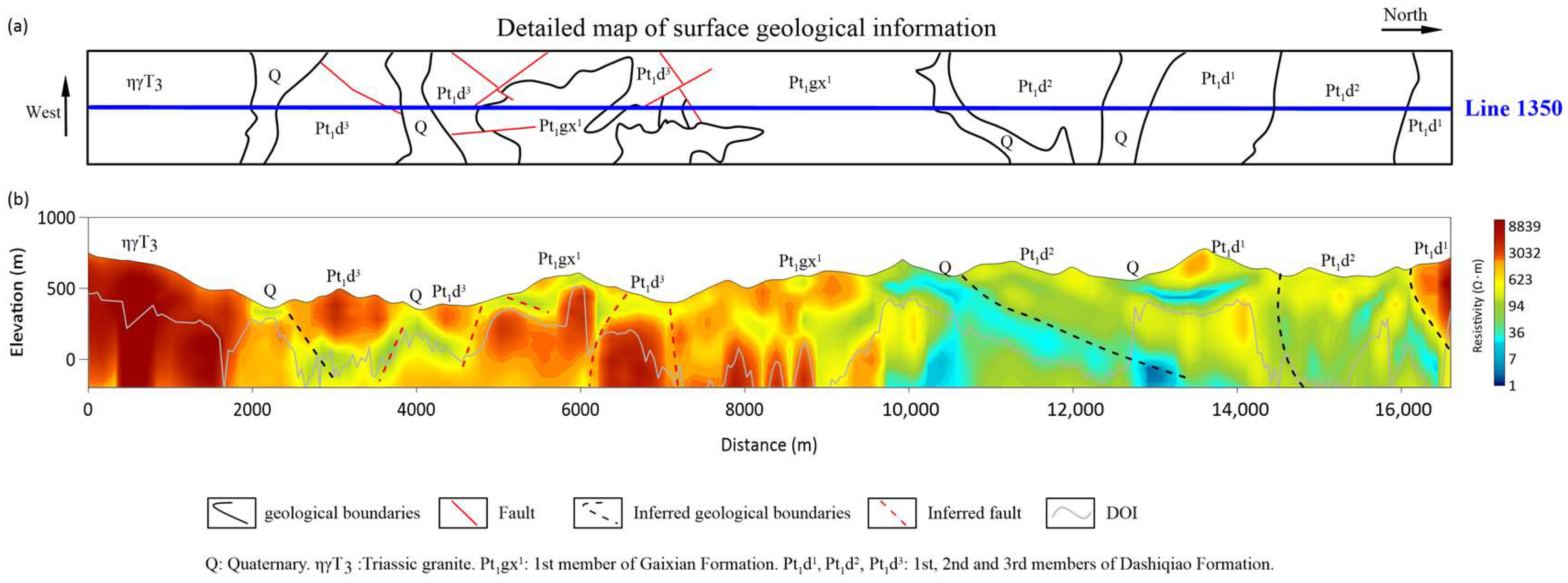
Figure 8 shows the comparison between the inversion profile of line 1350 and the available detailed geological information. The geological information shows that the Pt₁d³ and Pt₁gx¹ formations are mainly distributed in the southern part of the survey line, while the northern part of the survey line is mainly comprised of the Dashiqiao Formation (Pt₁d¹ and Pt₁d²). From the distance of 0 m to about 10 km, the subsurface resistivity is seen as medium-high (>1000 Ω·m), corresponding to the Pt₁d³ and Pt₁gx¹ formations. In the north from about 10 km, the Dashiqiao Formation shows different resistivity characteristics. The Pt₁d¹ formation in the north end of the survey line is characterized by high resistivity (~3000 Ω·m). In contrast, the Pt₁d² formation is characterized by low resistivity (~500 Ω·m).

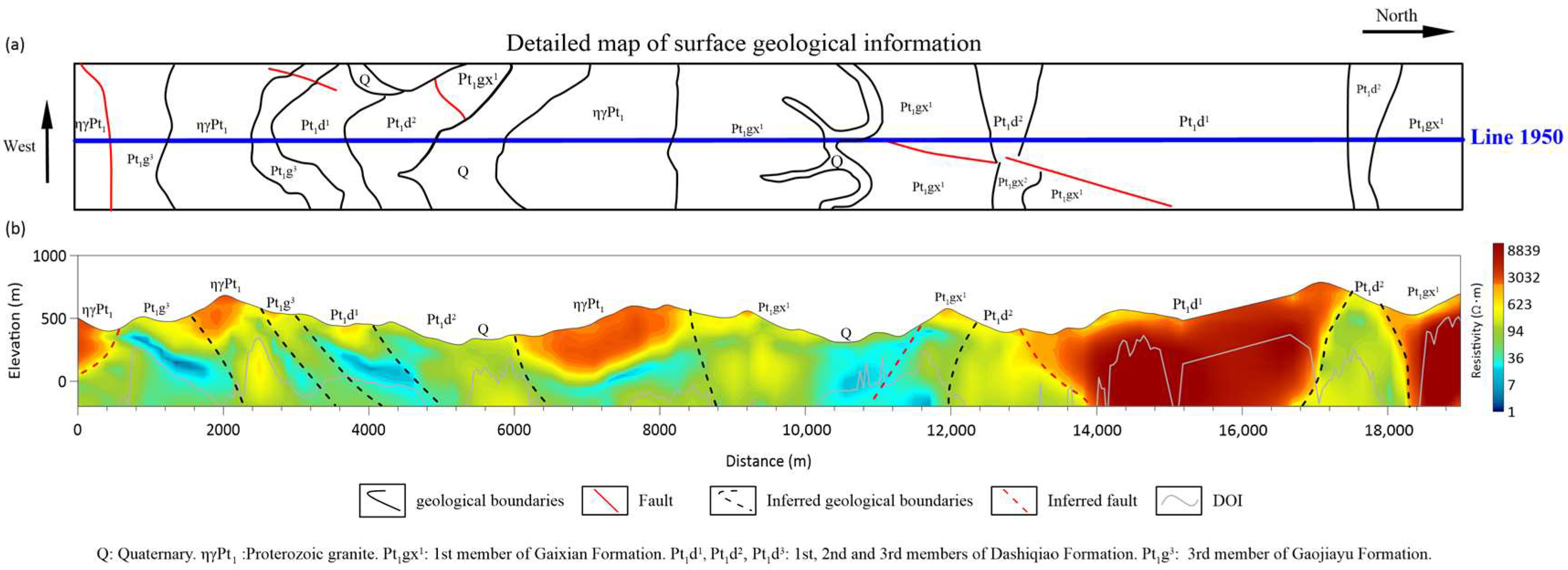
In line 1950 (Figure 9), the Dashiqiao Formation is mainly distributed between the distances of 12.5 km to 18 km. The resistivity of the Pt₁d¹ formation between 13 km to 17.5 km is the same as the one on the north end of line 1350, with high resistivity (>3000 Ω·m). Considering the distances of 12.5 km to 13 km and 17.5 km to 18 km, the resistivity of the Pt₁d² formation is also the same as those of line 1350, with a low resistivity value (~500 Ω·m). These show that there is a significant difference between the resistivity of the Pt₁d¹ and Pt₁d² formations. However, there are also a small number of Dashiqiao Formation strata between the distances of 3 km and 6 km and their resistivity difference is not the same as that in the north. In the southern part of the survey line, there is a small distribution of the Pt₁g³ formation, with medium-low resistivity values (<1000 Ω·m).

The Pt₁gx¹ formation is distributed in the middle (8.5 km to 12 km) and the north (>18 km) of the survey lines. The resistivity of the Gaixian Formation in the middle of the study area is low, which is lower than that of the formation in line 1350. Conversely, the Pt₁gx¹ formation in the north end is characterized by high resistivity (>3000 Ω·m), which is higher than the corresponding formation in line 1350. This is consistent with known geological information that these regions are in different sedimentary environments.

The rock mass location information in Figure 2 and the two detailed geological maps (Figure 8a and Figure 9a) are the same, but their formation distribution information is not consistent, especially at the boundary between the Gaixian Formation and Dashiqiao Formation in the north of line 1350. Based on the comparison between the resistivity characteristics and the different geological data, we believe that the geological information in Figure 8a and Figure 9a is reliable.

4.2. Geological Interpretation Based on the Resistivity Model

The resistivity characteristics of typical formations, fractures and rock masses in the survey area have been analyzed in the previous section. Now we would like to infer the underground geological model based on these analyses and the resistivity model.

The interpretation as the map of the different formations at the surface is shown in Figure 10. The NWW trending high resistivity bands in the north of the survey area distinguishes the boundaries of the Pt₁d¹ formation. On the other hand, the NWW trending low-resistivity band reflects the Pt₁d² formation. The medium-high resistivity area in the northeast of the survey area reflects the resistivity characteristics of the Pt₁gx¹ formation. In the west and south of the survey area, the medium-high resistivity values reflect the formation characteristics of the Pt₁gx¹ formation and the Pt₁d³ formation. The remaining large area with medium-low resistivity values trending mainly in the NW direction represents the strata of the Pt₁d² formation and the Pt₁gx¹ and Pt₁gx² formations. The Pt₁d² and Pt₁gx¹ formations have similar electrical characteristics, so their boundaries are mainly determined by the analysis of the detailed geology information of Lines 1350 and 1950. The Pt₁gx² formation is characterized by high resistivity compared with the surrounding Pt₁gx¹ formation, which is consistent with the known geological information. The small medium-low resistivity area in the southeast is inferred to be the location of the Pt₁g³ formation.

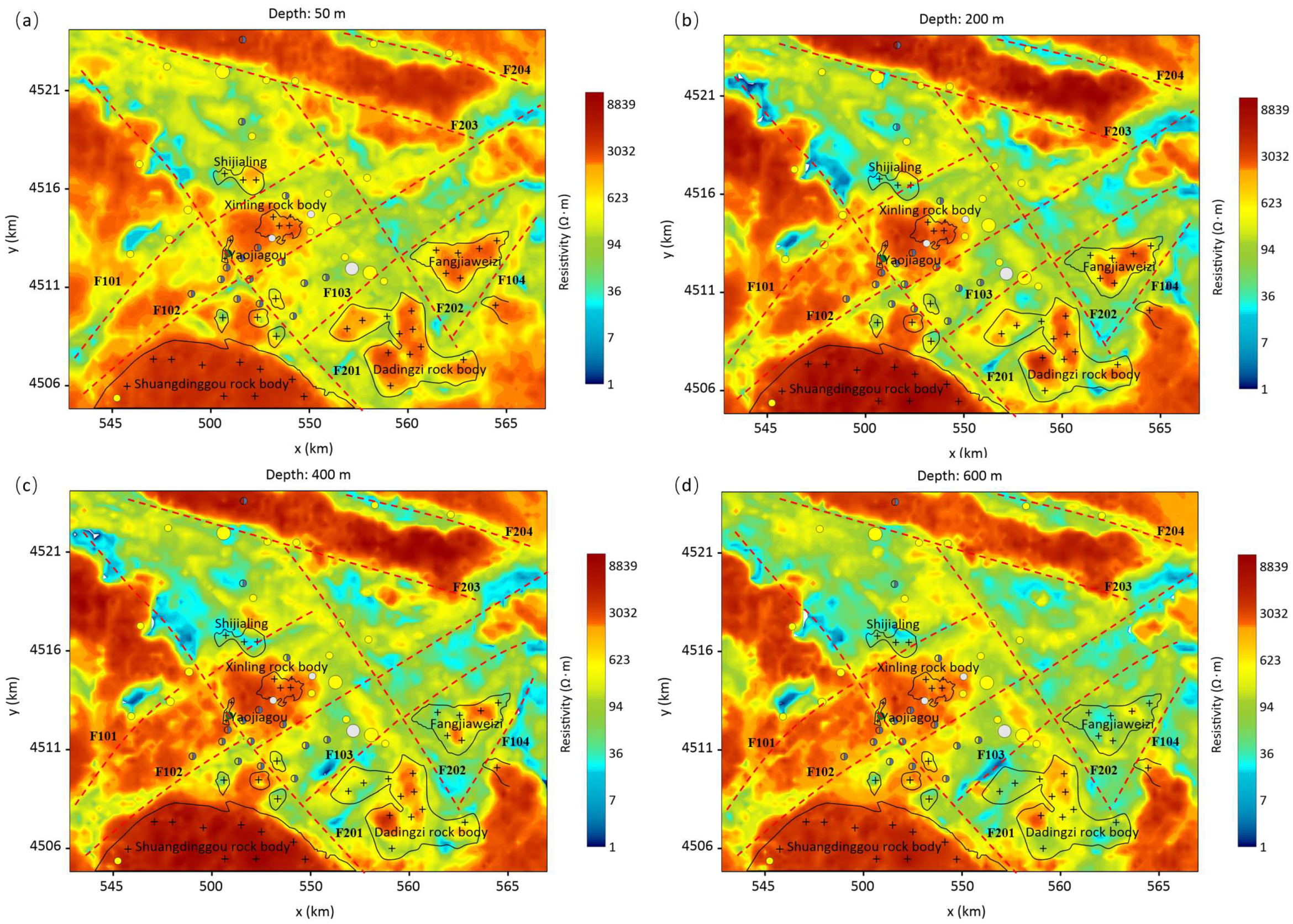
Faults play an important role in controlling the distribution of strata and rock masses, and they are closely related to mineralization. Therefore, it is of great significance to carry out fault structure interpretation for mineral exploration in this area. The faults are inferred based on the obtained earth resistivity distribution, as shown by the red dashed lines in Figure 11. The location of the F101 and the F202 faults are consistent with the known Erdaogou fault and Jianshanzi fault, respectively.

The inferred faults in the area can be divided into two groups of four with northeast and northwest trends. The F101 fault is distorted by F201 and cut off by F202. The F102 fault is distributed throughout the survey area and it is intercepted by the F201 and F202 faults. There are many lead-zinc deposits at the intersection of F102 and F201. Fault F103 is distributed in the south of the ore concentration area, intersecting with F201 and F202, respectively. Xiaotongjiapuzi gold deposit and Gaojiapuzi silver deposit are distributed at the intersection of the faults F103 and F202. The northeast side of the fault F201 is characterized by low resistivity and the southwest side is characterized by high resistivity. The fault F202 is inferred to have mainly controlled the development of Paleoproterozoic monzogranite. The faults F203 and F204 are located at the boundary between the high and low resistivity geological bodies, and are inferred to control the distribution of the Pt₁d¹ and Pt₁d² formations and the Pt₁gx¹ formation.

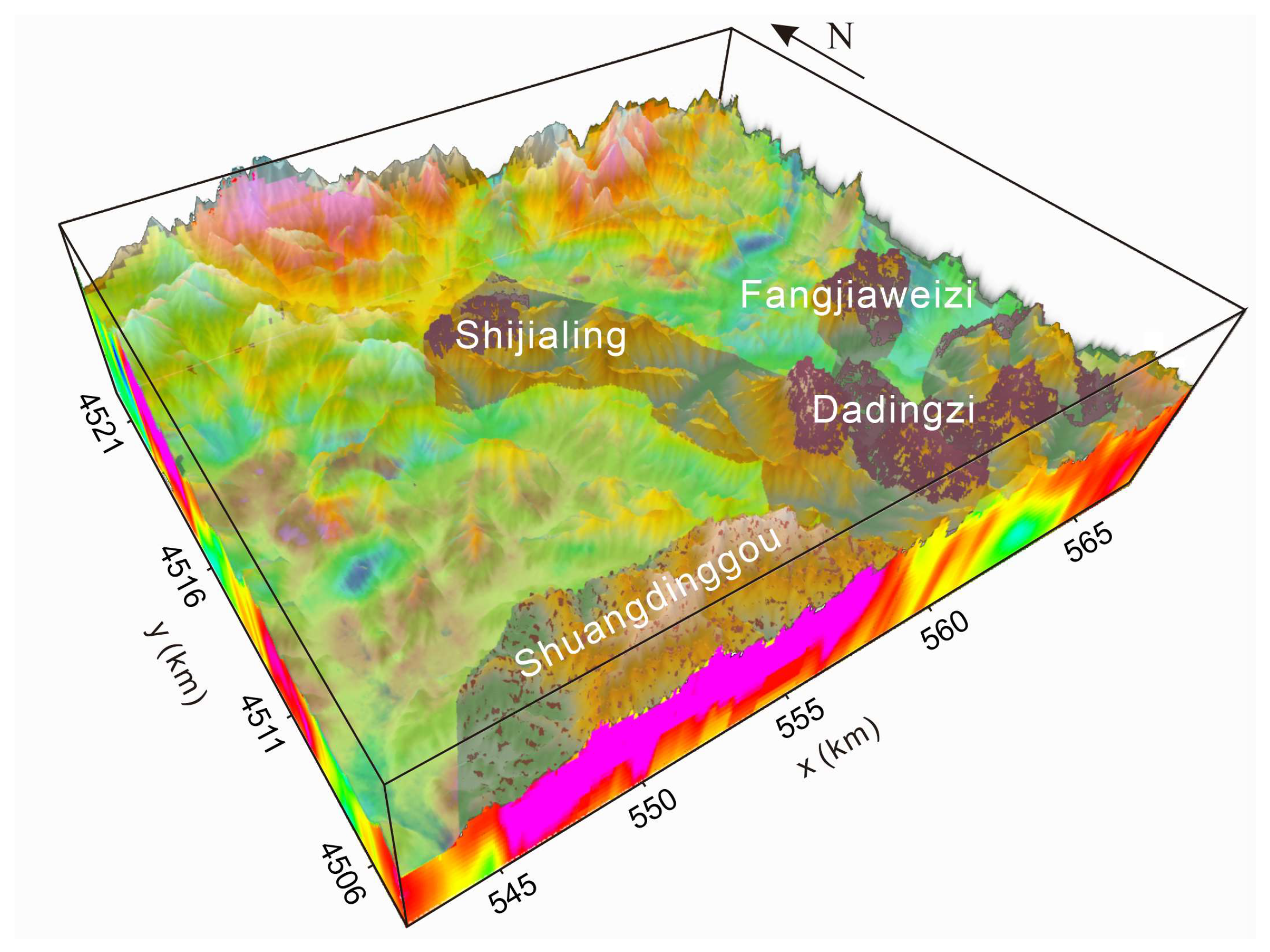
By comparing the resistivity results at different depths, we can also infer the variation in the underground lithology with depth. From the perspective of the subsurface resistivity distribution with depth (Figure 11a–d), the extent of the Dadingzi granite changes slightly, and its position gradually moves northward. Also, the Fangjiaweizi granite body has a shallow depth extent. As the depth increases, it extends toward the southwest and its lateral extent gradually decreases. Similarly, the Shijialing pluton has a quick northeastward transition at depth. The inversion result shows that the three rock bodies all show significantly high resistivity value, and they all tend to approach the location of the F202 fault at depth. It is speculated that the three rock bodies may be connected to each other at depth (Figure 12), and the Jianshanzi fault formation may have controlled the development of the migration pathway.

The shape and characteristics of the high resistivity anomaly at the location of the Shuangdinggou rock mass in the south of the survey area did not change much, indicating that the Shuangdinggou rock mass has little variation with depth, and the rock is intact. Conversely, no obvious high resistivity anomaly is observed over the location of the Xinling rock mass. Hence, it is speculated that rock alteration and fracture are strong in this area, which has led to no obvious resistivity difference between the rock mass and the surrounding rock.

We should note that all the above inferences are based on the resistivity model recovered by the smooth SCI approach, which uses an Occam-type regularization constraint and a 1D forward model. A smooth model will not be able to reproduce sharp geological layer boundaries, resulting in subjective boundary identification of anomalies. At the same time, the 1D approximation might be expected to fail to some unknown extent. When making geological interpretations, one should be aware of these risks.

5. Conclusions

The ore concentration area is not only an important production base for mineral resources, but also an important area for mineral resource exploration. Carrying out ore deposit prediction around known mineral deposits is an effective way to open up new areas for mineral prospecting. An excellent area for such study is the Qingchengzi gold concentration area which has considerable prospecting potential, but the complex terrain conditions have inhibited conventional electromagnetic surveys in this region. Therefore, this work presented the application of HTEM surveys in this area.

We obtained the resistivity characteristics of the whole survey area from the inverted resistivity model. The results show that there are obvious electrical resistivity differences between the Pt₁d¹ and Pt₁d² formations. The faults’ locations are generally characterized by low resistivity anomalies, and almost all the known deposits are located at the faults’ intersections and at the location where the high and low resistivity changes occur, not in the solid rock mass. The results also show that the granite bodies in the area generally have high resistivity value, and the Dadingzi, Fangjiaweizi and Shijialing rock bodies may be connected at depth. The results obtained in this paper can provide valuable complementary information for delineating concealed ore bodies in this area.

The geology structures in the Qingchengzi area are quite complex. The smooth regularization inversion technique used in this study provides vague pictures of sharp structures, which increases the risk when used for subsequent decision making such as selecting drilling targets. In order to get clearer and more reliable structures, the smooth solution in this study can serve as a starting model for sharp SCI inversion and the 3D inversion, which will be left to future research.

References

- Duan, X.; Zeng, Q.; Yang, J.; Liu, J.; Wang, Y.; Zhou, L. Geochronology, geochemistry and Hf isotope of Late Triassic magmatic rocks of Qingchengzi district in Liaodong peninsula, Northeast China. J. Asian Earth Sci. 2014, 91, 107–124. [Google Scholar] [CrossRef]
- Sun, G.; Zeng, Q.; Wang, Y.; Li, B.; Chen, P.; Santosh, M. Geochronology and geochemistry of Mesozoic dykes in the Qingchengzi ore field, Liaoning Province, China: Magmatic evolution and implications for ore genesis. Geol. J. 2019, 55, 5745–5763. [Google Scholar] [CrossRef]
- Smith, R. Electromagnetic Induction Methods in Mining Geophysics from 2008 to 2012. Surv. Geophys. 2014, 35, 123–156. [Google Scholar] [CrossRef]
- Upadhyay, A.; Singh, A.; Panda, K.P.; Sharma, S.P. Delineation of gold mineralization near Lawa village, North Singhbhum Mobile Belt, India, using electrical resistivity imaging, self-potential and very low frequency methods. J. Appl. Geophys. 2020, 172, 103902. [Google Scholar] [CrossRef]
- Vallee, M.A.; Smith, R.S.; Keating, P. Metalliferous mining geophysics—State of the art after a decade in the new millennium. Geophysics 2011, 76, W31–W50. [Google Scholar] [CrossRef]
- Zhdanov, M.S. Electromagnetic geophysics: Notes from the past and the road ahead. Geophysics 2010, 75, A49–A66. [Google Scholar] [CrossRef]
- Guo, Z.; Xue, G.; Liu, J.; Wu, X. Electromagnetic methods for mineral exploration in China: A review. Ore Geol. Rev. 2020, 118, 103357. [Google Scholar] [CrossRef]
- Hu, X.Y.; Peng, R.H.; Wu, G.J.; Wang, W.P.; Huo, G.P.; Han, B. Mineral Exploration using CSAMT data: Application to Longmen region metallogenic belt, Guangdong Province, China. Geophysics 2013, 78, B111–B119. [Google Scholar] [CrossRef]
- Farquharson, C.G.; Craven, J.A. Three-dimensional inversion of magnetotelluric data for mineral exploration: An example from the McArthur River uranium deposit, Saskatchewan, Canada. J. Appl. Geophys. 2009, 68, 450–458. [Google Scholar] [CrossRef]
- Auken, E.; Boesen, T.; Christiansen, A.V. A review of airborne electromagnetic methods with focus on geotechnical and hydrological applications from 2007 to 2017. Adv. Geophys. 2017, 58, 47–93. [Google Scholar]
- Yin, C.C.; Zhang, B.; Liu, Y.H.; Ren, X.Y.; Qi, Y.F.; Pei, Y.F.; Qiu, C.K.; Huang, X.; Huang, W.; Mia, J.J.; et al. Review on airborne EM technology and developments. Chin. J. Geophys.-Chin. 2015, 58, 2637–2653. [Google Scholar] [CrossRef]
- Yin, C.C.; Xiu-Yan, R.; Yun-He, L.; Yan-Fu, Q.; Chang-Kai, Q.; Jing, C. Review on airborne electromagnetic inverse theory and applications. Geophysics 2015, 80, W17–W31. [Google Scholar] [CrossRef]
- Chandra, S.; Choudhury, J.; Maurya, P.K.; Ahmed, S.; Auken, E.; Verma, S.K. Geological significance of delineating paleochannels with AEM. Explor. Geophys. 2020, 51, 74–83. [Google Scholar] [CrossRef]
- Di Massa, D.; Fedi, M.; Florio, G.; Vitale, A.; Viezzoli, A.; Kaminski, V. Joint interpretation of AEM and aeromagnetic data acquired over the Drybones kimberlite, NWT (Canada). J. Appl. Geophys. 2018, 158, 48–56. [Google Scholar] [CrossRef]
- Abedi, M.; Fournier, D.; Devriese, S.G.R.; Oldenburg, D.W. Integrated inversion of airborne geophysics over a structural geological unit: A case study for delineation of a porphyry copper zone in Iran. J. Appl. Geophys. 2018, 152, 188–202. [Google Scholar] [CrossRef]
- Paine, J.G.; Collins, E.W. Identifying Ground-water Resources and Intrabasinal Faults in the Hueco Bolson, West Texas, using Airborne Electromagnetic Induction and Magnetic-field Data. J. Environ. Eng. Geophys. 2017, 22, 63–81. [Google Scholar] [CrossRef]
- Siemon, B.; Costabel, S.; Voß, W.; Meyer, U.; Deus, N.; Elbracht, J.; Günther, T.; Wiederhold, H. Airborne and ground geophysical mapping of coastal clays in Eastern Friesland, Germany. Geophysics 2015, 80, WB21–WB34. [Google Scholar] [CrossRef]
- Legault, J.M.; Izarra, C.; Prikhodko, A.; Zhao, S.K.; Saadawi, E.M. Helicopter EM (ZTEM-VTEM) survey results over the Nuqrah copper-lead-zinc-gold SEDEX massive sulphide deposit in the Western Arabian Shield, Kingdom of Saudi Arabia. Explor. Geophys. 2015, 46, 36–48. [Google Scholar] [CrossRef]
- Yang, D.; Oldenburg, D.W. Three-dimensional inversion of airborne time-domain electromagnetic data with applications to a porphyry deposit. Geophysics 2012, 77, B23–B34. [Google Scholar] [CrossRef]
- Vrbancich, J. Airborne electromagnetic bathymetry and estimation of bedrock topography in Broken Bay, Australia. Geophysics 2012, 77, WB3–WB17. [Google Scholar] [CrossRef]
- Podgorski, J.E.; Auken, E.; Schamper, C.; Vest Christiansen, A.; Kalscheuer, T.; Green, A.G. Processing and inversion of commercial helicopter time-domain electromagnetic data for environmental assessments and geologic and hydrologic mapping. Geophysics 2013, 78, E149–E159. [Google Scholar] [CrossRef] [Green Version]
- Siemon, B.; Christiansen, A.V.; Auken, E. A review of helicopter-borne electromagnetic methods for groundwater exploration. Near Surf. Geophys. 2009, 7, 629–646. [Google Scholar] [CrossRef]
- Steuer, A.; Siemon, B.; Auken, E. A comparison of helicopter-borne electromagnetics in frequency- and time-domain at the Cuxhaven valley in Northern Germany. J. Appl. Geophys. 2009, 67, 194–205. [Google Scholar] [CrossRef]
- Christiansen, A.V.; Auken, E.; Viezzoli, A. Quantification of modeling errors in airborne TEM caused by inaccurate system description. Geophysics 2011, 76, F43–F52. [Google Scholar] [CrossRef]
- Witherly, K.; Irvine, R. The VTEM heli-time domain EM system-Four Case Studies. ASEG Ext. Abstr. 2006, 2006, 1–4. [Google Scholar] [CrossRef]
- Legault, J.M.; Plastow, G.; Zhao, S.K.; Bournas, N.; Prikhodko, A.; Orta, M. ZTEM and VTEM airborne EM and magnetic results over the Lalor copper-gold volcanogenic massive sulfide deposit region, near Snow Lake, Manitoba. Interpretation 2015, 3, Sl83–Sl94. [Google Scholar] [CrossRef]
- Cox, L.H.; Wilson, G.A.; Zhdanov, M.S. 3D inversion of airborne electromagnetic data. Geophysics 2012, 77, Wb59–Wb69. [Google Scholar] [CrossRef]
- Oldenburg, D.W.; Haber, E.; Shekhtman, R. Three dimensional inversion of multisource time domain electromagnetic data. Geophysics 2013, 78, E47–E57. [Google Scholar] [CrossRef]
- Liu, Y.H.; Yin, C.C.; Qiu, C.K.; Hui, Z.J.; Zhang, B.; Ren, X.Y.; Weng, A.H. 3-D inversion of transient EM data with topography using unstructured tetrahedral grids. Geophys. J. Int. 2019, 217, 301–318. [Google Scholar] [CrossRef]
- Qi, Y.; Li, X.; Yin, C.; Li, H.; Qi, Z.; Zhou, J.; Liu, Y.; Ren, X. 3-D Time-Domain Airborne EM Inversion for a Topographic Earth. IEEE Trans. Geosci. Remote Sens. 2020, 60, 1–13. [Google Scholar] [CrossRef]
- Zhang, B.; Yin, C.; Ren, X.; Liu, Y.; Qi, Y. Adaptive finite element for 3D time-domain airborne electromagnetic modeling based on hybrid posterior error estimation. Geophysics 2018, 83, WB71–WB79. [Google Scholar] [CrossRef]
- Ren, X.; Yin, C.; Macnae, J.; Liu, Y.; Zhang, B. 3D time-domain airborne electromagnetic inversion based on secondary field finite-volume method. Geophysics 2018, 83, E219–E228. [Google Scholar] [CrossRef]
- Cox, L.H.; Wilson, G.A.; Zhdanov, M.S. 3D inversion of airborne electromagnetic data using a moving footprint. Explor. Geophys. 2010, 41, 250–259. [Google Scholar] [CrossRef]
- Yin, C.C.; Huang, X.; Liu, Y.J.; Cai, J. Footprint for frequency-domain airborne electromagnetic systems. Geophysics 2014, 79, E243–E254. [Google Scholar] [CrossRef]
- Yang, D.K.; Oldenburg, D.W.; Haber, E. 3-D inversion of airborne electromagnetic data parallelized and accelerated by local mesh and adaptive soundings. Geophys. J. Int. 2014, 196, 1492–1507. [Google Scholar] [CrossRef]
- Haber, E.; Schwarzbach, C. Parallel inversion of large-scale airborne time-domain electromagnetic data with multiple OcTree meshes. Inverse Prob. 2014, 30, 055011. [Google Scholar] [CrossRef]
- Amestoy, P.R.; Duff, I.S.; L’Excellent, J.Y.; Koster, J. A fully asynchronous multifrontal solver using distributed dynamic scheduling. SIAM J. Matrix Anal. Appl. 2001, 23, 15–41. [Google Scholar] [CrossRef]
- Schenk, O.; Gartner, K.; Fichtner, W. Efficient sparse LU factorization with left-right looking strategy on shared memory multiprocessors. Bit 2000, 40, 158–176. [Google Scholar] [CrossRef]
- Constable, S.C.; Parker, R.L.; Constable, C.G. Occam’s inversion: A practical algorithm for generating smooth models from electromagnetic sounding data. Geophysics 1987, 52, 289–300. [Google Scholar] [CrossRef]
- Farquharson, C.G.; Oldenburg, D.W.; Routh, P.S. Simultaneous 1D inversion of loop-loop electromagnetic data for magnetic susceptibility and electrical conductivity. Geophysics 2003, 68, 1857–1869. [Google Scholar] [CrossRef]
- Auken, E.; Christiansen, A.V.; Jacobsen, B.H.; Foged, N.; Sorensen, K.I. Piecewise 1D laterally constrained inversion of resistivity data. Geophys. Prospect. 2005, 53, 497–506. [Google Scholar] [CrossRef]
- Auken, E.; Christiansen, A.V. Layered and laterally constrained 2D inversion of resistivity data. Geophysics 2004, 69, 752–761. [Google Scholar] [CrossRef]
- Viezzoli, A.; Christiansen, A.V.; Auken, E.; Sorensen, K. Quasi-3D modeling of airborne TEM data by spatially constrained inversion. Geophysics 2008, 73, F105–F113. [Google Scholar] [CrossRef]
- Kaminski, V.; Di Massa, D.; Viezzoli, A. Joint inversions of two VTEM surveys using quasi-3D TDEM and 3D magnetic inversion algorithms. Explor. Geophys. 2016, 47, 260–268. [Google Scholar] [CrossRef]
- Finn, C.A.; Bedrosian, P.A.; Holbrook, W.S.; Auken, E.; Bloss, B.R.; Crosbie, J. Geophysical imaging of the Yellowstone hydrothermal plumbing system. Nature 2022, 603, 643–647. [Google Scholar] [CrossRef]
- Auken, E.; Christiansen, A.V.; Westergaard, J.H.; Kirkegaard, C.; Foged, N.; Viezzoli, A. An integrated processing scheme for high-resolution airborne electromagnetic surveys, the SkyTEM system. Explor. Geophys. 2009, 40, 184–192. [Google Scholar] [CrossRef]
- Zeng, Q.D.; Chen, R.Y.; Yang, J.H.; Sun, G.T.; Yu, B.; Wang, Y.B.; Chen, P.W. The metallogenic characteristics and exploring ore potential of the gold deposits in eastern Liaoning Province. Acta Petrol. Sin. 2019, 35, 1939–1963. [Google Scholar] [CrossRef]
- Auken, E.; Christiansen, A.V.; Kirkegaard, C.; Fiandaca, G.; Schamper, C.; Behroozmand, A.A.; Binley, A.; Nielsen, E.; Effersø, F.; Christensen, N.B.; et al. An overview of a highly versatile forward and stable inverse algorithm for airborne, ground-based and borehole electromagnetic and electric data. Explor. Geophys. 2015, 46, 223–235. [Google Scholar] [CrossRef]
- Sattel, D. Inverting airborne electromagnetic (AEM) data with Zohdy’s method. Geophysics 2005, 70, G77–G85. [Google Scholar] [CrossRef]
- Fitterman, D.V.; Anderson, W.L. Effect of transmitter turn-off time on transient soundings. Geoexploration 1987, 24, 131–146. [Google Scholar] [CrossRef]
- Vest Christiansen, A.; Auken, E. A global measure for depth of investigation. Geophysics 2012, 77, WB171–WB177. [Google Scholar] [CrossRef]
Figure 1.
Regional geology of the study area. (a) Sketch map of the Liaoji rift zone and location of the Qingchengzi ore field. (b) Topographic map of Qingchengzi ore concentration area.
Figure 2.
Geological map of the Qingchengzi orefield (modified after Zeng et al. [47]).
Figure 3.
Data acquisition in Qingchengzi survey area. (a) Flight-line map over a satellite image. The yellow lines represent the position of the VTEM survey line, including 120 survey lines in the north-south direction and 2 survey lines in the east-west direction. (b) Configuration for ATEM method at Qingchengzi. (c) VTEM transmitter current waveform. (d) Typical VTEM raw data (plotted every two channels).
Figure 4.
The data processing flow for Qingchengzi VTEM data.
Figure 5.
Data misfit and comparison between the observed data and predicted data. (a) Data misfit. (b) A comparison between the observed data and predicted data at a time of 0.25 ms. The blank areas in the figures indicate the locations of the data that were removed during the preprocessing stage.
Figure 6.
The resistivity model and depth of investigation for this model. (a) The resistivity model obtained by SCI inversion. Due to the poor quality of the raw data or severe noise interference, there are some blank areas in the figure. The interpolated 50-m depth slice of the resistivity model is given in Figure 7. The whole survey area can be roughly divided into three regions: Zone A, Zone B and Zone C. The boundary of the three parts is shown in black curves. The two blue lines correspond to the cross-section locations shown in Figure 8 and Figure 9. (b) The depth of investigation for the resistivity model.
Figure 7.
Comparison between the 50-m depth slice of the resistivity model and the geological data in Figure 2 (the missing data of the inversion result are obtained by interpolation, which is also applied in the following figures).
Figure 8.
The detailed geological information near the line 1350 and the inversion profile result. (a) The detailed geological map near line 1350. The blue line represents the position of line 1350. (b) Resistivity section of line 1350.
Figure 9.
The detailed geological information near the line 1950 and the inversion profile result. (a) The detailed geological map near line 1950. The blue line represents the position of line 1950. (b) Resistivity section of line 1950.
Figure 10.
Main distribution of the different formations in the survey area inferred from resistivity model at a depth of 50 m.
Figure 11.
Resistivity slices at different depths, and the known surface rock mass geological data are projected onto the slices at each depth, as shown by black lines. The red dotted line is the fault or fracture inferred from the resistivity model. The northeast trending fault is named after the F1 prefix, and the northwestern fault is named after the F2 prefix. (a) Inversion result at 50 m. (b) Inversion result at 200 m. (c) Inversion result at 400 m. (d) Inversion result at 600 m.
Figure 12.
A basic understanding of the of underground rock masses inferred from the resistivity model.
Publisher’s Note: MDPI stays neutral with regard to jurisdictional claims in published maps and institutional affiliations. |
© 2022 by the authors. Licensee MDPI, Basel, Switzerland. This article is an open access article distributed under the terms and conditions of the Creative Commons Attribution (CC BY) license (https://creativecommons.org/licenses/by/4.0/).
Share and Cite
MDPI and ACS Style
Fu, C.; Di, Q.; Lei, D.; Wang, X.; Zhang, Y. Application of Time-Domain Airborne Electromagnetic Method to the Study of Qingchengzi Ore Concentration Area in China. Remote Sens. 2022, 14, 4716. https://doi.org/10.3390/rs14194716
AMA Style
Fu C, Di Q, Lei D, Wang X, Zhang Y. Application of Time-Domain Airborne Electromagnetic Method to the Study of Qingchengzi Ore Concentration Area in China. Remote Sensing. 2022; 14(19):4716. https://doi.org/10.3390/rs14194716
Chicago/Turabian StyleFu, Changmin, Qingyun Di, Da Lei, Xiaotian Wang, and Yilang Zhang. 2022. "Application of Time-Domain Airborne Electromagnetic Method to the Study of Qingchengzi Ore Concentration Area in China" Remote Sensing 14, no. 19: 4716. https://doi.org/10.3390/rs14194716
Note that from the first issue of 2016, this journal uses article numbers instead of page numbers. See further details here.