1. Introduction
In the last few years, large-scale and systematic information about the status and development of soils has moved into focus [
1,
2] because there is an increased demand for agricultural production [
3]. At the same time, soil erosion [
4] and soil-health degradation can be observed [
5]. Environmental covariates derived from Earth observation (EO) have already been used successfully for modelling soil information on a global [
6] and continental scale [
7]. Since the opening of the Landsat archives, the temporal compositing technique has become increasingly popular for many applications [
8,
9,
10,
11,
12]. Optical multispectral EO archives have been explored for detecting bare soils from temporal data stacks on a per-pixel basis. Then, the bare soil pixels are averaged to create soil reflectance composites (SRC). Thus, the temporary covering of mostly agricultural soils with vegetation in single data takes can be partially circumvented, resulting in enlarged bare soil areas in the reflectance composites. Example developments are presented by [
13] that have used the Landsat archive to derive a global map of bare ground gain by using 147 multitemporal metrics as input for tree-based regression and classification algorithms. The first operational SRC processors were developed by [
14,
15]. Ref. [
14] uses functionalities and data from the Google Earth Engine (Geospatial Soil Sensing System (GEOS3)). Ref. [
15] takes advantage of a processing environment and algorithms from the German Aerospace Center (DLR) for L2A processing (Soil Composite Mapping Processor—SCMAP). Both systems have been proven successful for agricultural areas at different spatial scales. Ref. [
16] presented a global study to explore the spectra of the bare Earth surface as input for soil resource monitoring. Ref. [
17] presented an exposed soil composite for the entire continent of Australia and tackled the challenge of applying a processor to very different biogeographical and climatic environments.
Several studies have created soil reflectance composites (SRC) and derived soil parameters such as soil organic matter (SOM) and clay content [
18,
19,
20], soil organic carbon content [
21,
22,
23,
24], calcium carbonates [
25] and other top-soil properties [
26]. The combination of sensors such as SAR and Sentinel-3 improves the bare SRC and retrievals [
19,
27,
28]. Refs. [
28,
29,
30] investigate expert-knowledge-based systems to select pixels with a minimal influence of disturbing factors such as crop residues, surface roughness and soil moisture.
The principles of almost all of the compositing techniques mentioned earlier are similar: (1) spectral reflectance indices are used to select bare soil pixels from the temporal data stack, (2) index thresholds are used to optimise the selection of undisturbed bare soil pixels and (3) the temporal length of the multitemporal data stack is defined. Based on previous scientific studies, temporal length definition depends on the used EO sensor and the application and the region of interest. It ranges between 1 year [
28], 2–4 years for Sentinel-2 [
20,
23,
27,
31] and 5 to more than 30 years for Landsat [
14,
15,
18,
25,
30]. In general, the temporal length of Landsat-based studies is larger due to its lower revisiting time of up to 16 days. In regions without measurable changes in top-soil organic matter contents, such as in Bavaria, Germany, larger time series such as 30 years of available Landsat datasets (1984–2014) can be used [
30,
32] with the advantage of covering the maximum amount of bare soils in the composite. However, by using such a long time series, the averaging of disturbing factors such as different soil moisture conditions, varying structural soil occurrences and remaining effects from non-photosynthetic active vegetation (NPV) is expected [
28]. These factors influence the quality of bare SRC [
14,
15] as well as the accuracy of the soil parameter retrievals [
28,
29]. Refs. [
33,
34] improved the underlying S2 Level 2A database by selecting dates after specific index thresholds, and [
23,
28] selected specific seasons to reduce disturbing effects, such as soil moisture as well as crop residues. Specifically, the “greening-up” period is promising since crop residues play a minor role. Ref. [
29] defined the “greening-up” time as the last date of acquisition where the soil is exposed before the crop develops and is mostly smoothed. However, this selection reduces the number of pixels available for composition, and an increase in temporal length across years might be necessary.
A wide range of strategies can be found in selecting the spectral index, and the threshold derivation technique. In a wide range of studies, the well-known normalised difference vegetation index (NDVI) is often used [
35] to separate the photosynthetically active areas (PV) from the non-active areas (NPV). Refs. [
13,
20] used an NDVI of <0.27, and [
14] used an NDVI of <0.25, followed by other spectral indices to account for the above-described disturbance factors. Ref. [
14] tested different empirically derived normalised burn ratio II (NBR2) thresholds (0.025–0.350) for a test area in Brazil using laboratory soil spectra. Ref. [
25] expanded this technique by using LUCAS top-soil spectral measurements to derive NDVI (
to 0.30) and NBR2 (
and 0.15) thresholds. Ref. [
31] uses empirically derived thresholds from NDVI (<0.20) and the bare soil index (BSI) of >0.08 for test areas in Italy. Ref. [
18] applied the BSI threshold (<0.021) that has been derived using airborne imaging spectrometer data from the Airborne Prism Experiment (APEX). Ref. [
19] combined NDVI and NBR2 and tested different index ranges by selecting the optimum threshold based on the best correlation between resampled LUCAS spectra and SRC spectra. Ref. [
15] developed a new index specifically for Landsat that combines the NDVI with a ratio of the near-infrared (NIR) and blue band to account for cloud artefacts that remain after cloud removal. The index thresholds have been derived using manually defined percentile measures. They have been proven stable across different years but not across different biogeographic regions in Germany. Thus, it has been found that percentiles are not transferable and strongly depend on the test site characteristics [
30]. This manual step should be avoided for operational processors to reduce human intervention during processing to a minimum.
Using thresholds for continental or even global scales requires robust and transferable rules for their definition. However, the rules defined in most of the studies mentioned above are not applicable at large (e.g., global) scales due to site-specific conditions. Only a few authors have used data-driven techniques such as regression trees [
13] and high-dimensional statistical methods [
17] for spectral compositing. Machine learning and artificial intelligence techniques sound promising but lack an independent training database that contains the variability of bare soil surfaces across the globe.
A more fundamental problem lies in the limited spectral information content of multispectral EO data (e.g., Sentinel-2) to discriminate between soil and spectrally similar surfaces such as urban areas and NPV. Such confusion (disturbance) can influence the modelling performance of soil parameter retrievals and, thus, are an essential research topic [
33,
36]. In this sense, index thresholds are just a compromise implying that a certain percentage of false positives needs to be minimised. On the other hand, it is a practical, easy-to-use and computationally efficient technique for large areas and massive data processing. By reviewing the literature mentioned above, we can conclude that there is currently no agreement in the community about the “best spectral index”. The fixed thresholds vary widely depending on the biogeographic zone and the climatic condition of the test area. The exclusion of urban areas is not critical since profound databases such as the Global Urban Footprint [
37], World Settlement Footprint [
11] and the Global Human Settlement Layer [
38] exist and are updated regularly to mask urban areas out. However, more significant problems are caused by NPV. These surfaces can only be distinguished from soils by using data resolving the narrow spectral absorption features at, e.g., 1.7 and 2.1 µm that characterise the cellulose and lignin content. Good experiences have been had with the NBR2 that is often used to account for the soil-NPV confusion, although it can only minimise the influence of spectrally similar surfaces. However, the definition of a transferable threshold remains a difficult task and has been solved differently by authors.
More insights are needed about the diversity of index thresholds across large areas and their impact on the resulting SRCs. For this purpose, there is a need for a more generic solution to derive thresholds for large-scale processing. The solution shall (1) be generally applicable, (2) allow for regionalised threshold derivation, (3) account especially for spectral similarities between bare soil and NPV and (4) be independent of specific spectral index selections.
This study aims to develop a generic methodology for deriving spectral index thresholds used to derive SRCs. For this purpose, the two most commonly used indices represented in the soil-related literature are selected: NDVI and NBR2. Further, a new index called PV+IR2 is developed that combines the information from the visible to near-infrared (VNIR) and the short-wave infrared (SWIR) wavelength region. Several technical objectives have to be attained: (1) a fully automatised threshold derivation technique to process large and diverse areas by objective means, (2) the evaluation of the three above-mentioned spectral indices to detect bare soils and to exclude pixels covering NPV and (3) the development of statistical measures to evaluate and compare the performance of SRC, including novel data products to assess the spectral uncertainty of the SRC.
This study gives more insights into the impact of selected indices and thresholds on resulting SRCs, which could influence the subsequent modelling of soil parameters. Moreover, it introduces measures and novel image products to evaluate the performance of SRCs as a database for the modelling part.
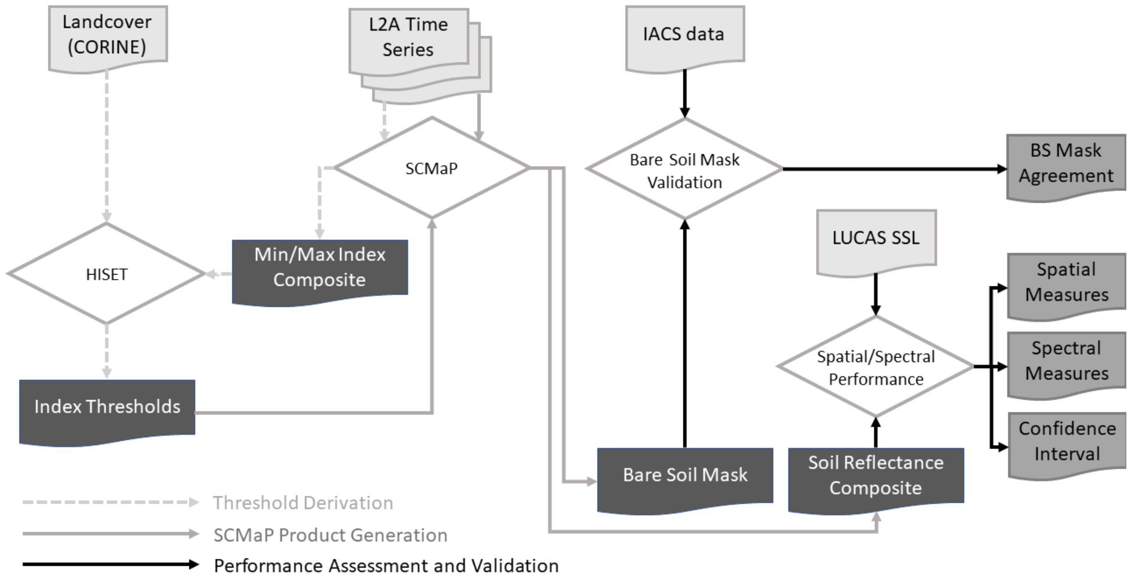
2. Materials and Methods
The analyses in this study are focused on part of Germany (
Section 2.1). For the Sentinel-2 tiles covering this area (
Section 2.2) and specific landcover types
Section 2.3), the spectral index thresholds are derived using the SCMaP (
Section 2.6) and the novel HIstogram SEparation Threshold (HISET) methods (
Section 2.7). Based on the set of thresholds, SCMaP is used again to generate six different SRCs that are compared within a performance assessment and validation step (
Section 2.8). For this purpose, the LUCAS Soil Spectral Library (SSL) (
Section 2.4) and the agricultural information from the
Integrated Administration and Control System (IACS) (
Section 2.5) are used to derive several spatial and spectral information products describing the performance and accuracy of the derived SRCs. An overview of the main analyses carried out in this study is given in
Figure 1.
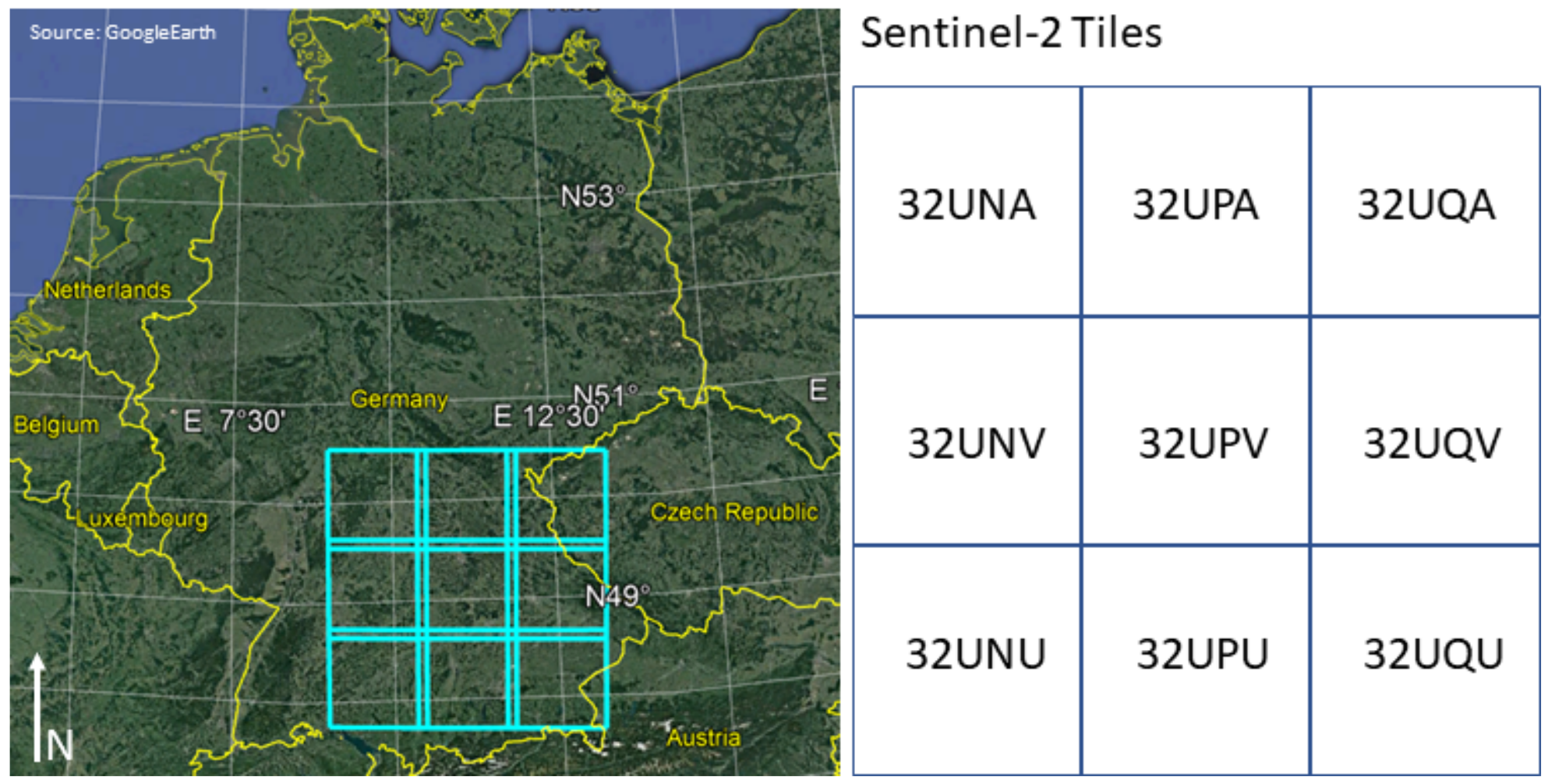
2.1. Test Area
All processing and analysis are performed for a mid-European test site covering large parts of the German federal state of Bavaria, Western parts of the Czech Republic and parts of Austria (
Figure 2).
The area of 108.504 km
2 is framed by larger forested areas such as the hilly Spessart in the Northwest, the Thuringian forest in the North and the Bavarian Forest and Sumava National Park in the East. The Southern half of the test site is dominated by several river systems such as the Danube, Lech, Iller, Isar and Inn. Especially in the South, several old peat bog areas, such as the Donaumoos, are mainly used for agricultural purposes. Based on the World Reference Base (IUSS Working Group WRB, 2015) classification, the dominating soil types of the test site are Cambisols and Luvisols [
6,
39], with SOC values ranging from 0.26% to nearly 20.00% in the (former) peat bog areas. The test site has been chosen because (1) it covers a high percentage of cropland interspersed with forest and grassland patches, and (2) it contains a wide range of SOC values and soil types.
2.2. Sentinel-2 Data
For the development of the SRCs, all available S2 images acquired by both sensors (A and B) between 2018 and 2020 are considered for the area covered by nine tiles from the UTM zone 32 North (
Figure 2). The available images are then further reduced by accepting images only with a cloud coverage of <80% and excluding the winter months (November to February). Winter months are excluded due to the solar zenith angle of higher than 70%, for which a reliable scene-based estimation of atmospheric parameters (water vapour, aerosols) cannot be guaranteed [
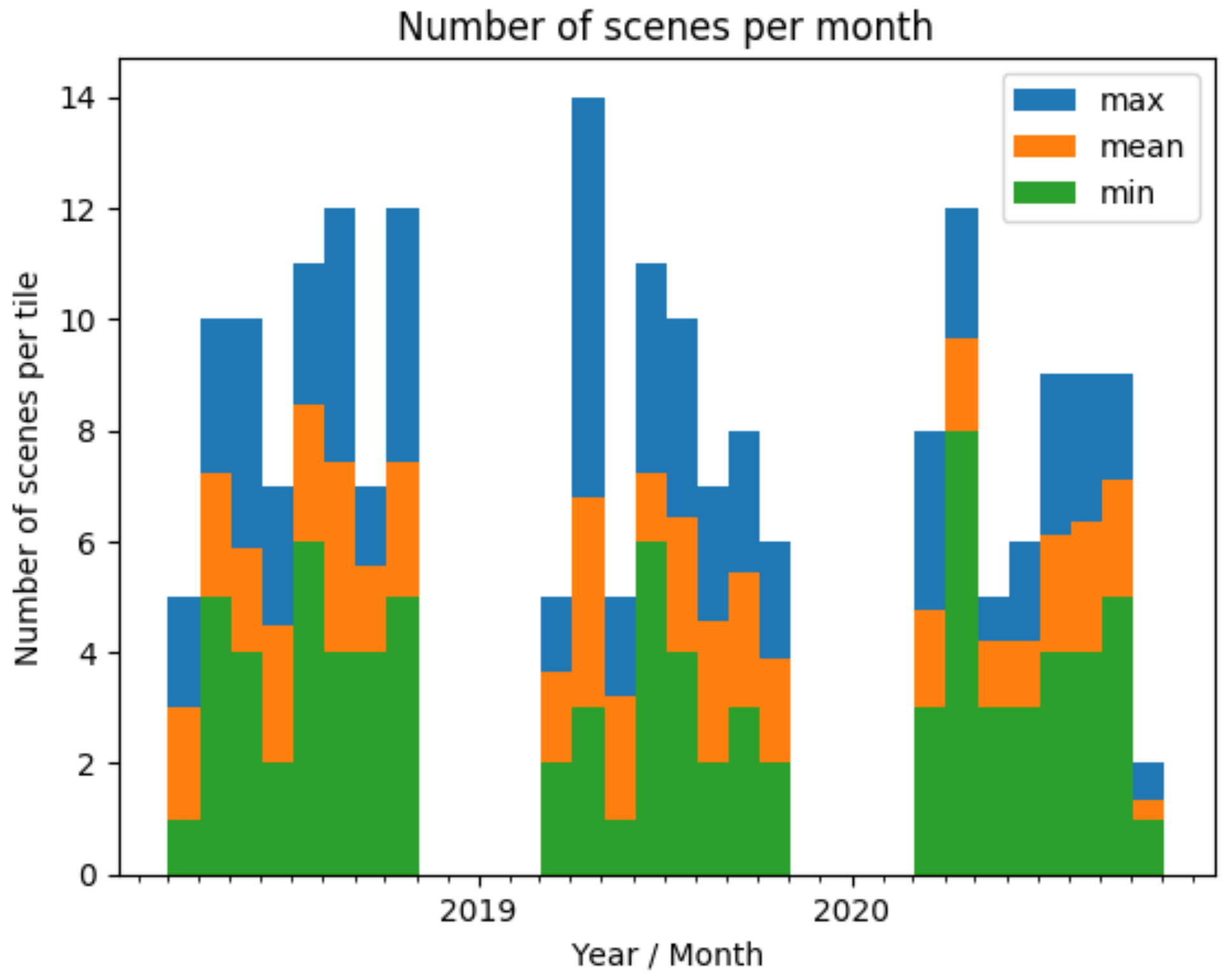
40]. For the nine tiles, statistics of the number of scenes per tile are given in
Figure 3. In 2018, the test site was characterised by arid and cloudless weather, which resulted in a constant high number of scenes across the observation window from March to October. The distribution of Sentinel-2 scenes per month and year shown in
Figure 3 in relation to the climatic conditions of the respective year gives the first view of potential soil conditions and, thus, SRC variability that is integrated into the SRCs. In total, 1202 single images are used from 2018 to 2020. The three Sentinel-2 bands with a pixel resolution of 60 m (B1, B9, B10) are excluded, while the four 10-m bands (B2, B3, B4 and B8) are resampled to 20 m pixel resolution using the nearest neighbour.
For generating SRCs, bottom-of-atmosphere reflectance data (L2A) and per-pixel cloud, haze and snow information are required. All orthorectified S2 data (L1C) available for the test site are downloaded, filtered by the constraint mentioned above and ingested into DLR’s internal processing environment. In the next step, L1C data are processed to L2A reflectances using MACCS-ATCOR Joint Algorithm (MAJA) [
41,
42].
2.3. Corine Land Cover (CLC) Data Processing
For the compositing approach (see
Section 2.6), SCMaP can assimilate two thresholds to separate bare soils from spectrally similar land cover (LC) types without using ancillary data [
15]. It requires understanding the temporal behaviour of certain LC types (see
Section 2.7). The Corine Land Cover (CLC) mapping is used to select the LC types of interest. It is a European-wide harmonised and long-term available LC database coordinated and integrated by EEA and available as a Copernicus service [
43]. It currently contains LC layers and change layers from 1990 to 2018 and will be regularly updated in the future. The long time for which CLC is available is used to calibrate the threshold model on stable areas across time. Thus, areas are excluded that had a recent change and might not be representative of the LC type.
In order to analyse the temporal behaviour of certain LC types, the CLC need to be filtered and aggregated according to the procedure described in [
30]. Bare soils most likely occur in agricultural areas after harvesting and before sowing. Therefore, all CLC types linked to intense agriculture have been combined and renamed crops (LC crops: combination from CLC classes 211, 212 and 213). NPV is known as spectrally similar to bare soils in multispectral EO data. This cover type mostly occurs in grasslands in a dry state and in deciduous forests when they are in a leaf-off condition. In order to analyse spectral-temporal NPV characteristics, grassland-type LC classes CLC 231, 321 and 322 are chosen and combined with LC grassland. Further, deciduous forests show NPV mostly in spring and autumn under leaf-off conditions. Therefore, CLC class 311 has been selected for LC deciduous. Spectral similarity can also be found in urban areas such as impervious surfaces, and thus CLC classes 111 and 121 are combined to build LC urban for this study.
For all available CLC surveys from 1990 to 2018, the described CLC classes are aggregated while keeping the vector format. Only areas that remain unchanged across all CLC surveys are used. Additionally, the CLC change layers (CHA) are used to filter our small-scale changes that are not covered by the general CLC surveys. Borders of 100 m are excluded from the stable LC pixel areas [
30]. In the final step, the vectors are rasterised in the same spatial resolution as the multitemporal S2 database (20 m). For the resulting stable LC pixels, the spectral-temporal characteristics are measured by spectral indices as the primary information for defining the thresholds (see
Table 1).
2.4. Lucas Soil Spectral Library (SSL)
The LUCAS Soil Spectral Library (SSL) is part of the Land Use/Cover Area frame Survey (LUCAS). It is the only existing European-wide soil, and landcover survey repeated regularly and measured in a standardised way [
44]. Besides chemical analyses, all soil samples are spectrally measured by a single laboratory. The LUCAS soil survey is updating our knowledge about the status and development of European soils. Further, it is an elementary part of the European soil mappings published regularly by the Joint Research Center (JRC). In this study, the SRC spectra are compared to the LUCAS SSL spectra of 2015 to evaluate the spectral performance of the SRCs and their potential for further European-wide soil modelling and prediction. However, the SRC spectra are a collection of natural soil conditions containing different roughness and moisture conditions. In contrast, LUCAS SSL contains spectra measured in oven-dried and sieved conditions. Since it can be expected that this treatment mainly impacts the albedo and that spectral absorption features of mineral components remain, LUCAS and SRC spectra are compared using the spectral angle (see
Section 2.8).
The LUCAS spectra were resampled to S2A/(B) L2A reflectances using the following formula (see also [
45]):
where
corresponds to the LUCAS spectra,
to the response function for each of the S2 bands and
is the band integrated reflectance value. The spectral response functions from S2 bands are taken from ESA’s web resource [
46].
2.5. European IACS Data
The Integrated Administration and Control System (IACS) of the European Commission (EC) is the main pillar of controlling European payments to farmers. One of the elements is a spatial database for all agricultural plots (land parcels) in EU countries for which payments have been made. The IACS mapping and database are controlled by independent facilities on behalf of the EC. For each year, land parcel outlines are stored with information about the broad crop category (arable land, grassland, permanent crops, permanent grassland, others) and the specific crop type harvested in the respective year. In this study, a subset of the IACS database for 2018, 2019 and 2020 covering the test area of Bavaria, Germany, is used to validate the SRC bare soil mask. The mask contains the coverage of the SRC pixels. The validation is based on the assumption that the SRC shall cover crop types with a harvesting event in the respective year since they will appear in bare soil conditions. Therefore, all areas covering a crop type with a harvest event within the period of interest are collected in the bare soil mask representing the ground truth for the spatial representation of the SRC pixels. In this study, three years from 2018–2020 are integrated to build the IACS bare soil mask for comparison with the SRC mask of bare soils.
2.6. Soil Composite Mapping Processor (SCMaP) Update
The generation of the SRCs follows the principles published in [
15] and is developed to analyse multitemporal Landsat databases. It computes several temporal, spectral and index composites, frequency products and statistical products from a multispectral image time series that can support digital soil mapping and spectral soil modelling. The main output is the SRC that collects predominantly pure bare soil pixels from a multispectral time stack. The development of SCMaP started with Landsat data inputs and is now extended to using other multispectral multitemporal data cubes, such as Sentinel-2.
SCMaP has been primarily developed for temperate and continental climates, where bare soils occur mainly in agricultural areas. These areas are characterised by a change from the vegetated condition during the green-up and crop growing stages to bareness after harvesting and when fields are in the seedbed condition. The frequency and time of bareness depend on the crop cycle. After filtering out cloud pixels and snow pixels using the normalised difference snow index (NDSI), SCMaP computes a spectral index (see
Table 1) for each scene and calculates the minimum and maximum index composites. These index composites are used for the index threshold derivation described in
Section 2.7. SCMaP uses two spectral index thresholds (
,
) to separate non-vegetated areas from vegetated areas in every single scene of the temporal data stack. Only pixels showing a change between vegetated and non-vegetated states are recognised as bare soil pixels. These pixels are different from permanently sealed surfaces. The number of required changes can be defined as (
). It mitigates the effect of spurious outliers and allows the computation of meaningful quality layers, such as the standard deviation (
s) of the SRC spectra. It should be noted that the SCMaP principle differs from other techniques that use ancillary data to exclude other areas such as urban or permanent vegetation (e.g., [
18]).
The processor can handle different spectral indices.
Table 1 provides an overview of the spectral indices that are used in this study. NDVI and NBR2 are selected because they are the most commonly used indices described in the literature. PV+IR2 combines information from the VNIR and the SWIR wavelength region. Both regions are relevant to separating green vegetation and NPV from bare soils. The SCMaP has been used for the generation of all compositing image products with varying parameter settings that are described in
Section 3.1.
Table 1.
Spectral indices used by the SCMaP in this study.
Table 1.
Spectral indices used by the SCMaP in this study.
| Index Name | Index Short | Formula | Reference |
|---|
| Normalised Difference Snow Index | NDSI | (B3 − B11)/(B3 + B11) | [47] |
| Normalised Difference Vegetation Index | NDVI | (B4 − B8)/(B4 + B8) | [48] |
| Combined NDVI and SWIR2 index | PV + IR2 | (B8 − B4)/(B8 + B4) + (B8 − B12)/(B8 + B12) | experimental |
| Normalised Burned Ratio 2 | NBR2 | (B11 − B12)/(B11 + B12) | [49] |
2.7. Histogram SEparation Threshold (HISET) Method
Two spectral index thresholds are used to separate bare soils from all other surfaces. In the case of SCMaP, the histograms of the minimum and maximum index composites (
Section 2.6) for all stable LC pixels (
Section 2.3) are used to analyse their spectral-temporal characteristics. To separate bare soils from vegetation, especially when NPV dominates vegetation, histograms of the minimum index composite for crops and grassland/deciduous are used. The separation of bare soils and urban areas is based on the histograms of the maximum index composite for crops and urban areas. In both cases, the histograms of the respective LC types overlap and prevent full separation. In order to remain flexible in the choice of the used index and regional specifications, a new strategy has been developed that can separate two LCs with minimum overlap between them. The threshold is based on the optimal separation of two histograms and, therefore, is called the HIstogram SEparation Threshold (HISET). The following calculations are performed iteratively over the range of the two input histograms or probability density functions (PDF) to calculate the HISET and the corresponding HISET score (see also
Appendix A.1):
For each of the histograms/PDFs, the proportion of the bins left and right of a potential threshold is calculated.
For the two calculated proportions on each side of the threshold, the minimum is determined.
The maximum of the two minima is determined for the potential threshold (preliminary HISET score).
The final HISET score is defined by the minimum of all the calculated scores in the previous step. This minimum also determines the final histogram separation threshold.
The resulting HISET score is a quality measure describing how well the two input histograms could be separated. It can be described as the smallest possible proportion of any distribution of A lying on the same side of the threshold as distribution B while making sure that distribution B does not have a higher proportion lying on the other side of the threshold than distribution A. For a threshold separating the two histograms completely, the HISET score would be 0%. For the worst realistic separation, for example, for two identical histograms that cannot be isolated, the HISET score would be approximately 50%. For example, a worse score is possible in theory for two identical histograms containing only one bin. For the presented use case, however, realistically, this should never occur.
It is worth mentioning that it makes no difference for the HISET algorithm if the provided inputs are histograms or PDFs since it works with proportions. For a graphical representation of the threshold together with the two distributions, however, it makes sense to use the PDFs, especially if the relative size of the two distributions varies significantly.
2.8. Spatial and Spectral Performance Assessment
The SRCs have been proven as a suitable database for large-scale soil modelling [
18,
25], and their quality has been mostly assessed indirectly by metrics describing the resulting soil parameter prediction. Commonly, they are calculated as the coefficient of determination (R2), the root mean square error (RMSE), the performance of deviation (RPD) and the ratio of performance to interquartile distance (RPIQCV), indicating the model and the prediction performance [
22,
34,
50,
51]. The quality of the underlying SRCs is not explicitly evaluated. The best way to express and compare the quality of an SRC product is to calculate its uncertainty. Although it is a standard for single-pixel measurements [
52,
53] that include uncertainties due to atmospheric parameters, such as aerosol optical thickness or water vapour, the uncertainty is even more complex for a pixel-by-pixel combination of spectra collected over time. The observed surface has its own spectral, spatial and temporal variability and, thus, sources of uncertainty [
54]. Even more, temporal compositing can depend on varying cloud and snow cover. Thus, temporal data integration is not equal across space, leading to sampling uncertainty [
55].
To the authors’ knowledge, there is currently no standardised procedure or set of measures to evaluate the accuracy or uncertainty of temporal bare SRCs in terms of spectral agreement with a reference soil measurement. Due to the lack of a statistically reliable number of matching in situ and S2 spectral measurements, the focus of this study is on spectral and spatial metrics (
Section 2.8.1 and
Section 2.8.3), enabling a comparison of different SRCs and proving a pixel-wise estimate of the variability and confidence of the resulting SRC spectra (
Section 2.8.4). Further, the spatial coverage of the bare soil pixels (bare soil mask) is validated against the IACS database (
Section 2.8.2).
2.8.1. Spatial Performance
The percentage of bare soil pixels is a general measure to assess the spatial coverage for which soil parameters can be directly derived from EO data using spectral soil modelling approaches. Especially for large-scale soil modelling (e.g., Europe) that is dependent on sparsely distributed calibration points derived from standardised soil core measurements, a higher SRC coverage can be essential for higher model performance. Thus, the percentage of bare soil pixels and the number of LUCAS points counted that are covered by the SRC.
2.8.2. Spatial Validation of the Bare Soil Mask
However, the percentage of bare soil pixels is not suitable to assess the spatial validity and completeness of the bare soil area since spectrally similar surfaces, such as deciduous forests in leaf-off conditions or NPV-containing grasslands, might be detected as bare soils due to the spectral similarities [
56]. Few authors have presented spatial metrics such as the percentage of detected bare soil area and the spatial agreement of the bare soil area with the crop area [
18,
28,
30]. The latter is especially applicable in the temperate climate zone, where bare soil occurs mainly during harvesting and ploughing of agricultural sites and barely on natural sites.
The external IACS database containing land parcel-specific crop types has been used for the quantitative validation of the bare soil area. It is a European database containing all agriculturally used areas and is updated yearly (see
Section 2.5). The derived mask of bare soils is compared to the bare soil mask of the SRCs to perform a simple pixel-wise accuracy assessment. It comprises true and false positives and true and false negatives for the entire test area available as an image product and as a confusion matrix (
Figure 4).
2.8.3. Spectral Performance
The quality of the spectral representation of the SRCs is essential for calibrating the soil spectral models. However, the assessment of the quality is not trivial. A composite spectrum integrates different natural conditions over the selected time range. In the case of soils, the spectrum changes with different soil moisture contents, roughness conditions and other disturbance factors such as NPV coverage that can only be minimised by using multispectral data for generating spectral composites. For optimal soil modelling, the soil condition would be dry, and the surface is smoothed because calibration points available on a large scale, such as LUCAS, are measured under laboratory conditions (dried and sieved). Such soil conditions rarely occur in natural environments. Therefore, the spectral comparison will be affected by albedo differences. Ref. [
14] compared laboratory and composite spectra using derivatives such as the soil line and dispersion between selective bands using principal components for both laboratory and composite spectra. In a preliminary study, Ref. [
57] used the spectral angle [
58] between LUCAS SSL spectra and the respective SRC spectra for estimating the similarity of the spectral pairs by neglecting albedo differences. Although these spectral similarity measures are not suitable for estimating absolute spectral agreements, they can be used to evaluate the improvement or degradation of SRCs generated by varying processing parameters. In order to compare the spectral performance of the different SRCs, the spectral similarity between the spectral lab measurement of the LUCAS points and the SRC spectra is calculated using the
spectral angle. The spectral angle has been widely used in geological hyperspectral applications and is known to be insensitive to illumination and albedo effects [
58]. The band-wise
mean reflectance difference between both measurements is additionally calculated for completeness.
2.8.4. Spectral Variance of SRCs
Due to the averaging of several bare soil measurements in the SRC spectrum, different soil conditions are covered, although there are concepts to reduce disturbing effects by choice of index, selection of specific seasons [
29] or the use of SAR data [
28] to account for soil moisture variability. Therefore, instead of getting a perfect Sentinel-2 spectrum, information about the spectral variance of the averaged soil conditions (
) and the standard deviation (
s) for each SRC spectrum (
) is calculated as:
The SRC pixel s is calculated using different composite parameters that can be considered a quality parameter for the resulting composites. Thus, the s is a parameter for evaluating the spectral variance within an SRC image, and it can reveal if natural patterns of variance exist, such as for field edges, where more spectral variability due to disturbances from, e.g., NPV, can be expected.
However, the spatial representation of
s can be biased by the number of
valid pixels used for the SRC averaging. For each SRC, per-pixel information about the number of valid bare soil observations is stored in an image product. The number mostly depends on cloud, haze, snow coverage and the geographical position on Earth. On the one hand, there is a higher overlap of S2 orbits in higher latitudes resulting in denser time series, but on the other hand, the large-scale probability of cloud-free images is decreased. The general assumption is that the more pixels are available, the more soil conditions are integrated into the mean SRC pixel spectrum. A higher number of valid pixels can be positive because it increases the confidence and reliability of the averaged SRC spectrum. However, this increases the likelihood of integrating more outliers in the pixel spectrum, such as more moisture levels. Ref. [
29] found that instead of integrating all available bare soil conditions, carefully selected observations, predominantly before the green-up phase where soils are smoothed and dry, can result in higher SOC prediction performances. In this study, the minimum number of valid pixels is set to three observations to reduce the number of extremes and outliers. For comparing SRCs generated by the different processing parameters, the minimum (
), maximum (
), mean (
) and standard deviation (
s) are calculated for the complete area of the SRCs, additionally to the pixel-based image product.
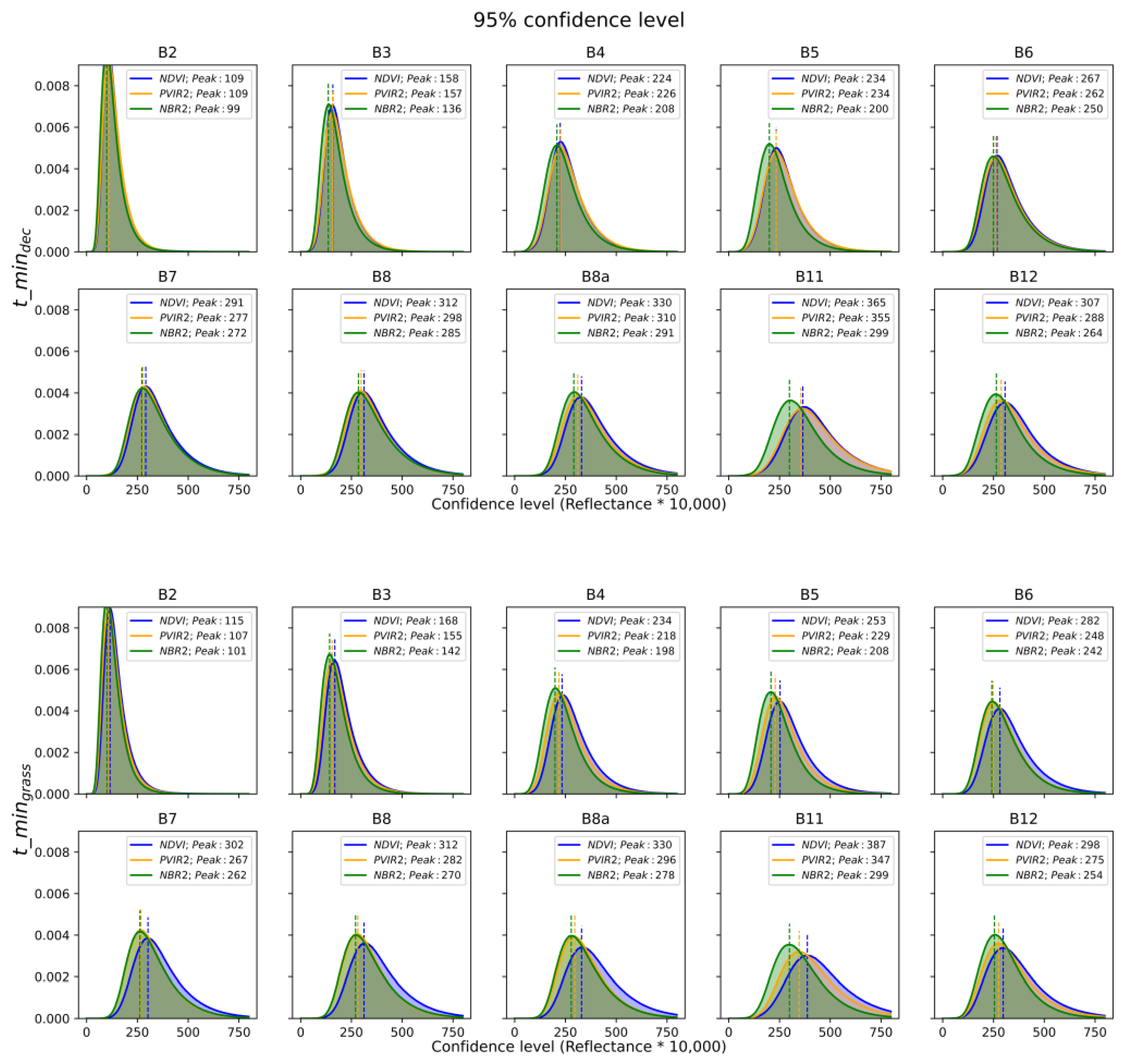
Finally, the 95% confidence interval (CI) of the SRC spectrum (
) is a measure for estimating the uncertainty of this pixel spectrum [
59]. The measure can be taken as quality criteria for a potential calibration point selection. The CI for each spectral band is defined as:
where
is 0.05, df is the degrees of freedom, defined as n − 1,
n is the number of reflectance values and
t is the
t-value, which is 2.093 for the 95% CI.
3. Results
3.1. Experimental Settings
Six SRCs have been created using three indices (see
Table 2) and two
threshold versions. The thresholds vary according to the results of the HISET analysis described in
Section 3.2. The processing parameters for each SRC are listed in
Table 2.
3.2. Thresholds
The
and
index composites have been processed for each spectral index (NDVI, PV+IR2 and NBR2) and per S2 tile (see also
Table 2). HISET thresholds and scores are derived for each of the S2 tiles and for a spatial mosaic of all tiles.
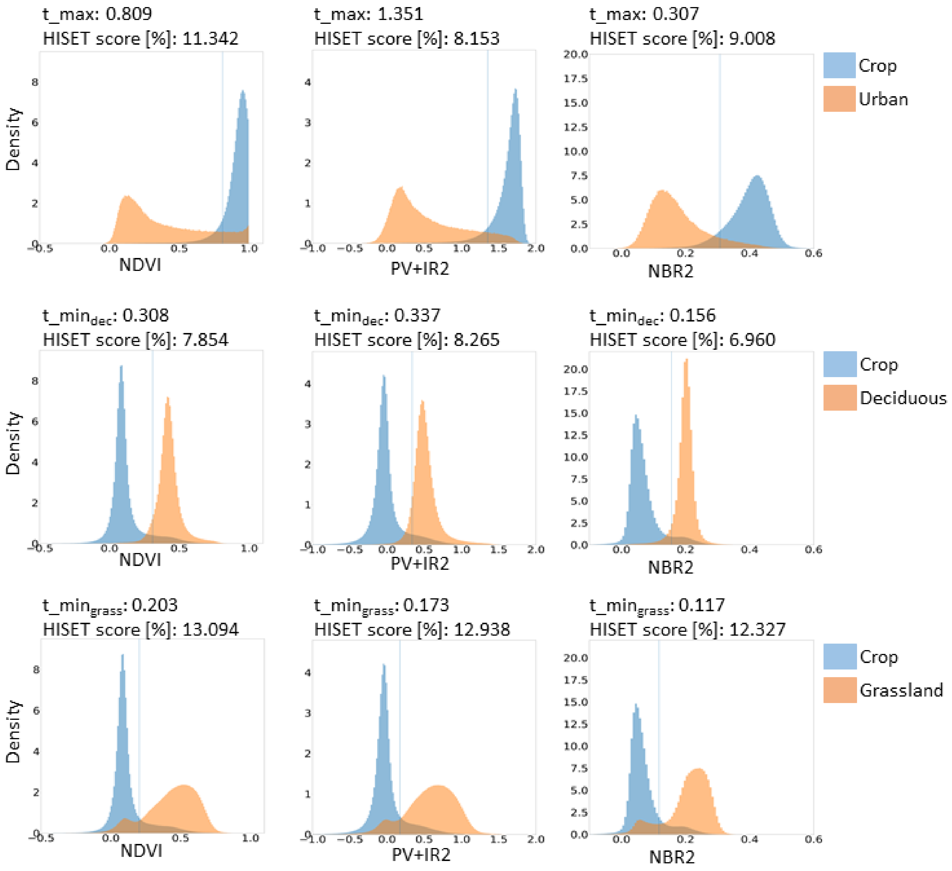
Figure 5 shows the histogram plots for all pixels covering the selected LC types in the complete test area. For
t_
, the crop pixels are compared with the urban pixels.
has been created in two versions, (1) by comparing crops with deciduous trees and (2) by comparing crops with grassland.
Figure 5 shows histogram overlaps for all indices and thresholds. For calculating
t_
, the
index composite is used, where crops shall be in a photosynthetic-active state and, therefore, well separable from urban areas (upper row). The overlap happens when urban LC pixels are also covering urban green. The HISET score for PV+IR2 is 8.2% and, thus, has the lowest score value. The highest score can be found for NDVI (11.3%). Independent from the index, deciduous (middle row) and grassland (lower row)
index values show clear differences. Compared to grasslands, histograms of deciduous show minor overlaps, resulting in thresholds with HISET scores between 7.0% and 8.3%. For grassland, a bimodal and wider distribution of index values can be observed for all indices. It highlights the above-described spectral similarity of NPV and bare soil that cannot be fully separated using multispectral data, especially when the NPV-containing LC is in a dry condition (first local maximum). Although the HISET score is higher than for deciduous trees, each index’s threshold is defined as lower, resulting in fewer pixels that are selected for building the SRC. Thus, fewer disturbance effects are expected. Comparing the three used spectral indices, the HISET score for NBR2 is the lowest for both
versions.
In the next step, the derived HISET thresholds and scores have been analysed to reveal potential dependencies on specific LC characteristics of each S2 tile. The
distribution pattern (left column of
Figure 6) is similar for NDVI and PV+IR2 since the index calculation is similar (see
Table 1). At the same time, values for S2 tile 32UPA are the lowest for each of the indices. Threshold differences between
and
are obvious, and similarities between NDVI and PV+IR2 are visible. NBR2 shows different spatial patterns for both
versions. An S2 tile-based variability of HISET scores can also be observed (see
Figure A1). To clarify, if the derived HISET values are related to the percentage of occurring LC type pixels, a preliminary multiple regression analysis (MRA) has been performed by defining the HISET score or threshold as a predictor and the two respective LC types as coefficients. The test has been performed by considering all nine S2 tiles. The coefficients of determination, R
2, for all tests are below 0.52, with a mean R
2 for all thresholds and indices of 0.30. The results show no measurable relationship between the percentages of LC types used to derive the HISET parameter.
3.3. Composite Generation
Based on the threshold analyses described above, the
and
index values have been derived for each spectral index for the complete test site (9 tiles = 95.964 km
2). The SRCs are processed using the
and
listed in
Figure 5. The performance of each resulting SRC is quantified using the methods described in
Section 2.8, and the image-based results are summarised in
Table 3.
Figure 7 shows an SRC subset around Noerdlingen, Germany, generated from PV+IR2 and using
. Additionally, two example subsets, A and B, for all processed versions (see
Table 3) are displayed for various image data products. The colour stretching is equal for each row of the example subsets to enable the visual comparison of the image results.
Compared with the WRB soil types, the area East of the city of Noerdlingen, Germany (example A), is covered by luvisols and appears reddish in the images. West of the river Woeritz (example B), the images have a greenish colour. Cambisols and stagnisols cover these areas.
A closer look at examples A and B shows that the resulting composites differ in spatial coverage and spectral variability, driven by the selection of the number and type of valid pixels. In principle, the number of valid pixels is higher for all
versions independent from the index. This is in line with the generally lower threshold values for the
listed in
Table 3. Since the valid pixel images show patterns related to the fields, it can be assumed that the occurrence of bare soil pixels is related to the crop type. This effect is visible for each of the indices and
versions. In the examples in
Figure 7, the NBR2/
parameter combination produces the least coverage of SRC pixels. However, for the entire test side, the PV+IR2/
combination shows the lowest coverage of bare soil pixels (
Table 3), while the mean number of valid pixels is slightly higher compared to NBR2/
(16.19% vs. 15.76%). From all
versions, NBR2 resulted in the highest coverage of bare soil pixels (29.64%). The number of LUCAS points that are covered by the SRCs is similar for
and
versions, respectively.
3.4. Performance Assessment
As expected from
Section 3.2, SRCs generated using
have a lower percentage of exposed soils than those processed with
due to the more strict threshold value. The SRCs generated using the NBR2 cover the largest percentage of exposed soils. However, values between the index versions differ less than between
versions. Interestingly, the mean number of valid observations is highest for the NDVI thresholds, indicating that the NDVI threshold allows more pixels to be integrated with the SRC pixels. The most restricted selection of valid pixels is performed for the NBR2/
version. The spectral comparison between S2 resampled LUCAS and SRC spectra using the spectral angle and the mean reflectance difference (
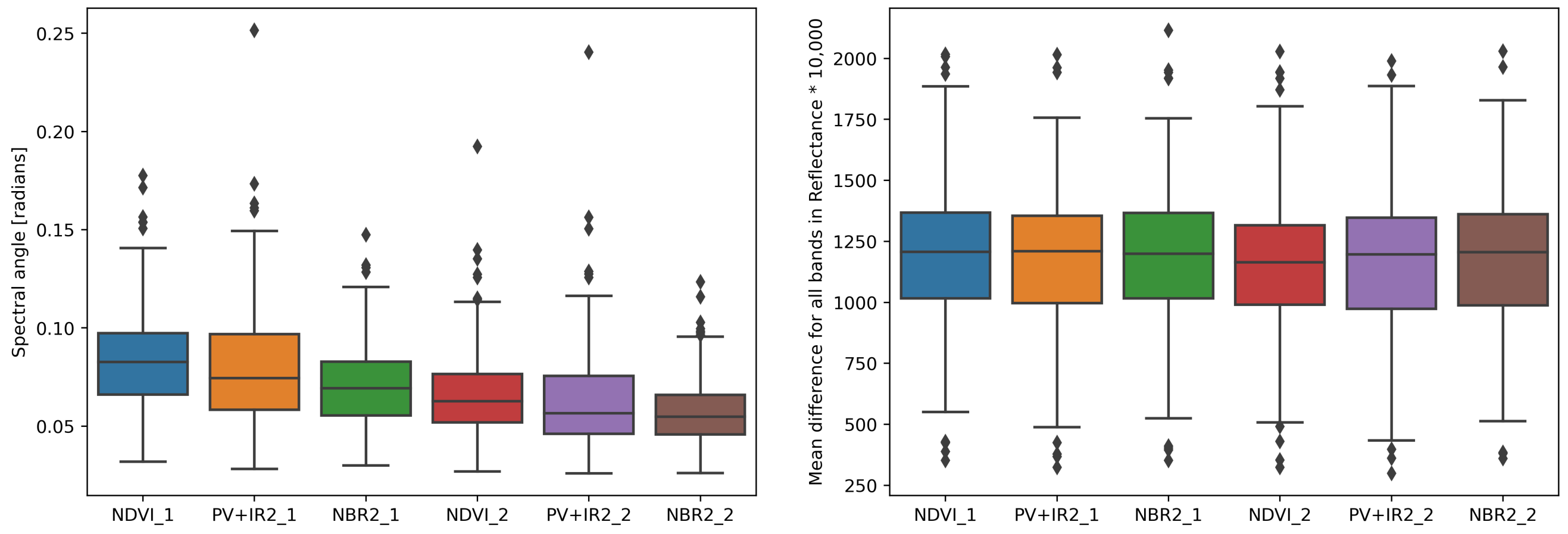
Section 2.8.3) was made for all LUCAS points that cover an SRC pixel. Further, only those LUCAS points are considered that are covered in every SRC to ensure the comparability of the spectral angle and mean reflectance difference values.
Figure 8 presents a comparative view of the statistic.
The summarised spectral angle statistics show a gradient from NDVI, PV+IR2 to NBR2 for all versions. The best match can be found for the NBR2/ version with a mean spectral angle of 0.058, which marks a drop of more than 30% compared to the highest spectral angle value calculated for the NDVI/ version. Additionally, the interquartile range of SRC/ versions is smaller compared to the SRC/ versions, with the smallest interquartile range of the NBR2/ SRC. In contrast, the calculated mean reflectance differences do not show significant changes across the SCR versions.
3.5. Validating the Bare Soil Mask
The bare soil mask built during the SCMaP processing collects pixel positions showing bare soils between March 2018 and October 2020 (excluding winter months). This bare soil mask has been validated using the preprocessed IACS data (see
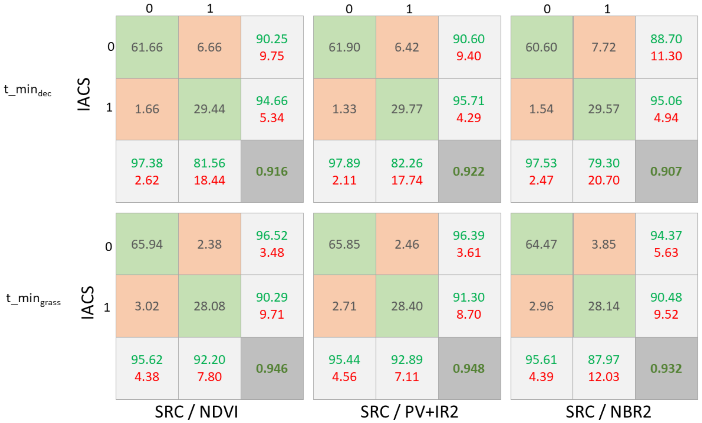
Section 2.5) that contains the same information as the SCMaP bare soil mask. Therefore, the validation is a pixel-based comparison of both masks to quantify their agreement. Both binary masks cover the same spatial extent, determined by the common overlap between the IACS and the SRC data. This analysis has been performed for the six SRC versions resulting in six confusion matrices, where grey numbers in the coloured boxes are given in the percentage of matched/unmatched pixels (
Figure 9). The most crucial target, class 1, represents bare soils, whereas class 0 collects crops with permanent vegetation coverage. The accuracy of class 1 is measured by true negatives (TN), according to
Figure 4.
The overall accuracy for all index/ versions is >0.9 for all six SRCs. The versions have higher accuracies than for all versions. Most important are the matrix values of the middle quarter at the bottom that summarizes the percentage of SRC pixels also covered by the IACS mask (TN as the green number). In the same box, the percentage of SRC pixels not covered by the IACS mask is listed (FN as the red number). While the mean number of valid pixels is always higher for all versions in comparison with the version, the TN percentages are lower and more misclassification occurs. In return, the version shows less misclassification for all indices. Comparing the three indices, PV+IR2 seems to perform best, and NBR2 has the lowest accuracy values.
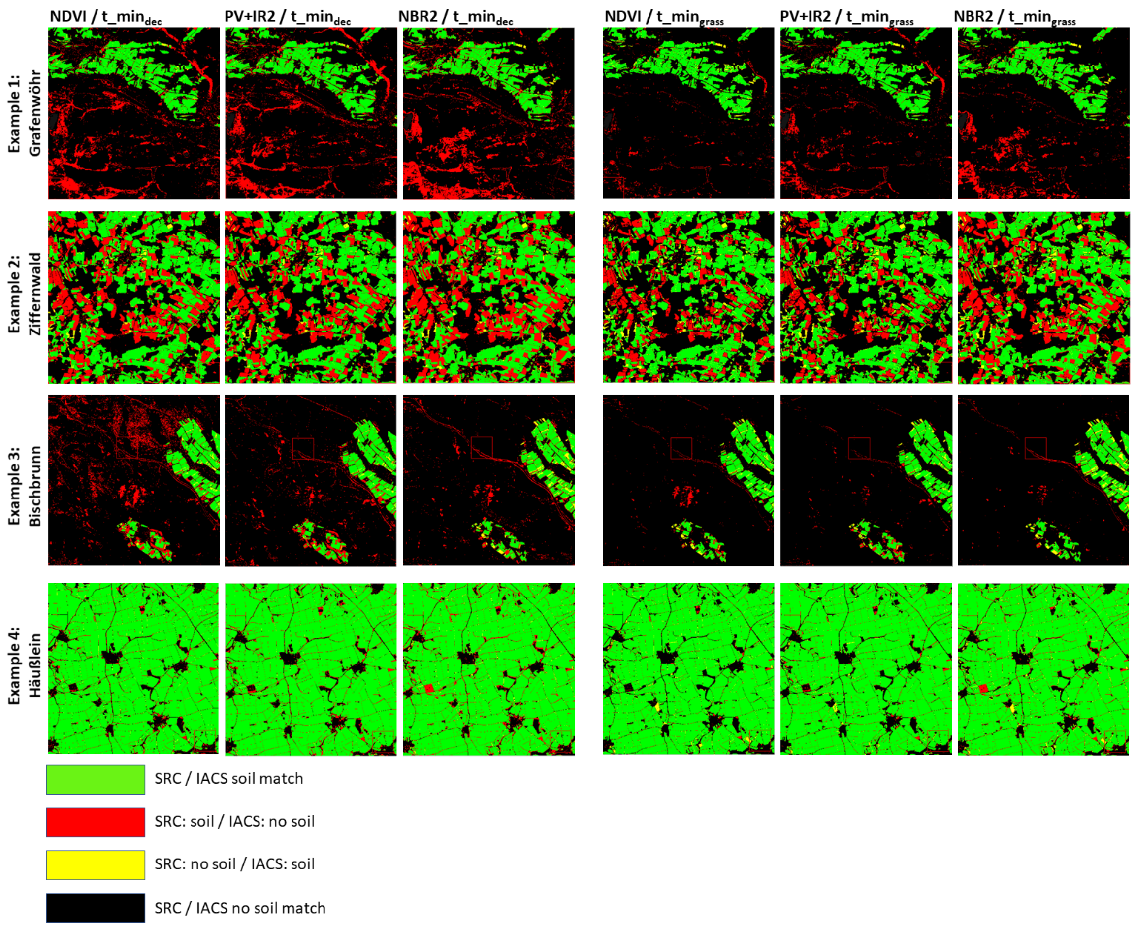
However, since the overall accuracy numbers are similar for all index/
versions,
Figure 10 selects some image examples that mainly visualize problematic areas. Example one shows an area around the military area, Grafenwoehr, Germany, with crops limited by grassland along the river Creussen in the North and a mixture of natural grasslands, open soil surfaces and mixed forests in the Southern part of the image. This example highlights that stricter thresholds such as
improve the exclusion of NPV, such as grassland and peatland in the military area. However, it also contains a few real bare soil surfaces correctly identified. In general, it can be observed that NBR2 is strong for detecting and excluding pure NPV surfaces (such as along river Creussen in the North) but fail for peat bog areas (e.g., Southern end of the example image). If mixtures of NPV, bare soils and photosynthetic-active vegetation are present, NDVI-based indices perform better.
In the second example, the area is dominated by crops. None of the indices and versions seems to work correctly. The red fields are not in the IACS mask because they are classified as permanent crops. These crop types are excluded from the IACS mask. However, the area is dominated by hope cultivation characterised by bare soil exposure in the spring month before the green-up phase. Those areas are correctly detected as bare soils within the SRCs.
Example three shows the area Northwest of the small town of Bischbrunn at the Spessart, rich in old deciduous forests (a mixture of oak, beech, larch and other tree types). Specifically, the NDVI/ version seems to fail here. In all versions, deciduous trees could be correctly excluded from the SRCs.
Opposite to the above-described three examples, example four shows purely crops, where SRC and IACS mask mainly match. The versions show a few yellow pixels highlighting areas where SRC did not contain bare soils, while IACS expects it.
3.6. Spectral Variability of SRCs
In the logic of a perfect spectrum as input for spectral modelling, the soil measured by an EO instrument shall be dry and smooth to be comparable with laboratory measurements of a soil parameter, such as soil organic carbon. In this case, the spectral variability of the SRC would be very low. However, this is very unlikely to occur in natural environments. In
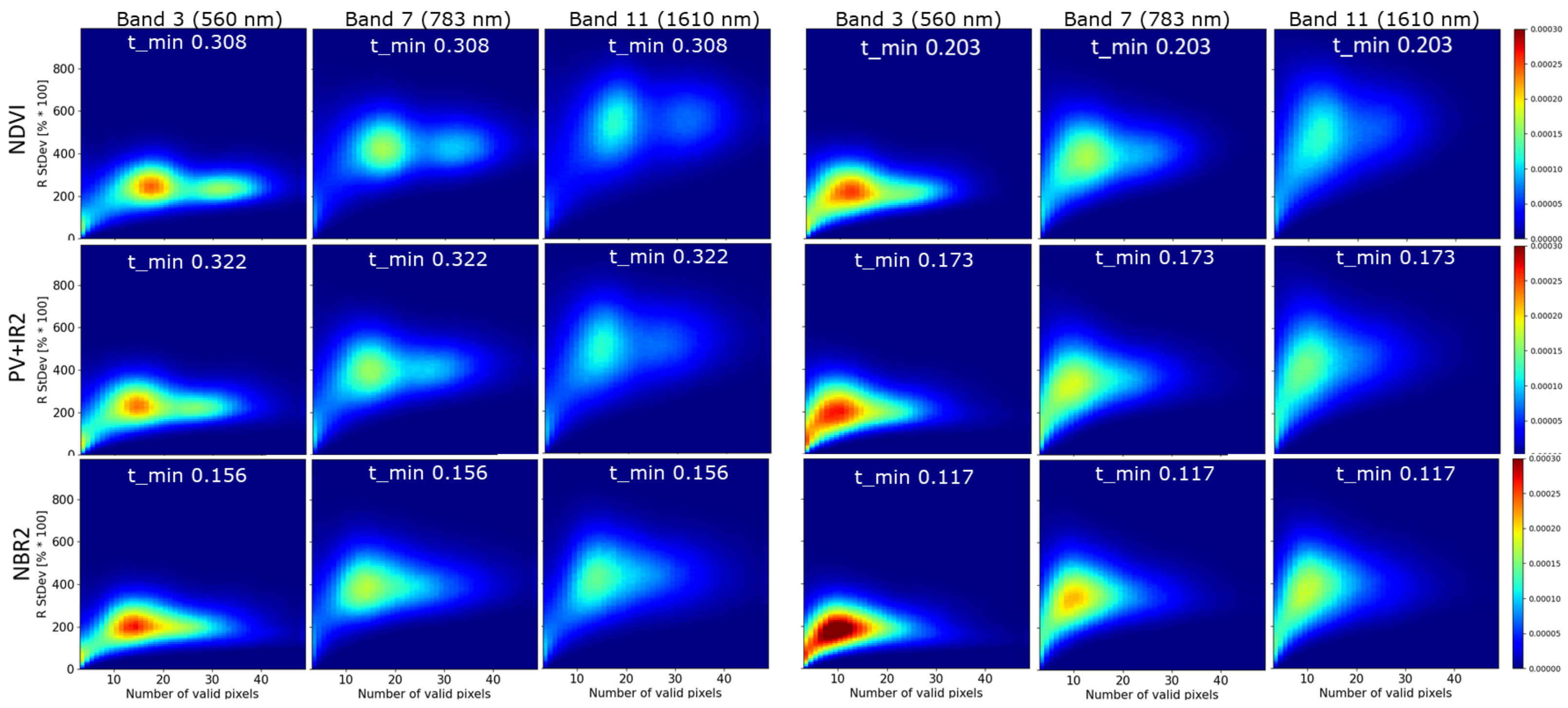
Figure 11, the pixel-based spectral variability is shown for each SRC version as a function of the number of valid pixels for three selected S2 bands.
Since s depends on the mean SRC reflectance, it is low in bands where the reflectance is also low for soils. Band 11 shows higher s values than band 3. At the same time, the spread of values is higher for higher band numbers. The majority of pixels have a s around 1–3% for band 3, around 4% for band 7 and 4–6% for band 11. Concerning the number of valid pixels, s values seem to achieve an equilibrium, where the mean s values are not increasing anymore with the number of valid pixels. Moreover, the variability is getting smaller, indicating that all soil conditions are integrated into the SRC reflectance. Comparing the three index versions, the state of equilibrium gets higher with the bands and shows a slight decrease from NDVI to NBR2. The same can be observed at the versions. However, the s hotspot and the number of valid pixels are lower for all bands.
For a more generic view of the dependency of the number of valid pixels and
s, the 95% CI per used S2 bands for all SRCs is estimated (
Figure 12). Image histograms were calculated with a bin size of 75. For comparison, histograms are normalised such that the total area of the histogram equals 1. The CIs differ per spectral index and
SRC version, but they simultaneously vary per band. The largest CI differences can be seen at band 11, followed by bands 5, 8a and 12. The CI of NBR2 is the lowest in almost all bands and all
SRC versions. The
SRC versions show a gradient from NDVI with the highest to NBR2 with the lowest CI. For bands 2, 6, 7, 8 and 8a, the PV+IR2 and NBR2 histograms match. In
Figure 7, the CIs are displayed for two example regions. It shows field-to-field differences as well as higher values at the field edges. Further, NBR2 has the lowest CI for both
SRC versions.

 ,
, 


