Tensor Dictionary Self-Taught Learning Classification Method for Hyperspectral Image

Abstract

Precise object classification based on Hyperspectral imagery with limited training data presents a challenging task. We propose a tensor-based dictionary self-taught learning (TDSL) classification method to provide some insight into these challenges. The idea of TDSL is to utilize a small amount of unlabeled data to improve the supervised classification. The TDSL trains tensor feature extractors from unlabeled data, extracts joint spectral-spatial tensor features and performs classification on the labeled data set. These two data sets can be gathered over different scenes even by different sensors. Therefore, TDSL can complete cross-scene and cross-sensor classification tasks. For training tensor feature extractors on unlabeled data, we propose a sparse tensor-based dictionary learning algorithm for three-dimensional samples. In the algorithm, we initialize dictionaries using Tucker decomposition and update these dictionaries based on the K higher-order singular value decomposition. These dictionaries are feature extractors, which are used to extract sparse joint spectral-spatial tensor features on the labeled data set. To provide classification results, the support vector machine as the classifier is applied to the tensor features. The TDSL with the majority vote (TDSLMV) can reduce the misclassified pixels in homogenous regions and at the edges of different homogenous regions, which further refines the classification. The proposed methods are evaluated on Indian Pines, Pavia University, and Houston2013 datasets. The classification results show that TDSLMV achieves as high as $99.13\%$, $99.28\%$, and $99.76\%$ accuracies, respectively. Compared with several state-of-the-art methods, the classification accuracies of the proposed methods are improved by at least $2.5\%$.

1. Introduction

Hyperspectral images (HSIs) are special images gathered from satellites or airplanes, which not only contain spatial pixels but also contain hundreds of spectral bands with every pixel. Because of consisting of abundant information, hyperspectral image (HSI) is wildly used in remote sensing fields [1,2,3,4,5,6], such as environment monitoring [1], urban mapping [2], land use analysis [4], and military affairs [6]. Among these applications, HSI classification is a basic task, which involves assigning class labels to pixels [7,8] and implements pixel-wise classification. Therefore, HSI classification has aroused a lot of interest from researchers.

Classification tasks require quantities of training samples. According to the annotation of training data, classification methods are divided into supervised learning, unsupervised learning, semi-supervised learning, transfer learning, and self-taught learning methods. Unsupervised learning methods just utilize unlabeled data. Therefore, they can extract features, but can not give the category labels for the testing data, such as principal component analysis (PCA) [9], independent component analysis [10], Gabor [11], sparse representation [12,13,14,15], and autoencoders [16]. On the contrary, supervised learning methods utilize labeled data to extract features and provide the category labels of testing samples, such as support vector machine (SVM) [17], and deep learning methods (i.e., convolutional neural networks (CNN) [7,18,19,20,21,22,23,24,25], recurrent neural networks (RNN) [26,27], graph convolutional networks [28,29,30,31], transformers [32], generative adversarial networks [33]). Semi-supervised learning methods [34,35,36] offer a solution to overcome the limited labeled samples problem by combining the power of labeled and unlabeled data information at the same time [37], such as active learning [38,39], and some extended methods for unsupervised learning [37]. However, semi-supervised learning typically makes the additional assumption that the unlabeled data can be labeled with the same labels as the classification task, and these labels are merely unobserved [40]. Transfer learning methods [41,42,43,44,45,46,47] utilize extra labeled data from the source data set to improve the supervised classification of target data. Moreover, the two data sets do not need to contain the same categories, but the source data needs to be related to the target data. Since the annotation of HSI is difficult and expensive to acquire, the self-taught learning methods [40] are more advantageous. Self-taught learning methods [8,48] utilize unsupervised learning on other unlabeled data to improve the performance of supervised classification.

Because the HSI contains both spatial and spectral information, the HSI classification methods can be divided according to the utilization of information. The early studies just utilize spectral information to classify every pixel, such as SVM [17], spectral sparse representation [12], one-dimensional CNN (1-D CNN) [18], and RNN [26]. Afterward, many studies demonstrate that spatial information can improve the performance of HSI classification [49]. SVM applied to the contextual data, and SVM with composite kernels both can provide higher accuracies than SVM applied to the spectral data [50]. Furthermore, some researchers improve the sparse representation methods [51,52,53,54,55] with spatial constraints, including Laplacian sparsity [14,56], joint sparsity [14,15], and group-based sparsity [13]. Except for incorporating contextual information into spectral information, some researchers extract joint spectral-spatial features from three-dimensional (3-D) HSI samples directly to further improve the classification, such as 3-D CNN [7] and tensor-based sparse representation methods [57,58,59,60]. Roy et al. [22] propose a hybrid spectral CNN (HybridSN) classification method, which is a spectral-spatial 3-D CNN followed by spatial a 2-D CNN. The 3-D CNN facilitates the joint spectral-spatial feature extraction, the 2-D CNN reduces the complexity. Zhao et al. [57] decompose the group tensor into the intrinsic spectral tensor and the corresponding variation tensor via a low-rank tensor decomposition algorithm and then classify the intrinsic tensor with SVM. To classify HSI with limited training samples, He et al. [59] present a testing sample tensor as a linear combination of all the training sample tensors via low-rank tensor learning. Liu et al. [58] have proposed an extended ridge regression for multivariate labels by taking advantage of tensorial representation. In our previous works [61], we propose the atom-substitute tensor dictionary learning (ASTDL) algorithm to train sparse tensor feature extractors, furthermore, we propose ASTDL enhanced CNN (ASTDL-CNN) classification method and utilize a 2-D CNN to extract deep features from the sparse tensor features.

The aforementioned studies have demonstrated that the classification accuracies of spectral-spatial methods are superior to those of spectral methods. Especially, since the HSI is 3-D data, including one spectral dimension and two spatial dimensions, it is natural to treat the HSI as a 3-D cube or tensor [57,58,59,60,62]. Therefore, we study the HSI classification method based on tensor sparse representation to preserve the joint relationships of the spatial information and the spectral information. Furthermore, HSI data is limited, especially the data with annotation. It has great significance to study the HSI classification method with limited training data set. Therefore, we study the HSI classification method based on self-taught learning, which utilizes a small amount of unlabeled data to improve the supervised classification.

In this paper, we propose a tensor-based dictionary self-taught learning (TDSL) classification method for HSI. The other self-taught learning methods require a large quantity of unlabeled data [8,40,48]. Whereas, the proposed method utilizes a small amount of unlabeled data from other data sets to improve the supervised classification with a small labeled data set. The amount of unlabeled data required in the proposed method is much smaller than in the other self-taught learning methods [8,40,48]. We propose a sparse tensor-based dictionary learning (STDL) algorithm, to train tensorial feature extractors for 3-D samples on the unlabeled data set. The proposed STDL algorithm initializes dictionaries with Tucker decomposition (TKD) [63], and updates dictionaries based on the K higher-order singular value decomposition (K-HOSVD) algorithm [64,65]. Then, we extract sparse joint spectral-spatial tensor features on labeled data with the learned feature extractors. The supervised SVM is applied to these tensor features. Furthermore, to utilize the spatial information in the classification map obtained by TDSL, we add the majority vote followed by TDSL to refine the classification. The proposed TDSL with the majority vote (TDSLMV) can reduce the misclassification of pixels in homogenous regions and at the edges of different homogenous regions. The unlabeled data and the labeled data used in this method come from two data sets, which can be gathered over different scenes even by different sensors. For the different scenes, one can be the city, and the other one can be a valley. When the proposed method trains feature extractors on data of one scene and directly applies the trained feature extractors to a classification task over another scene, we definite it as a cross-scene classification. Therefore, TDSL can meet the cross-scene and cross-sensor classification tasks.

The proposed TDSL and TDSLMV are methods based on sparse representation. Different from the aforementioned sparse representation methods, the proposed methods utilize tensor techniques instead of vector and matrix techniques, and extract 3-D tensor features from 3-D sample cubes directly. The 3-D feature tensors preserve the joint spectral-spatial information, which facilitates the reduction in the requirement for training samples. ASTDL-CNN is a supervised method, while the proposed methods belong to self-taught learning methods. The proposed methods utilize a small amount of unlabeled data to improve classification performance. Compare with ASTDL-CNN, the proposed methods require less labeled data.

The main contributions of this paper are summarized as follows.

1.

A TDSL classification method is proposed for the HSI classification task with limited training data, and the TDSL can complete the cross-scene and cross-sensors classification tasks.

2.

A STDL algorithm is proposed for 3-D samples with two spatial dimensions and one spectral dimension, to train joint spectral-spatial tensor feature extractors. In the algorithm, we initialize dictionaries with TKD and update these dictionaries based on K-HOSVD.

3.

We add the majority vote followed by TDSL to improve the classification. The proposed TDSLMV utilizes the spatial information in the classification map of TDSL to effectively reduce the misclassified pixels in homogenous regions and at the edges of different homogenous regions.

4.

The classification performance of the proposed TDSLMV is qualitatively and quantitatively evaluated on Indian Pines, Pavia University, and Houston2013 datasets. The experimental results demonstrate a significant superiority over several state-of-the-art methods. Furthermore, the trained feature extractor models can be applied directly to a classification task on a new dataset, and achieve high precision classification.

The remainder of this paper is organized as follows. Section 2 briefly introduces the tensor notions and algebra first, and then introduces the related self-taught learning and tensor decomposition. In Section 3, first, we describe detailedly the proposed STDL algorithm and then present the proposed TDSL and TDSLMV classification methods. In Section 4, we perform a series of experiments on five wildly used benchmark data sets to analyze parameters in the proposed methods and evaluate the proposed methods compared with several state-of-the-art methods. Section 5 concludes this paper.

2. Related Works

In this section, we introduce the notions and algebra of tensors [62], first. Next, we describe the self-taught learning framework in brief [40]. Finally, we introduce the TKD and higher-order singular value decomposition (HOSVD) [62,63,66].

2.1. Notions and Algebra

Tensors are multidimensional arrays, and the number of dimensions for a tensor is its order or mode [62]. In this paper, a vector (the tensor of order one) is denoted as a boldface lowercase letter $a\in {\mathbb{R}}^{I_1}$. A matrix (the tensor of order two) is denoted as a boldface capital letter $A\in {\mathbb{R}}^{I_1\times I_2}$. A tensor of order N is denoted as an underlined boldface capital letter $\underline{A}\in {\mathbb{R}}^{I_1\times I_2\times \dots \times I_N}$. Furthermore, a scalar is denoted as a non-boldface letter a or A. Fixing every index of a tensor but one, we can obtain the vector-valued subtensors, which are defined as fibers. Whereas slices are the matrix-valued subtensors, defined by fixing all indexes but two.

The manipulation of reshaping tensors to vectors is called vectorization. The vectorization of a tensor $\underline{A}\in {\mathbb{R}}^{I_1\times I_2\times \dots \times I_N}$ is defined as $b=vec\left(\underline{A}\right)\in {\mathbb{R}}^{I_N{I}_{N-1}\dots I_1}$, and its entries can be calculated by:

$$b_{i_1+{\sum }_{k=2}^N\left[(i_k-1)I_1{I}_2{I}_{k-1}\right]}=a_{i_1{i}_2\dots i_N}.$$

(1)

Reshaping tensors to matrices is called matrix unfolding or matricization. The mode-n matricization of a tensor $\underline{A}\in {\mathbb{R}}^{I_1\times I_2\times \dots \times I_N}$ is denoted as $B=A_{\left(n\right)}\in {\mathbb{R}}^{I_n\times I_1{I}_2\dots I_{n-1}{I}_{n+1}...I_N}$, and its enters can be calculated by:

$$b_{i_{n}j}=a_{i_1{i}_2\dots i_N},$$

(2)

where, $j=(i_1-1)I_2\dots I_{n-1}{I}_{n+1}\dots I_N+\dots +(i_{N-1}-1)I_N+i_N$.

The mode-n product of a tensor $\underline{A}\in {\mathbb{R}}^{I_1\times I_2\times \dots \times I_N}$ with a matrix $B\in {\mathbb{R}}^{J_n\times I_n}$, denoted by $\underline{C}=\underline{A}{\times }_{n}B$, is calculated by the multiplication of all mode-n vector fibers with $B$. The entries of $\underline{C}\in {\mathbb{R}}^{I_1\times \dots I_{n-1}\times J_n\times I_{n+1}\times \dots \times I_N}$ is calculated by:

$$c_{i_1\dots i_{n-1}{j}_n{i}_{n+1}\dots i_N}=\sum _{i_n=1}^{I_n}{a}_{i_1\dots i_{n-1}{i}_n{i}_{n+1}\dots i_N}{b}_{j_n{i}_n}.$$

(3)

The outer product of a tensor $\underline{A}\in {\mathbb{R}}^{I_1\times I_2\times \dots \times I_N}$ with a tensor $\underline{B}\in {\mathbb{R}}^{J_1\times J_2\times \dots \times J_M}$ is denoted by $\underline{C}=\underline{A}\circ \underline{B}$. The entries of $\underline{C}\in {\mathbb{R}}^{I_1\times I_2\times \dots \times I_N\times J_1\times J_2\times \dots \times J_M}$ is calculated by:

$$c_{i_1{i}_2\dots i_N{j}_1{j}_2\dots j_M}=a_{i_1{i}_2\dots i_N}{b}_{j_1{j}_2\dots j_M}.$$

(4)

The inner product of two same-sized tensors $\underline{A},\underline{B}\in {\mathbb{R}}^{I_1\times I_2\times \dots \times I_N}$ is denoted as:

$$\langle \underline{A},\underline{B}\rangle =\sum _{i_1=1}^{I_1}\sum _{i_2=1}^{I_2}\dots \sum _{i_N=1}^{I_N}{a}_{i_1{i}_2\dots i_N}{b}_{i_1{i}_2\dots i_N}.$$

(5)

Furthermore, the inner product can be utilized to calculate the Frobenius norm of a tensor. The Frobenius norm of $\underline{A}$ is denoted as:

$${\parallel \underline{A}\parallel }_F^2=\langle \underline{A},\underline{A}\rangle =\sum _{i_1=1}^{I_1}\sum _{i_2=1}^{I_2}\dots \sum _{i_N=1}^{I_N}{a}_{i_1{i}_2\dots i_N}^2.$$

(6)

2.2. Self-Taught Learning

Self-taught learning [8,40] methods utilize a large quantity of unlabeled data from another data set, which is different from the target data set, to improve the supervised classification. The self-taught learning methods for classification include three steps: (1) adopt unsupervised feature learning methods to obtain feature extractors from data set #1; (2) use these feature extractors to generate features for data set #2; (3) utilize supervised learning methods to classify features of data set #2. Compared with semi-supervised learning, self-taught learning does not require data set #1 to have the same classes as data set #2. Moreover, self-taught learning does not require the two data sets to share the same generative distribution. It only requires that the two data sets have the same underlying statistic. In other words, it just requires the two data sets belonging to the same data type, such as images, sounds, and text. For example, the two data sets are both HSI data, or the two data sets are both text data.

2.3. Tucker Decomposition

The manipulation of decomposing tensors into vectors or matrices is called tensor decomposition. TKD is the manipulation of decomposing a tensor into a core tensor and several factor matrices. The TKD [62,63] of an order three tensor $\underline{A}\in {\mathbb{R}}^{I_1\times I_2\times I_3}$ has the form:

$$\underline{A}=\underline{B}{\times }_{1}C{\times }_{2}D{\times }_{3}E,$$

(7)

where $\underline{B}\in {\mathbb{R}}^{J_1\times J_2\times J_3}$ is the core tensor, $C\in {\mathbb{R}}^{I_1\times J_1}$, $D\in {\mathbb{R}}^{I_2\times J_2}$, and $E\in {\mathbb{R}}^{I_3\times J_3}$ are three factor matrices. The TKD can be represented by the outer product, the form is:

$$\underline{A}=\sum _{j_1=1}^{J_1}\sum _{j_2=1}^{J_2}\sum _{j_3=1}^{J_3}{b}_{j_1{j}_2{j}_3}·c_{j_1}\circ d_{j_2}\circ e_{j_3},$$

(8)

where $c_{j_1}$, $d_{j_2}$, and $e_{j_3}$ are corresponding columns from $C$, $D$, and $E$, respectively.

HOSVD is a particular TKD with a constraint of orthonormal bases [62]. The factor matrices are columnwise orthonormal, and the core tensor is all orthogonal [63,66]. Moreover, the factor matrices can be obtained by the singular value decomposition (SVD) of the mode-n matricized of $\underline{A}$.

3. Proposed Methods

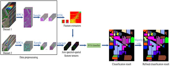
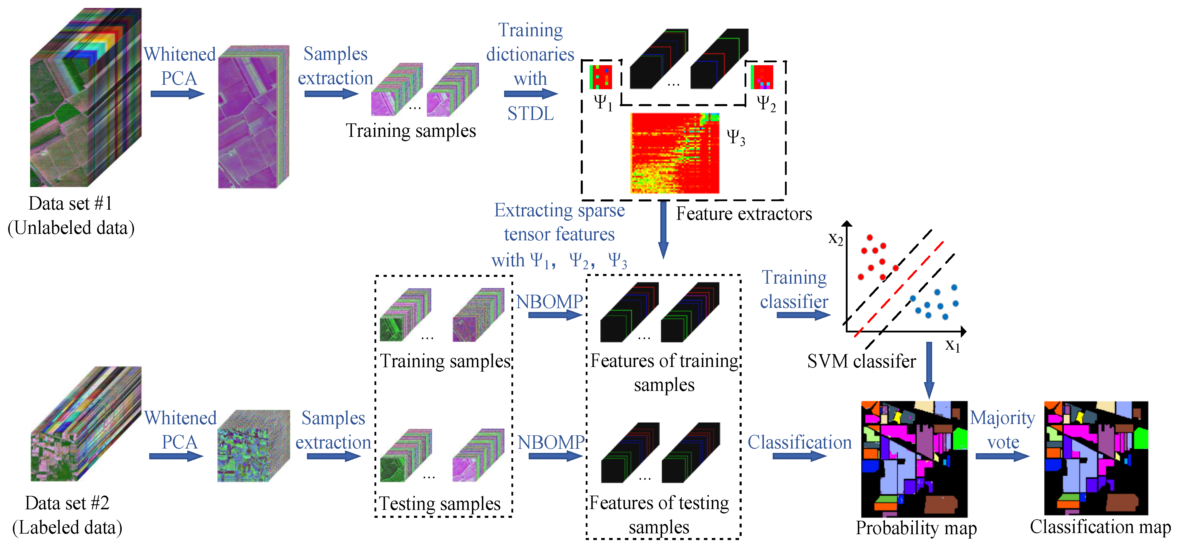
In this section, we describe the proposed TDSL classification method detailedly. Figure 1 shows the flow chart of TDSLMV, which includes three main steps: training feature extractors on the unlabeled data set #1, extracting features and classification for data set #2, and refining the classification results with the majority vote. For training feature extractors, we propose the STDL algorithm. Therefore, we introduce the STDL algorithm, first. Then, we describe the whole proposed classification methods, including TDSL and TDSLMV.

3.1. The Sparse Tensor-Based Dictionary Learning Algorithm

In the proposed classification method, we use the STDL to obtain feature extractors from unlabeled data set #1. The STDL trains three dictionaries for the order of three sample tensors, and it initializes dictionaries with TKD and updates dictionaries based on K-HOSVD [64,65]. The three dictionaries used in STDL correspond to two spatial dimensions and one spectral dimension, respectively, and when combined, the three dictionaries correspond to 3-D tensors. Therefore, the three dictionaries can be used to extract spectral-spatial feature tensors for 3-D HSI data.

In this paper, the HSI sample set is denoted as $\underline{X}\in {\mathbb{R}}^{n_1\times n_2\times n_3\times N}$, where $n_1$ and $n_2$ are the spatial sizes of the HSI samples, $n_3$ is the spectral size, and N is the number of samples.

We initialize the three dictionaries with the TKD of all training samples. For the ith sample ${\underline{X}}_i=\underline{X}(:,:,:,i)\in {\mathbb{R}}^{n_1\times n_2\times n_3}$, the TKD is denoted by:

$${\underline{X}}_i={\underline{C}}^{\left(i\right)}{\times }_1{A}_1^{\left(i\right)}{\times }_2{A}_2^{\left(i\right)}{\times }_3{A}_3^{\left(i\right)},$$

(9)

where $A_1^{\left(i\right)}\in {\mathbb{R}}^{n_1\times n_1}$, $A_2^{\left(i\right)}\in {\mathbb{R}}^{n_2\times n_2}$, $A_3^{\left(i\right)}\in {\mathbb{R}}^{n_3\times n_3}$, and ${\underline{C}}^{\left(i\right)}\in {\mathbb{R}}^{n_1\times n_2\times n_3}$. Then the dictionaries ${\mathrm{\Psi }}_1\in {\mathbb{R}}^{n_1\times n_1}$, ${\mathrm{\Psi }}_2\in {\mathbb{R}}^{n_2\times n_2}$, and ${\mathrm{\Psi }}_3\in {\mathbb{R}}^{n_3\times n_3}$ are obtained by:

$${\mathrm{\Psi }}_1=\sum _{i=1}^N{A}_1^{\left(i\right)},{\mathrm{\Psi }}_2=\sum _{i=1}^N{A}_2^{\left(i\right)},{\mathrm{\Psi }}_3=\sum _{i=1}^N{A}_3^{\left(i\right)}$$

(10)

The initial dictionaries are obtained after normalization:

$${\mathit{\psi }}_1^{j_1}={\displaystyle \frac{{\mathit{\psi }}_1^{j_1}}{\parallel {\mathit{\psi }}_1^{j_1}{\parallel }_F}},{\mathit{\psi }}_2^{j_2}={\displaystyle \frac{{\mathit{\psi }}_2^{j_2}}{\parallel {\mathit{\psi }}_2^{j_2}{\parallel }_F}},{\mathit{\psi }}_3^{j_1}={\displaystyle \frac{{\mathit{\psi }}_3^{j_1}}{\parallel {\mathit{\psi }}_3^{j_1}{\parallel }_F}},$$

(11)

where ${\mathit{\psi }}_1^{j_1}$ is the $j_1$th atom of ${\mathrm{\Psi }}_1$, (i.e., the $j_1$th column of ${\mathrm{\Psi }}_1$), $j_1=1,2,\dots ,n_1$ is the index of the atom, ${\mathit{\psi }}_2^{j_2}$ is the $j_2$th atom of ${\mathrm{\Psi }}_2$, $j_2=1,2,\dots ,n_2$, ${\mathit{\psi }}_3^{j_3}$ is the $j_3$th atom of ${\mathrm{\Psi }}_3$, and $j_3=1,2,\dots ,n_3$.

The dictionary learning algorithm solves the following optimization problem:

$$\begin{array}{cc}\hfill & \underset{{\mathrm{\Psi }}_1,{\mathrm{\Psi }}_2,{\mathrm{\Psi }}_2,\underline{Y}}{min}{\parallel \underline{X}-\underline{Y}{\times }_1{\mathrm{\Psi }}_1{\times }_2{\mathrm{\Psi }}_2{\times }_3{\mathrm{\Psi }}_3\parallel }_F^2,\hfill \\ \hfill & \mathrm{s}.\mathrm{t}.\parallel \underline{Y}{(:,:,:,i)\parallel }_0\le k,i=1,2,\dots ,N,\hfill \end{array}$$

(12)

where $\underline{Y}\in {\mathbb{R}}^{n_1\times n_2\times n_3\times N}$ is the sparse representation coefficient tensor, and k is the maximum number of non-zero elements in $\underline{Y}(:,:,:,i)$.

We solve Equation (12) by alternately performing the sparse representation and the update of dictionaries. First, we estimate the sparse representation coefficient tensor $\underline{Y}$ via the N-way block orthogonal matching pursuit (NBOMP) algorithm [67] with initial dictionaries. Then, we update dictionaries alternately, and we update one of the three dictionaries with the others fixed, i.e., update ${\mathrm{\Psi }}_1$ with ${\mathrm{\Psi }}_2$, ${\mathrm{\Psi }}_3$ fixed.

First, we update the dictionary ${\mathrm{\Psi }}_1$ atom by atom. When updating the $j_1$th atom of ${\mathrm{\Psi }}_1$, we first find the samples, which are sparsely represented by the $j_1$th atom. The indexes of these samples are obtained by inequation:

$$\parallel \underline{Y}(j_1,:,:,i){\parallel }_F^2>0.$$

(13)

The index set ${\mathcal{I}}_1$ contains all the i satisfied Equation (13). Thus, the sample subset $\underline{\tilde{X}}$ contains all the samples represented by the $j_1$th atom, which is denoted by:

$$\underline{\tilde{X}}=\underline{X}(:,:,:,{\mathcal{I}}_1).$$

(14)

Similarly, the corresponding sparse representation coefficient tensor is denoted as:

$$\underline{\tilde{Y}}=\underline{Y}(:,:,:,{\mathcal{I}}_1).$$

(15)

Then, the temporary dictionary ${\tilde{\mathrm{\Psi }}}_1$, which is the dictionary ${\mathrm{\Psi }}_1$ without the jth atom, is denoted by:

$${\mathrm{\Psi }}_1(:,j_1)=\mathbf{0}.$$

(16)

Next, we definite that:

$${\underline{R}}_{j_1}=\underline{\tilde{X}}-\underline{\tilde{Y}}{\times }_1{\tilde{\mathrm{\Psi }}}_1{\times }_2{\mathrm{\Psi }}_2{\times }_3{\mathrm{\Psi }}_3.$$

(17)

We carry out the HOSVD [63,66] for ${\underline{R}}_{j_1}$, which is represented as:

$${\underline{R}}_{j_1}\approx \lambda ·u_1\circ u_2\circ u_3\circ w.$$

(18)

Hence, the current atom is updated by:

$${\mathit{\psi }}_1^{j_1}={\displaystyle \frac{u_1}{\parallel u_1{\parallel }_F}},$$

(19)

$${\underline{\tilde{Y}}}_{j_1}{\times }_2{\mathrm{\Psi }}_2{\times }_3{\mathrm{\Psi }}_3=\lambda ·{\parallel u_1\parallel }_F·u_2\circ u_3\circ w,$$

(20)

where ${\underline{\tilde{Y}}}_{j_1}=\underline{Y}(j_1,:,:,{\mathcal{I}}_1)$. We update subtensor ${\underline{\tilde{Y}}}_{j_1}$ by solve Equation (20) with least square (LS).

After updating the dictionary ${\mathrm{\Psi }}_1$ and the corresponding sparse representation coefficients, we update ${\mathrm{\Psi }}_2$, ${\mathrm{\Psi }}_3$ seriatim. The procedures are similar to the previous description. Now the update steps of the dictionary ${\mathrm{\Psi }}_2$ corresponding to Equation (19), Equation (20) become:

$${\mathit{\psi }}_2^{j_2}={\displaystyle \frac{u_2}{\parallel u_2{\parallel }_F}},$$

(21)

$${\underline{\tilde{Y}}}_{j_2}{\times }_1{\mathrm{\Psi }}_1{\times }_3{\mathrm{\Psi }}_3=\lambda ·{\parallel u_2\parallel }_F·u_1\circ u_3\circ w,$$

(22)

where ${\underline{\tilde{Y}}}_{j_2}=\underline{Y}(:,j_2,:,{\mathcal{I}}_2)$. The index set ${\mathcal{I}}_2$ satisfies $\parallel \underline{Y}(:,j_2,:,i){\parallel }_F^2>0$. After updating every ${\mathit{\psi }}_2^{j_2}$ and ${\underline{\tilde{Y}}}_{j_2}$, we update the dictionary ${\mathrm{\Psi }}_3$. The update steps become:

$${\mathit{\psi }}_3^{j_3}={\displaystyle \frac{u_3}{\parallel u_3{\parallel }_F}},$$

(23)

$${\underline{\tilde{Y}}}_{j_3}{\times }_1{\mathrm{\Psi }}_1{\times }_2{\mathrm{\Psi }}_2=\lambda ·{\parallel u_3\parallel }_F·u_1\circ u_2\circ w,$$

(24)

where ${\underline{\tilde{Y}}}_{j_3}=\underline{Y}(:,:,j_3,{\mathcal{I}}_3)$. The index set ${\mathcal{I}}_3$ satisfies $\parallel \underline{Y}(:,:,j_3,i){\parallel }_F^2>0$.

The overall procedure of STDL is summarized in Algorithm 1.

Algorithm 1 The STDL Algorithm

Require: $\underline{X}\in {\mathbb{R}}^{n_1\times n_2\times n_3\times N}$, the maximum number of non-zero elements k, the maximum number of iterations $iter$, $t=0$.   1: Decompose every sample tensor $\underline{X}(:,:,:,i)$ with TKD by Equation (9);   2: Compute dictionaries ${\mathrm{\Psi }}_1,{\mathrm{\Psi }}_2,{\mathrm{\Psi }}_3$ by Equation (10), and normalize every dictionary by Equation (11) to obtain the initial dictionaries ${\mathrm{\Psi }}_1,{\mathrm{\Psi }}_2,{\mathrm{\Psi }}_3$;   3: while  $t\le iter$do   4:  Fix ${\mathrm{\Psi }}_1$, ${\mathrm{\Psi }}_2$, ${\mathrm{\Psi }}_3$, and solve Equation (12) via NBOMP [67] to obtain $\underline{Y}$;   5:  for every atom ${\mathit{\psi }}_1^{j_1}$ of ${\mathrm{\Psi }}_1$, $j_1=1$ to $n_1$ do   6:   ${\mathcal{I}}_1=[⌀]$;   7:   Find the index set ${\mathcal{I}}_1$ which contains all the i satisfied Equation (13);   8:   ${\mathrm{\Psi }}_1(:,j_1)=\mathbf{0}$, $\underline{\tilde{X}}=\underline{X}(:,:,:,{\mathcal{I}}_1)$, $\underline{\tilde{Y}}=\underline{Y}(:,:,:,{\mathcal{I}}_1)$;   9:   ${\underline{R}}_{j_1}=\underline{\tilde{X}}-\underline{\tilde{Y}}{\times }_1{\mathrm{\Psi }}_1{\times }_2{\mathrm{\Psi }}_2{\times }_3{\mathrm{\Psi }}_3$; 10:   Do HOSVD [63,66] for ${\underline{R}}_{j_1}\approx \lambda ·u_1\circ u_2\circ u_3\circ w$; 11:   Update ${\mathit{\psi }}_1^{j_1}$, ${\underline{\tilde{Y}}}_{j_1}{\times }_2{\mathrm{\Psi }}_2{\times }_3{\mathrm{\Psi }}_3$ using Equations (19) and (20), and calculate ${\underline{\tilde{Y}}}_{j_1}$ by LS; 12:  end for 13:  for every atom ${\mathit{\psi }}_2^{j_2}$ of ${\mathrm{\Psi }}_2$, $j_2=1$ to $n_2$ do 14:   ${\mathcal{I}}_2=[⌀]$; 15:   Find the index set ${\mathcal{I}}_2$ which contains all the i satisfied $\parallel \underline{Y}(:,j_2,:,i){\parallel }_F^2>0$; 16:   ${\mathrm{\Psi }}_2(:,j_2)=\mathbf{0}$, $\underline{\tilde{X}}=\underline{X}(:,:,:,{\mathcal{I}}_2)$, $\underline{\tilde{Y}}=\underline{Y}(:,:,:,{\mathcal{I}}_2)$; 17:   ${\underline{R}}_{j_2}=\underline{\tilde{X}}-\underline{\tilde{Y}}{\times }_1{\mathrm{\Psi }}_1{\times }_2{\mathrm{\Psi }}_2{\times }_3{\mathrm{\Psi }}_3$; 18:   Do HOSVD [63,66] for ${\underline{R}}_{j_2}\approx \lambda ·u_1\circ u_2\circ u_3\circ w$; 19:   Update ${\mathit{\psi }}_2^{j_2}$, ${\underline{\tilde{Y}}}_{j_2}{\times }_1{\mathrm{\Psi }}_1{\times }_3{\mathrm{\Psi }}_3$ using Equations (21) and (22), and calculate ${\underline{\tilde{Y}}}_{j_2}$ by LS; 20:  end for 21:  for every atom ${\mathit{\psi }}_3^{j_3}$ of ${\mathrm{\Psi }}_3$, $j_3=1$ to $n_3$do 22:   ${\mathcal{I}}_3=[⌀]$; 23:   Find the index set ${\mathcal{I}}_3$ which contains all the i satisfied $\parallel \underline{Y}(:,:,j_3,i){\parallel }_F^2>0$; 24:   ${\mathrm{\Psi }}_3(:,j_3)=\mathbf{0}$, $\underline{\tilde{X}}=\underline{X}(:,:,:,{\mathcal{I}}_3)$, $\underline{\tilde{Y}}=\underline{Y}(:,:,:,{\mathcal{I}}_3)$; 25:   ${\underline{R}}_{j_3}=\underline{\tilde{X}}-\underline{\tilde{Y}}{\times }_1{\mathrm{\Psi }}_1{\times }_2{\mathrm{\Psi }}_2{\times }_3{\mathrm{\Psi }}_3$; 26:   Do HOSVD [63,66] for ${\underline{R}}_{j_3}\approx \lambda ·u_1\circ u_2\circ u_3\circ w$; 27:   Update ${\mathit{\psi }}_3^{j_3}$, ${\underline{\tilde{Y}}}_{j_3}{\times }_1{\mathrm{\Psi }}_1{\times }_2{\mathrm{\Psi }}_2$ using Equations (23) and (24), and calculate ${\underline{\tilde{Y}}}_{j_3}$ by LS; 28:  end for 29:  $t=t+1$; 30: end while Ensure: ${\mathrm{\Psi }}_1,{\mathrm{\Psi }}_2,{\mathrm{\Psi }}_3$.

3.2. The Proposed Classification Methods

The proposed classification method TDSLMV for HSI is illustrated in Figure 1, and

Table 1. Definitions of symbols used in the proposed TDSLMV.

Symbol	Definition	Size
${\underline{Z}}_1$	the original data of data set #1	$n_1\times m_1\times B_1$
${\underline{Z}}_2$	the original data of data set #2	$n_2\times m_2\times B_2$
P	the spatial size of a sample patch	$1\times 1$
B	the number of principal components retained by PCA	$1\times 1$
$N_1$	the number of unlabeled training samples from data set #1	$1\times 1$
${\underline{X}}_1$	the unlabeled training data with samples extracted from data set #1 after PCA	$P\times P\times B\times N_1$
$N_2^{tr}$	the number of labeled training samples from data set #2	$1\times 1$
${\underline{X}}_2^{tr}$	the labeled training data with samples extracted from data set #2 after PCA	$P\times P\times B\times N_2^{tr}$
$N_2^{ts}$	the number of testing samples from data set #2	$1\times 1$
${\underline{X}}_2^{ts}$	the testing data with samples extracted from data set #2 after PCA	$P\times P\times B\times N_2^{ts}$
${\mathrm{\Psi }}_1,{\mathrm{\Psi }}_2,{\mathrm{\Psi }}_3$	the dictionaries which used as the feature extractors	$P\times P,P\times P,B\times B$
${\underline{Y}}_2^{tr}$	the feature tensor of the labeled training data ${\underline{X}}_2^{tr}$	$P\times P\times B\times N_2^{tr}$
${\underline{Y}}_2^{ts}$	the feature tensor of the testing data ${\underline{X}}_2^{ts}$	$P\times P\times B\times N_2^{ts}$
${\mu }_1$	the sparsity level parameter in tensor dictionary learning, i.e., the process of training feature extractors	$1\times 1$
${\mu }_2$	the sparsity level parameter in sparse representation, i.e., the process of extracting features	$1\times 1$
W	the window size in the majority vote	$1\times 1$

details the symbols used in the proposed TDSLMV. Moreover, the classification method TDSL consists of several steps: data preprocessing, training feature extractors, extracting joint spectral-spatial tensor features, training classifier, and classification. Furthermore, we add the majority vote to refine the classification results of TDSL, i.e., the proposed TDSLMV method.

Before training feature extractors and extracting features, the two data sets are both preprocessed with the same procedures. Whitened PCA (WPCA) is used to reduce the spectral dimensions of the two data sets, first. Redundancy exists in the spectral information of HSI, WPCA is applied to the spectral dimension to reduce the redundancy. Furthermore, WPCA can reduce the complexity of models. The new spectral dimensions of the two data sets are the same after WPCA, even though they are different before. The original data set #1 is denoted as ${\underline{Z}}_1\in {\mathbb{R}}^{n_1\times m_1\times B_1}$, $n_1$ and $m_1$ specify the spatial size, and $B_1$ is the number of spectral bands. We perform mode-3 matricization on ${\underline{Z}}_1$ to obtain a $B_1\times n_1{m}_1$ matrix $Z_1$. Then the WPCA of data set #1 is:

$$R=D^{-\frac{1}{2}}{E}^T{Z}_1,$$

(25)

where $R$ is the whitened matrix, $E$ consists of eigenvectors of the covariance matrix $Z_1{Z}_1^T$, and the corresponding eigenvalues of $E$ consist in a diagonal matrix $D$. Next, we reshape the matrix $R$ back to a $n_1\times m_1\times B$ tensor, B is the number of new spectral dimensions. The WPCA of data set #2 is similar to the previous procedures. Then the values of the two data sets are normalized to be 0 to 1, to reduce the luminance variance. We randomly extract sample patches of size $P\times P\times B$ from data set #1, denoted as ${\underline{X}}_1$. We extract the same size sample patches at every position with annotation from data set #2. All the samples are split into training set ${\underline{X}}_2^{tr}$ and testing set ${\underline{X}}_2^{ts}$ randomly.

Next, we perform STDL on unlabeled samples ${\underline{X}}_1$ from data set #1 to obtain the feature extractors ${\mathrm{\Psi }}_1$, ${\mathrm{\Psi }}_2$, ${\mathrm{\Psi }}_3$. The optimization problem is:

$$\begin{array}{cc}\hfill & \underset{{\mathrm{\Psi }}_1,{\mathrm{\Psi }}_2,{\mathrm{\Psi }}_2,{\underline{Y}}_1}{min}{\parallel {\underline{X}}_1-{\underline{Y}}_1{\times }_1{\mathrm{\Psi }}_1{\times }_2{\mathrm{\Psi }}_2{\times }_3{\mathrm{\Psi }}_3\parallel }_F^2,\hfill \\ \hfill & \mathrm{s}.\mathrm{t}.\parallel {\underline{Y}}_1{(:,:,:,i)\parallel }_0\le {\mu }_1·P^2·B,i=1,2,\dots ,N_1,\hfill \end{array}$$

(26)

where ${\mu }_1$ is the sparsity level, $N_1$ is the number of samples in ${\underline{X}}_1$.

Subsequently, we extract tensor features with ${\mathrm{\Psi }}_1$, ${\mathrm{\Psi }}_2$, ${\mathrm{\Psi }}_3$ on data set #2. The feature tensor ${\underline{Y}}_2^{tr}$ of the labeled training set ${\underline{X}}_2^{tr}$ is obtained via NBOMP [67],

$$\begin{array}{cc}\hfill & arg\underset{{\underline{Y}}_2^{tr}}{min}{\parallel {\underline{X}}_2^{tr}-{\underline{Y}}_2^{tr}{\times }_1{\mathrm{\Psi }}_1{\times }_2{\mathrm{\Psi }}_2{\times }_3{\mathrm{\Psi }}_3\parallel }_F^2,\hfill \\ \hfill & \mathrm{s}.\mathrm{t}.\parallel {\underline{Y}}_2^{tr}{(:,:,:,i)\parallel }_0\le {\mu }_2·P^2·B,i=1,2,\dots ,N_2^{tr},\hfill \end{array}$$

(27)

where ${\mu }_2$ is the sparsity level in sparse representation, $N_2^{tr}$ is the number of training samples from data set #2. Then, we vectorize the feature tensor of every sample. This amounts to mode-4 matricization on ${\underline{Y}}_2^{tr}$. Therefore, the input of the training SVM model is $Y_{2\left(4\right)}^{tr}$ with the shape of $N_2^{tr}\times P^{2}B$. The feature tensor ${\underline{Y}}_2^{tr}$ of the labeled training set affects the classifier performance directly. The quality of features and the number of features in the feature tensor both affect the performance of the classifier. The quality of features is determined directly by the feature extractors, i.e., the three dictionaries, and indirectly affected by the sparsity level parameter ${\mu }_1$. The number of features is determined by the sparsity level parameter ${\mu }_2$.

Once we obtain the SVM model, we can perform the classification procedures. When we classify the testing set ${\underline{X}}_2^{ts}$, we extract the corresponding tensor features first. We solve:

$$\begin{array}{cc}\hfill & arg\underset{{\underline{Y}}_2^{ts}}{min}{\parallel {\underline{X}}_2^{ts}-{\underline{Y}}_2^{ts}{\times }_1{\mathrm{\Psi }}_1{\times }_2{\mathrm{\Psi }}_2{\times }_3{\mathrm{\Psi }}_3\parallel }_F^2,\hfill \\ \hfill & \mathrm{s}.\mathrm{t}.\parallel {\underline{Y}}_2^{ts}{(:,:,:,i)\parallel }_0\le {\mu }_2·P^2·B,i=1,2,\dots ,N_2^{ts},\hfill \end{array}$$

(28)

to obtain the feature tensor ${\underline{Y}}_2^{ts}$ via NBOMP [67], where $N_2^{ts}$ is the number of testing samples from data set #2. Then, the input of the SVM model is the mode-4 matricization of ${\underline{Y}}_2^{ts}$. The output labels of the SVM model composite a probability map.

The proposed TDSL classification method consists of all the previous procedures. Furthermore, we can utilize the spatial information in the classification map of TDSL to improve the classification results. We refine the classification map via the majority vote. First, we extract a $W\times W$ patch for every pixel in the probability classification map obtained by TDSL. Then, we count the number of occurrences of every class in the patch. We determine the final label for the center pixel by the most frequent class.

$$C=arg\underset{c=1,\dots ,M}{max}\sum _{w=1}^{W^2}f(L_w,c),$$

(29)

$$f(L_w,c)=\left\{\begin{array}{c}1,if{L}_w=c\hfill \\ 0,if{L}_w\ne c\hfill \end{array}\right.$$

(30)

where $f(L_w,c)$ is the function for counting the number of occurrences of every class, $L_w$ is the label of wth pixel in the patch, and M is the number of all classes in data set #2. TDSLMV includes all of the above procedures, and Algorithm 2 summarizes all the steps.

Algorithm 2 The TDSLMV Algorithm

Require: Unlabeled data set #1 ${\underline{Z}}_1\in {\mathbb{R}}^{n_1\times m_1\times B_1}$, labeled data set #2 {${\underline{Z}}_2\in {\mathbb{R}}^{n_2\times m_2\times B_2}$, $L\in {\mathbb{R}}^{n_2\times m_2}$}.   1: Perform WPCA on ${\underline{Z}}_1$ to reduce the spectral dimensions, preserve the first B principal components, obtain ${\underline{\tilde{Z}}}_1\in {\mathbb{R}}^{n_1\times m_1\times B}$;   2: Randomly extract sample patches form ${\underline{\tilde{Z}}}_1$, obtain training data ${\underline{X}}_1$;   3: Perform STDL on ${\underline{X}}_1$ to obtain the feature extractors ${\mathrm{\Psi }}_1$, ${\mathrm{\Psi }}_2$, ${\mathrm{\Psi }}_3$ by solving Equation (26);   4: Perform WPCA on ${\underline{Z}}_2$ to reduce the spectral dimensions, preserve the first B principal components, obtain ${\underline{\tilde{Z}}}_2\in {\mathbb{R}}^{n_2\times m_2\times B}$;   5: Randomly extract sample patches form ${\underline{\tilde{Z}}}_2$, obtain labeled training set {${\underline{X}}_2^{tr}$, $L^{tr}$} and testing set ${\underline{X}}_2^{ts}$;   6: Extract feature tensor ${\underline{Y}}_2^{tr}$ of the labeled training set ${\underline{X}}_2^{tr}$ with ${\mathrm{\Psi }}_1$, ${\mathrm{\Psi }}_2$, ${\mathrm{\Psi }}_3$ by solving Equation (27);   7: Perform mode-4 matricization on ${\underline{Y}}_2^{tr}$ to obtain $Y_{2\left(4\right)}^{tr}$;   8: Train SVM model with the input {$Y_{2\left(4\right)}^{tr}$, $L^{tr}$};   9: Extract feature tensor ${\underline{Y}}_2^{ts}$ of the testing set ${\underline{X}}_2^{ts}$ with ${\mathrm{\Psi }}_1$, ${\mathrm{\Psi }}_2$, ${\mathrm{\Psi }}_3$ by solving Equation (28); 10: Perform mode-4 matricization on ${\underline{Y}}_2^{ts}$ to obtain $Y_{2\left(4\right)}^{ts}$; 11: Predict labels ${\tilde{L}}^{ts}$ of $Y_{2\left(4\right)}^{ts}$ with SVM model and obtain probability map; 12: Perform majority vote on probability map by Equations (29) and (30), obtain the classification map and the final labels $L^{ts}$. Ensure: SVM model, $L^{ts}$, and classification map.

3.3. Hypothesis and Limitations

The assumption behind self-taught models is that the features they learn to extract are generalizable, i.e., they will work well across data sets if their underlying natural statistics are similar [8]. The majority vote works under the hypothesis that the pixels belong to the same class if they are neighbors. Therefore, if the real class of a pixel is different from its surrounding pixels, then the pixel will be misclassified after the majority vote.

3.4. Computational Complexity Analysis

For a given training HSI data set with N samples, the computational complexity of training tensor feature extractors is mainly dominated by the update of dictionaries using K-HOSVD, which requires $\mathcal{O}\left(2P^4{B}^2(kN+P^4{B}^2)\right)$[64], where P is the spatial size of each sample, B is the number of spectral bands, k is the number of nonzero coefficients in each feature tensor, and the computational complexity of extracting features is $\mathcal{O}(6k^4+(2k+3)P^{2}B)$ [67].

4. Experimental Results and Analysis

In this section, we perform a series of experiments to evaluate our proposed classification methods. We utilize four widely used HSI benchmark data sets available on the website (http://www.ehu.eus/ccwintco/index.php?title=Hyperspectral_Remote_Sensing_Scenes (accessed on 25 July 2022)): the Salinas, the Indian Pines, the Pavia Center, and the Pavia University. The Salinas and the Pavia Center are used as unlabeled data sets (i.e., data set #1), the Indian Pines and the Pavia University are used as labeled data sets (i.e., data set #2). We perform experiments to demonstrate the proposed methods are effective for cross-scene and cross-sensor HSI classification. When data set #1 is the Salinas, we denote the proposed methods as TDSL-S and TDSLMV-S. When data set #1 is the Pavia Center, we denote the proposed methods as TDSL-P and TDSLMV-P.

Table 2. Definitions of abbreviations of the proposed methods in the experiments.

Abbreviation	Definition
TDSL	the proposed tensor-based dictionary self-taught learning classification method
TDSLMV	the TDSL followed by the majority vote
TDSL-S, TDSLMV-S	the data set #1 is Salinas, i.e., training feature extractors on Salinas
TDSL-P, TDSLMV-P	the data set #1 is Pavia Center, i.e., training feature extractors on Pavia Center

summarizes the abbreviations of the proposed methods. Furthermore, we apply the trained feature extractor model to a complex dataset Houston2013 (The data were provided by Prof. N. Yokoya from the University of Tokyo and RIKEN AIP) to demonstrate the advantages of the proposed methods in terms of applications. The feature extractor model and parameters are trained on the four aforementioned datasets, and we just retrain the SVM model on the Houston2013 data.

We compare our methods with several state-of-the-art methods: the SVM applied to spectral data [17], the SVM applied to contextual data (CSVM) [50], the spectral dictionary learning (SDL) [12], the simultaneous orthogonal matching pursuit (SOMP) [14], the spatial-aware dictionary learning (SADL) [13], the generalized tensor regression (GTR) [58], HybridSN [22], ASTDL-CNN [61] and SpectralFormer [32]. Among these methods, SVM, CSVM, SDL, and SADL belong to SVM-based methods. Simultaneously, SDL, SADL, SOMP, and ASTDL-CNN are sparse representation methods. HybridSN, ASTDL-CNN, and SpectralFormer belong to neural network methods. The proposed TDSL extracts features by sparse representation and classifies features with SVM, thus we compare it with both SVM-based methods and sparse representation methods. To demonstrate the effectiveness of feature extractors trained from other unlabeled data, we compare TDSL with SVM. CSVM is an improved SVM method. To demonstrate the effectiveness of dictionary learning in TDSL, we compare it with SDL and SADL. SDL is a spectral-based method, and SADL incorporates spectral information with spatial information. SOMP is a sparse representation method without the SVM classifier. It is worth comparing our methods with GTR because GTR utilizes tensor technology and it is necessary to compare our methods with neural network methods and our previous works. The codes of SVM, CSVM, SDL, SOMP, and SADL are available on the website (http://ssp.dml.ir/research/sadl/ (accessed on 7 May 2020)), the codes of GTR are available on the website (https://github.com/liuofficial/GTR (accessed on 25 July 2022)), the codes of HybridSN are available on the website (https://github.com/MVGopi/HybridSN (accessed on 25 July 2022)), and the codes of SpectralFormer are available on the website (https://github.com/danfenghong/IEEE_TGRS_SpectralFormer (accessed on 12 August 2022)).

For our proposed methods, the new number of spectral bands B is set to 50 for all experiments [60]. Ref. [60] demonstrates when B is larger than 40, the information preserved by PCA is sufficient to achieve high classification accuracy. The size of the extracted samples is set to $7\times 7\times 50$ (i.e., P is set to 7, which is the same as in [32]). Ref. [65] demonstrates the K-HOSVD can achieve convergence in about 5 iterations. Therefore, the maximum number of iterations for updating dictionaries in Algorithm 1 is set to 10 to guarantee convergence. Ref. [67] states when tolerance $\epsilon =0.01$, a sparse representation is correctly recovered. Moreover, the higher precision required, the smaller tolerance and more training time are needed. In our method, the tolerance $\epsilon$ in the NBOMP algorithm is set as $0.02$. The SVM used in the proposed methods is performed by using the radial basis function (RBF) kernel. In SVM, RBF-kernel parameter $\sigma$ and regularization parameter C can be optimally determined by five-fold cross-validation on the training set in the range of $\sigma =[2^{-8},2^{-7},\dots ,2^8]$ and $C=[2^{-8},2^{-7},\dots ,2^8]$.

The proposed methods implement tensor-based manipulation via the MATLAB Tensor Toolbox [68]. The SVM in all SVM-based methods is performed by the LIBSVM toolbox [69]. All the methods except the neural network methods are implemented in MATLAB 2017b on a 64-b octa-core CPU 2.60-GHz processor with 8-GB RAM. HybridSN, ASTDL-CNN, and SpectralFormer are performed in Python 3.6 with the library of Pytorch 1.3. Furthermore, we evaluate the classification results by three wildly used metrics, the overall accuracy (OA), the average accuracy (AA), and the Kappa coefficient (Kappa). The OA is the proportion of correctly classified samples to the overall samples in the testing set, the AA is the mean value of each category’s accuracies, and Kappa is calculated by weighting the measured accuracies [7].

4.1. Data Sets Description

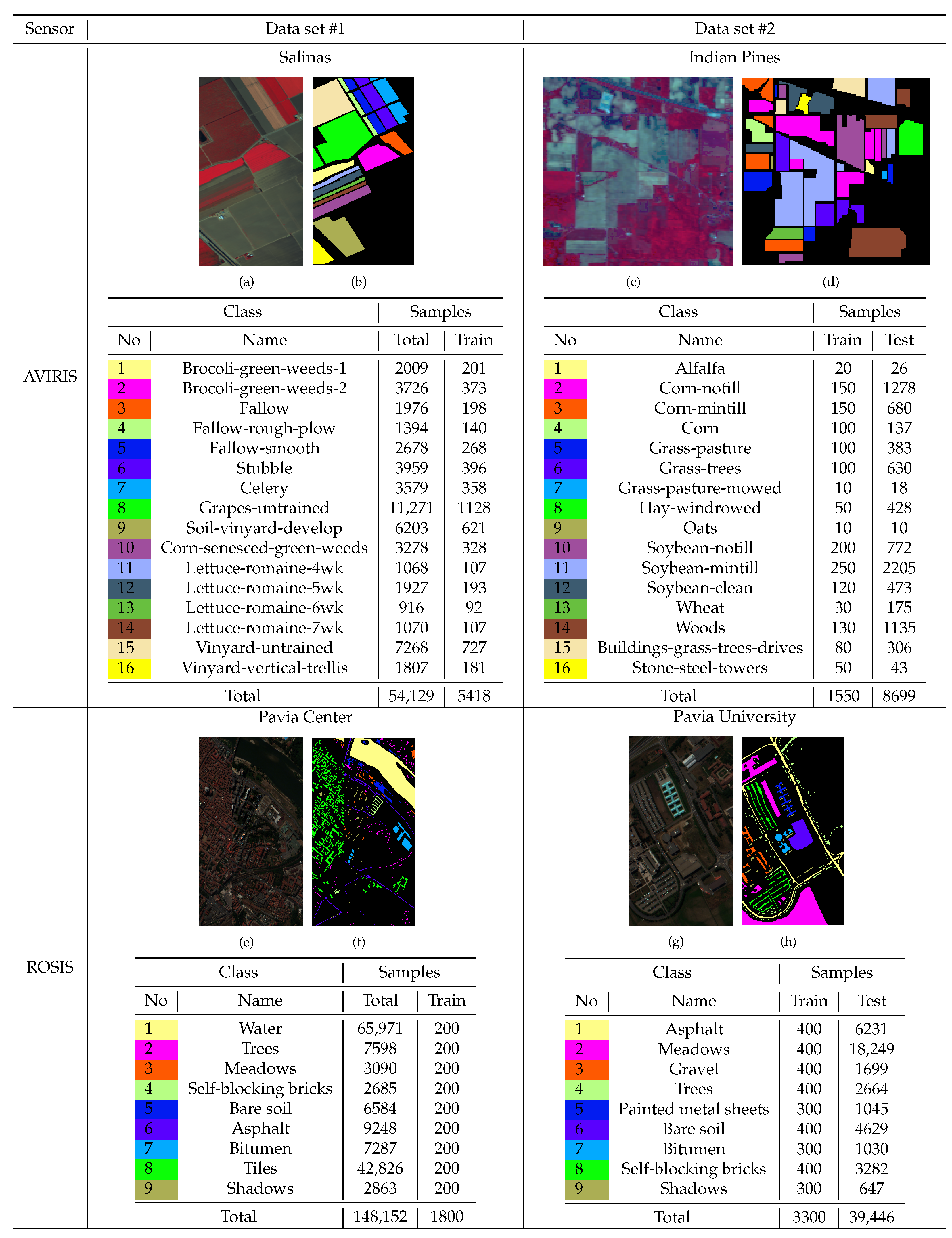
The five representative HSI data sets used in this paper are briefly described as follows. Figure 2 shows the composite three-band false-color maps, the ground truth maps, and the details of the samples for Salinas, Pavia Center, Indian Pines, and Pavia University.

Table 3. Information of the Houston2013 dataset, with the number of training and testing samples.

Class No.	Class Name	Training	Testing
1	Healthy Grass	198	1053
2	Stressed Grass	190	1064
3	Synthetic Grass	192	505
4	Tree	188	1056
5	Soil	186	1056
6	Water	182	143
7	Residential	196	1072
8	Commercial	191	1053
9	Road	193	1059
10	Highway	191	1036
11	Railway	181	1054
12	Parking Lot1	192	1041
13	Parking Lot2	184	285
14	Tennis Court	181	247
15	Runing Track	187	473
	Total	2832	12,197

shows the information of the Houston2013 dataset.

We first introduce the data sets used as unlabeled data sets, i.e., data set #1.

(1) Salinas: This data set is collected by the Airborne Visible/Infrared Imaging Spectrometer (AVIRIS) sensor over Salinas Valley in California. The HSI consists of $512\times 217$ pixels with a spatial resolution of $3.7$ meters per pixel. The AVIRIS gathers 224 bands in the wavelength range 0.4–2.5 $\mathsf{\mu }$m, whereas we remove 20 bands, which are noisy or cover the water absorption region. Therefore, we use 204 spectral bands in the experiments. The ground truth of Salinas contains 16 classes, including bare soils, vegetables, and vineyard fields. The details of these classes are displayed in the corresponding table in Figure 2. We use $10\%$ samples of every class as the unlabeled samples to train feature extractors.

(2) Pavia Center: This data set is gathered by the Reflective Optics Spectrometer (ROSIS) over Pavia in northern Italy. The HSI consists of $1096\times 715$ pixels, and the spatial resolution is $1.3$ meters per pixel. The ROSIS sensor captures 115 bands with a spectral range of 0.43–0.86 $\mathsf{\mu }$m. The number of spectral bands is 102 after removing the noisy bands. The ground truth contains 9 classes, and the detailed information of every class is shown in the corresponding table in Figure 2. We randomly choose 200 samples from every class as the unlabeled samples to train feature extractors.

Next, we introduce the data sets used as labeled training data and testing data, i.e., data set #2.

(1) Indian Pines: This data set is collected by the AVIRIS sensor over the Indian Pines in Northwestern Indiana. The scene consists of $145\times 145$ pixels, and the spatial resolution is 20 meters per pixel. We preserve 200 bands after removing noisy bands in the experiments. The ground truth contains 16 classes, including agriculture, forest, and natural perennial vegetation. The details of the information, including the name of every class, the numbers of training samples, and the numbers of testing samples, are displayed in the corresponding table in Figure 2. The number of training samples accounts for about $15\%$ of the total samples with annotation.

(2) Pavia University: This data set is gathered by the ROSIS sensor surrounding the university of Pavia. The image consists of $610\times 340$ pixels, and the number of spectral bands for the experiments is 103. The spatial resolution is the same as the Pavia Center. The ground truth contains 9 classes, and the classes are different from the classes of Pavia Center. The details of every class are displayed in the corresponding table in Figure 2. We randomly choose 300 or 400 samples from every class as the labeled training samples, and the total proportion is less than $1\%$.

Finally, we introduce the Houston2013 dataset. This data set is gathered by the ITRES CASI-1500 sensor over the campus of the University of Houston and its neighboring rural areas in the USA. The image consists of $349\times 1905$ pixels and 144 bands with a spectral range of 0.364–1.046 $\mathsf{\mu }$m. The ground truth contains 15 classes. The details of every class are displayed in Table 3, whose background colors indicate different classes of land-covers, and the numbers of training samples are set according to [32].

4.2. Influence of the Sparsity Levels

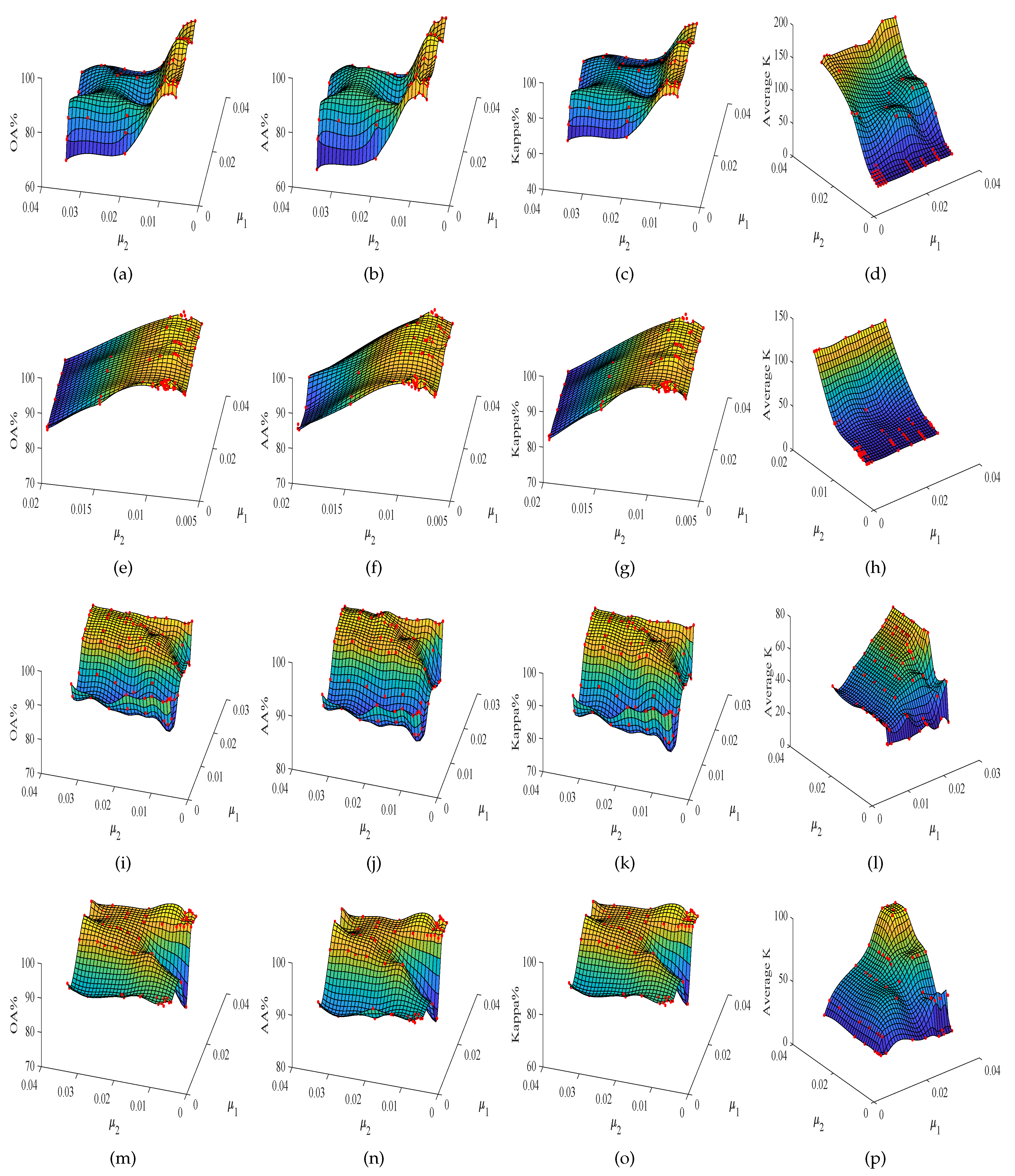
In the proposed TDSL classification method, there are two sparsity level parameters, one is in Equation (26) to train feature extractors on data set #1 via the STDL algorithm, and the other one is in Equations (27) and (28) to extract tensor features on data set #2 via the NBOMP algorithm. Equations (26)–(28) show that the sparsity level parameters decide the number of nonzero coefficients in feature tensors, and the number of nonzero coefficients in feature tensors is also related to the size of the input data. The number of nonzero coefficients in feature tensors affects the classification accuracy. Therefore, the sparsity level parameters are selected according to the size of the input data and ensure that the number of nonzero coefficients in each feature tensor is enough. We suggest that the number of nonzero coefficients in each feature tensor should be over 20. In this study, we analyze the impacts of the two sparsity level parameters ${\mu }_1$ and ${\mu }_2$ according to the experiment results of methods: TDSL-S on the Indian Pines data set, TDSL-P on the Indian Pines, TDSL-S on Pavia University, and TDSL-P on Pavia University. The numbers of training samples in the two data sets and the numbers of testing samples in data set #2 are set as Figure 2. The results are displayed in Figure 3. In Figure 3, the red dots are the actual experiment results, and the three-dimensional surfaces are fitted according to these red dots. The surfaces can clearly show the influence of the sparsity level parameters on classification results. We evaluate the sparsity level parameters by the OA, AA, and Kappa. Furthermore, the actual number of nonzero coefficients in the sparse feature tensor for every sample in data set #2 is denoted as K, and the average K for the whole data set #2 is also displayed in Figure 3.

Figure 3 shows the variation of classification accuracies with the two sparsity level parameters ${\mu }_1$ and ${\mu }_2$. Moreover, ${\mu }_1$, ${\mu }_2$ together decide the actual numbers of nonzero coefficients in tensor features K, and affect the classification results. Furthermore, for different data set #2, the variation tendency is different. The first row and the second row from top to bottom indicate the results on Indian Pines, i.e., data set #2 is the Indian Pines in the experiments. The third row and the fourth row indicate the results on Pavia University, i.e., data set #2 is the Pavia University in the experiments. The first row and the second row have a similar variation tendency, the third row and the fourth row also have a similar variation tendency. Figure 3a–h show that OA, AA, and Kappa of TDSL-S and TDSL-P on Indian Pines increase with the decrease in ${\mu }_2$, while K decreases with the decrease in ${\mu }_2$, when ${\mu }_1$ is fixed. Moreover, when ${\mu }_2$ is fixed, with the change of ${\mu }_1$, the OA, AA, Kappa, and K remain the same or fluctuate within a certain range. Figure 3i–p show that the OA, AA, and Kappa of TDSL-S and TDSL-P on Pavia University increase first and then fluctuate within a certain range, with the increase in ${\mu }_1$ when ${\mu }_2$ is fixed. Moreover, when ${\mu }_1$ is fixed, the OA, AA, Kappa increase first and then fluctuate within a certain range with the increase in ${\mu }_2$.

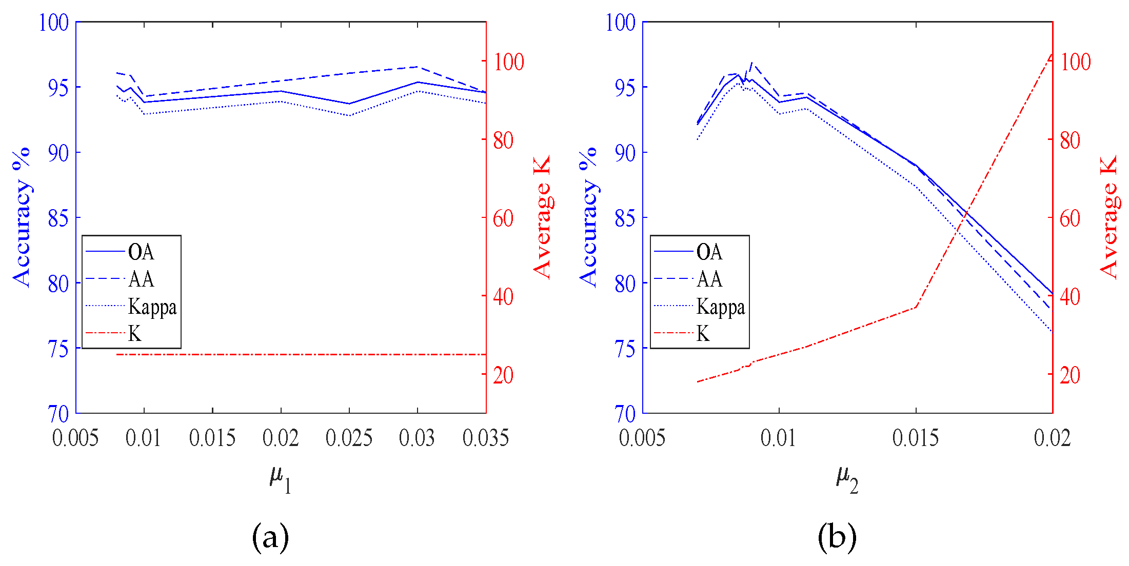
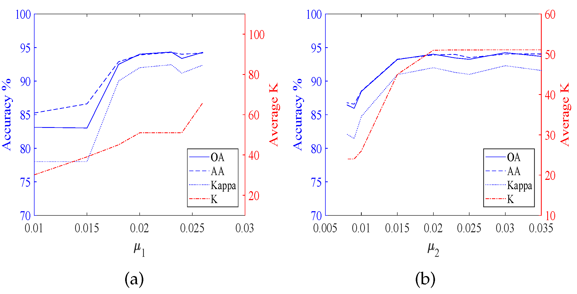
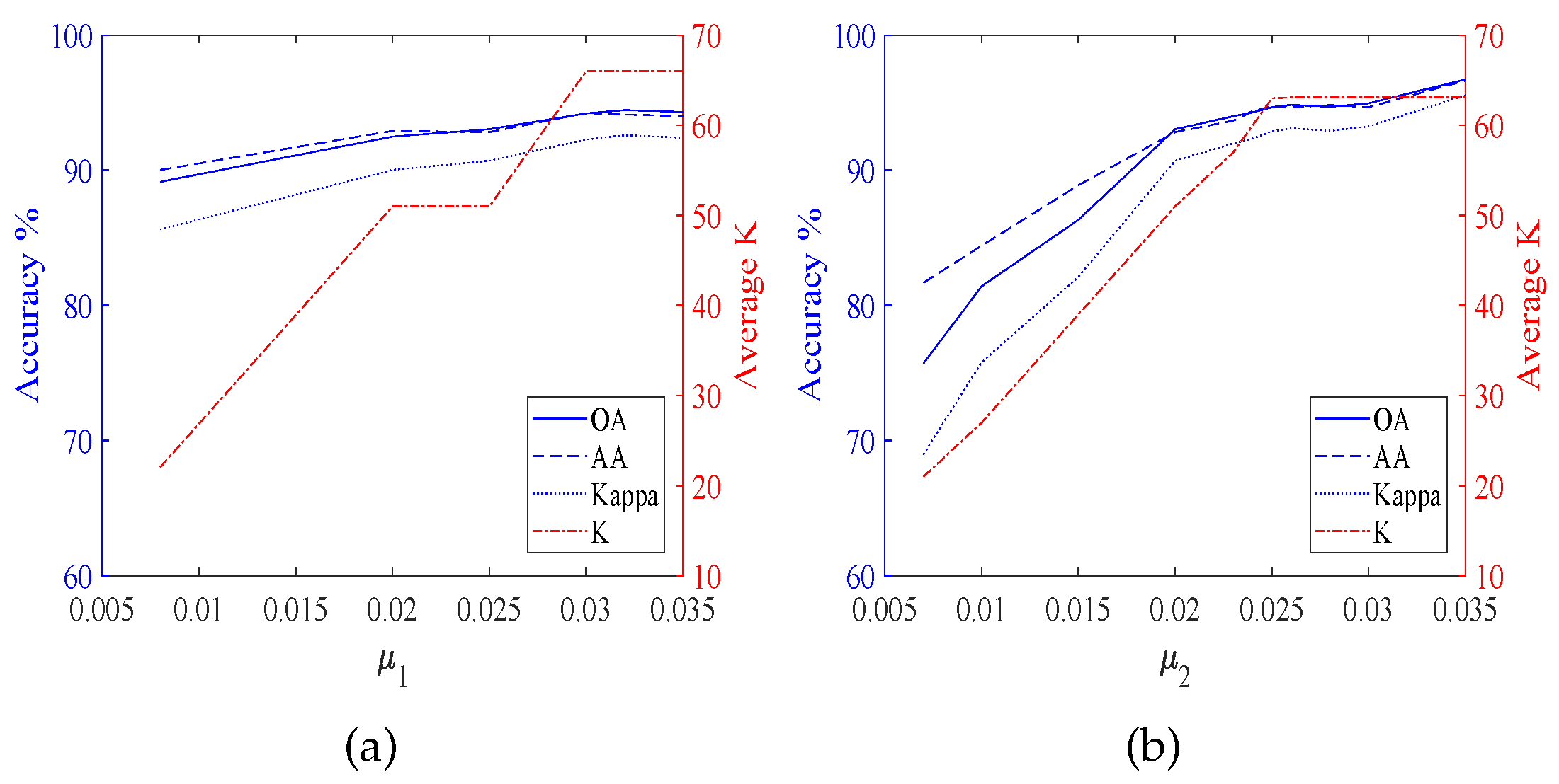
According to Figure 3, it is obvious that the classification accuracies are affected by both ${\mu }_1$ and ${\mu }_2$. Furthermore, Figure 4, Figure 5, Figure 6 and Figure 7 display the classification accuracies and K are affected by ${\mu }_1$ or ${\mu }_2$ when the other one is fixed. Figure 4 shows the results of TDSL-S on Indian Pines, and Figure 5 shows the results of TDSL-P on Indian Pines. Figure 4a and Figure 5a show that K remains the same and accuracies fluctuate within a certain range when ${\mu }_2$ is fixed. Figure 4b and Figure 5b shows that accuracies increase first and then decrease with the increase in ${\mu }_2$ when ${\mu }_1$ is fixed and K increases with the increase in ${\mu }_2$. Figure 6 shows the results of TDSL-S on Pavia University, and Figure 7 shows the results of TDSL-P on Pavia University. Figure 6a and Figure 7a show that accuracies increase first and then fluctuate within a certain range with the increase in ${\mu }_1$ when ${\mu }_2$ is fixed and K increases step by step with the increase in ${\mu }_1$. Figure 6b and Figure 7b show that accuracies increase first and then fluctuate within a certain range with the increase in ${\mu }_2$ when ${\mu }_1$ is fixed. Moreover, K increases first and then remains the same with the increase in ${\mu }_2$ when ${\mu }_1$ is fixed.

For all the experiments, the classification accuracies are related to the average K. The classification accuracies increase with the increase in the average K, at first. It is because the average K represents the number of features in the sparse feature tensor. When the number of features is small, the information represented by these features is not enough to classify. Whereas, when the average K is larger than a certain value, the classification accuracies fluctuate in a certain range or decrease. It is because when the number of features is large enough, the information is enough for classification. The fluctuation is due to noise and the SVM model. However, if there are too many features, the classifier will be difficult to classify. The average K is related to the two sparsity level parameters ${\mu }_1$, ${\mu }_2$, and the error of the least-squares optimization problem Equations (26)–(28). For different data set #2, the satisfied optimization termination conditions of NBOMP are different. For Indian Pines, when the number of nonzero coefficients gets to ${\mu }_2·p^2·B$, the optimization of sparse representation stops. Therefore, in Figure 3d,h, Figure 4b and Figure 5b, the K increases with the increase in ${\mu }_2$. Whereas the influence of ${\mu }_1$ on K is small. For Pavia University, the error of sparse representation satisfies the conditions for loop termination, before the number of nonzero coefficients gets to ${\mu }_2·p^2·B$. In this case, the ${\mu }_1$ decides the maximum of K, and the ${\mu }_2$ decides the actual number of K. When the ${\mu }_2$ is smaller than ${\mu }_1$, the average K increases with the increase in ${\mu }_2$ first but when the ${\mu }_2$ gets to ${\mu }_1$, the average K keeps the same, despite the ${\mu }_2$ continuing to increase. This phenomenon is obvious in Figure 3l,p, Figure 6b and Figure 7b.

According to these experiment results, we determine the parameters. The two sparsity level parameters in the experiments for the two data sets are set as in

Table 4. The sparsity level parameters for the proposed methods on the two data sets.

Data Set #2	Indian Pines		Pavia University
Method	TDSL-S	TDSL-P	TDSL-S	TDSL-P
${\mu }_1$	0.008	0.035	0.026	0.032
${\mu }_2$	0.01	0.0087	0.008	0.0089

.

4.3. Influence of the Majority Vote

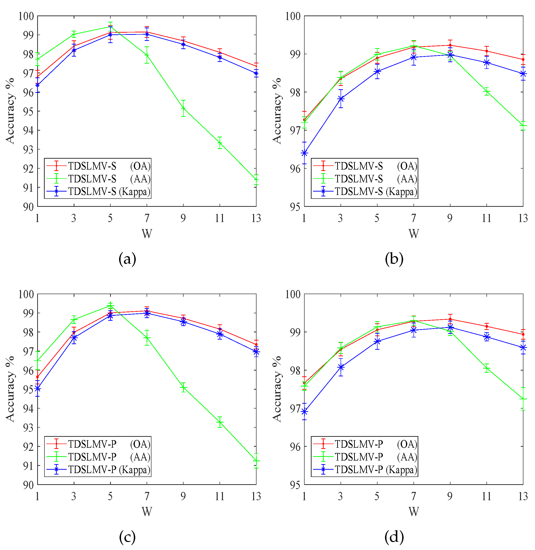
After the proposed TDSL gets a probability classification map, we can use the majority vote to refine the classification results. This is denoted as TDSLMV. The majority vote utilizes the spatial information in the classification map. We vote in a $W\times W$ window, and the parameter W influences the refined results. The results on the two data sets #2, (i.e., the Indian Pines, and the Pavia University) are displayed in Figure 8.

It is obvious that the majority vote can refine the classification accuracies to a certain extent, in Figure 8. When the W equals to 1, the TDSLMV becomes TDSL. Figure 8 shows the classification accuracies (the OA, AA, and Kappa) increase with the increase in W first, and then the accuracies decrease with the increase of W. In Figure 8a,c, maximum accuracies are achieved when $W=5$. In Figure 8b,d, maximum accuracies are achieved when $W=7$. The majority vote works under the assumption that the pixels belong to the same class if they are neighbors. Whereas, when W is larger than a certain value, the pixels in the window are more likely to belong to different classes. Therefore, when W is larger than a certain value, the accuracies decrease. For different data sets, the most appropriate W is different. From Figure 8, we can easily obtain that the most appropriate W for Indian Pines is 5, and for Pavia University $W=7$.

4.4. Parameter Setting for the Comparison Methods

In this work, we compare the proposed methods with nine state-of-the-art HSI classification methods, including:

1.

SVM [17] is applied to the spectral bands of every pixel in the HSI. The kernel of the SVM is a polynomial kernel, and the optimal parameters (polynomial kernel degree d, and regularization parameter C) are obtained by five-fold cross-validation on the training set in the range of $d=[1,2,\dots ,10]$, and $C=[{10}^{-1},1,10,\dots ,{10}^7]$.

2.

CSVM [50] is SVM applied to the contextual data. The window width of the contextual data is set as 7. The kernel of SVM is a radial basis function (RBF) kernel, and the parameters (RBF-kernel parameter $\sigma$ and regularization parameter C) are also obtained by five-fold cross-validation on the training set in the range of $\sigma =[0.1,1,10,100]$, and $C=[{10}^{-1},1,10,\dots ,{10}^7]$.

3.

SDL [12] is a sparse dictionary learning method with spectral data. It utilizes dictionary learning to extract features and uses SVM to classify. We also use five-fold cross-validation to determine the parameters. The sparse regularization parameter ranges in $\{0.1,1,10,100\}$. The number of dictionary atoms is proportional to the number of training samples, the proportion is chosen from $\{\frac{1}{2},\frac{1}{4},\frac{1}{8},\frac{1}{16}\}$.

4.

SOMP [14] is a sparse representation method. The method incorporates contextual information into spectral data. The test samples are sparsely represented by the training samples and directly determined the labels according to the sparse representation. The parameters of SOMP are set as those in [14].

5.

SADL [13] method is a sparse dictionary learning method applied to the data incorporating spectral and contextual information, and the sparse coefficients are classified by SVM. The patch size parameter is set as $7\times 7$, and the other parameters of SADL are set as the same as those in [13].

6.

The generalized tensor regression (GTR) [58] method extends the ridge regression with multivariate labels to the tensorial version. GTR takes advantage of tensorial representation with the nonnegative constraint. The spatial size is set as $7\times 7$, and the other parameters are set as the same as those in [58].

7.

HybridSN [22] is a CNN method, which assembles 3-D CNN and 2-D CNN. The epoch is set as 10, the batch size is set as 20, and the learning rate is set as $0.001$ and the numbers of PCA components are set as the same as in [22].

8.

ASTDL-CNN [61] is the tensor-based method and CNN-based method, the parameters are set as the same as reported in [61].

9.

SpectralFormer [32] is a transformer-based backbone network, which is focused on spectrometric characteristics. The pixel-wise SpectralFormer is compared, and the parameters are set as the same as those in [32].

4.5. Comparisons with Different Classification Methods

We evaluate the proposed methods by comparing them with the aforementioned methods on two wildly used data sets (the Indian Pines, and the Pavia University). Moreover, the two data sets correspond to data set #2 in our proposed methods. When we train feature extractors on the data set Salinas (i.e., data set #1 is the salinas), the methods are denoted with ‘-S’, and when data set #1 is the Pavia Center, the methods are denoted with ‘-P’. We evaluate the proposed TDSL and TDSLMV at the same time. To demonstrate that the proposed methods are effective in the cross-scene classification, we perform TDSL-S, TDSLMV-S on the Indian Pines data, and perform TDSL-P, TDSLMV-P on the Pavia data, where data set #1 and data set #2 are gathered by the same sensor but over different scenes. Furthermore, to demonstrate that the proposed methods can work in the cross-scene and cross-sensor classification, we perform TDSL-S, TDSLMV-S on Pavia University, and perform TDSL-P, TDSLMV-P on the Indian Pines, where the data set #1 and data set #2 are gathered by different sensors over difference scenes.

We perform the experiments with randomly extracted samples ten times for every method, and the numbers of training samples and testing samples are as shown in Figure 2. The classification results for the Indian Pines data are reported in Table 5. We report the results in the form of ‘mean value ± standard deviation’. Table 5 shows that SVM and SDL obtain poor results since they just utilize spectral data. SpectralFormer obtains better results than SVM and SDL, although the input of SpectralFormer is also spectral data. It demonstrates the superiority of neural network methods. CSVM gets better results than SVM, and SADL obtains better results than SDL, which demonstrates that contextual information is important for HSI classification. SOMP provides worse results than SADL, though they are both sparse representation methods applied to both spectral and contextual data. This implies that training dictionaries from training samples and classifying the corresponding sparse coefficients by SVM can improve the classification. Furthermore, SVM can not only give the classification results but also can extract further features from the sparse coefficients. GTR provides better results than other methods except for the proposed methods, this stresses that the tensor technology is more beneficial to the HSI classification. The results of HybridSN are better than SVM, CSVM, SDL, SOMP, SADL, and SpectralFormer, because HybridSN extracts spectral-spatial features by 3-D CNN and 2-D CNN. ASTDL-CNN obtains better results than HybridSN, because ASTDL can extract intrinsic tensor features, which are more conducive to classification. HybridSN and ASTDL-CNN are CNN-based methods and need more labeled data than GTR, therefore, the results of GTR are better than those of HybridSN and ASTDL-CNN. The results of TDSL-S are better than those of SVM, which demonstrates that the feature extractors learned from another unlabeled data set can extract discriminative features for classification. The results of TDSL-P demonstrate that the proposed method can provide very high classification accuracies even meeting the cross-scene and cross-sensor task. TDSLMV-S provides the best results in terms of the OA, AA, and Kappa. The OA of TDSLMV-S achieves as high as $99.13\%$, and even the OA of TDSLMV-P achieves as high as $98.99\%$ in cross-scene and cross-sensor classification tasks. Compared with GTR, the average OA of TDSLMV-S is improved by $2.48\%$. Furthermore, the standard deviations are small which means that the proposed methods are robust.

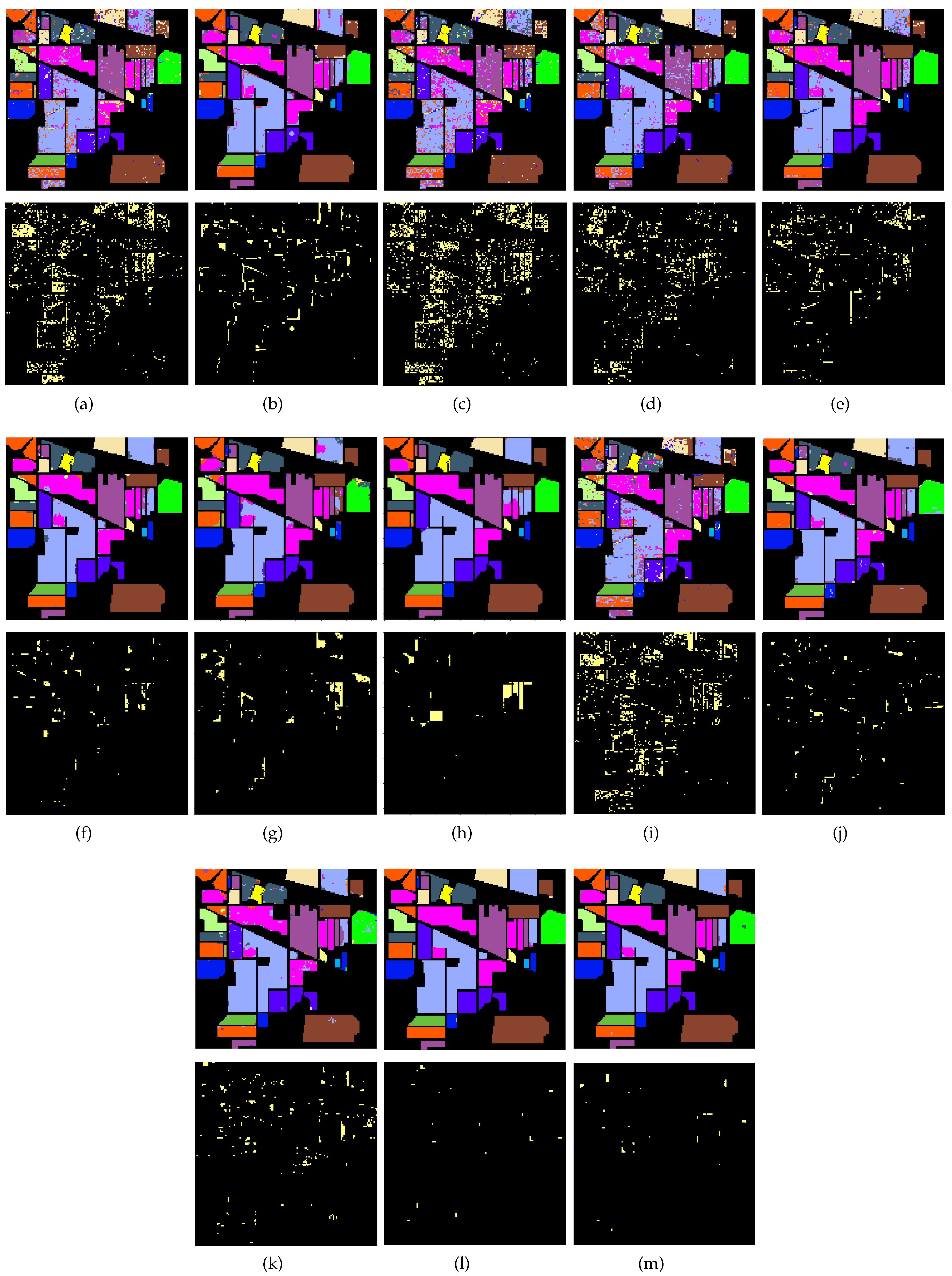
Figure 9 illustrates the classification maps obtained by the thirteen aforementioned methods for the Indian Pines. It can be easily observed that many isolated misclassified pixels appear in the classification maps of the spectral methods SVM, SDL, and SpectralFormer. From Figure 9b,d,e we can easily observe that the utilization of contextual information can effectively reduce the isolated misclassified pixels. From Figure 9g,h,j–m, we can observe that very few isolated misclassified pixels appear in the classification maps of the tensor-based methods (GTR, HybridSN, ASTDL-CNN, and our methods). However, the misclassified pixels are more likely to appear together in the classification maps for tensor-based methods. Especially, the misclassified pixels appear at the edges between two different homogenous regions. Figure 9g,h show that the misclassified pixels tend to appear in small homogenous regions. This is because the tensor samples may contain pixels belonging to different classes, especially when extracting samples at the edges between different homogenous regions. Figure 9l,m show that the majority vote can refine the classification, correcting most of the misclassified pixels in the large homogenous regions and at the edges of different homogenous regions. Therefore, the classification map of TDSLMV-S is the most similar to the ground truth map of the Indian Pines.

Table 5. Classification accuracies (Mean Value ± Standard Deviation %) of different methods for the Indian Pines data set, bold values indicate the best result for a row.

CLASS	SVM [17]	CSVM [50]	SDL [12]	SOMP [14]	SADL [13]	GTR [58]	HybridSN [22]	ASTDL-CNN [61]	SpectralFormer [32]	TDSL-S	TDSL-P	TDSLMV-S	TDSLMV-P
1	$87.69\pm 8.74$	$86.15\pm 11.78$	$86.83\pm 4.68$	$88.08\pm 4.23$	$95.77\pm 3.37$	$98.08\pm 2.03$	$98.56\pm 2.86$	$98.37\pm 1.01$	$89.74\pm 2.22$	$99.57\pm 0.92$	$93.70\pm 4.52$	$\mathbf{100}.\mathbf{00}\pm \mathbf{0}.\mathbf{00}$	$\mathbf{100}.\mathbf{00}\pm \mathbf{0}.\mathbf{00}$
2	$66.44\pm 2.26$	$85.23\pm 2.57$	$68.98\pm 4.08$	$73.75\pm 4.47$	$82.87\pm 2.32$	$92.59\pm 2.08$	$86.96\pm 8.96$	$80.54\pm 3.41$	$69.69\pm 4.37$	$94.47\pm 0.75$	$92.34\pm 1.68$	$\mathbf{98}.\mathbf{56}\pm \mathbf{0}.\mathbf{71}$	$97.46\pm 0.80$
3	$74.29\pm 2.82$	$92.90\pm 1.43$	$66.47\pm 3.64$	$70.07\pm 4.50$	$89.44\pm 2.25$	$96.56\pm 0.76$	$93.66\pm 2.41$	$\mathbf{99}.\mathbf{59}\pm \mathbf{0}.\mathbf{16}$	$76.86\pm 2.39$	$97.14\pm 0.79$	$96.29\pm 1.45$	$99.37\pm 0.54$	$99.40\pm 0.94$
4	$85.69\pm 1.67$	$98.61\pm 1.06$	$73.83\pm 5.43$	$94.23\pm 2.27$	$94.82\pm 2.24$	$99.93\pm 0.23$	$97.54\pm 3.70$	$\mathbf{100}.\mathbf{00}\pm \mathbf{0}.\mathbf{00}$	$86.37\pm 3.45$	$99.75\pm 0.67$	$98.90\pm 1.21$	$\mathbf{100}.\mathbf{00}\pm \mathbf{0}.\mathbf{00}$	$\mathbf{100}.\mathbf{00}\pm \mathbf{0}.\mathbf{00}$
5	$93.42\pm 1.28$	$96.19\pm 2.22$	$92.36\pm 1.98$	$94.49\pm 1.42$	$96.14\pm 1.16$	$97.18\pm 1.07$	$94.35\pm 3.79$	$96.01\pm 0.15$	$89.64\pm 3.95$	$97.72\pm 1.07$	$96.77\pm 1.56$	$\mathbf{99}.\mathbf{57}\pm \mathbf{0}.\mathbf{38}$	$99.15\pm 0.85$
6	$94.75\pm 1.38$	$97.68\pm 1.04$	$92.98\pm 1.91$	$97.59\pm 1.32$	$98.40\pm 1.40$	$99.60\pm 0.21$	$92.10\pm 5.85$	$99.78\pm 0.07$	$94.76\pm 3.30$	$98.93\pm 0.52$	$98.16\pm 0.71$	$\mathbf{99}.\mathbf{99}\pm \mathbf{0}.\mathbf{04}$	$99.96\pm 0.13$
7	$85.56\pm 11.97$	$96.67\pm 5.37$	$81.53\pm 12.02$	$82.22\pm 10.41$	$96.67\pm 2.87$	$\mathbf{100}.\mathbf{00}\pm \mathbf{0}.\mathbf{00}$	$94.44\pm 7.86$	$98.21\pm 1.91$	$92.59\pm 6.42$	$98.93\pm 3.39$	$\mathbf{100}.\mathbf{00}\pm \mathbf{0}.\mathbf{00}$	$99.64\pm 1.13$	$\mathbf{100}.\mathbf{00}\pm \mathbf{0}.\mathbf{00}$
8	$94.70\pm 2.22$	$95.75\pm 2.65$	$94.39\pm 1.68$	$99.02\pm 0.60$	$99.44\pm 0.83$	$99.98\pm 0.07$	$89.28\pm 10.54$	$\mathbf{100}.\mathbf{00}\pm \mathbf{0}.\mathbf{00}$	$95.79\pm 4.05$	$95.77\pm 3.31$	$89.50\pm 5.38$	$98.87\pm 2.33$	$98.72\pm 1.40$
9	$84.00\pm 9.17$	$89.00\pm 7.38$	$73.00\pm 21.11$	$79.00\pm 14.49$	$97.00\pm 6.75$	$\mathbf{100}.\mathbf{00}\pm \mathbf{0}.\mathbf{00}$	$93.75\pm 17.68$	$78.75\pm 14.08$	$\mathbf{100}.\mathbf{00}\pm \mathbf{0}.\mathbf{00}$	$99.00\pm 2.11$	$99.50\pm 1.58$	$99.50\pm 1.58$	$\mathbf{100}.\mathbf{00}\pm \mathbf{0}.\mathbf{00}$
10	$78.41\pm 1.92$	$92.24\pm 1.63$	$68.93\pm 3.08$	$79.02\pm 3.36$	$92.40\pm 1.31$	$97.23\pm 1.22$	$95.68\pm 2.59$	$94.83\pm 2.64$	$89.29\pm 5.14$	$96.99\pm 0.99$	$97.53\pm 0.38$	$99.31\pm 0.73$	$\mathbf{99}.\mathbf{68}\pm \mathbf{0}.\mathbf{39}$
11	$77.33\pm 2.26$	$91.44\pm 1.95$	$67.44\pm 1.30$	$90.44\pm 1.99$	$89.24\pm 1.49$	$95.11\pm 0.81$	$95.89\pm 3.16$	$97.20\pm 1.40$	$81.53\pm 1.79$	$95.70\pm 1.24$	$94.74\pm 1.41$	$\mathbf{98}.\mathbf{46}\pm \mathbf{1}.\mathbf{01}$	$98.40\pm 0.86$
12	$83.74\pm 1.92$	$90.44\pm 1.67$	$84.63\pm 3.81$	$75.22\pm 2.24$	$90.38\pm 1.89$	$96.15\pm 1.12$	$91.09\pm 2.57$	$98.33\pm 0.57$	$74.63\pm 7.21$	$94.64\pm 1.49$	$94.60\pm 1.66$	$98.55\pm 1.18$	$\mathbf{99}.\mathbf{39}\pm \mathbf{0}.\mathbf{53}$
13	$97.49\pm 1.28$	$94.57\pm 5.59$	$98.12\pm 1.37$	$98.23\pm 0.83$	$99.09\pm 0.90$	$98.97\pm 0.70$	$93.29\pm 4.71$	$\mathbf{99}.\mathbf{94}\pm \mathbf{0}.\mathbf{17}$	$98.10\pm 0.87$	$98.00\pm 1.46$	$94.68\pm 4.12$	$99.56\pm 0.284$	$98.88\pm 1.32$
14	$93.02\pm 2.04$	$95.54\pm 1.06$	$88.19\pm 2.07$	$97.79\pm 1.20$	$97.63\pm 0.71$	$99.57\pm 0.16$	$95.01\pm 3.41$	$98.97\pm 1.94$	$91.48\pm 3.63$	$99.25\pm 0.49$	$98.42\pm 0.44$	$99.88\pm 0.25$	$\mathbf{99}.\mathbf{89}\pm \mathbf{0}.\mathbf{15}$
15	$67.68\pm 3.38$	$96.27\pm 1.24$	$69.81\pm 4.41$	$95.16\pm 2.29$	$95.20\pm 2.08$	$98.43\pm 1.05$	$94.40\pm 4.58$	$99.38\pm 0.77$	$65.58\pm 10.69$	$99.25\pm 0.59$	$98.37\pm 1.14$	$\mathbf{99}.\mathbf{95}\pm \mathbf{0}.\mathbf{16}$	$99.77\pm 0.39$
16	$97.21\pm 1.74$	$95.12\pm 3.87$	$92.33\pm 4.66$	$99.77\pm 0.74$	$97.21\pm 2.40$	$\mathbf{100}.\mathbf{00}\pm \mathbf{0}.\mathbf{00}$	$98.26\pm 2.41$	$98.92\pm 0.00$	$95.35\pm 4.65$	$98.49\pm 0.91$	$99.14\pm 0.68$	$99.68\pm 0.52$	$99.25\pm 0.73$
OA	$81.16\pm 0.81$	$92.42\pm 0.70$	$76.38\pm 0.65$	$87.02\pm 0.58$	$91.80\pm 0.44$	$96.65\pm 0.32$	$93.28\pm 1.74$	$95.58\pm 0.82$	$83.04\pm 0.90$	$96.81\pm 0.34$	$95.63\pm 0.37$	$\mathbf{99}.\mathbf{13}\pm \mathbf{0}.\mathbf{37}$	$98.99\pm 0.23$
AA	$85.09\pm 1.40$	$93.36\pm 0.84$	$81.24\pm 1.53$	$88.38\pm 0.80$	$94.48\pm 0.63$	$98.09\pm 0.25$	$94.02\pm 1.32$	$96.18\pm 1.06$	$86.96\pm 0.33$	$97.73\pm 0.34$	$96.42\pm 0.64$	$\mathbf{99}.\mathbf{43}\pm \mathbf{0}.\mathbf{24}$	$99.37\pm 0.14$
Kappa	$78.47\pm 0.90$	$91.30\pm 0.79$	$73.02\pm 0.71$	$85.03\pm 0.67$	$90.61\pm 0.50$	$96.16\pm 0.37$	$92.27\pm 1.99$	$94.95\pm 0.94$	$80.59\pm 1.06$	$96.36\pm 0.39$	$95.02\pm 0.42$	$\mathbf{99}.\mathbf{01}\pm \mathbf{0}.\mathbf{42}$	$98.85\pm 0.26$

Table 5. Classification accuracies (Mean Value ± Standard Deviation %) of different methods for the Indian Pines data set, bold values indicate the best result for a row.

CLASS	SVM [17]	CSVM [50]	SDL [12]	SOMP [14]	SADL [13]	GTR [58]	HybridSN [22]	ASTDL-CNN [61]	SpectralFormer [32]	TDSL-S	TDSL-P	TDSLMV-S	TDSLMV-P
1	$87.69\pm 8.74$	$86.15\pm 11.78$	$86.83\pm 4.68$	$88.08\pm 4.23$	$95.77\pm 3.37$	$98.08\pm 2.03$	$98.56\pm 2.86$	$98.37\pm 1.01$	$89.74\pm 2.22$	$99.57\pm 0.92$	$93.70\pm 4.52$	$\mathbf{100}.\mathbf{00}\pm \mathbf{0}.\mathbf{00}$	$\mathbf{100}.\mathbf{00}\pm \mathbf{0}.\mathbf{00}$
2	$66.44\pm 2.26$	$85.23\pm 2.57$	$68.98\pm 4.08$	$73.75\pm 4.47$	$82.87\pm 2.32$	$92.59\pm 2.08$	$86.96\pm 8.96$	$80.54\pm 3.41$	$69.69\pm 4.37$	$94.47\pm 0.75$	$92.34\pm 1.68$	$\mathbf{98}.\mathbf{56}\pm \mathbf{0}.\mathbf{71}$	$97.46\pm 0.80$
3	$74.29\pm 2.82$	$92.90\pm 1.43$	$66.47\pm 3.64$	$70.07\pm 4.50$	$89.44\pm 2.25$	$96.56\pm 0.76$	$93.66\pm 2.41$	$\mathbf{99}.\mathbf{59}\pm \mathbf{0}.\mathbf{16}$	$76.86\pm 2.39$	$97.14\pm 0.79$	$96.29\pm 1.45$	$99.37\pm 0.54$	$99.40\pm 0.94$
4	$85.69\pm 1.67$	$98.61\pm 1.06$	$73.83\pm 5.43$	$94.23\pm 2.27$	$94.82\pm 2.24$	$99.93\pm 0.23$	$97.54\pm 3.70$	$\mathbf{100}.\mathbf{00}\pm \mathbf{0}.\mathbf{00}$	$86.37\pm 3.45$	$99.75\pm 0.67$	$98.90\pm 1.21$	$\mathbf{100}.\mathbf{00}\pm \mathbf{0}.\mathbf{00}$	$\mathbf{100}.\mathbf{00}\pm \mathbf{0}.\mathbf{00}$
5	$93.42\pm 1.28$	$96.19\pm 2.22$	$92.36\pm 1.98$	$94.49\pm 1.42$	$96.14\pm 1.16$	$97.18\pm 1.07$	$94.35\pm 3.79$	$96.01\pm 0.15$	$89.64\pm 3.95$	$97.72\pm 1.07$	$96.77\pm 1.56$	$\mathbf{99}.\mathbf{57}\pm \mathbf{0}.\mathbf{38}$	$99.15\pm 0.85$
6	$94.75\pm 1.38$	$97.68\pm 1.04$	$92.98\pm 1.91$	$97.59\pm 1.32$	$98.40\pm 1.40$	$99.60\pm 0.21$	$92.10\pm 5.85$	$99.78\pm 0.07$	$94.76\pm 3.30$	$98.93\pm 0.52$	$98.16\pm 0.71$	$\mathbf{99}.\mathbf{99}\pm \mathbf{0}.\mathbf{04}$	$99.96\pm 0.13$
7	$85.56\pm 11.97$	$96.67\pm 5.37$	$81.53\pm 12.02$	$82.22\pm 10.41$	$96.67\pm 2.87$	$\mathbf{100}.\mathbf{00}\pm \mathbf{0}.\mathbf{00}$	$94.44\pm 7.86$	$98.21\pm 1.91$	$92.59\pm 6.42$	$98.93\pm 3.39$	$\mathbf{100}.\mathbf{00}\pm \mathbf{0}.\mathbf{00}$	$99.64\pm 1.13$	$\mathbf{100}.\mathbf{00}\pm \mathbf{0}.\mathbf{00}$
8	$94.70\pm 2.22$	$95.75\pm 2.65$	$94.39\pm 1.68$	$99.02\pm 0.60$	$99.44\pm 0.83$	$99.98\pm 0.07$	$89.28\pm 10.54$	$\mathbf{100}.\mathbf{00}\pm \mathbf{0}.\mathbf{00}$	$95.79\pm 4.05$	$95.77\pm 3.31$	$89.50\pm 5.38$	$98.87\pm 2.33$	$98.72\pm 1.40$
9	$84.00\pm 9.17$	$89.00\pm 7.38$	$73.00\pm 21.11$	$79.00\pm 14.49$	$97.00\pm 6.75$	$\mathbf{100}.\mathbf{00}\pm \mathbf{0}.\mathbf{00}$	$93.75\pm 17.68$	$78.75\pm 14.08$	$\mathbf{100}.\mathbf{00}\pm \mathbf{0}.\mathbf{00}$	$99.00\pm 2.11$	$99.50\pm 1.58$	$99.50\pm 1.58$	$\mathbf{100}.\mathbf{00}\pm \mathbf{0}.\mathbf{00}$
10	$78.41\pm 1.92$	$92.24\pm 1.63$	$68.93\pm 3.08$	$79.02\pm 3.36$	$92.40\pm 1.31$	$97.23\pm 1.22$	$95.68\pm 2.59$	$94.83\pm 2.64$	$89.29\pm 5.14$	$96.99\pm 0.99$	$97.53\pm 0.38$	$99.31\pm 0.73$	$\mathbf{99}.\mathbf{68}\pm \mathbf{0}.\mathbf{39}$
11	$77.33\pm 2.26$	$91.44\pm 1.95$	$67.44\pm 1.30$	$90.44\pm 1.99$	$89.24\pm 1.49$	$95.11\pm 0.81$	$95.89\pm 3.16$	$97.20\pm 1.40$	$81.53\pm 1.79$	$95.70\pm 1.24$	$94.74\pm 1.41$	$\mathbf{98}.\mathbf{46}\pm \mathbf{1}.\mathbf{01}$	$98.40\pm 0.86$
12	$83.74\pm 1.92$	$90.44\pm 1.67$	$84.63\pm 3.81$	$75.22\pm 2.24$	$90.38\pm 1.89$	$96.15\pm 1.12$	$91.09\pm 2.57$	$98.33\pm 0.57$	$74.63\pm 7.21$	$94.64\pm 1.49$	$94.60\pm 1.66$	$98.55\pm 1.18$	$\mathbf{99}.\mathbf{39}\pm \mathbf{0}.\mathbf{53}$
13	$97.49\pm 1.28$	$94.57\pm 5.59$	$98.12\pm 1.37$	$98.23\pm 0.83$	$99.09\pm 0.90$	$98.97\pm 0.70$	$93.29\pm 4.71$	$\mathbf{99}.\mathbf{94}\pm \mathbf{0}.\mathbf{17}$	$98.10\pm 0.87$	$98.00\pm 1.46$	$94.68\pm 4.12$	$99.56\pm 0.284$	$98.88\pm 1.32$
14	$93.02\pm 2.04$	$95.54\pm 1.06$	$88.19\pm 2.07$	$97.79\pm 1.20$	$97.63\pm 0.71$	$99.57\pm 0.16$	$95.01\pm 3.41$	$98.97\pm 1.94$	$91.48\pm 3.63$	$99.25\pm 0.49$	$98.42\pm 0.44$	$99.88\pm 0.25$	$\mathbf{99}.\mathbf{89}\pm \mathbf{0}.\mathbf{15}$
15	$67.68\pm 3.38$	$96.27\pm 1.24$	$69.81\pm 4.41$	$95.16\pm 2.29$	$95.20\pm 2.08$	$98.43\pm 1.05$	$94.40\pm 4.58$	$99.38\pm 0.77$	$65.58\pm 10.69$	$99.25\pm 0.59$	$98.37\pm 1.14$	$\mathbf{99}.\mathbf{95}\pm \mathbf{0}.\mathbf{16}$	$99.77\pm 0.39$
16	$97.21\pm 1.74$	$95.12\pm 3.87$	$92.33\pm 4.66$	$99.77\pm 0.74$	$97.21\pm 2.40$	$\mathbf{100}.\mathbf{00}\pm \mathbf{0}.\mathbf{00}$	$98.26\pm 2.41$	$98.92\pm 0.00$	$95.35\pm 4.65$	$98.49\pm 0.91$	$99.14\pm 0.68$	$99.68\pm 0.52$	$99.25\pm 0.73$
OA	$81.16\pm 0.81$	$92.42\pm 0.70$	$76.38\pm 0.65$	$87.02\pm 0.58$	$91.80\pm 0.44$	$96.65\pm 0.32$	$93.28\pm 1.74$	$95.58\pm 0.82$	$83.04\pm 0.90$	$96.81\pm 0.34$	$95.63\pm 0.37$	$\mathbf{99}.\mathbf{13}\pm \mathbf{0}.\mathbf{37}$	$98.99\pm 0.23$
AA	$85.09\pm 1.40$	$93.36\pm 0.84$	$81.24\pm 1.53$	$88.38\pm 0.80$	$94.48\pm 0.63$	$98.09\pm 0.25$	$94.02\pm 1.32$	$96.18\pm 1.06$	$86.96\pm 0.33$	$97.73\pm 0.34$	$96.42\pm 0.64$	$\mathbf{99}.\mathbf{43}\pm \mathbf{0}.\mathbf{24}$	$99.37\pm 0.14$
Kappa	$78.47\pm 0.90$	$91.30\pm 0.79$	$73.02\pm 0.71$	$85.03\pm 0.67$	$90.61\pm 0.50$	$96.16\pm 0.37$	$92.27\pm 1.99$	$94.95\pm 0.94$	$80.59\pm 1.06$	$96.36\pm 0.39$	$95.02\pm 0.42$	$\mathbf{99}.\mathbf{01}\pm \mathbf{0}.\mathbf{42}$	$98.85\pm 0.26$

The classification results for Pavia University are reported in Table 6, and the corresponding classification maps are illustrated in Figure 10. The results of HybridSN and ASTDL-CNN are better than CSVM, SOMP, SADL, and GTR, and the results of SpectralFormer are better than SVM and SDL. It demonstrates that neural network-based methods can achieve better results when the labeled samples are enough. The results of TDSL-S are higher than the comparison methods, which means the proposed method is superior to the other methods even for the cross-scene and cross-sensor classification tasks. Moreover, TDSLMV-P provides the highest accuracies in terms of the OA, AA, and Kappa. The average OA of TDSLMV-P achieves $99.28\%$, which is very high in all methods for HSI classification. Even for the cross-scene and cross-sensor classification, the average OA of TDSLMV-S achieves as high as $99.21\%$. Compared with ASTDL-CNN, the average OA of TDSLMV-P is improved by $2.61\%$. Furthermore, the standard deviations of OA, AA, and Kappa, for our proposed methods (i.e., TDSL-S, TDSL-P, TDSLMV-S, TDSLMV-P) are smaller than those for the other methods. This further demonstrates the robustness of our methods.

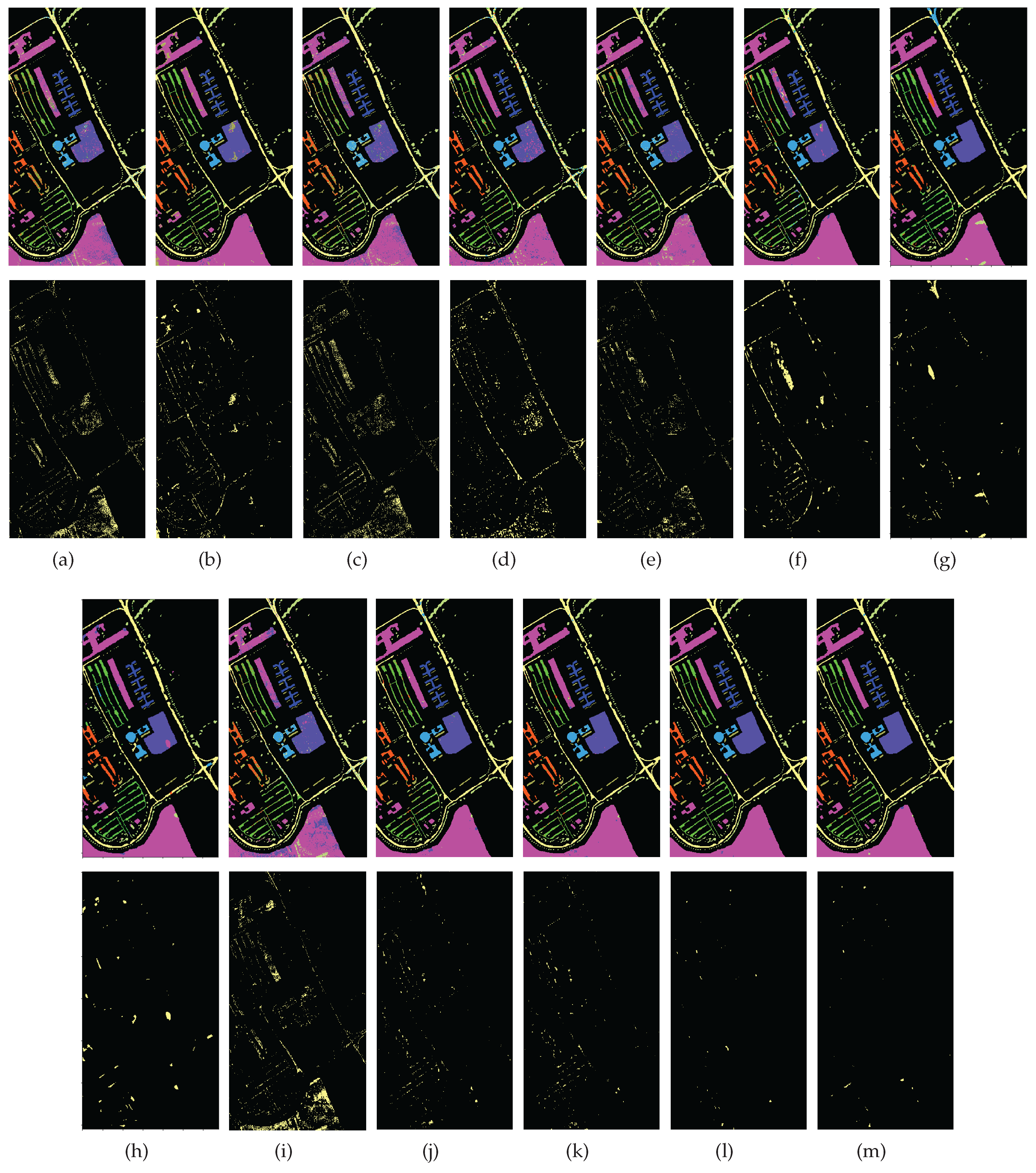
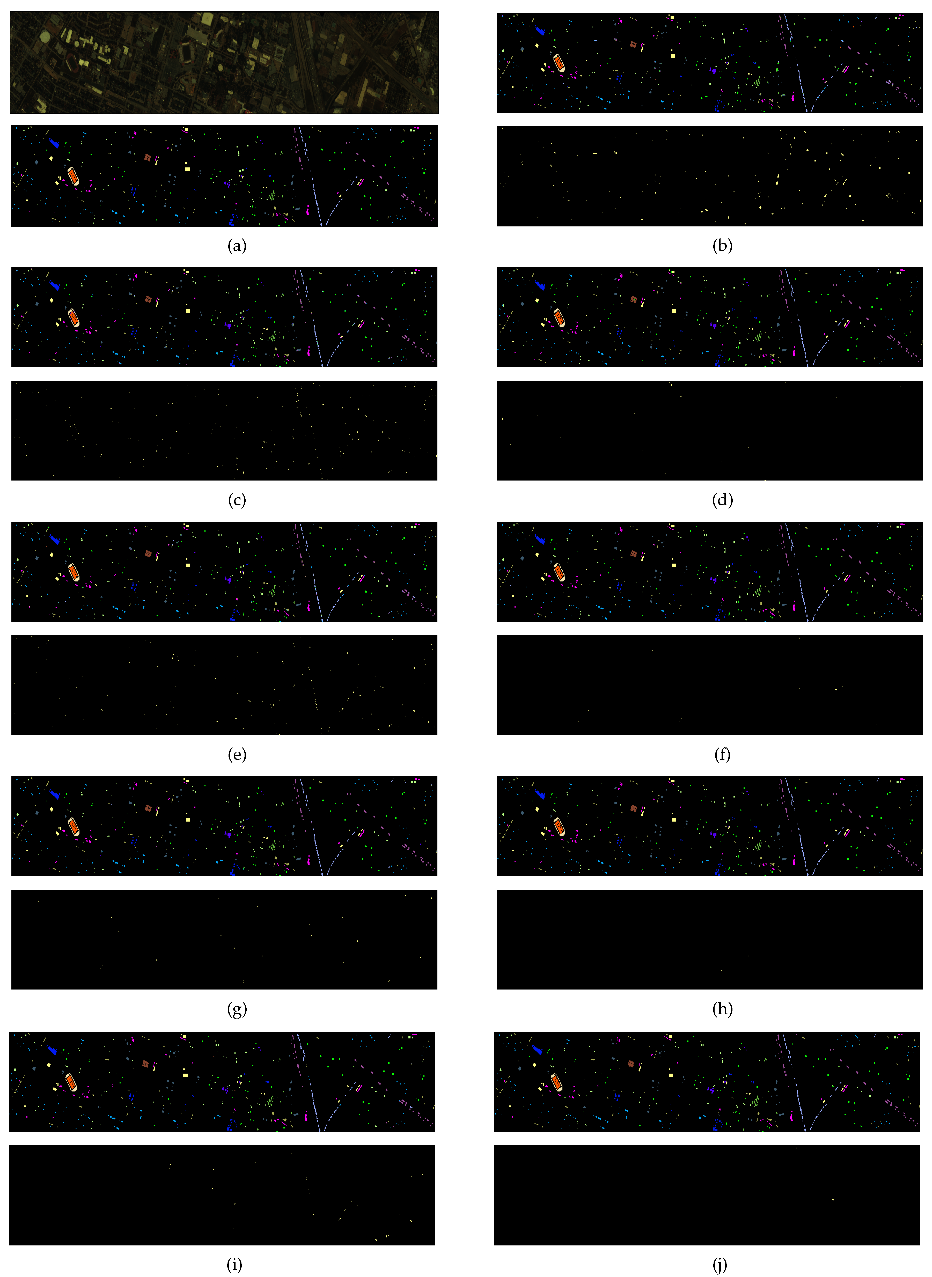
Figure 10 illustrates the classification maps and the corresponding error maps for the aforementioned methods. Unlike the Indian Pines, Pavia University consists of many small homogenous regions, which means that Pavia University contains more edge. Therefore, the performance of GTR on Pavia University data is worse than it on Indian Pines data. Figure 10a,c,i show that the misclassified pixels for spectral methods appear not only at the edges but also in the large homogenous regions. From Figure 10b,e, we can infer that the utilization of contextual information can reduce the misclassified pixels in large homogenous regions. Furthermore, the misclassified pixels for tensor-based methods mainly appear at the edges and in the small homogenous regions, which is observed from Figure 10f–h,j,k. However, Figure 10j,m show that the majority vote can also correct the misclassified pixels at edges and in the little homogenous regions.

Table 6. Classification accuracies (Mean Value ± Standard Deviation %) of different methods for the Pavia University data set, bold values indicate the best result for a row.

CLASS	SVM [17]	CSVM [50]	SDL [12]	SOMP [14]	SADL [13]	GTR [58]	HybridSN [22]	ASTDL-CNN [61]	SpectralFormer [32]	TDSL-S	TDSL-P	TDSLMV-S	TDSLMV-P
1	$84.01\pm 0.79$	$88.94\pm 1.33$	$89.09\pm 0.89$	$68.51\pm 1.11$	$88.78\pm 1.08$	$77.41\pm 1.18$	$92.33\pm 5.09$	$96.78\pm 1.67$	$87.56\pm 0.89$	$95.68\pm 0.75$	$96.81\pm 0.58$	$98.68\pm 0.41$	$\mathbf{99}.\mathbf{38}\pm \mathbf{0}.\mathbf{38}$
2	$87.16\pm 1.30$	$92.98\pm 0.77$	$84.95\pm 1.20$	$90.49\pm 1.12$	$93.26\pm 1.33$	$94.01\pm 1.70$	$94.67\pm 4.40$	$97.12\pm 1.73$	$83.01\pm 3.17$	$98.44\pm 0.40$	$98.49\pm 0.32$	$\mathbf{99}.\mathbf{42}\pm \mathbf{0}.\mathbf{30}$	$99.40\pm 0.30$
3	$77.85\pm 1.06$	$88.06\pm 1.60$	$78.23\pm 1.74$	$93.78\pm 0.91$	$88.97\pm 1.41$	$90.99\pm 1.77$	$91.97\pm 12.12$	$92.06\pm 2.52$	$83.68\pm 3.60$	$94.31\pm 0.80$	$95.66\pm 0.69$	$98.66\pm 0.94$	$\mathbf{99}.\mathbf{16}\pm \mathbf{0}.\mathbf{66}$
4	$97.09\pm 0.54$	$82.43\pm 1.58$	$94.88\pm 1.06$	$96.56\pm 0.56$	$97.64\pm 0.61$	$94.01\pm 0.68$	$94.99\pm 3.22$	$95.27\pm 2.41$	$92.91\pm 1.15$	$98.92\pm 0.35$	$98.94\pm 0.31$	$\mathbf{99}.\mathbf{22}\pm \mathbf{0}.\mathbf{29}$	$99.03\pm 0.35$
5	$99.91\pm 0.05$	$90.00\pm 1.51$	$99.84\pm 0.14$	$\mathbf{100}.\mathbf{00}\pm \mathbf{0}.\mathbf{00}$	$99.81\pm 0.16$	$\mathbf{100}.\mathbf{00}\pm \mathbf{0}.\mathbf{00}$	$99.42\pm 0.99$	$99.99\pm 0.03$	$99.43\pm 0.17$	$\mathbf{100}.\mathbf{00}\pm \mathbf{0}.\mathbf{00}$	$\mathbf{100}.\mathbf{00}\pm \mathbf{0}.\mathbf{00}$	$\mathbf{100}.\mathbf{00}\pm \mathbf{0}.\mathbf{00}$	$\mathbf{100}.\mathbf{00}\pm \mathbf{0}.\mathbf{00}$
6	$85.68\pm 0.95$	$93.32\pm 1.12$	$90.09\pm 1.53$	$85.17\pm 1.36$	$94.93\pm 0.76$	$94.57\pm 0.88$	$99.65\pm 0.72$	$97.11\pm 3.84$	$95.06\pm 2.20$	$99.31\pm 0.15$	$99.70\pm 0.28$	$\mathbf{100}.\mathbf{00}\pm \mathbf{0}.\mathbf{01}$	$\mathbf{100}.\mathbf{00}\pm \mathbf{0}.\mathbf{00}$
7	$90.71\pm 1.01$	$93.30\pm 1.29$	$82.36\pm 2.68$	$98.22\pm 0.39$	$90.00\pm 1.91$	$\mathbf{100}.\mathbf{00}\pm \mathbf{0}.\mathbf{00}$	$97.99\pm 5.88$	$98.25\pm 3.23$	$89.94\pm 2.17$	$98.95\pm 0.47$	$98.55\pm 0.68$	$\mathbf{100}.\mathbf{00}\pm \mathbf{0}.\mathbf{00}$	$\mathbf{100}.\mathbf{00}\pm \mathbf{0}.\mathbf{00}$
8	$82.07\pm 1.60$	$85.66\pm 1.10$	$70.20\pm 2.90$	$89.94\pm 0.64$	$85.61\pm 0.87$	$83.65\pm 1.03$	$86.82\pm 8.87$	$96.77\pm 3.05$	$88.12\pm 1.07$	$90.07\pm 0.66$	$90.71\pm 0.94$	$\mathbf{97}.\mathbf{66}\pm \mathbf{0}.\mathbf{49}$	$97.24\pm 0.68$
9	$99.07\pm 0.43$	$\mathbf{100}.\mathbf{00}\pm \mathbf{0}.\mathbf{00}$	$\mathbf{100}.\mathbf{00}\pm \mathbf{0}.\mathbf{00}$	$98.73\pm 0.68$	$\mathbf{100}.\mathbf{00}\pm \mathbf{0}.\mathbf{00}$	$98.47\pm 0.32$	$96.18\pm 3.77$	$91.95\pm 11.04$	$\mathbf{100}.\mathbf{00}\pm \mathbf{0}.\mathbf{00}$	$99.33\pm 0.32$	$99.37\pm 0.21$	$99.54\pm 0.14$	$99.48\pm 0.13$
OA	$86.96\pm 0.52$	$90.89\pm 0.31$	$85.93\pm 0.72$	$87.49\pm 0.49$	$92.42\pm 0.66$	$90.85\pm 0.77$	$94.38\pm 2.59$	$96.67\pm 0.94$	$87.16\pm 1.15$	$97.31\pm 0.24$	$97.66\pm 0.16$	$99.21\pm 0.16$	$\mathbf{99}.\mathbf{28}\pm \mathbf{0}.\mathbf{14}$
AA	$89.28\pm 0.20$	$90.52\pm 0.32$	$87.74\pm 0.59$	$91.27\pm 0.25$	$93.22\pm 0.33$	$92.57\pm 0.26$	$94.89\pm 1.62$	$96.15\pm 0.86$	$91.08\pm 0.30$	$97.22\pm 0.15$	$97.58\pm 0.11$	$99.24\pm 0.13$	$\mathbf{99}.\mathbf{30}\pm \mathbf{0}.\mathbf{12}$
Kappa	$82.62\pm 0.65$	$87.85\pm 0.39$	$81.35\pm 0.92$	$83.26\pm 0.62$	$89.81\pm 0.85$	$87.69\pm 0.99$	$92.45\pm 3.41$	$95.60\pm 1.24$	$83.07\pm 1.39$	$96.45\pm 0.31$	$96.91\pm 0.22$	$98.95\pm 0.21$	$\mathbf{99}.\mathbf{05}\pm \mathbf{0}.\mathbf{19}$

Table 6. Classification accuracies (Mean Value ± Standard Deviation %) of different methods for the Pavia University data set, bold values indicate the best result for a row.

CLASS	SVM [17]	CSVM [50]	SDL [12]	SOMP [14]	SADL [13]	GTR [58]	HybridSN [22]	ASTDL-CNN [61]	SpectralFormer [32]	TDSL-S	TDSL-P	TDSLMV-S	TDSLMV-P
1	$84.01\pm 0.79$	$88.94\pm 1.33$	$89.09\pm 0.89$	$68.51\pm 1.11$	$88.78\pm 1.08$	$77.41\pm 1.18$	$92.33\pm 5.09$	$96.78\pm 1.67$	$87.56\pm 0.89$	$95.68\pm 0.75$	$96.81\pm 0.58$	$98.68\pm 0.41$	$\mathbf{99}.\mathbf{38}\pm \mathbf{0}.\mathbf{38}$
2	$87.16\pm 1.30$	$92.98\pm 0.77$	$84.95\pm 1.20$	$90.49\pm 1.12$	$93.26\pm 1.33$	$94.01\pm 1.70$	$94.67\pm 4.40$	$97.12\pm 1.73$	$83.01\pm 3.17$	$98.44\pm 0.40$	$98.49\pm 0.32$	$\mathbf{99}.\mathbf{42}\pm \mathbf{0}.\mathbf{30}$	$99.40\pm 0.30$
3	$77.85\pm 1.06$	$88.06\pm 1.60$	$78.23\pm 1.74$	$93.78\pm 0.91$	$88.97\pm 1.41$	$90.99\pm 1.77$	$91.97\pm 12.12$	$92.06\pm 2.52$	$83.68\pm 3.60$	$94.31\pm 0.80$	$95.66\pm 0.69$	$98.66\pm 0.94$	$\mathbf{99}.\mathbf{16}\pm \mathbf{0}.\mathbf{66}$
4	$97.09\pm 0.54$	$82.43\pm 1.58$	$94.88\pm 1.06$	$96.56\pm 0.56$	$97.64\pm 0.61$	$94.01\pm 0.68$	$94.99\pm 3.22$	$95.27\pm 2.41$	$92.91\pm 1.15$	$98.92\pm 0.35$	$98.94\pm 0.31$	$\mathbf{99}.\mathbf{22}\pm \mathbf{0}.\mathbf{29}$	$99.03\pm 0.35$
5	$99.91\pm 0.05$	$90.00\pm 1.51$	$99.84\pm 0.14$	$\mathbf{100}.\mathbf{00}\pm \mathbf{0}.\mathbf{00}$	$99.81\pm 0.16$	$\mathbf{100}.\mathbf{00}\pm \mathbf{0}.\mathbf{00}$	$99.42\pm 0.99$	$99.99\pm 0.03$	$99.43\pm 0.17$	$\mathbf{100}.\mathbf{00}\pm \mathbf{0}.\mathbf{00}$	$\mathbf{100}.\mathbf{00}\pm \mathbf{0}.\mathbf{00}$	$\mathbf{100}.\mathbf{00}\pm \mathbf{0}.\mathbf{00}$	$\mathbf{100}.\mathbf{00}\pm \mathbf{0}.\mathbf{00}$
6	$85.68\pm 0.95$	$93.32\pm 1.12$	$90.09\pm 1.53$	$85.17\pm 1.36$	$94.93\pm 0.76$	$94.57\pm 0.88$	$99.65\pm 0.72$	$97.11\pm 3.84$	$95.06\pm 2.20$	$99.31\pm 0.15$	$99.70\pm 0.28$	$\mathbf{100}.\mathbf{00}\pm \mathbf{0}.\mathbf{01}$	$\mathbf{100}.\mathbf{00}\pm \mathbf{0}.\mathbf{00}$
7	$90.71\pm 1.01$	$93.30\pm 1.29$	$82.36\pm 2.68$	$98.22\pm 0.39$	$90.00\pm 1.91$	$\mathbf{100}.\mathbf{00}\pm \mathbf{0}.\mathbf{00}$	$97.99\pm 5.88$	$98.25\pm 3.23$	$89.94\pm 2.17$	$98.95\pm 0.47$	$98.55\pm 0.68$	$\mathbf{100}.\mathbf{00}\pm \mathbf{0}.\mathbf{00}$	$\mathbf{100}.\mathbf{00}\pm \mathbf{0}.\mathbf{00}$
8	$82.07\pm 1.60$	$85.66\pm 1.10$	$70.20\pm 2.90$	$89.94\pm 0.64$	$85.61\pm 0.87$	$83.65\pm 1.03$	$86.82\pm 8.87$	$96.77\pm 3.05$	$88.12\pm 1.07$	$90.07\pm 0.66$	$90.71\pm 0.94$	$\mathbf{97}.\mathbf{66}\pm \mathbf{0}.\mathbf{49}$	$97.24\pm 0.68$
9	$99.07\pm 0.43$	$\mathbf{100}.\mathbf{00}\pm \mathbf{0}.\mathbf{00}$	$\mathbf{100}.\mathbf{00}\pm \mathbf{0}.\mathbf{00}$	$98.73\pm 0.68$	$\mathbf{100}.\mathbf{00}\pm \mathbf{0}.\mathbf{00}$	$98.47\pm 0.32$	$96.18\pm 3.77$	$91.95\pm 11.04$	$\mathbf{100}.\mathbf{00}\pm \mathbf{0}.\mathbf{00}$	$99.33\pm 0.32$	$99.37\pm 0.21$	$99.54\pm 0.14$	$99.48\pm 0.13$
OA	$86.96\pm 0.52$	$90.89\pm 0.31$	$85.93\pm 0.72$	$87.49\pm 0.49$	$92.42\pm 0.66$	$90.85\pm 0.77$	$94.38\pm 2.59$	$96.67\pm 0.94$	$87.16\pm 1.15$	$97.31\pm 0.24$	$97.66\pm 0.16$	$99.21\pm 0.16$	$\mathbf{99}.\mathbf{28}\pm \mathbf{0}.\mathbf{14}$
AA	$89.28\pm 0.20$	$90.52\pm 0.32$	$87.74\pm 0.59$	$91.27\pm 0.25$	$93.22\pm 0.33$	$92.57\pm 0.26$	$94.89\pm 1.62$	$96.15\pm 0.86$	$91.08\pm 0.30$	$97.22\pm 0.15$	$97.58\pm 0.11$	$99.24\pm 0.13$	$\mathbf{99}.\mathbf{30}\pm \mathbf{0}.\mathbf{12}$
Kappa	$82.62\pm 0.65$	$87.85\pm 0.39$	$81.35\pm 0.92$	$83.26\pm 0.62$	$89.81\pm 0.85$	$87.69\pm 0.99$	$92.45\pm 3.41$	$95.60\pm 1.24$	$83.07\pm 1.39$	$96.45\pm 0.31$	$96.91\pm 0.22$	$98.95\pm 0.21$	$\mathbf{99}.\mathbf{05}\pm \mathbf{0}.\mathbf{19}$

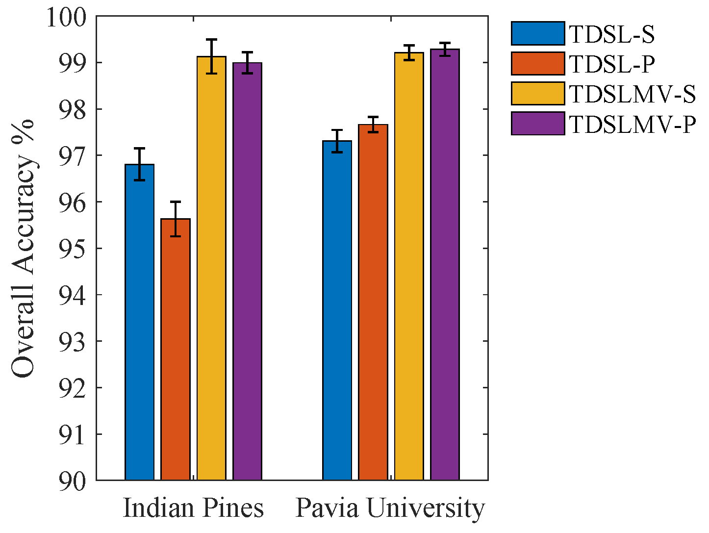
To discuss the performance of the proposed methods when meeting the cross-scene and cross-sensor classification tasks, we display the OA of the proposed methods on the two data sets in Figure 11. It can be easily observed that on the Indian Pines data, TDSL-S and TDSLMV-S provide higher OA than TDSL-P and TDSLMV-P, respectively. Whereas, on the Pavia University data, the accuracies of TDSL-P and TDSLMV-P are higher than those of TDSL-S and TDSLMV-S, respectively. This means that the proposed methods provide higher accuracies for the cross-scene task than for the cross-scene and cross-sensor tasks. Furthermore, applying the majority vote not only can refine the classification results, but also close the gaps of accuracies caused by cross-sensor.

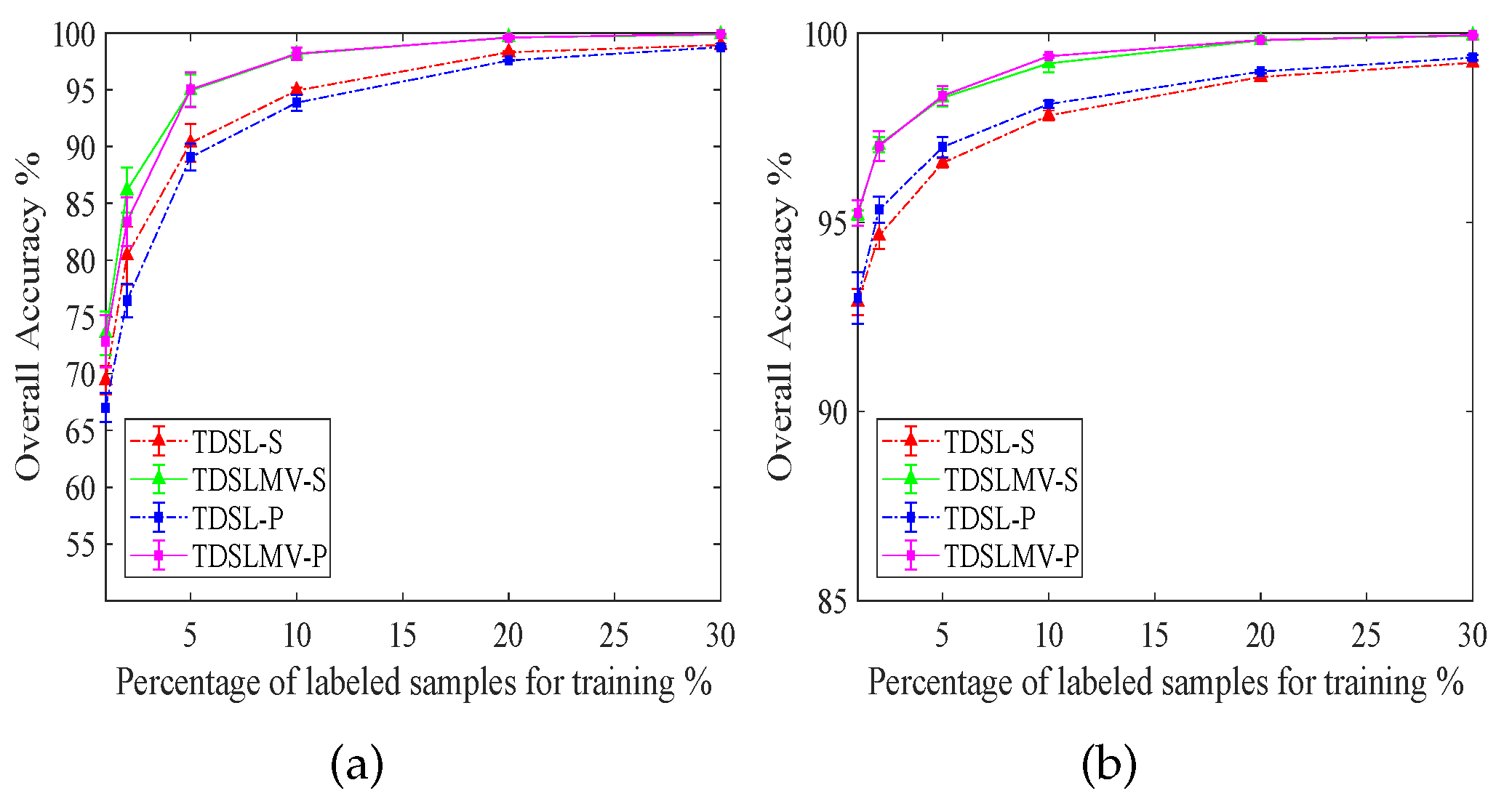
To evaluate the impact of different amounts of labeled training samples from data set #2, we perform all the proposed methods three times with $1\%$, $2\%$, $5\%$, $10\%$, $20\%$, and $30\%$ training samples of the labeled data. We illustrate the results in Figure 12. In Figure 12a, the accuracies with $1\%$ and $2\%$ labeled training samples are not very high on Indian Pines data. Because some classes contain very few samples, for $1\%$, the numbers of labeled training samples in some classes are less than five. However, when the number of labeled training samples gets over $5\%$, the accuracies of TDSLMV are more than $95\%$. In Figure 12b, the accuracies of TDSLMV with $1\%$ labeled training samples can obtain $95\%$ on Pavia University. This demonstrates that our proposed methods can work well with a small labeled training set.

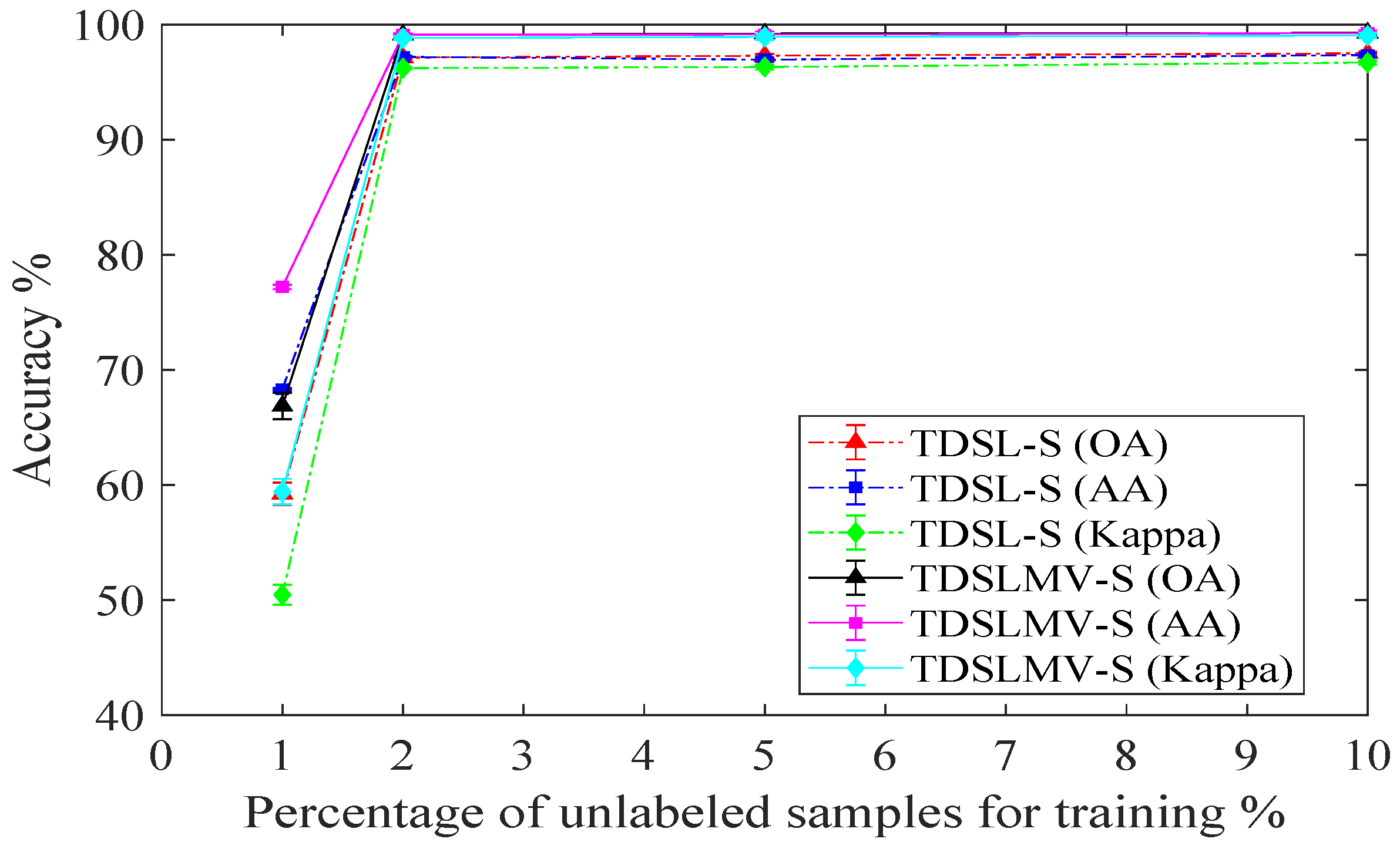
To evaluate the impact of different amounts of unlabeled training samples from data set #1, we perform the proposed TDSL and TDSLMV three times with $1\%$, $2\%$, $5\%$, and $10\%$ training samples from the unlabeled data set Salinas, and we perform classification on Pavia University to evaluate the performance of the feature extractors in cross-scene and cross-sensor classification task. Figure 13 displays the results. The accuracies with $1\%$ unlabeled training samples from Salinas are not very high, the OA of TDSL-S is about $60\%$, and the OA of TDSLMV-S is lower than $70\%$. This demonstrates that when the amount of unlabeled samples is too small, the trained feature extractors can not extract effective generalization features but the accuracies with $2\%$ unlabeled training samples from Salinas are very high, and the number of unlabeled training samples is about 1000. This demonstrates that at least a thousand unlabeled samples are needed to train the feature extractors.

We report the time of the aforementioned methods in Table 7. It is easily observed that SVM is the fastest among these methods, CSVM and GTR are the second-fastest methods. The speeds of SDL, SADL, and ASTDL-CNN are slower than SVM, CSVM, and GTR, because the dictionary learning and sparse representation methods need more time. In SOMP, testing samples are sparsely represented by training samples directly, therefore, it does not need training time. In general, neural network methods need much time to train the model, therefore, the training time of HybridSN is the longest. SpectralFormer needs less training time than HybridSN and ASTDL-CNN, because the input of SpectralFormer is the spectrum, and the number of parameters in the model is small. The training time of ASTDL-CNN is shorter than HybridSN, because ASTDL simplifies the 2-D CNN. The proposed methods take the most time except HybridSN and ASTDL-CNN. The training time of TDSL and TDSLMV includes the time of training dictionaries, the time of sparse representation for labeled training samples, and the time of training SVM. The testing time of TDSL includes the time of sparse representation for testing samples and the time of classification with SVM. The testing time of TDSLMV includes the extra time of the majority vote than TDSL. Although the proposed methods are not the fastest, they provide high accuracies and can complete the cross-scene and cross-sensor classification tasks. Therefore, for applications that are not time critical the proposed methods have distinct advantages.

According to the above experimental results and analysis, the proposed TDLSMV achieves the highest classification accuracies, including the OA, AA, and Kappa, on both Indian Pines and Pavia University in all compared methods. Additionally, the standard deviations of TDSL and TDSLMV are smaller than the other compared methods. It demonstrates the robustness of the proposed methods. Furthermore, TDSL and TDSLMV can achieve high accuracies with a small labeled training set. The disadvantage of the proposed TDSL and TDSLMV is that their speeds are not the fastest.

4.6. Application on a Complex Dataset

We evaluate the classification performance of the trained feature extractor model applied to the Houston2013 dataset directly. The trained feature extractor models come from the aforementioned comparison experiments, in which the feature extractor models are trained on Salinas and Pavia Center data, and the parameters ${\mu }_1$ and ${\mu }_2$ are set as those in experiments on Indian Pines and Pavia University data, i.e., ${\mu }_1$ and ${\mu }_2$ are set as in Table 4. We just use the Houston2013 data to retrain the SVM model, because it is necessary for a classification task. Further, the window size of the majority vote is set as $W=7$, which is the same as in experiments on Pavia University data.

Table 7. Speeds (Seconds) of different methods on the two data sets (the Indian Pines and the Pavia University).

Data Set		SVM [17]	CSVM [50]	SDL [12]	SOMP [14]	SADL [13]	GTR [58]	HybridSN [22]	ASTDL-CNN [61]	SpectralFormer [32]	TDSL-S	TDSL-P	TDSLMV-S	TDSLMV-P
Indian Pines	training time	0.38	2.29	869.55	—	126.19	4.35	3786.11	1543.04	216.96	565.21	329.99	565.21	329.99
	testing time	3.16	3.34	27.95	116.90	7.16	3.43	248.39	126.18	0.91	717.88	748.80	718.37	749.34
Pavia University	training time	0.74	8.49	833.13	—	482.50	4.98	3328.64	1972.61	1425.93	777.43	964.78	777.43	964.78
	testing time	7.54	22.08	97.42	447.06	134.82	16.62	265.37	181.16	2.479	885.61	1466.14	888.17	1468.62

Table 7. Speeds (Seconds) of different methods on the two data sets (the Indian Pines and the Pavia University).

Data Set		SVM [17]	CSVM [50]	SDL [12]	SOMP [14]	SADL [13]	GTR [58]	HybridSN [22]	ASTDL-CNN [61]	SpectralFormer [32]	TDSL-S	TDSL-P	TDSLMV-S	TDSLMV-P
Indian Pines	training time	0.38	2.29	869.55	—	126.19	4.35	3786.11	1543.04	216.96	565.21	329.99	565.21	329.99
	testing time	3.16	3.34	27.95	116.90	7.16	3.43	248.39	126.18	0.91	717.88	748.80	718.37	749.34
Pavia University	training time	0.74	8.49	833.13	—	482.50	4.98	3328.64	1972.61	1425.93	777.43	964.78	777.43	964.78
	testing time	7.54	22.08	97.42	447.06	134.82	16.62	265.37	181.16	2.479	885.61	1466.14	888.17	1468.62

Table 8. Classification accuracies of the proposed methods and SpectralFormer method on Houston2013 dataset.

Class	SpectralFormer [32]	TDSL-S		TDSL-P		TDSLMV-S		TDSLMV-P
		${\mu }_{\mathbf{1}}=\mathbf{0}.\mathbf{008}$ ${\mu }_{\mathbf{2}}=\mathbf{0}.\mathbf{01}$	${\mu }_{\mathbf{1}}=\mathbf{0}.\mathbf{026}$ ${\mu }_{\mathbf{2}}=\mathbf{0}.\mathbf{008}$	${\mu }_{\mathbf{1}}=\mathbf{0}.\mathbf{035}$ ${\mu }_{\mathbf{2}}=\mathbf{0}.\mathbf{0087}$	${\mu }_{\mathbf{1}}=\mathbf{0}.\mathbf{032}$ ${\mu }_{\mathbf{2}}=\mathbf{0}.\mathbf{0089}$	${\mu }_{\mathbf{1}}=\mathbf{0}.\mathbf{008}$ ${\mu }_{\mathbf{2}}=\mathbf{0}.\mathbf{01}$	${\mu }_{\mathbf{1}}=\mathbf{0}.\mathbf{026}$ ${\mu }_{\mathbf{2}}=\mathbf{0}.\mathbf{008}$	${\mu }_{\mathbf{1}}=\mathbf{0}.\mathbf{035}$ ${\mu }_{\mathbf{2}}=\mathbf{0}.\mathbf{0087}$	${\mu }_{\mathbf{1}}=\mathbf{0}.\mathbf{032}$ ${\mu }_{\mathbf{2}}=\mathbf{0}.\mathbf{0089}$
1	84.14	92.89	98.32	99.36	98.40	100.00	100.00	100.00	98.16
2	97.46	95.06	100.00	98.41	99.92	100.00	100.00	99.68	100.00
3	99.60	98.42	99.86	99.14	100.00	100.00	100.00	100.00	100.00
4	97.92	92.04	98.23	95.74	99.44	97.83	100.00	99.68	100.00
5	96.50	98.31	100.00	100.00	100.00	100.00	100.00	100.00	100.00
6	95.10	100.00	99.08	99.08	99.69	100.00	100.00	100.00	100.00
7	87.50	89.43	99.13	92.67	98.97	99.45	100.00	99.37	100.00
8	51.57	80.31	98.55	88.50	99.36	92.28	99.28	94.29	100.00
9	69.50	83.71	99.76	88.18	98.16	94.25	100.00	94.81	99.28
10	81.27	87.53	99.84	87.61	99.84	100.00	100.00	94.46	100.00
11	86.43	90.28	99.76	84.21	99.60	98.22	100.00	92.96	100.00
12	66.09	93.27	99.68	93.03	99.51	99.03	99.68	98.46	99.68
13	75.44	88.06	98.93	90.83	100.00	98.72	100.00	100.00	100.00
14	99.60	97.43	98.36	100.00	100.00	100.00	100.00	100.00	100.00
15	98.73	93.48	100.00	99.85	100.00	100.00	100.00	100.00	100.00
OA	83.64	91.14	99.33	93.67	99.43	98.39	99.91	97.83	99.76
AA	85.79	92.01	99.30	94.44	99.53	98.65	99.93	98.25	99.81
Kappa	82.28	90.43	99.28	93.16	99.38	98.26	99.91	97.66	99.74

displays the classification results of the SpectralFormer method and the trained model of the proposed methods. The models of TDSL-S and TDSLMV-S with ${\mu }_1=0.008$, ${\mu }_2=0.01$, TDSL-P and TDSLMV-P with ${\mu }_1=0.035,{\mu }_2=0.0087$, are the models trained in the aforementioned comparison experiments on Indian Pines. The models of TDSL-S and TDSLMV-S with ${\mu }_1=0.026,{\mu }_2=0.008$, TDSL-P and TDSLMV-P with ${\mu }_1=0.032$, ${\mu }_2=0.0089$, are the models trained in the aforementioned comparison experiments on Pavia University data. It is obvious that the trained model is efficient when applied to a new dataset. The results of the trained models are superior to the results of SpectralFormer. In particular, the OAs of models trained in the experiments on Pavia University are more than $99\%$. The results of models trained in the experiments on Pavia University are better than the results of models trained in the experiments on Indian Pines. It is because the Houston2013 and Pavia University are both gathered over the city, while Indian Pines just contains agriculture, forest, and natural perennial vegetation. The classification results of the TDSLMV model trained in the experiments on Indian Pines achieve $98.39\%$ and $97.83\%$, which are enough for general applications.

Figure 14 shows the three-band false-color composite image, ground truth map, classification maps, and the corresponding error maps for the Houston2013 dataset. Figure 14a shows that the dataset is complex and the labeled categories are scattered. The classification map of SpectralFormer has many misclassified pixels, and the classification maps of the trained models just have a few misclassified pixels. This demonstrates that the trained feature extractor models are efficient when applied to a complex dataset.

5. Conclusions

This paper has proposed an STDL algorithm and a TDSL classification method based on the STDL for HSI. The proposed STDL algorithm initializes dictionaries with TKD and updates dictionaries based on K-HOSVD. The proposed TDSL method utilizes a small amount of unlabeled data to train tensorial feature extractors with the STDL algorithm and then utilizes these feature extractors to extract discriminative joint spectral-spatial tensor features on the other data set. To provide the classification results, SVM is applied to the tensor features. Compared to traditional self-taught learning methods, the proposed method just utilizes a small amount of unlabeled and labeled data. Furthermore, the proposed TDSLMV refines the classification with the majority vote on the classification map obtained by TDSL. The proposed methods have been evaluated on four widely used benchmark data sets and TDSLMV provides the highest accuracies, the average OA of TDSLMV achieves as high as $99.13\%$ and $99.28\%$ on Indian Pines and Pavia University, respectively. The experimental results demonstrate that the proposed methods can complete the cross-scene and cross-sensor classification tasks with high accuracy. TDSLMV can effectively reduce the misclassified pixels in the homogenous regions and at the edges of different homogenous regions, compared with other classification methods, and the average OA is improved by at least $2.5\%$. Moreover, accuracies of the trained feature extractor models applied directly to the classification task on Houston2013 reach $99\%$. When the proposed method is applied to a classification task with limited data, the feature extractor models can be trained on a publicly available dataset and directly applied to the task data. The proposed method can alleviate the problem of limited data. Because of the speeds of the proposed methods, the future work of this research focuses on accelerating dictionary learning and sparse representation.

References

- Primpke, S.; Godejohann, M.; Gerdts, G. Rapid identification and quantification of microplastics in the environment by quantum cascade laser-based hyperspectral infrared chemical imaging. Environ. Sci. Technol. 2020, 54, 15893–15903. [Google Scholar] [CrossRef] [PubMed]
- Safari, K.; Prasad, S.; Labate, D. A multiscale deep learning approach for high-resolution hyperspectral image classification. IEEE Geosci. Remote Sens. Lett. 2021, 18, 167–171. [Google Scholar] [CrossRef]
- Wang, M.; Wang, Q.; Chanussot, J.; Li, D. Hyperspectral image mixed noise removal based on multidirectional low-rank modeling and spatial-spectral total variation. IEEE Trans. Geosci. Remote Sens. 2021, 59, 488–507. [Google Scholar] [CrossRef]
- Gopinath, G.; Sasidharan, N.; Surendran, U. Landuse classification of hyperspectral data by spectral angle mapper and support vector machine in humid tropical region of India. Earth Sci. Inform. 2020, 13, 633–640. [Google Scholar] [CrossRef]
- Wang, M.; Wang, Q.; Chanussot, J. Tensor low-rank constraint and l0 total variation for hyperspectral Image Mixed Noise Removal. IEEE J. Sel. Top. Signal Process. 2021, 15, 718–733. [Google Scholar] [CrossRef]
- Ma, N.; Peng, Y.; Wang, S. A fast recursive collaboration representation anomaly detector for hyperspectral image. IEEE Geosci. Remote Sens. Lett. 2019, 16, 588–592. [Google Scholar] [CrossRef]
- Li, Y.; Zhang, H.; Shen, Q. Spectral-spatial classification of hyperspectral imagery with 3D convolutional neural network. Remote Sens. 2017, 9, 67. [Google Scholar] [CrossRef]
- Kemker, R.; Kanan, C. Self-taught feature learning for hyperspectral image classification. IEEE Trans. Geosci. Remote Sens. 2017, 55, 2693–2705. [Google Scholar] [CrossRef]
- Plaza, A.; Martinez, P.; Plaza, J.; Perez, R. Dimensionality reduction and classification of hyperspectral image data using sequences of extended morphological transformations. IEEE Trans. Geosci. Remote Sens. 2005, 43, 466–479. [Google Scholar] [CrossRef]
- Falco, N.; Benediktsson, J.A.; Bruzzone, L. A study on the effectiveness of different independent component analysis algorithms for hyperspectral image classification. IEEE J. Sel. Top. Appl. Earth Observ. Remote Sens. 2014, 7, 2183–2199. [Google Scholar] [CrossRef]
- Shen, L.; Zhu, Z.; Jia, S.; Zhu, J.; Sun, Y. Discriminative gabor feature selection for hyperspectral image classification. IEEE Geosci. Remote Sens. Lett. 2013, 10, 29–33. [Google Scholar] [CrossRef]
- Charles, A.S.; Olshausen, B.A.; Rozell, C.J. Learning sparse codes for hyperspectral imagery. IEEE J. Sel. Top. Signal Process. 2011, 5, 963–978. [Google Scholar] [CrossRef]
- Soltani-Farani, A.; Rabiee, H.R.; Hosseini, S.A. Spatial-aware dictionary learning for hyperspectral image classification. IEEE Trans. Geosci. Remote Sens. 2015, 53, 527–541. [Google Scholar] [CrossRef]
- Chen, Y.; Nasrabadi, N.M.; Tran, T.D. Hyperspectral image classification using dictionary-based sparse representation. IEEE Trans. Geosci. Remote Sens. 2011, 49, 3973–3985. [Google Scholar] [CrossRef]
- Peng, J.; Sun, W.; Du, Q. Self-paced joint sparse representation for the classification of hyperspectral images. IEEE Trans. Geosci. Remote Sens. 2019, 57, 1183–1194. [Google Scholar] [CrossRef]
- Tao, C.; Pan, H.; Li, Y.; Zou, Z. Unsupervised spectral-spatial feature learning with stacked sparse autoencoder for hyperspectral imagery classification. IEEE Geosci. Remote Sens. Lett. 2015, 12, 2438–2442. [Google Scholar]
- Melgani, F.; Bruzzone, L. Classification of hyperspectral remote sensing images with support vector machines. IEEE Trans. Geosci. Remote Sens. 2004, 42, 1778–1790. [Google Scholar] [CrossRef]
- Chen, Y.; Jiang, H.; Li, C.; Jia, X.; Ghamisi, P. Deep feature extraction and classification of hyperspectral images based on convolutional neural networks. IEEE Trans. Geosci. Remote Sens. 2016, 54, 6232–6251. [Google Scholar] [CrossRef]
- Tang, H.; Li, Y.; Huang, Z.; Zhang, L.; Xie, W. Fusion of multidimensional CNN and handcrafted features for small-sample hyperspectral image classification. Remote Sens. 2022, 14, 3796. [Google Scholar] [CrossRef]
- Ge, Z.; Cao, G.; Zhang, Y.; Shi, H.; Liu, Y.; Shafique, A.; Fu, P. Subpixel multilevel scale feature learning and adaptive attention constraint fusion for hyperspectral image classification. Remote Sens. 2022, 14, 3670. [Google Scholar] [CrossRef]
- Wang, A.; Xing, S.; Zhao, Y.; Wu, H.; Iwahori, Y. A hyperspectral image classification method based on adaptive spectral spatial kernel combined with improved vision transformer. Remote Sens. 2022, 14, 3705. [Google Scholar] [CrossRef]
- Roy, S.K.; Krishna, G.; Dubey, S.R.; Chaudhuri, B.B. HybridSN: Exploring 3-D–2-D CNN feature hierarchy for hyperspectral image classification. IEEE Geosci. Remote Sens. Lett. 2020, 17, 277–281. [Google Scholar] [CrossRef]
- Hong, D.; Gao, L.; Yokoya, N.; Yao, J.; Chanussot, J.; Du, Q.; Zhang, B. More diverse means better: Multimodal deep learning meets remote-sensing imagery classification. IEEE Trans. Geosci. Remote Sens. 2021, 59, 4340–4354. [Google Scholar] [CrossRef]
- Wu, X.; Hong, D.; Chanussot, J. Convolutional neural networks for multimodal remote sensing data classification. IEEE Trans. Geosci. Remote Sens. 2022, 60, 1–10. [Google Scholar] [CrossRef]
- Yao, D.; Zhi-li, Z.; Xiao-feng, Z.; Wei, C.; Fang, H.; Yao-ming, C.; Cai, W.W. Deep hybrid: Multi-graph neural network collaboration for hyperspectral image classification. Def. Technol. 2022, 1–13. [Google Scholar] [CrossRef]
- Mou, L.; Ghamisi, P.; Zhu, X.X. Deep recurrent neural networks for hyperspectral image classification. IEEE Trans. Geosci. Remote Sens. 2018, 56, 1214–1215. [Google Scholar] [CrossRef]
- Shi, C.; Pun, C. Multiscale superpixel-based hyperspectral image classification using recurrent neural networks with stacked autoencoders. IEEE Trans. Multimed. 2020, 22, 487–501. [Google Scholar] [CrossRef]
- Hong, D.; Gao, L.; Yao, J.; Zhang, B.; Plaza, A.; Chanussot, J. Graph convolutional networks for hyperspectral image classification. IEEE Trans. Geosci. Remote Sens. 2021, 59, 5966–5978. [Google Scholar] [CrossRef]
- Ding, Y.; Zhao, X.; Zhang, Z.; Cai, W.; Yang, N. Multiscale graph sample and aggregate network with context-aware learning for hyperspectral image classification. IEEE J. Sel. Top. Appl. Earth Obs. Remote Sens. 2021, 14, 4561–4572. [Google Scholar] [CrossRef]
- Ding, Y.; Zhang, Z.; Zhao, X.; Hong, D.; Li, W.; Cai, W.; Zhan, Y. AF2GNN: Graph convolution with adaptive filters and aggregator fusion for hyperspectral image classification. Inf. Sci. 2022, 602, 201–219. [Google Scholar] [CrossRef]
- Ding, Y.; Zhang, Z.; Zhao, X.; Hong, D.; Cai, W.; Yu, C.; Yang, N.; Cai, W. Multi-feature fusion: Graph neural network and CNN combining for hyperspectral image classification. Neurocomputing 2022, 501, 246–257. [Google Scholar] [CrossRef]
- Hong, D.; Han, Z.; Yao, J.; Gao, L.; Zhang, B.; Plaza, A.; Chanussot, J. Spectralformer: Rethinking hyperspectral image classification with transformers. IEEE Trans. Geosci. Remote Sens. 2022, 60, 1–15. [Google Scholar] [CrossRef]
- Liu, X.; Hong, D.; Chanussot, J.; Zhao, B.; Ghamisi, P. Modality translation in remote sensing time series. IEEE Trans. Geosci. Remote Sens. 2022, 60, 1–14. [Google Scholar] [CrossRef]
- Liu, B.; Yu, X.; Zhang, P.; Tan, X.; Yu, A.; Xue, Z. A semi-supervised convolutional neural network for hyperspectral image classification. Remote Sens. Lett. 2017, 8, 839–848. [Google Scholar] [CrossRef]
- Hong, D.; Yokoya, N.; Xia, G.S.; Chanussot, J.; Zhu, X.X. X-ModalNet: A semi-supervised deep cross-modal network for classification of remote sensing data. ISPRS J. Photogramm. Remote Sens. 2020, 167, 12–23. [Google Scholar] [CrossRef] [PubMed]
- Ding, Y.; Zhao, X.; Zhang, Z.; Cai, W.; Yang, N.; Zhan, Y. Semi-supervised locality preserving dense graph neural network with ARMA filters and context-aware learning for hyperspectral image classification. IEEE Trans. Geosci. Remote Sens. 2022, 60, 1–12. [Google Scholar] [CrossRef]
- Aydemir, M.S.; Bilgin, G. Semi-supervised sparse representation classifier ((SRC)-R-3) with deep features on small sample sized hyperspectral images. Neurocomputing 2020, 399, 213–226. [Google Scholar] [CrossRef]
- Rajan, S.; Ghosh, J.; Crawford, M.M. An active learning approach to hyperspectral data classification. IEEE Trans. Geosci. Remote Sens. 2008, 46, 1231–1242. [Google Scholar] [CrossRef]
- Du, B.; Wang, Z.; Zhang, L.; Zhang, L.; Liu, W.; Shen, J.; Tao, D. Exploring representativeness and informativeness for active learning. IEEE T. Cybern. 2017, 47, 14–26. [Google Scholar] [CrossRef]
- Raina, R.; Battle, A.; Lee, H.; Packer, B.; Ng, A.Y. Self-taught learning: Transfer learning from unlabeled data. In Proceedings of the 24th International Conference on Machine Learning, Corvalis, OR, USA, 20–24 June 2007; pp. 759–766. [Google Scholar]
- He, X.; Chen, Y.; Ghamisi, P. Heterogeneous transfer learning for hyperspectral image classification based on convolutional neural network. IEEE Trans. Geosci. Remote Sens. 2020, 58, 3246–3263. [Google Scholar] [CrossRef]
- Deng, C.; Xue, Y.; Liu, X.; Li, C.; Tao, D. Active transfer learning network: A unified deep joint spectral-spatial feature learning model for hyperspectral image classification. IEEE Trans. Geosci. Remote Sens. 2019, 57, 1741–1754. [Google Scholar] [CrossRef] [Green Version]
- Windrim, L.; Melkumyan, A.; Murphy, R.J.; Chlingaryan, A.; Ramakrishnan, R. Pretraining for hyperspectral convolutional neural network classification. IEEE Trans. Geosci. Remote Sens. 2018, 56, 2798–2810. [Google Scholar] [CrossRef]
- Yang, J.; Zhao, Y.Q.; Chan, J.C.W. Learning and transferring deep joint spectral-spatial features for hyperspectral classification. IEEE Trans. Geosci. Remote Sens. 2017, 55, 4729–4742. [Google Scholar] [CrossRef]
- Deng, B.; Jia, S.; Shi, D. Deep metric learning-based feature embedding for hyperspectral image classification. IEEE Trans. Geosci. Remote Sens. 2020, 58, 1422–1435. [Google Scholar] [CrossRef]
- Jiang, Y.; Li, Y.; Zhang, H. Hyperspectral image classification based on 3-D separable ResNet and transfer learning. IEEE Geosci. Remote Sens. Lett. 2019, 16, 1949–1953. [Google Scholar] [CrossRef]
- Zhong, Z.; Li, J.; Luo, Z.; Chapman, M. Spectral-spatial residual network for hyperspectral image classification: A 3-D deep learning framework. IEEE Trans. Geosci. Remote Sens. 2018, 56, 847–858. [Google Scholar] [CrossRef]
- Kemker, R.; Luu, R.; Kanan, C. Low-shot learning for the semantic segmentation of remote sensing Imagery. IEEE Trans. Geosci. Remote Sens. 2018, 56, 6214–6223. [Google Scholar] [CrossRef]
- Yang, L.; Yang, Y.; Yang, J.; Zhao, N.; Wu, L.; Wang, L.; Wang, T. FusionNet: A convolution-transformer fusion network for hyperspectral image classification. Remote Sens. 2022, 14, 4066. [Google Scholar] [CrossRef]
- Camps-Valls, G.; Gomez-Chova, L.; Munoz-Mari, J.; Vila-Frances, J.; Calpe-Maravilla, J. Composite kernels for hyperspectral image classification. IEEE Geosci. Remote Sens. Lett. 2006, 3, 93–97. [Google Scholar] [CrossRef]
- Tu, X.; Shen, X.; Fu, P.; Wang, T.; Sun, Q.; Ji, Z. Discriminant sub-dictionary learning with adaptive multiscale superpixel representation for hyperspectral image classification. Neurocomputing 2020, 409, 131–145. [Google Scholar] [CrossRef]
- Ghanbari Azar, S.; Meshgini, S.; Yousefi Rezaii, T.; Beheshti, S. Hyperspectral image classification based on sparse modeling of spectral blocks. Neurocomputing 2020, 407, 12–23. [Google Scholar] [CrossRef]
- Li, D.; Wang, Q.; Kong, F. Adaptive kernel sparse representation based on multiple feature learning for hyperspectral image classification. Neurocomputing 2020, 400, 97–112. [Google Scholar] [CrossRef]
- Hong, D.; Yokoya, N.; Chanussot, J.; Zhu, X.X. An augmented linear mixing model to address spectral variability for hyperspectral unmixing. IEEE Trans. Image Process. 2019, 28, 1923–1938. [Google Scholar] [CrossRef] [PubMed]
- Wang, M.; Wang, Q.; Hong, D.; Roy, S.K.; Chanussot, J. Learning tensor low-rank representation for hyperspectral anomaly detection. IEEE Trans. Cybern. 2022, 1–13. [Google Scholar] [CrossRef]
- Hong, D.; Hu, J.; Yao, J.; Chanussot, J.; Zhu, X.X. Multimodal remote sensing benchmark datasets for land cover classification with a shared and specific feature learning model. ISPRS J. Photogramm. Remote Sens. 2021, 178, 68–80. [Google Scholar] [CrossRef]
- Zhao, G.; Tu, B.; Fei, H.; Li, N.; Yang, X. Spatial-spectral classification of hyperspectral image via group tensor decomposition. Neurocomputing 2018, 316, 68–77. [Google Scholar] [CrossRef]
- Liu, J.; Wu, Z.; Xiao, L.; Sun, J.; Yan, H. Generalized tensor regression for hyperspectral image classification. IEEE Trans. Geosci. Remote Sens. 2020, 58, 1244–1258. [Google Scholar] [CrossRef]
- He, Z.; Hu, J.; Wang, Y. Low-rank tensor learning for classification of hyperspectral image with limited labeled samples. Signal Process. 2018, 145, 12–25. [Google Scholar] [CrossRef]
- Liu, F.; Wang, Q. A sparse tensor-based classification method of hyperspectral image. Signal Process. 2020, 168, 1–14. [Google Scholar] [CrossRef]
- Liu, F.; Ma, J.; Wang, Q. Atom-substituted tensor dictionary learning enhanced convolutional neural network for hyperspectral image classification. Neurocomputing 2021, 455, 215–228. [Google Scholar] [CrossRef]
- Cichocki, A.; Mandic, D.; De Lathauwer, L.; Zhou, G.; Zhao, Q.; Caiafa, C.; Phan, H.A. Tensor decompositions for signal processing applications: From two-way to multiway component analysis. IEEE Signal Process. Mag. 2015, 32, 145–163. [Google Scholar] [CrossRef] [Green Version]
- De Lathauwer, L. Decompositions of a higher-order tensor in block terms—part II: Definitions and uniqueness. SIAM J. Matrix Anal. Appl. 2008, 30, 1033–1066. [Google Scholar] [CrossRef]
- Roemer, F.; Del Galdo, G.; Haardt, M. Tensor-based algorithms for learning multidimensional separable dictionaries. In Proceedings of the 2014 IEEE International Conference on Acoustics, Speech and Signal Processing (ICASSP), Florence, Italy, 4–9 May 2014; pp. 3963–3967. [Google Scholar]
- Ding, X.; Chen, W.; Wassell, I.J. Joint sensing matrix and sparsifying dictionary optimization for tensor compressive sensing. IEEE Tran. Signal Process. 2017, 65, 3632–3646. [Google Scholar] [CrossRef]
- De Lathauwer, L.; De Moor, B.; Vandewalle, J. A multilinear singular value decomposition. SIAM J. Matrix Anal. Appl. 2000, 21, 1253–1278. [Google Scholar] [CrossRef]
- Caiafa, C.F.; Cichocki, A. Computing sparse representations of multidimensional signals using Kronecker bases. Neural Comput. 2013, 25, 186–220. [Google Scholar] [CrossRef]
- Bader, B.W.; Kolda, T.G. MATLAB Tensor Toolbox Version 2.5. 2012. Available online: http://www.sandia.gov/~tgkolda/TensorToolbox/ (accessed on 29 November 2018).
- Chang, C.C.; Lin, C.J. LIBSVM: A Library for support vector machines. ACM Trans. Intell. Syst. Technol. 2011, 2, 1–27. [Google Scholar] [CrossRef]
Figure 1.
Flowchart of the tensor-based dictionary self-taught learning classification method with the majority vote (TDSLMV).
Figure 2.
Three-band false-color composite images, ground truth maps, the corresponding sensors, and details of the samples for the four widely used benchmark data sets (the Salinas, the Indian Pines, the Pavia Center, and the Pavia University): (a) false-color composite image of Salinas, (b) ground truth map of Salinas, (c) false-color composite image of Indian Pines, (d) ground truth map of Indian Pines, (e) false-color composite image of Pavia Center, (f) ground truth map of Pavia Center, (g) false-color composite image of Pavia University, (h) ground truth map of Pavia University.
Figure 3.
Impact of the sparsity level in tensor dictionary learning () for the unlabeled data sets #1 (the Salinas and the Pavia Center) and the sparsity level in sparse representation () for the labeled data sets #2 (the Indian Pines and the Pavia University) on the classification accuracies (AA, OA, and Kappa), and the average number of nonzero coefficients in feature tensors (K). From top to bottom, the first row (a–d) represents the results of the TDSL-S on the Indian Pines, the second row (e–h) represents the results of the TDSL-P on the Indian Pines, the third row (i–l) represents the results of the TDSL-S on the Pavia University, and the last row (m–p) represents the results of the TDSL-P on the Pavia University.
Figure 4.
Classification accuracies (the OA, AA, and Kappa) and the average number of nonzero coefficients in feature tensors (K) for TDSL-S on Indian Pines. (a) The effect of when is fixed and . (b) The effect of when is fixed and .
Figure 5.
Classification accuracies (the OA, AA, and Kappa) and the average number of nonzero coefficients in feature tensors (K) for TDSL-P on Indian Pines. (a) The effect of when is fixed and . (b) The effect of when is fixed and .
Figure 6.
Classification accuracies (the OA, AA, and Kappa) and the average number of nonzero coefficients in feature tensors (K) for TDSL-S on Pavia University. (a) The effect of when is fixed and . (b) The effect of when is fixed and .
Figure 7.
Classification accuracies (the OA, AA, and Kappa) and the average number of nonzero coefficients in feature tensors (K) for TDSL-P on Pavia University. (a) The effect of when is fixed and . (b) The effect of when is fixed and .
Figure 8.
Classification accuracies (the OA, AA, and Kappa) for proposed methods with the majority vote in different window sizes (W) on two data sets. (a) The results of TDSLMV-S on Indian Pines. (b) The results of TDSLMV-S on Pavia University. (c) The results of TDSLMV-P on Indian Pines. (d) The results of TDSLMV-P on Pavia University.
Figure 9.
Classification maps and the corresponding error maps obtained by (a) SVM (OA = 81.07%), (b) CSVM (OA = 92.86%), (c) SDL (OA = 76.63%), (d) SOMP (OA = 81.71%), (e) SADL (OA = 91.36%), (f) GTR (OA = 96.75%), (g) HybridSN (OA = 94.29%), (h) ASTDL-CNN (OA = 96.31%), (i) SpectralFormer (OA = 83.61%), (j) TDSL-S (OA = 97.12%), (k) TDSL-P (OA = 96.07%), (l) TDSLMV-S (OA = 99.57%), and (m) TDSLMV-P (OA = 99.25%) for the Indian Pines.
Figure 10.
Classification maps and the corresponding error maps obtained by (a) SVM (OA = 86.24%), (b) CSVM (OA = 90.79%), (c) SDL (OA = 85.80%), (d) SOMP (OA = 87.95%), (e) SADL (OA = 92.07%), (f) GTR (OA = 90.87%), (g) HybridSN (OA = 95.95%), (h) ASTDL-CNN (OA = 96.73%), (i) SpectralFormer (OA = 86.12%), (j) TDSL-S (OA = 97.63%), (k) TDSL-P (OA = 97.95%),(l) TDSLMV-S (OA = 99.45%), and (m) TDSLMV-P (OA = 99.49%) for the Pavia University.
Figure 11.
The overall accuracies of proposed methods TDSL-S, TDSL-P, TDSLMV-S, and TDSLMV-P on the two data sets ( the Indian pines and the Pavia University).
Figure 12.
The overall accuracies of TDSL-S, TDSLMV-S, TDSL-P, and TDSLMV-P with different percentages of labeled samples for training. (a) The results for Indian Pines. (b) The results for Pavia University.
Figure 13.
The classification accuracies (OA, AA, Kappa) of TDSL-S and TDSLMV-S on Pavia University with different percentages of unlabeled training samples from Salinas.
Figure 14.
Three-band false-color composite image, ground truth map, classification maps, and the corresponding error maps obtained by SpectralFormer method and the proposed methods on the Houston2013: (a) false-color composite image and ground truth map, (b) SpectralFormer, (c) TDSL-S with and , (d) TDSL-S with and , (e) TDSL-P with and , (f) TDSL-P with and , (g) TDSLMV-S with and , (h) TDSLMV-S with and , (i) TDSLMV-P with and , (j) TDSLMV-P with and .