
Spatial-Statistical Analysis of Landscape-Level Wildfire Rate of Spread


1
Department of Geography, San Diego State University, San Diego, CA 92182, USA
2
USDA Forest Service, Pacific Southwest Research Station, Riverside, CA 96002, USA
*
Author to whom correspondence should be addressed.
Remote Sens. 2022, 14(16), 3980; https://doi.org/10.3390/rs14163980
Submission received: 27 June 2022
/
Revised: 3 August 2022
/
Accepted: 9 August 2022
/
Published: 16 August 2022
(This article belongs to the Special Issue Landscape Ecology in Remote Sensing)
Abstract
:The objectives of this study were to evaluate spatial sampling and statistical aspects of landscape-level wildfire rate of spread (ROS) estimates derived from airborne thermal infrared imagery (ATIR). Wildfire progression maps and ROS estimates were derived from repetitive ATIR image sequences collected during the 2017 Thomas and Detwiler wildfire events in California. Three separate landscape sampling unit (LSU) sizes were used to extract remotely sensed environmental covariates known to influence fire behavior. Statistical relationships between fire spread rates and landscape covariates were analyzed using (1) bivariate regression, (2) multiple stepwise regression, (3) geographically weighted regression (GWR), (4) eigenvector spatial filtering (ESF) regression, (5) regression trees (RT), and (6) and random forest (RF) regression. GWR and ESF regressions reveal that relationships between covariates and ROS estimates are substantially non-stationary and suggest that the global association of fire spread controls are locally differentiated on landscape scales. Directional slope is by far the most strongly associated covariate of ROS for the imaging sequences analyzed and the size of LSUs has little influence on any of the covariate relationships.
1. Introduction
Fire plays an integral role in many ecosystem processes [1] but can significantly impact environments and communities globally [2,3]. The spatial characteristics of wildfire behavior at landscape scales is an important aspect of fire ecology [4,5], and an important component of wildfire behavior is rate of spread (ROS). Many environmental components influence ROS at landscape scales, including (1) fuels, (2) topography, and (3) weather/fire-induced weather [6,7,8,9]. Airborne thermal infrared (ATIR) imagery provides a useful data source for mapping and estimating fire perimeters [10,11,12,13,14]. Repetitive ATIR imagery combined with terrain- and fuel-related data are useful for studying landscape-level controls and spatial relationships of environmental controls with wildfire behavior [15,16].
Stow et al. [12] illustrated the benefits of directly measuring fire spread by delineating front movements from repeat-pass ATIR imagery. Stow et al. [13] further demonstrated the capabilities of using repeat-ATIR imagery for evaluating landscape-level ROS estimates. They tested several image processing edge-detection filters and manual fire front delineation approaches to document levels of uncertainty and precision with ROS measurements derived from several different wildfires.
Ordinary least square (OLS) regression methods are common in wildfire research [17,18,19,20]. However, OLS models are subjected to assumptions of independent observation and constant variances over space [21], potentially limiting their efficiency for wildfire research [22,23]. Similarly, violation of OLS assumptions from spatial non-stationarity and autocorrelation is common with ecological variables exhibiting dynamic spatial and temporal characteristics [24]. Spatial non-stationarity is observable when a lack of stability over space for a landscape process is exhibited and can violate assumptions of OLS constant variance over space [25,26]. Spatial autocorrelation is defined as the correspondence between variable attributes in geographic space [24,25,26,27]. Spatial autocorrelation is prevalent in wildfire/ecological process modeling and is problematic for classical modeling practices such as OLS that assume independently distributed errors [26,27]. Similarly, spatial autocorrelation can be problematic for linear models by altering parameter estimates when spatially successive sampling structures or observations are present [24,25,26]. Spatial non-stationarity and autocorrelation are equally important for spatial modeling endeavors and should always be considered when investigating dynamic ecological and spatial processes [24,28].
Geographically weighted regression (GWR) regression was developed to account for variable non-stationarity by enabling the estimation of model parameters at separate sample locations, thereby allowing the description of patterns and relationships between variables over space [28]. The incorporation of spatially varying relationships between variables over space using GWR has become increasingly popular and lends itself to the stochastic nature of wildfire behavior [23,29,30]. Eigenvector-based spatial filtering (ESF) regression is a solution to account for spatial autocorrelation by extracting eigenvectors from a distance-connectivity matrix created between spatial units and structured sampling frameworks [31]. These eigenvectors are used to describe the spatial structure of data for a study region and are added as additional predictors of the response variable [31,32]. This allows spatial structures in regression residuals to be considered during the model fitting processes, largely removing any effect of spatial autocorrelation within a model.
The relationship between wildfire spread rates and landscape covariates is inherently complex. Research on the relationship between the environment and wildfire behavior can also be hindered by variable nonlinearity and interactions occurring on different scales [33,34,35]. Subsequently, many fire behavior and ecological studies have employed the use of machine learning (ML) algorithms to better identify complex structures stemming from nonlinear data and variable interactions without having to satisfy the strict assumptions required by traditional parametric modeling approaches [36,37,38]. Regression trees (RTs) [39,40] and random forest (RF) [34,41] are popular tree-based ML algorithms commonly used to study ecological relationships with fire behavior. Tree-based methods involve the partitioning of data into subsets with lower variance than the first, producing a branching structure [42]. However, single-tree models such as RT can exhibit high variance resulting in unstable predictions and poor characterization of variable interactions [42]. Subsequently, small changes in training data can produce significantly different models. To account for the high variance of single tree models, ensemble methods such as bootstrap aggregating (bagging) were created to combine and average multiple single-tree models to build an average predicted tree [43]. However, bagging approaches with RT are still limited by the high correlation of separate trees used to fit the final model [44]. To further accommodate bagging limitations with RT, the RF algorithm was developed by Breiman [44]. RF algorithms add additional randomness to bagging by using random subsets of data that are decorrelated from one another. In contrast to RT, the RF method constructs trees from the most influential variables within each random bootstrap subset by the employment of split-variable randomization. Each tree in a RF provides a single vote of variable importance and is averaged across all trees. RF algorithms usually perform well with little user tuning required, contain built-in validation, and are robust to outliers [42]. However, the RF algorithm can be very slow with large data sets and is less easily interpreted compared to RT [42].
Schag et al. [15] used fire spread vectors connecting sequential fire fronts as landscape sampling units (LSUs) to quantify ROS and sample topographic and fuel covariates. In that study, variable stratification with bivariate and multiple stepwise regression were used to analyze ROS estimates and landscape covariates. They found that directional slope was the most significant explanatory variable of fire spread rates, while image-derived fuel surrogates, composed of spectral vegetation indices (SVIs) and growth form maps, explained little variance in ROS. Schag et al. (2021) [15] determined that measurements of wind speed and direction and relative humidity are too spatially and temporally coarse to be included as covariates for statistical analyses of fire rate of spread at the landscape scales at which fire behavior was evaluated. This study builds on the work of Schag et al. (2021) [15], with the objective of assessing the effects of different spatial sampling unit sizes and the utility of different spatial and ML models in assessing landscape-scale environmental controls on ROS estimates derived from ATIR imagery.
2. Materials and Methods
2.1. Study Areas
The study areas for this research are found within localized burn extents of the 2017–2018 California Thomas and Detwiler wildfires where time sequential ATIR imagery was collected, as shown in Figure 1. The Thomas Fire burned from 4 December 2017 to 12 January 2018, in Santa Barbara and Ventura counties [45]. The Detwiler fire burned over 30,000 ha in Mariposa County from 16 July to 29 August 2017. The study areas are composed of mountainous topography with significant variations in slope angle and aspect. Chaparral, coastal sage scrub, and oak woodland fuel types were prevalent within the burn extents of the wildfires.
2.2. Airborne Thermal Infrared (ATIR) Imagery and Processing
ATIR imagery was collected with the FireMapper 2.0 thermal infrared imaging system. The FireMapper 2.0 system is a compact fire imaging radiometer that uses a microbolometer focal-plan array (BAE Systems, Inc., Falls Church, VA, USA), providing thermal-infrared imagery from 9 to 12.5 μm [46]. Imaging flight lines were oriented perpendicular to the general direction of wildfire spread (and commonly the predominant wind direction) [13] to sequentially image active fire fronts at time intervals between 6 and 45 min, depending on the apparent fire spread direction during image acquisition (Figure 2).
Although we collected FireMapper 2.0 imagery for four days of the Thomas Fire, we prioritized imagery selection for ROS analyses based on imaged areas with a high number of repetitive flight-passes at fire fronts. FireMapper imagery was geometrically corrected using onboard positional (global navigation satellite system) and attitude (inertial motion unit) data and provided in the form of orthomosaics and georeferenced image frames, as described in Schag et al. [15]. The selected ATIR images were acquired on 8–9 December 2017. Four separate image sequences ranging between 7 and 26 repetitive passes were processed and analyzed; these are referred to as Thomas Sequences 1 through 4 (Figure 2). The imagery has a nominal ground sample distance (GSD) of 10 m. The average time between successive imaging passes ranged from 6 to 10 min. A seven-image sequence captured with a nominal GSD of 13 m and repeat pass intervals of 7 to 9 min for the Detwiler Fire on 20 July 2017 was also analyzed. The root mean square error of co-registration of sequential FireMapper 2.0 image pairs is approximately 1–2 pixels [13].
2.3. Geospatial Data
Visible and near infrared orthoimagery and digital elevation model data were sources for mapping surrogates for fuel load and condition and topography, respectively. Pre-fire National Agricultural Inventory Program (NAIP) imagery (extracted from the USGS earth explorer tool (https://earthexplorer.usgs.gov/, accessed 1 August 2020), with a GSD of 0.6 m captured in July and August of 2016, were used to generate SVI images and map vegetation growth form types. Digital elevation models (DEMs) with 10 m (1/3 arc seconds) rasters were retrieved from the United States Geological Survey (USGS) National Elevation Dataset (NED). The NED-DEMs were used to generate a topographic landscape variable, directional slope, which was found by Schag et al. [15] to be highly correlated with ROS.
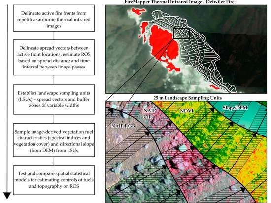
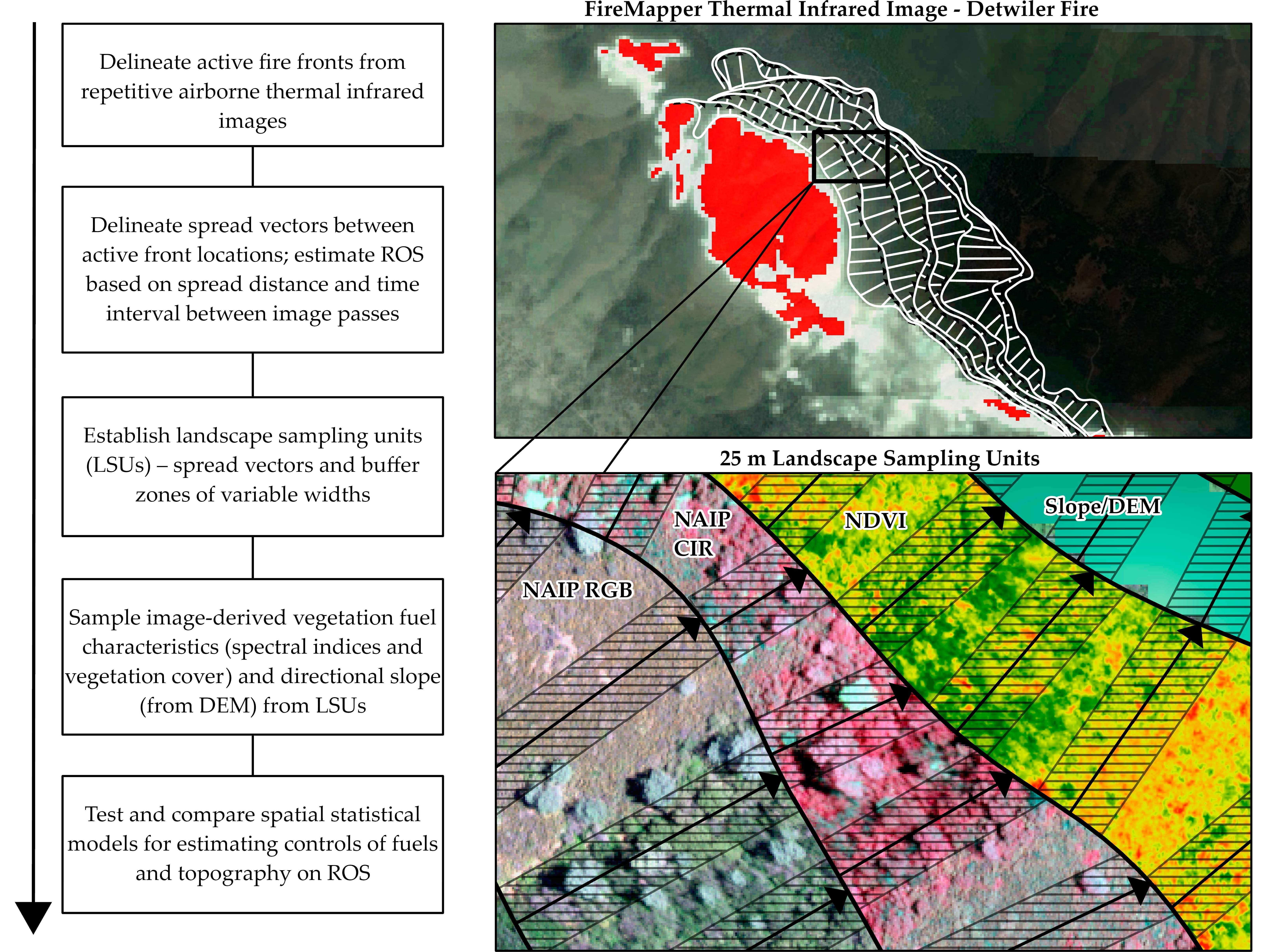
2.4. Fire Front, Spread Vector, and Landscape Sampling Unit (LSU) Delineation
Fire front locations were delineated from co-registered, repeat-pass ATIR image following procedures developed by Stow et al. [12,13] and conducted in Schag et al. [15]. Contrast enhancements were applied to ATIR images, enabling polylines to be manually delineated and digitized.
Fire spread vectors were used as the geographic units to calculate ROS and connect sequential fire fronts [13], as illustrated in Figure 3. Evenly spaced points along a time = n front curve every 30 m were automatically generated by local-normal polyline connections along each individual point until extension to the intersection of the time = n + 1 fire front. Spread vectors were then generated using the Perpendicular Distance tool (ArcMap 10.4.1) and assigned geometry attributes in the form of a line bearing (0–360°), vector start (x,y and front ID), vector end (x,y and front ID), vector centroid (x,y), and distance (m). Associated with each spread vector is an estimate of ROS (m min−1), calculated as the vector magnitude divided by the time interval between sequential images [13].
We refer to the spatial units of analysis for comparing ROS estimates to landscape covariates as LSUs, which were created using the “Buffer” tool in ArcGIS Pro. Three separate LSU sizes including (1) spread vector pixels, (2) 25 m buffers, and (3) 50 m buffers were used for sampling and analyzing landscape covariates. LSUs have spatial geometry attributes consisting of the fire spread bearing, the length of the unit, and the unit’s size (m2). An example of 25 m LSUs separated along fire fronts is depicted in Figure 3b. The derivation of LSU sizes used in this study was determined from findings from Stow et al. [13] and Schag et al. [15] to capture the variance of landscape-scale influences of fire spread rates calculated from the ATIR image sequences.
2.5. Image Derived Fuel Covariates
Five SVIs were generated from NAIP images and assessed as surrogates of fuel loading and condition, and/or to classify growth from vegetation types: Normalized Difference Vegetation Index (NDVI) (Equation (1)), Green-Red Vegetation Index (GRVI) (Equation (2)), and Normalized Difference Red-Blue (NDRB) (Equation (3)) images were created for all fire sequences.
where RED, GREEN, and BLUE are uncalibrated NAIP digital number values for red, green, and blue wavebands, respectively. Input data for growth form mapping included Visible Brightness (VB) (Equation (4), the red/green band ratio (RG) (Equation (5), and NDVI. Classification of four growth form and landscape cover types: (1) shrub, (2) herb, (3) tree, and (4) rock/bare soil, was based on SVI thresholds that were determined interactively.
VB = (RED + GREEN + BLUE)
RG = RED/GREEN
2.6. Topographic Data Derived Covariates
Directional slope (°), the slope inclination relative to the fire spread direction, was calculated from NED-DEM data with a customized routine developed by Schag et al. [15]. Directional slope was calculated as:
where DS is the output directional slope raster, S is a raster gird representing slope degree values, VD is the spread vector bearing (degree) raster, and A is the aspect in degrees.
2.7. Landscape Covariate Sampling
We implemented zonal sampling with scripted GIS tools to extract SVI, growth form, and directional slope data for LSUs [47]. Samples were stratified within a database and linked to statistical software to support ROS statistical analyses.
Like-classified, contiguous growth form pixels were grouped and converted into vector polygons. LSUs were then used to clip their coincident growth-form polygons. Finally, the fractional cover (FC) percentage of each growth form (based on the LSU size) was quantified on a scale of 0–1. For example, an LSU with 30% shrub cover, 30% herbaceous cover, 40% rock/barren cover, and 0% tree would be assigned the following units: 0.3-Shrub, 0.3-Herb, 0.4-rock/barren, and 0.0-tree. Growth form fractions within each LSU were then used to assign a “LSU Fuel Class” type to each unit. Fuel classes were based on generalized modifications of several fuel/vegetation classification schemes from several sources [48,49,50].
2.8. Statistical Analyses
We applied bivariate linear regression and geographically weighted regression (GWR) analyses to assess whether relationships between ROS and covariates varied with different sizes of LSUs and compared four different spatial statistical routines for examining multi-covariate relationships. Bivariate regressions were run with linear, exponential, and power models, and evaluated based on beta and standardized beta coefficients (β), adjusted coefficient of determination (adj. R2), Akaike’s Information Criterion (AIC), and p-value diagnostics.
Six statistical algorithms were employed to comprehensively examine relationships between landscape covariates and ROS estimates: (1) bivariate regression, (2) multiple stepwise regression, (3) geographically weighted regression (GWR), (4) eigenvector spatial filtering regression (ESF), (5) regression trees (RTs), and (6) random forest (RF) regression. All statistical analyses except GWR models were conducted using R Statistical Software [51]. Data visualizations and descriptive/inferential statistics were generated with global R functions. The more complex modeling procedures that were implemented with separate downloadable R packages are documented below. All statistical models were fit using covariate sample means derived from LSUs.
GWR models were built using the GWR4 software suite by Nakaya [52]. The best combination of landscape covariates exhibiting the lowest AIC and Mallows CP, highest adj. R2, and significant F-static (identified during forward-and-backward multiple stepwise regression) were used for constructing GWR models. A Gaussian weighting function having an adaptive spatial kernel and AIC minimization bandwidth were used to calibrate all models [53]. The optimal bandwidth was selected using the “Golden Section Search” algorithm. AIC and mean adj. R2 diagnostics were used to examine models.
Although OLS and GWR models use different regression parameters, they can still be evaluated and compared using standard model diagnostics [54]. Candidate models were compared using adj. R2 and AIC diagnostics. Models with the highest adj. R2 and lowest AIC were deemed to have the best fit and performance. The residual sum of squares and residual standard error (RSE) estimates of candidate models were also employed to evaluate and compare model performances. Lower residual error indicated stronger model performance [25]. ANOVA tests were conducted to test the null hypothesis that there was no improvement in GWR over OLS. An F-statistic was computed and, if F was significant (p-value < 0.05), the null hypothesis was rejected, indicating GWR substantially improved model fit over OLS counterparts [55,56]. Local coefficients from GWR models were analyzed to determine variable spatial non-stationarity. If a covariate’s local estimate interquartile range was greater than twice the standard deviation of global model (OLS) estimates, the variable was considered to exhibit significant spatial non-stationarity [55].
ESF regression was conducted in R using the spmoran package [57]. The procedure for fitting ESF models included (1) generating a doubly centered spatial connectivity matrix (MCM) for each LSU sample population, (2) extraction of positive eigenvectors from the MCM matrix, (3) multicollinearity filtering, and (4) model fitting using all original covariates combined with eigenvectors used as co-variables [57]. UTM centroid coordinates for the vector LSUs and polygon-border coordinates for the 25 and 50 m LSUs were used to create doubly centered spatial connectivity matrices for each distinct spread sequence and sample population using the spmoran meig function. Significant spatial proximities for each connectivity matrix (distance-based C in the MCM matrix) were determined using a “Gaussian C matrix whose (i,j)-th element equals exp(–di,j/r)” [57] (p. 6), where di,j is the Euclidean distance between sites i and j, and r is the longest distance in the minimum spanning tree covering the study sites, or spatial structure of LSUs [57,58,59]. Eigenvectors corresponding to positive eigenvalues (λ or MC in MCM > 0) were extracted from MCM matrixes using the meigen function. The λ > 0 threshold was applied to represent all positive spatial dependencies of each data set by characterizing each level of the matrix being indexed by the Moran coefficient (MC) [57,60]. To account for any multicollinearity, only eigenvectors that exhibited a VIF < 10 entered a model. The filtered eigenvectors were then used as control variables, or co-variables, for fitting OLS models. Model R2, AIC, and the beta coefficient were the diagnostics used to interpret and compare ESF models.
Data sets for each study area and LSU sample population were split into training (70%) and testing (30%) groups. RT models were fit with training data using the rpart R package [61]. RTs were first built by producing maximal trees that contained no specified pruning parameters and stopping points. Maximal trees were fit first to examine the range of parameters applied by the default rpart function to a data set with no descriptive information being left out of the training data. Maximal trees commonly overfit data and include considerable noise. For this reason, pruning of maximal trees was conducted using the cost-complexity (CP) criterion parameter [62]. CP determines the optimum RT as a trade-off between a tree’s data fit, training data set size, and the size of the tree (number of terminal nodes) [62]. Optimal RT models were evaluated by the mean square error (MSE), R2, and cross validation (CV)-RMSE and -R2 on corresponding test data. To ensure RT models were not overfitting test data or producing biased estimates, the leave-one-out (LOO) CV-RMSE and R2 were calculated during model construction. LOO is a K-fold CV procedure that trains N (K = N) number of models, leaving one sample out to test prediction. LOO diagnostics are produced from averaging errors across all N models.
RF models were fit with the same training and test sample groups used to construct RT models. RF models were trained and evaluated using the h2o R package [63]. RF models in the h2o package have many tuning parameters including (1) number of trees, (2) the number of variables to randomly sample at each split, (3) the number of training samples, (4) the minimum number of samples at a terminal node, and (5) the maximum number of terminal nodes. To determine the most appropriate parameters for each RF model, full Cartesian grid searches were employed for all models. Full Cartesian grid searches test every combination of model parameters until the model with the lowest MSE and out-of-bag (OOB) test error is found. Optimal RT models were evaluated by the mean square error (MSE), R2, and LOO CV-RMSE and -R2 on corresponding test data. The variable importance (VI) measure was used to determine the relative significance of each covariate on predicting ROS estimates. VI is measured by recording the decrease in MSE every time a variable is used as a node split in a tree and is calculated automatically for RF models in the h2o R package.
3. Results
3.1. Bivariate Relationships
Linear, exponential, power-law, and GWR regression results for ROS on directional slope, structured by study fire, ATIR sequence, and LSU size, are presented in Table 1. We present only the ROS-directional slope relationships, as most of the relationships with image-derived fuel covariates (SVIs and growth form fractions) were not statistically significant and the weakly significant relationship resulted from large sample sizes (n) with adj. R2 < 0.15 and p > 0.05. Significant (p < 0.05) but weak relationships were found for all three SVIs tested (NDVI, GRVI, and NDBR) for the Detwiler and Thomas 4 sequences, and for herb and barren/rock fractions for the Thomas 4 sequence.
Bivariate models of ROS on directional slope were significant for all LSU sizes and all model types (linear, exponential, power, and GWR). Model diagnostics were similar for all LSU sizes; most were only slightly higher for the vector units relative to buffered LSUs. This suggests that LSU size was not a factor for this particular landscape-scale study covariate, as elaborated upon below. Values of adj. R2 were highest for the GWR model and, in general, for Thomas sequences 1–3. Directional slope explained less variance in ROS for the Detwiler sequence that captured mostly downslope spread, and the Thomas 4 sequence where fuel and particularly Santa Ana wind conditions appear to have had greater impact on ROS relative to Thomas sequences 1–3 [15]. Regression, beta, and standardized beta coefficients for all regression methods, LSU sizes, and spread sequences showed positive linear to weakly non-linear relationships between ROS and directional slope. Greater fit by GWR and significant ANOVA tests reveal that the relationship between ROS and directional slope is non-stationary and varies at landscape scales. This relationship did not change significantly with variation in sample size. In addition, the interquartile range of local GWR coefficient estimates for directional slope were consistently greater than twice the standard deviation of global (OLS) model estimates.
3.2. Spatially Weighted and Filtered Regression
GWR and ESF models were fit to all covariate data to (1) assess spatially varied relationships between covariates and ROS estimates, (2) identify possible violations of OLS assumptions stemming from spatial non-stationarity and autocorrelation, and (3) account for/fix any documented occurrences of non-stationarity and spatial autocorrelation. GWR, ESF, and multiple stepwise regression diagnostics are reported in Table 2. ANOVA tests comparing OLS and GWR residuals were significant for all sequences and model groups (p < 0.05).
Significant ANOVA tests between GWR and OLS models reveal that GWR models produce a superior data fit. Local coefficient estimates for covariates from GWR models portray non-stationary relationships with ROS that vary over the spatial extents of imaged sequences. This is further validated by an increase in GWR fits over stepwise models by an average adj. R2 of 0.110. Comparably, ESF improved model fit over GWR counterparts by an average adj. R2 of 0.100. Global Moran’s I tests on bivariate, multiple stepwise, and geographically weighted model residuals exhibited large variations in levels of spatial residual autocorrelation. For multiple stepwise regression models, spatial autocorrelation was most prevalent for 50 m LSU models, and highest for the Detwiler sequence (z-score: 13.552, p-value: < 0.001, Moran’s I: 0.445) and lowest for vector LSU models (Thomas 4: z-score 3.59, p-value: <0.001, Moran’s I: 0.279). All stepwise regression model residuals had significant spatial autocorrelation regardless of LSU size. However, ESF models substantially reduced, or eliminated, spatial autocorrelation of regression model residuals, as shown in Table 3. Not surprisingly, larger LSU sizes increased residual autocorrelation, especially for smaller study areas such as Detwiler and Thomas sequence 3.
Comparisons of ESF and OLS (multiple stepwise regression) coefficients are documented in Table 4. Directional slope relationships with ROS remain largely unchanged between multiple stepwise and ESF regression counterparts; however, vegetation fractional cover and spectral vegetation indices varied significantly between models.
3.3. Machine Learning Regression
To further examine levels of explanatory power, nonlinearity, and variable interactions of individual and combined covariate groups on ROS, two machine learning regression models consisting of regression trees (RTs) and random forest (RF) were trained and evaluated on all five study sequence data sets; these machine learning model results are reported in Table 5. LOO CV-RMSE and -R2 diagnostics consistently demonstrate lower error and stronger prediction when using RF models. Conversely, RT models for the Detwiler sequence are superior for estimating ROS than the corresponding RF model. The lowest RMSE and greatest R2 fit was yielded by the Thomas 3 models. The largest RMSE and lowest R2 resulted for the Thomas 4 group. Measures of variable importance for all models revealed similar patterns of covariate significance previously reported by stepwise regression counterparts. Consistently, RT and RF models added, dropped, or supplemented one to two covariates compared to stepwise models. Directional slope remained the most significant variable for explaining and predicting ROS, followed by herb and shrub fractions, then NDVI, and lastly GRVI.
4. Discussion and Conclusion
This study builds on the work of Stow et al. [12,13] and Schag et al. [15] by assessing whether the size of landscape sampling units impacts statistical relationships between ROS and landscape covariates, and by exploring whether spatially varying and machine learning statistical algorithms better model relationships. The methods utilized to address the research questions included: (1) generating fire progression maps using ATIR image sequences, (2) creating spread vectors to calculate ROS estimates between sequential fire fronts, (3) generating LSUs of varying sizes to extract and analyze fuel and terrain covariates, and (4) analyzing relationships between ROS estimates and covariates using bivariate, multiple regression, spatially weighted and filtered, and machine learning statistical algorithms. The results elucidate relationships between remotely sensed terrain and fuel sampling schemes and landscape-scale wildfire analyses.
4.1. Significance of Covariates and LSU Size
Growth form fractions tended to be stronger explanatory variables of fire spread than SVIs, but generally explained little of the variance in ROS estimates. LSUs within fire spread sequences that contained high herbaceous cover fractions exhibited a positive relationship with ROS, whereas a negative relationship resulted for LSUs with large fractions of trees or rock. This is likely due to homogeneity of vegetation type at the study areas, where sample unit size had little impact on changing these relationships. In contrast to bivariate models, fuel covariates were found to be significant in RT models during CC pruning procedures, which indicates that SVIs and growth forms are necessary for the optimization of single-tree models [38]. In addition, the importance of fuel covariates in ML models are validated by the LOO CV-RMSE and -R2 statistics, indicating that RT and RF models are not overfitted by the incorporation of fuel covariates [39,42]. Improvement in ML predictability and variable-importance diagnostics suggests a nonlinear relationship between the fuel covariates and ROS estimates. The nonlinearity of SVIs and growth forms with ROS may be an artifact of local spatial relationships. GWR regression results indicate that the spatial association between ROS and remotely sensed fuel covariates are highly variable for each study area [22,29]. More specifically, GWR models consistently list interquartile ranges (IQRs) of local coefficient estimates for the fuel covariates as being twice that of the standard deviation of global model (OLS) estimates [54,55]. This indicates that, although SVI and fractional cover of growth forms’ relationships with ROS were weak, the relationships varied significantly over space.
Descriptive analysis of samples in the top 95th percentile of ROS estimates indicates most of the associated LSUs had shrub or herbaceous cover fractions between 90 and 100%. Models based on the 25 and 50 m LSUs consistently yielded higher adj. R2, lower AIC, and lower p-value diagnostics when modeling the effects of shrub and herbaceous cover fractions. Alternatively, model fits were greater with vector rather than buffered LSUs, for areas having higher amounts of rock/barren and tree cover. The differing relationships between fractional cover of growth forms and LSU size with ROS appear to be directly associated with LSU size and the spatial distribution of the variable being sampled. This indicates that a smaller sample size (polyline, vectors) may be more effective for evaluating fractional cover of fuel covariates when sparsely distributed over landscapes. This is likely attributed to higher sampling variances for the smaller spatial unit. Although buffered LSUs yielded greater model fits than vector units when sampling more prevalent growth form types, differences in model coefficients between separate LSU sizes were negligible and should be studied further.
Most regression results on directional slope are generally similar between study areas and sample size. However, stronger fits between ROS and directional slope were documented with the vector sample unit size. This is likely an artifact of the 25 and 50 m samples capturing disparate slope facets and skewing sample statistics. Like the remotely sensed fuel covariates, GWR models reveal significant amounts of spatial non-stationarity on directional slope [22,55]. However, ESF regression coefficients for directional slope are similar between separate study areas and fire sequences (Table 4), indicating that the generalized characteristics of terrain are not as easily influenced by sample size compared to fuel covariates.
4.2. Significance of Combined Covariate Findings
Most of the explanation of the variance by multivariate and ML models is attributed to directional slope, although fuel covariates increased model predictability. This is generally what is understood about fire spread controls; how variations in spread rates are typically the result of complex landscape interactions between fuel, terrain, and weather [64,65,66,67]. To help further explain these combined interactions, RT and RF models were trained and tested using combined covariate data sets. Both RT and RF algorithms consistently explained more variance in ROS estimates than stepwise, GWR, and ESF models. RT and RF models revealed exceptional power and potential for quantifying data nonlinearities, levels of variable importance, covariate interactions, and predicting fire ROS respective of a study sequence’s data used to train and validate a model. We further tested RF model predictability across separate fire events by training RF models with Thomas Fire data and validated them with Detwiler Fire data. The RF models predicted fire spread rates for Detwiler Fire exceptionally well (Test-RMSE High: 16.37 m min−1/Test-RMSE Low: 7.92 m min−1). Overall, the exploratory and predictive capability demonstrated by RF and RT models suggest that machine learning statistical algorithms are valuable tools for landscape scale wildfire spread analyses and prediction [34].
Previous research employing spatially weighted or filtered regression algorithms for fire behavior analysis at landscape scales is limited. An important result stemming from GWR regression is how relationships between covariates and ROS estimates are substantially non-stationary. However, the spatially varying relationships between covariates and ROS are identifiable using GWR and suggest that the global association of fire spread controls are locally differentiated on landscape scales [22]. Further, Moran’s I scores are commonly higher when LSU sizes are larger, likely because buffered LSUs are spaced closer together, and therefore more susceptible to spatial autocorrelation, thus breaking the assumptions of OLS models [24,60]. The varying degrees of spatial autocorrelation (especially with fuel covariates) are attributed to landscape homogeneity and the study’s sampling structure [34]. The incorporation of eigenvectors into a model using ESF regression techniques largely eliminated spatial autocorrelation of model residuals [31,32,60].
4.3. Summary
We demonstrate that the scale of research and sampling structure employed in this study significantly enhances the presence of spatial autocorrelation, and ultimately, modeling errors. An important outcome of this study is that regression and machine learning techniques used to detect and reduce spatial autocorrelation are invaluable for landscape-scale geospatial wildfire behavior research. The landscape ecological modeling techniques implemented in this study substantiate the importance of directional slope in controlling ROS of wildfires burning in chaparral. We demonstrate again that the acquisition and processing of repetitive ATIR imagery of active wildfires provides valuable information about landscape-scale properties and controls on wildfire behavior.
Author Contributions
Conceptualization, G.M.S. and D.A.S.; methodology, G.M.S., D.A.S., A.N. and P.J.R.; software, G.M.S. and A.N.; validation, G.M.S. and P.J.R.; writing—original draft preparation, G.M.S. and D.A.S. writing—review and editing, A.N.; visualization, G.M.S.; supervision, D.A.S.; project administration, D.A.S. and P.J.R.; funding acquisition, D.A.S. and P.J.R. All authors have read and agreed to the published version of the manuscript.
Funding
This research was funded by the National Science Foundation, Division of Social, Behavioral and Economic Research, Geography and Spatial Sciences program (grant no. G00011220). Any opinions, findings, and conclusions or recommendations expressed in this material are the authors’ and do not reflect the views of the NSF.
Data Availability Statement
The data that support the findings of this study are available upon request.
Conflicts of Interest
The authors declare no conflict of interest.
References
- Bowman, D.M.J.S.; Balch, J.K.; Artaxo, P.; Bond, W.J.; Carlson, J.M.; Cochrane, M.A.; D’Antonio, C.M.; DeFries, R.S.; Doyle, J.C.; Harrison, S.P.; et al. Fire in the Earth System. Science 2009, 324, 481–484. [Google Scholar] [CrossRef] [PubMed]
- Viswanathan, S.; Eria, L.; Diunugala, N.; Johnson, J.; McClean, C. An Analysis of Effects of San Diego Wildfire on Ambient Air Quality. J. Air Waste Manag. Assoc. 2006, 56, 56–67. [Google Scholar] [CrossRef] [PubMed]
- Haque, K.; Azad, A.K.; Hossain, Y.; Ahmed, T.; Uddin, M.; Hossain, M. Wildfire in Australia during 2019–2020, Its Impact on Health, Biodiversity and Environment with Some Proposals for Risk Management: A Review. J. Environ. Prot. 2021, 12, 391–414. [Google Scholar] [CrossRef]
- Agee, J.K. The landscape ecology of western forest fire regimes. Northwest Sci. 1998, 72, 24. [Google Scholar]
- Alcasena, F.J.; Salis, M.; Ager, A.A.; Arca, B.; Molina-Terren, D.; Spano, D.; Urdíroz, F.J.A. Assessing Landscape Scale Wildfire Exposure for Highly Valued Resources in a Mediterranean Area. Environ. Manag. 2015, 55, 1200–1216. [Google Scholar] [CrossRef]
- Countryman, C.M. The concept of fire environment. Fire Manag. Today 2004, 64, 49–52. [Google Scholar]
- Albini, F.A. Estimating Wildfire Behavior and Effects; Intermountain Forest and Range Experiment Station General Technical Report; Department of Agriculture, Forest Service: Ogden, UT, USA, 1976. [Google Scholar]
- McKenzie, D.; Miller, C.; Falk, D.A. The Landscape Ecology of Fire; Springer: Dordrecht, The Netherlands, 2011. [Google Scholar]
- Coen, J.L. Some new basics of fire behavior. Fire Manag. Today 2011, 71, 37. [Google Scholar]
- Valero, M.M.; Rios, O.; Pastor, E.; Planas, E. Automated location of active fire perimeters in aerial infrared imaging using unsupervised edge detectors. Int. J. Wildland Fire 2018, 27, 241. [Google Scholar] [CrossRef]
- Ollero, A.; de Dios, J.R.M.; Merino, L. Unmanned aerial vehicles as tools for forest-fire fighting. For. Ecol. Manag. 2006, 234, S263. [Google Scholar] [CrossRef]
- Stow, D.A.; Riggan, P.J.; Storey, E.A.; Coulter, L.L. Measuring fire spread rates from repeat pass airborne thermal infrared imagery. Remote Sens. Lett. 2014, 5, 803–812. [Google Scholar] [CrossRef]
- Stow, D.; Riggan, P.; Schag, G.; Brewer, W.; Tissell, R.; Coen, J.; Storey, E. Assessing uncertainty and demonstrating potential for estimating fire rate of spread at landscape scales based on time sequential airborne thermal infrared imaging. Int. J. Remote Sens. 2019, 40, 4876–4897. [Google Scholar] [CrossRef]
- Riggan, P.J.; Tissell, R.G.; Hoffman, J.W. Application of the FireMapper thermal-imaging radiometer for wildfire suppression. IEEE Aerosp. Conf. Proc. 2003, 4, 1863–1872. [Google Scholar]
- Schag, G.; Stow, D.; Riggan, P.; Tissell, R.; Coen, J. Examining Landscape-Scale Fuel and Terrain Controls of Wildfire Spread Rates Using Repetitive Airborne Thermal Infrared (ATIR) Imagery. Fire 2021, 4, 6. [Google Scholar] [CrossRef]
- Storey, M.A.; Price, O.F.; Sharples, J.J.; Bradstock, R.A. Drivers of long-distance spotting during wildfires in south-eastern Australia. Int. J. Wildland Fire 2020, 29, 459–472. [Google Scholar] [CrossRef]
- Storey, E.A.; Stow, D.A.; Roberts, D.A.; O’Leary, J.F.; Davis, F.W. Evaluating Drought Impact on Postfire Recovery of Chaparral Across Southern California. Ecosystems 2021, 24, 806–824. [Google Scholar] [CrossRef]
- Holmes, T.P.; Huggett, R.J.; Westerling, A.L. Statistical analysis of large wildfires. In The Economics of Forest Disturbances; Springer: Dordrecht, The Netherlands, 2008; pp. 59–77. [Google Scholar] [CrossRef]
- Miller, J.D.; Safford, H. Trends in Wildfire Severity: 1984 to 2010 in the Sierra Nevada, Modoc Plateau, and Southern Cascades, California, USA. Fire Ecol. 2012, 8, 41–57. [Google Scholar] [CrossRef]
- Mirzaei, M.; Bertazzon, S.; Couloigner, I. OLS and GWR LUR models of wildfire smoke using remote sensing and spatiotem-poral data in Alberta. Spat. Knowl. Inf. Can. 2019, 7, 3. [Google Scholar]
- Wagner, H.H.; Fortin, M.-J. Spatial analysis of landscapes: Concepts and statistics. Ecology 2005, 86, 1975–1987. [Google Scholar] [CrossRef]
- Koutsias, N.; Martínez-Fernández, J.; Allgöwer, B. Do Factors Causing Wildfires Vary in Space? Evidence from Geographically Weighted Regression. GIScience Remote Sens. 2010, 47, 221–240. [Google Scholar] [CrossRef]
- Nunes, A.; Lourenço, L.; Castro-Meira, A. Exploring spatial patterns and drivers of forest fires in Portugal (1980–2014). Sci. Total Environ. 2016, 573, 1190–1202. [Google Scholar] [CrossRef]
- Legendre, P. Spatial autocorrelation: Trouble or new paradigm? Ecology 1993, 74, 1659–1673. [Google Scholar] [CrossRef]
- Zhang, L.; Gove, J.H.; Heath, L.S. Spatial residual analysis of six modeling techniques. Ecol. Model. 2005, 186, 154–177. [Google Scholar] [CrossRef]
- Getis, A. A History of the Concept of Spatial Autocorrelation: A Geographer’s Perspective. Geogr. Anal. 2008, 40, 297–309. [Google Scholar] [CrossRef]
- Dormann, C.M.; McPherson, J.B.; Araújo, M.; Bivand, R.; Bolliger, J.; Carl, G.; Kühn, I. Methods to account for spatial auto-correlation in the analysis of species distributional data: A review. Ecography 2007, 30, 609–628. [Google Scholar] [CrossRef]
- Fotheringham, A.S.; Charlton, E.M.; Brunsdon, C. Geographically Weighted Regression: A Natural Evolution of the Expansion Method for Spatial Data Analysis. Environ. Plan. A Econ. Space 1998, 30, 1905–1927. [Google Scholar] [CrossRef]
- Rodrigues, M.; Jiménez-Ruano, A.; Peña-Angulo, D.; de la Riva, J. A comprehensive spatial-temporal analysis of driving factors of human-caused wildfires in Spain using Geographically Weighted Logistic Regression. J. Environ. Manag. 2018, 225, 177–192. [Google Scholar] [CrossRef]
- Su, Z.; Hu, H.; Tigabu, M.; Wang, G.; Zeng, A.; Guo, F. Geographically Weighted Negative Binomial Regression Model Predicts Wildfire Occurrence in the Great Xing’an Mountains Better Than Negative Binomial Model. Forests 2019, 10, 377. [Google Scholar] [CrossRef]
- Borcard, D.; Legendre, P. All-scale spatial analysis of ecological data by means of principal coordinates of neighbor matrices. Ecol. Model. 2002, 153, 51–68. [Google Scholar] [CrossRef]
- Diniz-Filho, J.A.F.; Bini, L.M. Modelling geographical patterns in species richness using eigenvector-based spatial filters. Glob. Ecol. Biogeogr. 2005, 14, 177–185. [Google Scholar] [CrossRef]
- Fang, H.; Srivas, T.; de Callafon, R.A.; Haile, M.A. Ensemble-based simultaneous input and state estimation for nonlinear dynamic systems with application to wildfire data assimilation. Control Eng. Pract. 2017, 63, 104–115. [Google Scholar] [CrossRef]
- Oliveira, S.; Oehler, F.; San-Miguel-Ayanz, J.; Camia, A.; Pereira, J.M. Modeling spatial patterns of fire occurrence in Mediterranean Europe using Multiple Regression and Random Forest. For. Ecol. Manag. 2012, 275, 117–129. [Google Scholar] [CrossRef]
- Turcotte, D.L.; Abaimov, S.G.; Shcherbakov, R.; Rundle, J.B. Nonlinear dynamics of natural hazards. In Nonlinear Dynamics in Geosciences; Springer: New York, NY, USA, 2007; pp. 557–580. [Google Scholar]
- Olden, J.D.; Lawler, J.J.; Poff, N.L. Machine Learning Methods without Tears: A Primer for Ecologists. Q. Rev. Biol. 2008, 83, 171–193. [Google Scholar] [CrossRef] [PubMed]
- Peters, D.P.C.; Havstad, K.M.; Cushing, J.; Tweedie, E.C.; Fuentes, O.; Villanueva-Rosales, N. Harnessing the power of big data: Infusing the scientific method with machine learning to transform ecology. Ecosphere 2014, 5, art67. [Google Scholar] [CrossRef]
- Thessen, A. Adoption of Machine Learning Techniques in Ecology and Earth Science. One Ecosyst. 2016, 1, e8621. [Google Scholar] [CrossRef]
- Amatulli, G.; Rodrigues, M.J.; Trombetti, M.; Lovreglio, R. Assessing long-term fire risk at local scale by means of decision tree technique. J. Geophys. Res. Earth Surf. 2016, 111, 1–15. [Google Scholar] [CrossRef]
- Syphard, A.D.; Brennan, T.J.; Keeley, J.E. Extent and drivers of vegetation type conversion in Southern California chaparral. Ecosphere 2019, 10, e02796. [Google Scholar] [CrossRef]
- Massada, A.B.; Syphard, A.D.; Stewart, S.I.; Radeloff, V.C. Wildfire ignition-distribution modelling: A comparative study in the Huron–Manistee National Forest, Michigan, USA. Int. J. Wildland Fire 2013, 22, 174–183. [Google Scholar] [CrossRef]
- Crisci, C.; Ghattas, B.; Perera, G. A review of supervised machine learning algorithms and their applications to ecological data. Ecol. Model. 2012, 240, 113–122. [Google Scholar] [CrossRef]
- Breiman, L. Bagging Predictors. Mach. Learn. 1996, 24, 123–140. [Google Scholar] [CrossRef]
- Breiman, L. Random forests. Mach. Learn. 2001, 45, 5–32. [Google Scholar] [CrossRef]
- Cal Fire Incident Archive. Available online: http://www.fire.ca.gov/incidents/2017 (accessed on 22 January 2022).
- Riggan, P.J.; Hoffman, J.W. FireMapper™: A thermal-imaging radiometer for wildfire research and operations. In Proceedings of the 2000 IEEE Aerospace Conference Proceedings, Big Sky, MT, USA, 25 March 2000; Volume 6, pp. 132–135. [Google Scholar]
- Baston, D. Exactextractr: Fast Extraction from Raster Datasets Using Polygons R PACKAGE Version 0.1; R Core Team: Vienna, Austria, 2019. [Google Scholar]
- Anderson, H.E. Aids to Determining Fuel Models for Estimating Fire Behavior; Intermountain Forest and Range Experiment Station Research Paper; USDA Forest Service: Ogden, UT, USA, 1981. [Google Scholar]
- Blodgett, N.; Stow, D.A.; Franklin, J.; Hope, A.S. Effect of fire weather, fuel age and topography on patterns of remnant veg-etation following a large fire event in southern California, USA. Int. J. Wildland Fire 2010, 19, 415–426. [Google Scholar] [CrossRef]
- Sandberg, D.V.; Riccardi, C.L.; Schaaf, M.D. Fire potential rating for wildland fuelbeds using the Fuel Characteristic Classifi-cation System. Can. J. For. Res. 2007, 37, 2456–2463. [Google Scholar] [CrossRef]
- Core Team. R: A Language and Environment for Statistical Computing; R Foundation for Statistical Computing: Vienna, Austria, 2010. Available online: http://www.R--project.org/ (accessed on 1 January 2019).
- Nakaya, T. GWR4.0, version 0.90. Geographically Weighted Regression (GWR) Software. Kyoto, Japan, 2015.
- Charlton, M.; Fotheringham, S.; Brunsdon, C. Geographically Weighted Regression; National Centre for Geocomputation, National University of Ireland Maynooth: Maynooth, Ireland, 2009. [Google Scholar]
- Brunsdon, C.; Fotheringham, A.; Charlton, M. Geographically weighted summary statistics—A framework for localised exploratory data analysis. Comput. Environ. Urban Syst. 2002, 26, 501–524. [Google Scholar] [CrossRef]
- Fotheringham, A.S.; Brunsdon, C.; Charlton, M. Geographically Weighted Regression; John Wiley & Sons: West Sussex, UK, 2002. [Google Scholar]
- Fotheringham, A.S.; Yang, W.; Kang, W. Multiscale Geographically Weighted Regression (MGWR). Ann. Am. Assoc. Geogr. 2017, 107, 1247–1265. [Google Scholar] [CrossRef]
- Murakami, D. Spmoran: An R package for Moran’s eigenvector-based spatial regression analysis. arXiv 2017. preprint. [Google Scholar]
- Murakami, D.; Griffith, D.A. Random effects specifications in eigenvector spatial filtering: A simulation study. J. Geogr. Syst. 2015, 17, 311–331. [Google Scholar] [CrossRef]
- Dray, S.; Legendre, P.; Peres-Neto, P.R. Spatial modelling: A comprehensive framework for principal coordinate analysis of neighbour matrices (PCNM). Ecol. Model. 2006, 196, 483–493. [Google Scholar] [CrossRef]
- Griffith, D.; Neto, P.P. Spatial modeling in ecology: The flexibility of eigenfunction spatial analyses. Ecology 2006, 87, 2603–2613. [Google Scholar] [CrossRef]
- Therneau, T.; Atkinson, B.; Ripley, B.; Ripley, M.B. Package ‘Rpart’. 2015. Available online: https://cran.pau.edu.tr/web/packages/rpart/rpart.pdf (accessed on 1 May 2019).
- Therneau, T.M.; Atkinson, E.J. An Introduction to Recursive Partitioning Using the RPART Routines; Technical Report no. 61; Mayo Foundation: Rochester, MN, USA, 1997. [Google Scholar]
- Aiello, S.; Click, C.; Roark, H.; Rehak, L.; Lanford, J. Machine learning with python and h20. Compr. R Arch. Netw. 2016, 5, 83. [Google Scholar]
- Holsinger, L.; Parks, S.A.; Miller, C. Forest Ecology and Management Weather, fuels, and topography impede wildland fire spread in western US landscapes. For. Ecol. Manag. 2016, 380, 59–69. [Google Scholar] [CrossRef]
- Moritz, M.A.; Moody, T.J.; Krawchuk, M.A.; Hughes, M.; Hall, A. Spatial variation in extreme winds predicts large wildfire locations in chaparral ecosystems. Geophys. Res. Lett. 2010, 37. [Google Scholar] [CrossRef]
- Rothermel, R.C. A mathematical Model for Predicting Fire Spread in Wildland Fuels; Research Paper. INT-115; US Department of Agriculture, Intermountain Forest and Range Experiment Station: Ogden, UT, USA, 1972; Volume 40, p. 115. [Google Scholar]
- Viedma, O.; Quesada, J.; Torres, I.; De Santis, A.; Moreno, J.M. Fire Severity in a Large Fire in a Pinus pinaster Forest is Highly Predictable from Burning Conditions, Stand Structure, and Topography. Ecosystems 2016, 18, 237–250. [Google Scholar] [CrossRef]
Figure 1.
Study area locations within the burn extents of the 2017 Detwiler and Thomas Fires. Different shapes show locations of airborne thermal infrared (ATIR) imaging missions.
Figure 1.
Study area locations within the burn extents of the 2017 Detwiler and Thomas Fires. Different shapes show locations of airborne thermal infrared (ATIR) imaging missions.

Figure 2.
Portion of the Thomas ATIR image sequence 4. T1 to T8 indicate eight successive image passes showing the fire progression. Arrows in T1 image added to exhibit northwest (NW) direction of fire spread.
Figure 2.
Portion of the Thomas ATIR image sequence 4. T1 to T8 indicate eight successive image passes showing the fire progression. Arrows in T1 image added to exhibit northwest (NW) direction of fire spread.

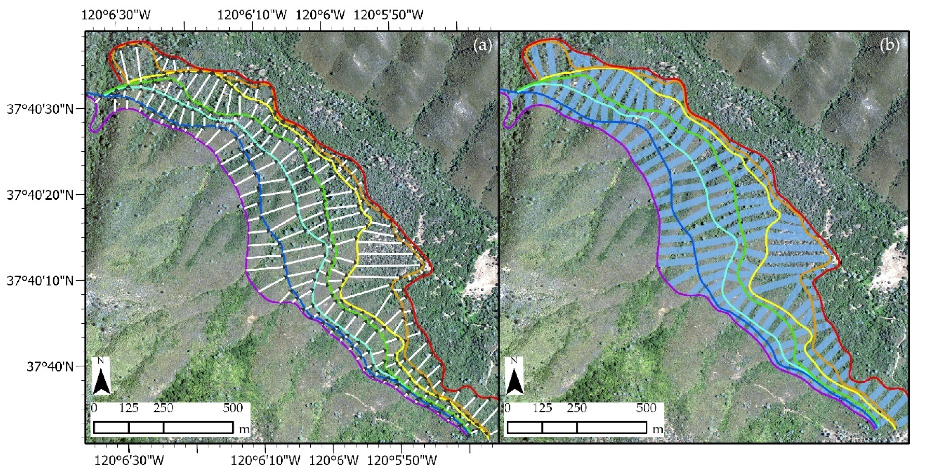
Figure 3.
Fire spread vectors and LSUs at Detwiler Fire sequence. (a) Fire spread vectors. (b) 25 m LSUs.
Figure 3.
Fire spread vectors and LSUs at Detwiler Fire sequence. (a) Fire spread vectors. (b) 25 m LSUs.


Table 1.
Linear, semi-log (exponential), log-log (power), and geographically weighted regression model diagnostics for directional slope. Separated by fire and ATIR sequence. Det. = Detwiler Fire, Th. = Thomas Fire.
Table 1.
Linear, semi-log (exponential), log-log (power), and geographically weighted regression model diagnostics for directional slope. Separated by fire and ATIR sequence. Det. = Detwiler Fire, Th. = Thomas Fire.
| Linear | Exponential | Power | GWR | ||||||||||
|---|---|---|---|---|---|---|---|---|---|---|---|---|---|
| β | Adj. R2 | p | (y = abx) | Adj. R2 | p | (y = axb) | Adj. R2 | p | β | AIC | Adj. R2 | ANOVA p | |
| Det. (n = 188) | |||||||||||||
| Vector | 0.250 | 0.160 | <0.001 | 6.650(1.031)slope | 0.075 | <0.001 | 2.200(slope)1.936 | 0.078 | <0.001 | 0.264 | 1096.48 | 0.332 | <0.001 |
| 25 m | 0.247 | 0.153 | <0.001 | 6.458(1.030)slope | 0.065 | <0.001 | 2.356(slope)1.770 | 0.067 | <0.001 | 0.262 | 1098.40 | 0.325 | <0.001 |
| 50 m | 0.262 | 0.160 | <0.001 | 6.547(1.031)slope | 0.064 | <0.001 | 2.411(slope)1.851 | 0.067 | <0.001 | 0.262 | 1098.40 | 0.325 | <0.001 |
| Th.1 (n = 361) | |||||||||||||
| Vector | 0.521 | 0.413 | <0.001 | 7.400(1.045)slope | 0.513 | <0.001 | 1.133(slope)4.979 | 0.490 | <0.001 | 0.543 | 2500.99 | 0.558 | <0.001 |
| 25 m | 0.517 | 0.423 | <0.001 | 7.379(1.046)slope | 0.505 | <0.001 | 1.129(slope)4.874 | 0.481 | <0.001 | 0.542 | 2502.71 | 0.556 | <0.001 |
| 50 m | 0.522 | 0.411 | <0.001 | 7.339(1.045)slope | 0.497 | <0.001 | 1.120(slope)4.858 | 0.472 | <0.001 | 0.548 | 2506.89 | 0.551 | <0.001 |
| Th.2 (n = 416) | |||||||||||||
| Vector | 0.459 | 0.432 | <0.001 | 6.771(1.047)slope | 0.548 | <0.001 | 0.997(slope)4.960 | 0.533 | <0.001 | 0.419 | 2812.46 | 0.582 | <0.001 |
| 25 m | 0.447 | 0.410 | <0.001 | 6.740(1.045)slope | 0.534 | <0.001 | 1.212(slope)4.639 | 0.518 | <0.001 | 0.410 | 2818.99 | 0.576 | <0.001 |
| 50 m | 0.456 | 0.423 | <0.001 | 6.681(1.048)slope | 0.518 | <0.001 | 1.311(slope)4.766 | 0.523 | <0.001 | 0.419 | 2818.54 | 0.576 | <0.001 |
| Th.3 (n = 129) | |||||||||||||
| Vector | 0.292 | 0.494 | <0.001 | 5.629(1.044)slope | 0.536 | <0.001 | 1.102(slope)3.807 | 0.513 | <0.001 | 0.309 | 743.22 | 0.551 | 0.004 |
| 25 m | 0.287 | 0.483 | <0.001 | 5.623(1.043)slope | 0.524 | <0.001 | 1.137(slope)3.753 | 0.502 | <0.001 | 0.303 | 746.62 | 0.539 | 0.005 |
| 50 m | 0.285 | 0.490 | <0.001 | 5.611(1.043)slope | 0.515 | <0.001 | 1.200(slope)3.598 | 0.491 | <0.001 | 0.302 | 750.29 | 0.526 | 0.006 |
| Th.4 (n = 377) | |||||||||||||
| Vector | 0.525 | 0.194 | <0.001 | 7.749(1.028)slope | 0.191 | <0.001 | 2.310(slope)3.028 | 0.173 | <0.0000 | 0.548 | 3083.93 | 0.342 | <0.001 |
| 25 m | 0.516 | 0.191 | <0.001 | 7.775(1.028)slope | 0.191 | <0.001 | 2.308(slope)3.031 | 0.173 | <0.0000 | 0.228 | 3088.53 | 0.334 | <0.001 |
| 50 m | 0.519 | 0.190 | <0.001 | 7.763(1.028)slope | 0.188 | <0.001 | 2.312(slope)3.006 | 0.171 | <0.0000 | 0.540 | 3088.80 | 0.334 | <0.001 |
Table 2.
Geographically weighted regression (GWR), eigenvector spatial filtering (ESF) regression, and multiple stepwise regression diagnostics.
Table 2.
Geographically weighted regression (GWR), eigenvector spatial filtering (ESF) regression, and multiple stepwise regression diagnostics.
| GWR | ESF Regression | Multiple Stepwise Regression | ||||||||||
|---|---|---|---|---|---|---|---|---|---|---|---|---|
| AIC | Adj. R2 | ANOVA p-Value | Residual SE | AIC | VIF max | Adj. R2 | p-Value | AIC | VIF max | Adj. R2 | p-Value | |
| Det. | ||||||||||||
| Vector | 1079.96 | 0.395 | 0.002 | 3.83 | 1061.95 | 6 | 0.496 | 0.013 | 1121.31 | 1 | 0.237 | <0.001 |
| 25 m | 1070.76 | 0.427 | 0.026 | 4.13 | 1082.34 | 7 | 0.414 | 0.015 | 1114.46 | 6 | 0.268 | <0.001 |
| 50 m | 1072.79 | 0.421 | 0.028 | 3.85 | 1064.59 | 9 | 0.491 | 0.016 | 1118.19 | 6 | 0.254 | <0.001 |
| Th.1 | ||||||||||||
| Vector | 2511.38 | 0.553 | <0.001 | 7.08 | 2460.93 | 7 | 0.622 | <0.001 | 2542.85 | 3 | 0.505 | <0.001 |
| 25 m | 2512.42 | 0.552 | <0.001 | 7.09 | 2463.56 | 8 | 0.621 | 0.003 | 2534.40 | 3 | 0.517 | 0.001 |
| 50 m | 2514.60 | 0.549 | <0.001 | 7.09 | 2461.52 | 8 | 0.621 | 0.005 | 2537.71 | 3 | 0.512 | 0.003 |
| Th.2 | ||||||||||||
| Vector | 2819.99 | 0.582 | <0.001 | 6.37 | 2755.96 | 8 | 0.671 | <0.001 | 2895.55 | 4 | 0.490 | 0.004 |
| 25 m | 2818.19 | 0.586 | <0.001 | 6.25 | 2744.00 | 9 | 0.651 | 0.002 | 2886.62 | 5 | 0.501 | 0.004 |
| 50 m | 2805.79 | 0.596 | <0.001 | 6.26 | 2749.32 | 9 | 0.649 | 0.003 | 2882.78 | 5 | 0.504 | 0.006 |
| Th.3 | ||||||||||||
| Vector | 738.28 | 0.577 | 0.015 | 3.443 | 704.54 | 1 | 0.706 | <0.001 | 747.61 | 1 | 0.543 | <0.001 |
| 25 m | 740.76 | 0.568 | 0.010 | 3.604 | 710.29 | 3 | 0.677 | <0.001 | 751.20 | 1 | 0.531 | <0.001 |
| 50 m | 748.47 | 0.542 | 0.019 | 3.605 | 708.27 | 4 | 0.675 | 0.002 | 757.16 | 1 | 0.508 | <0.001 |
| Th.4 | ||||||||||||
| Vector | 3083.91 | 0.354 | <0.001 | 12.93 | 2018.33 | 4 | 0.463 | <0.001 | 3133.22 | 4 | 0.251 | <0.001 |
| 25 m | 3124.03 | 0.267 | <0.001 | 12.86 | 2013.11 | 5 | 0.469 | <0.001 | 3124.03 | 5 | 0.269 | <0.001 |
| 50 m | 3069.48 | 0.381 | <0.001 | 12.66 | 2002.61 | 5 | 0.485 | <0.001 | 3119.65 | 7 | 0.277 | <0.001 |
Table 3.
Residual Moran’s I of 50 m LSU models for stepwise regression and ESF regression.
| Stepwise | ESF | |||
|---|---|---|---|---|
| 50 m LSU Model | Moran’s I | p-Value | Moran’s I | p-Value |
| Detwiler | 0.445 | <0.001 | −0.068 | 0.659 |
| Thomas 1 | 0.372 | <0.001 | 0.057 | 0.732 |
| Thomas 2 | 0.388 | <0.001 | −0.059 | 0.806 |
| Thomas 3 | 0.441 | <0.001 | −0.073 | 0.630 |
| Thomas 4 | 0.350 | <0.001 | −0.033 | 0.745 |
Table 4.
Stepwise (b1) and ESF (b2) regression coefficient comparison of vector LSU models. Dashes (—) indicate an insignificant variable in the model.
Table 4.
Stepwise (b1) and ESF (b2) regression coefficient comparison of vector LSU models. Dashes (—) indicate an insignificant variable in the model.
| Stepwise (β1) and Moran’s I Eigenvector Spatial Filtering (β2) Regression Coefficients | ||||||||||
|---|---|---|---|---|---|---|---|---|---|---|
| Spread Sequence | ||||||||||
| Detwiler | Th.1 | Th.2 | Th.3 | Th.4 | ||||||
| β1 | β2 | β1 | β2 | β1 | β2 | β1 | β2 | β1 | β2 | |
| Directional Slope | 0.26 | 0.27 | 0.53 | 0.53 | 0.45 | 0.41 | 0.38 | 0.27 | 0.56 | 0.49 |
| Shrub Fraction | — | — | — | — | — | — | 3.16 | 3.98 | — | — |
| Herb Fraction | 4.35 | 3.94 | 19.87 | 7.11 | 9.43 | 9.05 | — | — | — | — |
| Tree Fraction | — | — | −14.55 | −25.58 | — | — | — | — | −29.06 | −22.86 |
| Rock/Barren Fraction | — | — | — | — | −9.39 | −7.05 | — | — | −21.92 | −22.81 |
| NDVI | — | — | 19.67 | 11.40 | 40.22 | 23.02 | 18.19 | 14.00 | 51.79 | 81.88 |
| GRVI | — | — | −98.11 | 104.56 | −102.91 | −69.41 | — | — | — | — |
| NDRB | — | — | — | — | — | — | — | — | — | — |
Table 5.
Machine learning model diagnostics. Cross validation (CV) statistics are leave-one-out (LOO).
Table 5.
Machine learning model diagnostics. Cross validation (CV) statistics are leave-one-out (LOO).
| CART (Regression Tree) | Random Forest | |||||
|---|---|---|---|---|---|---|
| CV RMSE | CV R2 | Variables Required by Model | CV RMSE | CV R2 | Variable Importance (Top 3) | |
| Det. | ||||||
| Vector | 4.60 | 0.396 | slope, herb, shrub, NDVI | 4.49 | 0.322 | slope, herb, shrub |
| 25 m | 4.74 | .399 | slope, herb, shrub, GRVI | 4.61 | 0.336 | slope, herb, shrub |
| 50 m | 4.83 | .391 | slope, herb, shrub, GRVI | 4.81 | 0.313 | slope, herb, shrub |
| Th. 1 | ||||||
| Vector | 7.48 | 0.602 | Slope, herb, GRVI, NDRB | 7.19 | 0.643 | slope, shrub, GRVI |
| 25 m | 7.26 | 0.620 | Slope, shrub, herb, GRVI, NDRB | 6.94 | 0.650 | slope, shrub, herb |
| 50 m | 7.48 | 0.606 | Slope, shrub, herb, GRVI, NDRB | 7.14 | 0.643 | slope, shrub, herb |
| Th.2 | ||||||
| Vector | 6.79 | 0.623 | slope, herb, rock and barren, NDVI | 6.58 | 0.657 | slope, herb, rock and barren |
| 25 m | 6.99 | 0.604 | slope, herb, rock and barren, NDVI | 6.73 | 0.639 | slope, herb, rock and barren |
| 50 m | 7.07 | 0.596 | slope, herb, rock and barren, NDVI | 6.82 | 0.631 | slope, herb, NDVI |
| Th.3 | ||||||
| Vector | 3.80 | 0.670 | slope, shrub, NDVI, GRVI | 3.52 | 0.667 | slope, shrub, NDVI |
| 25 m | 3.64 | 0.711 | slope, rock and barren, shrub, NDVI, GRVI | 3.42 | 0.721 | slope, shrub, rock and barren |
| 50 m | 4.05 | 0.692 | slope, shrub, herb, NDVI | 3.84 | 0.717 | slope, shrub, herb |
| Th.4 | ||||||
| Vector | 12.31 | 0.508 | slope, shrub, rock and barren, NDVI, GRVI | 11.40 | 0.551 | slope, shrub, rock and barren |
| 25 m | 11.01 | 0.544 | slope, shrub, rock and barren, NDVI, GRVI | 10.61 | 0.563 | slope, shrub, rock and barren |
| 50 m | 12.89 | 0.442 | slope, shrub, rock and barren, NDVI, GRVI | 12.69 | 0.458 | slope, shrub, rock and barren |
Publisher’s Note: MDPI stays neutral with regard to jurisdictional claims in published maps and institutional affiliations. |
© 2022 by the authors. Licensee MDPI, Basel, Switzerland. This article is an open access article distributed under the terms and conditions of the Creative Commons Attribution (CC BY) license (https://creativecommons.org/licenses/by/4.0/).
Share and Cite
MDPI and ACS Style
Schag, G.M.; Stow, D.A.; Riggan, P.J.; Nara, A. Spatial-Statistical Analysis of Landscape-Level Wildfire Rate of Spread. Remote Sens. 2022, 14, 3980. https://doi.org/10.3390/rs14163980
AMA Style
Schag GM, Stow DA, Riggan PJ, Nara A. Spatial-Statistical Analysis of Landscape-Level Wildfire Rate of Spread. Remote Sensing. 2022; 14(16):3980. https://doi.org/10.3390/rs14163980
Chicago/Turabian StyleSchag, Gavin M., Douglas A. Stow, Philip J. Riggan, and Atsushi Nara. 2022. "Spatial-Statistical Analysis of Landscape-Level Wildfire Rate of Spread" Remote Sensing 14, no. 16: 3980. https://doi.org/10.3390/rs14163980
Note that from the first issue of 2016, this journal uses article numbers instead of page numbers. See further details here.