
LCNS Positioning of a Lunar Surface Rover Using a DEM-Based Altitude Constraint
by
 , and
, and
Floor Thomas Melman
1,* ,
,
Paolo Zoccarato
1,
Csilla Orgel
1,
Richard Swinden
1,
Pietro Giordano
1 and
Javier Ventura-Traveset
2 1
European Space Research and Technology Centre (ESTEC), European Space Agency, Keplerlaan 1, P.O. Box 299, 2200 AG Noordwijk, The Netherlands
2
Centre Spacial de Toulouse, European Space Agency, 18 Avenue Edouard Belin, CEDEX 9, 31401 Toulouse, France
*
Author to whom correspondence should be addressed.
Remote Sens. 2022, 14(16), 3942; https://doi.org/10.3390/rs14163942
Submission received: 28 June 2022
/
Revised: 7 August 2022
/
Accepted: 10 August 2022
/
Published: 14 August 2022
(This article belongs to the Special Issue Autonomous Space Navigation)
Abstract
:With the renewed interest in lunar surface exploration, the European Space Agency envisions to stimulate the creation of lunar communications and navigation services (LCNS) to enable, among others, autonomous navigation capabilities for lunar rovers. As the number of satellites foreseen in such a service is much smaller compared to Earth-based global navigation satellite systems, different complementary technologies are pursued to improve the attainable navigation accuracy for lunar rovers. One way to improve the position accuracy provided by the LCNS satellites is to constrain their vertical position using a high resolution digital elevation model (DEM). This article presents the results of a variance covariance analysis of an extended Kalman filter implementation in which the LCNS ranging measurements are used together with the altitude provided by a DEM from the Lunar Orbiter Laser Altimeter instrument of the Lunar Reconnaissance Orbiter. Assuming a realistic orbit determination and time synchronization accuracy of the LCNS satellites, the usage of a navigation-grade inertial measurement unit and an oven-controlled crystal oscillator, a 3-sigma position accuracy of less than 10 m can be obtained. Furthermore, the availability is substantially improved as the DEM-aided solution enables a position solution in case of only 3 visible satellites.
1. Introduction
The interest in lunar exploration has grown significantly in the past few years, both at the institutional and commercial levels [1]. The Earth-based techniques currently adopted for communication and navigation with satellites in cislunar space are not able to cover all the needs for future exploration, both in terms of service accessibility (the South Pole and the far side are not always accessible by Earth-based ground stations) and service performance (i.e., need to land within 100 m of a predetermined location on the lunar surface [2]). The European Space Agency’s (ESA) vision, represented in the Moonlight initiative [3], is to stimulate the creation and development of lunar communication and navigation services (LCNS), to be delivered by private partners, that will support the next generation of institutional and private lunar exploration missions, including the enhancement of the performance for those missions currently under definition.
Several other space agencies and commercial entities have proposed dedicated systems to offer communication and navigation services within the (cis)lunar service volume. In the US, Lockheed Martin has proposed Parsec [4]. JAXA (Japan Aerospace Exploration Agency) has recently launched a study which will consider possible lunar positioning satellite systems [5]. Roscosmos has announced a concept that envisions the deployment of a lunar satellite navigation system between 2036 and 2040 [6]. Finally, China recently announced that its space agency (CNSA) is planning to set up a satellite constellation around the Moon to provide communication and navigation services [7]. On top of these initiatives, NASA has proposed the LunaNet framework to enable interoperability among different lunar communication and navigation service providers [8].
The challenge of accurate navigation for lunar surface users (i.e., rovers) has been of interest since the early robotic explorations of the Moon [9] and typically relies on technologies such as dead-reckoning, using, among others, inertial navigation systems (INS) [10], wheel odometry and visual odometry (VO) [11,12,13] for terrain relative localization. The advantage of visual navigation is its passive nature [14] (as it uses visual light) and the imagery can be used for hazard avoidance and traverse planning [15]. Dead-reckoning technologies, however, are not suitable for long traverses as the error grows without bounds [16]. For absolute positioning, planetary rovers relied on “ground-in-the-loop” processing of down-link images in which on-board images where interactively registered (i.e., mapping between local and global maps) to orbital imagery [17]. Such an approach, however, is impractical for autonomously operated vehicles. Furthermore, the attainable absolute accuracy is determined by the resolution of the global (orbital) maps [18]. Nevertheless, recent developments may allow autonomous processing and registering of global and local imagery or 3D point clouds [15].
Rover images can also be used to derive local digital elevation models (DEM). When the global DEMs are available on-board the rover, they can be correlated against local DEMs to provide a global position [19]. However, variation in the solar illumination angle may lead to a change in the terrain appearance which complicates the image registration [17]. LIDAR (light detection and ranging) can be used to remove the dependency on surface illumination conditions [16]. Tests on Earth in a Mars-Moon analogue environment when using 3D LIDAR scans for matching against a 3D orbital map for global navigation (complemented by visual odometry and an inclinometer/Sun-sensor) resulted in position errors smaller than 100 m [16]. Finally, craters can be used as landmarks to yield a global navigation solution [17] obtaining high positioning accuracies (5 to 10 m). Nevertheless, the position accuracy is determined by, among other things, the size of the crater and illumination conditions.
Alternatively, rovers can use radio frequency (RF) tracking techniques [20]. Current radiometric tracking of surface users relies mostly on a direct-to-Earth link, which has some intrinsic limitations. First of all is the impossibility to serve far-side missions. In addition, serving one user at a time substantially limits the autonomy of assets on the lunar surface. To overcome this issue, several studies have considered dedicated lunar navigation systems [18,20,21] consisting of 1 or 2 satellites (potentially complemented by a pseudolite or reference station on the lunar surface) to augment the previously (e.g., visual odometry) mentioned technologies. As demonstrated in [18], using a joint Doppler and ranging approach, a relative (with respect to a reference station) positioning accuracy of 10–15 m can be obtained using 2 satellites and a surface beacon. An absolute accuracy of 100 m can be obtained globally after processing 2 h of observations. The LiASON (Linked Autonomous Interplanetary Satellite Orbit Navigation) concept exploits inter-satellite link range and range-rate data to compute relative and inertial absolute positioning, obtaining a navigation accuracy of 150 m (1-sigma) using the inter-satellite links alone. When adding 4 h of daily DSN (deep space network) observations, a navigation positioning accuracy on the order of 10 m can be achieved [21].
A dedicated LCNS, such as the one proposed within the ESA’s Moonlight initiative, would provide several advantages over the previously mentioned technologies. First of all, its performance is not dependent on illumination conditions. This is important as rovers may need to traverse permanently shadowed regions on the lunar South Pole [22] as these may contain water ice [23]. Secondly, it would improve the autonomy of the rover as it passively uses the LCNS signals in one-way ranging mode (i.e., it will not actively use resources of the LCNS satellites for navigation purposes). Thirdly, the navigation accuracy is not governed by the size and shape of features that are used to register local and global maps. Finally, the positioning accuracy is only marginally impacted by the accuracy of available maps (e.g., DEMs and feature maps).
This paper presents the results of a covariance analysis covering the navigation performances achievable by a lunar rover using the Moonlight navigation service as received by a Moonlight user together with inertial measurement units (IMU) and DEM information. This contribution considers a lunar traverse covering the South Pole. The considered algorithm is based on an extended Kalman filter (EKF) in which the altitude is constrained (with respect to the lunar ellipsoid) by the DEM available onboard the rover, allowing for complete autonomy from ground operations. This not only improves the accuracy of the rover position but also enables the rover to compute its position using only 3 satellites (contrary to the 4 satellites that are typically required for terrestrial global navigation satellite systems (GNSS) receivers), thereby improving the availability of the LCNS service.
The uncertainty of the DEM is monitored considering the uncertainty of the DEM (due to interpolation and orbital errors) and the uncertainty of the rover position (which can result in a large altitude uncertainty near the edge of a crater). Thanks to detailed maps generated by the measurements performed by the LOLA (Lunar Orbiter Laser Altimeter) instrument [24] flying in the Lunar Reconnaissance Orbiter (LRO) [25], DEMs are available covering the South Pole at a resolution of 5 m per pixel and a geolocation uncertainty of 10–20 cm horizontally and 2–4 cm vertically [26].
This paper is structured as follows. Section 2 provides an overview of the lunar rover traverse used and its characteristics. Section 3 describes the LCNS constellation considered in this publication as well as the characteristics of the rover, including the satellite orbits, payload characteristics and rover receiver. Section 4 addresses the mathematical formulation of the covariance analysis. Section 5 reports the results of the simulations, and Section 6 provides the conclusive remarks.
2. Lunar Surface Rover Mission Profile
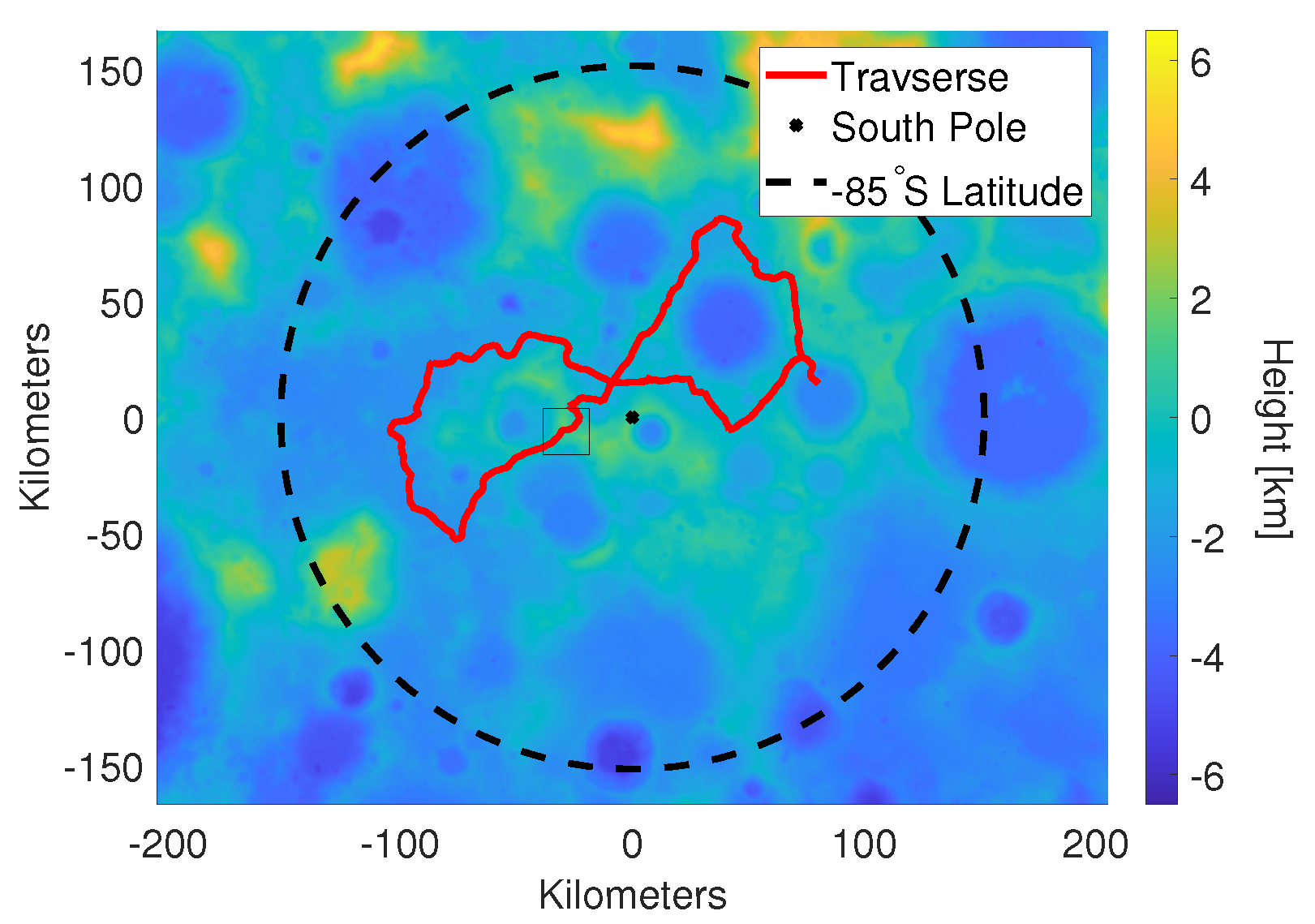
The rover traverse selected for this paper is based on the literature [22] and circumnavigates the de Gerlache crater in an anti-clockwise direction (see Figure 1). With a total length of 320 km, expected to be covered in about 11 days by a pressurized rover with an average speed of 5 km/h (operated by humans) [22], this traverse has been chosen to cover areas of scientific interest and present two major technical advantages: first, the slopes encountered in the traverse are manageable by the actual rovers (i.e., lower than 25 degrees), and second, the traverse is covered by high-resolution DEMs. This paper only considers a small portion of this traverse, which coincides with one of the high-resolution lunar DEMs [26]. The portion of the traverse considered in this publication is highlighted in Figure 1 with a black square. From this point forward, the term “traverse” is used to refer to this small portion of the overall traverse proposed in [22].
A remotely operated rover was chosen for this study, with a maximum speed of 0.36 km/h [22] (which is representative of tele-robotic operation), contrary to the 5 km/h which was considered by [22] for a small pressurized rover (SPR), leading to a completion of the traverse portion (as bounded by the black squared in Figure 1) in about 3 days. The two-dimensional traverse was converted to a three-dimensional traverse sampled at a rate of 1 Hz by considering a maximum horizontal velocity of 0.36 km/h using the following steps:
- Loading the 2D traverse [22] provided in a replaced[id=fm]geographic information systemGeographic Information System (GIS) shapefile;
- Time tagging the points along the traverse such that the horizontal velocity equals 0.36 km/h;
- Interpolating the horizontal traverse at the requested time-step (1 s);
- Interpolating the DEM to get the rover position in polar stereograhic reference frame (including the height). As the velocity is horizontally constrained, the actual velocity in three dimensions will be slightly larger than 0.36 km/h;
- Converting the polar stereographic coordinates to a selenodetic reference frame.
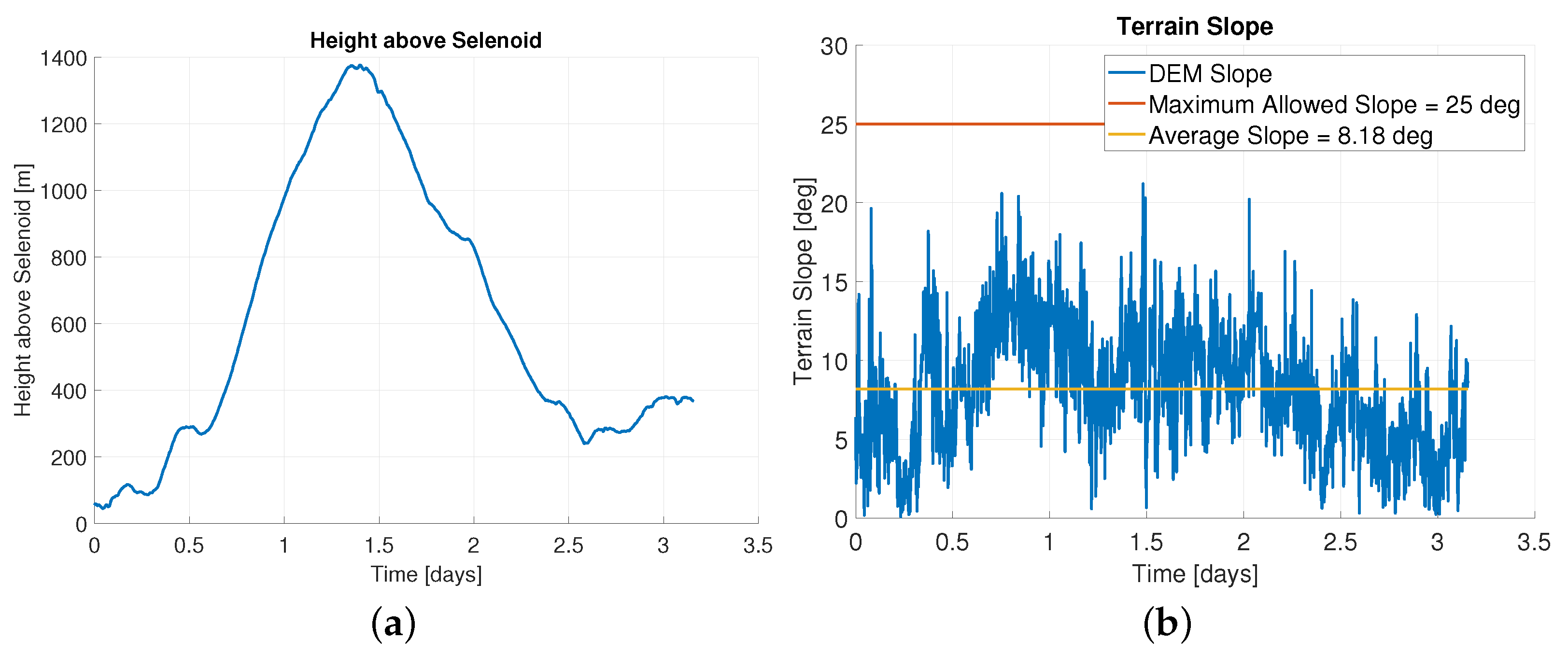
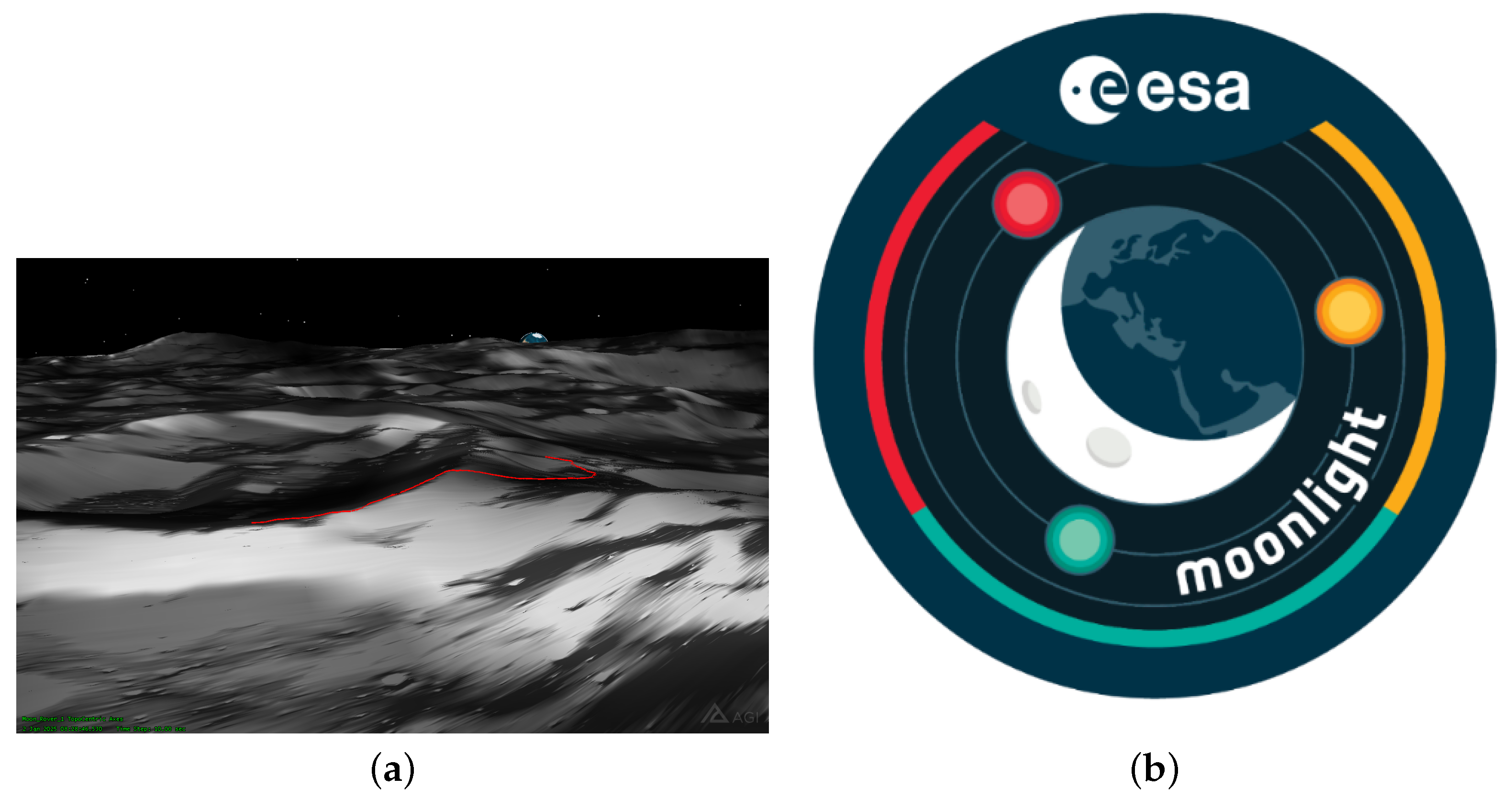
Figure 2 shows the elevation and slope along the traverse with the time in days covering a distance of approximately 27 km and a height ascent of 1300 m. The maximum slope encountered is 21.2 degrees, while the average slope is 8.2 degrees. The traverse was loaded into the ESA lunar navigation simulator [28,29] to acquire the link data with the LCNS satellites. The simulation environment used in the publication also considered the terrain data provided on the NASA PDS archive and generated by LOLA [27]. In this way, the simulation also accounts for the local topography and related signal occultations (see Figure 3a for the implementation of the traverse in the simulation environment).
3. Moonlight and LCNS
The Moonlight navigation service (see Figure 3b for the mission logo) aims to provide a one-way broadcast radio navigation signal to allow a user to compute its position, velocity and time, similarly as done for GNSS (e.g., the signals broadcasted by the Moonlight satellites will be synchronized among them). This concept has been presented in the past (e.g., [30]), but now Moonlight can take advantage of the significant evolution of GNSS technologies both at the satellite/system and user levels. In fact, the Moonlight navigation concept aims to extensively and intentionally reuse GNSS technology in order to achieve fast time-to-market (the current target is to provide the first services in the 2027–2028 time frame) and ease the introduction of the concept within future lunar missions by means of reuse of already existing spaceborne GNSS receivers with minimum modifications. This is achieved by implementing GNSS modulations, navigation techniques and technologies. This concept has been embraced by the NASA LunaNet framework and called lunar augment navigation services (LANS) [8].
ESA defined 3 phases to establish a lunar radio navigation service:
- Phase 1–Use of High-Sensitivity Space Receivers (2022–2025): Based on the reception of Earth GNSS signals with high-sensitivity receivers, on-board dynamic filters and high-gain antennas. This phase should provide initial services for Earth-Moon transfers and lunar orbit operations.
- Phase 2–Lunar Communication and Navigation Services (LCNS) (2025–2035): Enhancing the Phase 1 with the transmission of additional ranging signals from both the Moon orbit and surface. This phase should allow a major reduction of the geometric DOP (dilution of precision) and improve the service availability, which, in turn, would translate into enhanced lunar orbit navigation and initial landing/surface PNT (position, navigation and timing) services (e.g., on the Moon’s South Pole).
- Phase 3–Full Lunar PNT System (2035-onwards): This phase should provide PNT services on the whole Moon surface and enhance the positioning availability and accuracy in the Moon orbit and on the lunar South Pole. This could be obtained by complementing Phase 2 with additional lunar orbiting satellites and Moon surface beacons. This phase could also allow for the provision of integrity services for safety critical applications, leading to increased autonomy.
This contribution focuses on how Phase 2 (LCNS) could support rover surface operations.
Two parallel Phase A/B1 studies are ongoing at the moment to define the Moonlight system; therefore, this contribution does not aim to provide the definitive constellation or characteristics, but rather to provide an example of what can be achieved with such a system. The results provided in this contribution are considered representative of the future system, even if the actual constellation might not be identical to the one used here.
As mentioned in previous publications [29,31,32], at least during Phase 2 of the Moonlight navigation roadmap, the navigation service will not be able to serve users in every location all the time. Given the limited number of satellites on the initial LCNS constellation (see Section 3.1), the navigation service will be provided in specific time slots for a specific area of the lunar surface. For this reason, user mission analysts will have to plan the critical operations (e.g., final descent of a lunar lander) based on the predicted availability of the service. This process has been described in details in [29,32], and it is used accordingly in this contribution.
3.1. LCNS Constellation
The LCNS constellation considered in this paper is comprised of four satellites in elliptical lunar frozen orbits (ELFO). These orbits are highly eccentric and have their argument of perilune (i.e., the point at which the spacecraft in lunar orbit is closest to the Moon) close to the Moon’s North Pole to ensure maximum coverage above the Moon’s South Pole. The four satellites are located in two different planes, wherein the satellites in the first plane are separated by 123.4, and the satellites in the second plane are separated by 180. The orbital parameters are provided in Table 1.
The constellation parameters in this publication have been derived by ESA based on internal studies, but these may be further optimised. Better performances are indeed expected with the constellation provided in the Phase A/B1 studies currently ongoing.
3.2. LCNS Payload
The navigation payload in the LCNS satellites is responsible for broadcasting one-way ranging signals to the lunar users. Contrary to the Earth, the Moon does not have a significant atmosphere, removing the need for dual-frequency broadcasting. Furthermore, to avoid potential interference with Earth GNSS L-band signals (which may be used up to Lunar altitudes [28]) and in line with the Space Frequency Coordination Group (SFCG)’s R32 recommendation [33], the signals are transmitted using the S-band carrier frequency (2491.005 MHz). Finally, to keep the receiver implementation simple (note that lunar users may use both LCNS and Earth GNSS), a simple BPSK(5) (binary phase shift keying) modulation is used (similarly to the Galileo E6BC signal). The signal characteristics are summarized in Table 2.
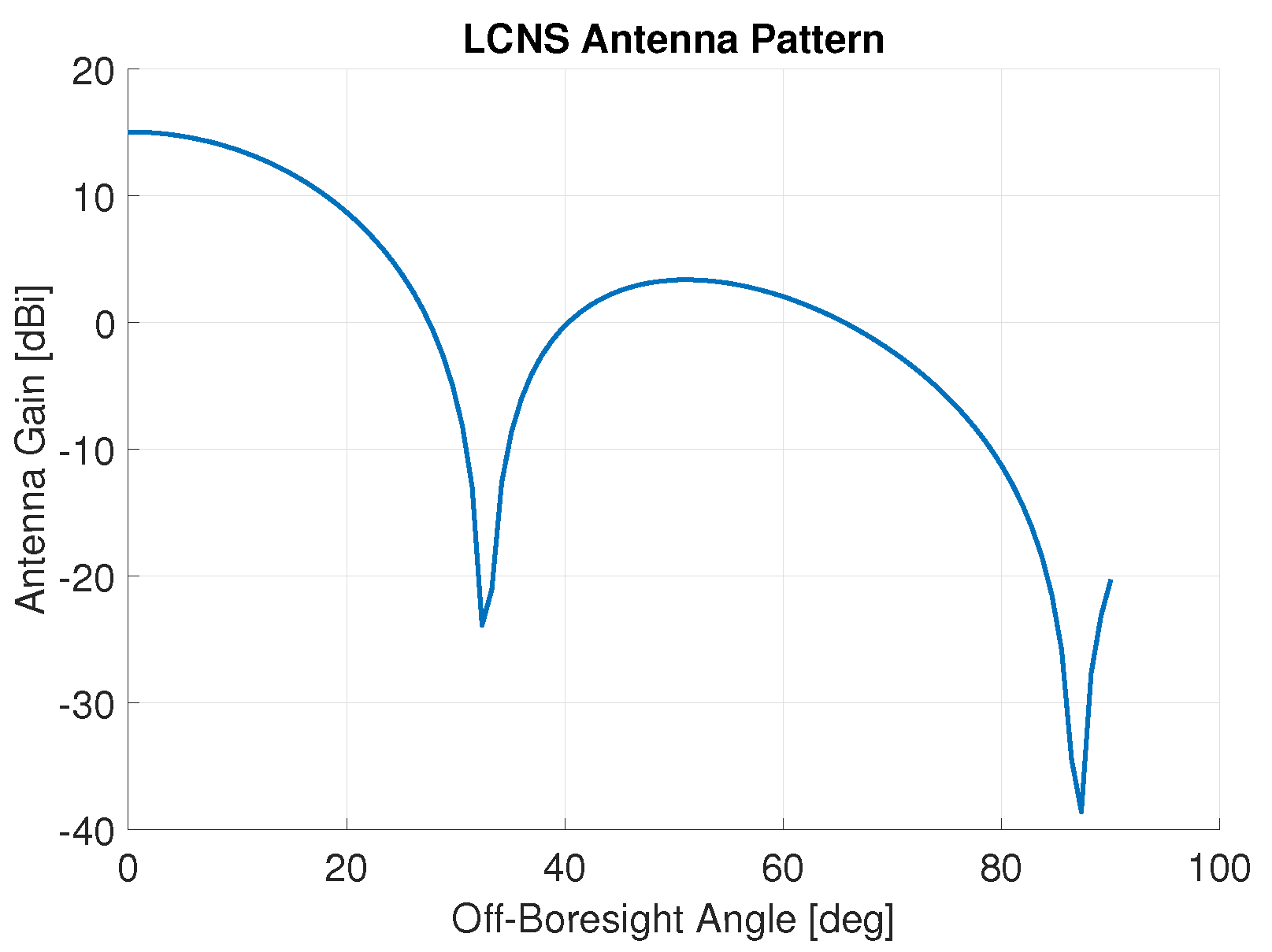
The LCNS antenna boresight is pointed towards the centre of the Moon (i.e., nadir-pointing). As the distance between the surface and the Moon and the LCNS satellites is relatively small (compared to the Earth GNSS case), the EIRP (effective isotropic radiated power) can be kept small and is considered to be 15.02 dBW at boresight. The LCNS transmission antenna pattern is considered symmetric, and the off-boresight EIRP is provided in Figure 4. The transmission antenna pattern considered in this publication is based on internal ESA studies and aims to provide an example of a more representative pattern compared to previous publications from the same authors [29,32,34]. It is important to note that the final antenna patterns for LCNS are currently under assessment within the Phase A/B1 studies and are expected to be provide similar (or better) performances.
3.3. Rover LCNS Receiver
In line with previous works [29,32], the lunar surface rover will be equipped with a LCNS receiver, which can be modelled similarly to a space-borne GNSS receiver. Such a receiver is comprised of a radio frequency front-end (RFFE) and digital parts for signal processing. The main difference with respect to a GNSS receiver will be the change of carrier frequency from the L-band to S-band; the rest will be almost identical.
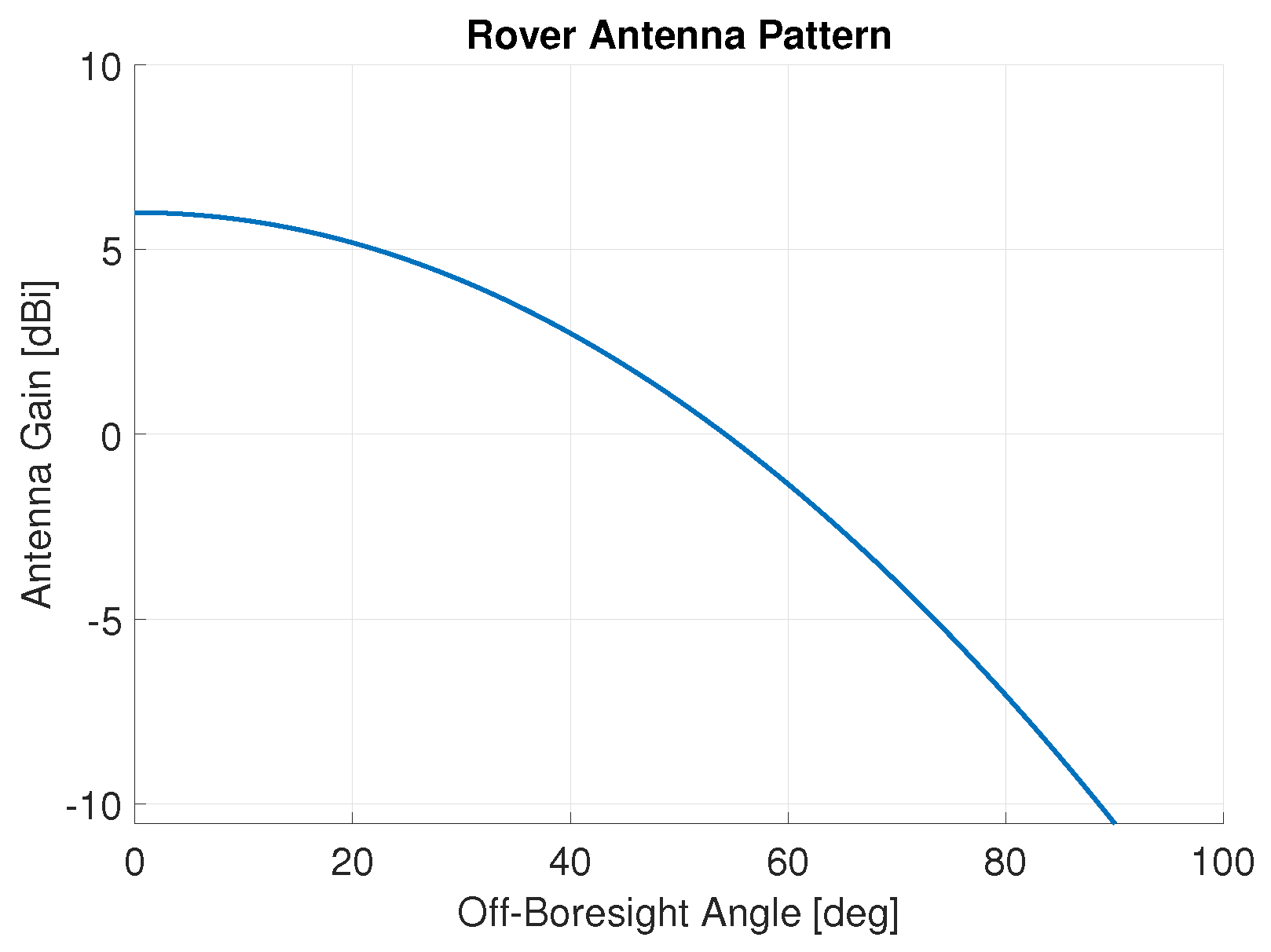
The carrier-to-noise-density ratio () as seen by the receiver is modelled using Equation (1) [35]. The is defined above and set to 15.02 dBW at boresight, represents the free space loss, the atmospheric losses (which should be negligible in case of the Moon), represents the receiver gain (as shown in Figure 5), k represents Boltzmann’s constant and represents the equivalent noise temperature (which is defined in Table 3).
The receiver is expected to rely on state-of-the-art tracking techniques using a DLL (delay locked loop) and PLL (phase locked loop). Within the simulation environment used in this contribution. a hard acquisition and a (carrier-to-noise density ratio) tracking threshold at 30 dB-Hz was selected (in line with [29]). Any signal with a below this threshold was considered not acquired nor tracked. This is an arbitrary decision that will be revisited as part of Phase A/B1 and that drives the overall link budget and payload EIRP. For the scope of this publication, the threshold is considered achievable with current state-of-the-art technology at the user level assuming the receiver implements high-sensitivity techniques to allow the tracking of a BPSK(5)-like signal below 32 dB-Hz [36]. This assumption is expected to have limited impact on the attainable positioning accuracy, as the measurement accuracy is mostly driven by the orbit determination and time synchronization (ODTS) accuracy. However, it may impact the number of satellites that are available for positioning. Furthermore, the RFFE noise figure has been set to 1 dB, which should be in line with state-of-the-art products for space applications [29]. Finally, the noise temperature is set to 113 K (based on an internal ESA assessment; this value will be re-assessed in future publications) and the LNA (low noise amplifier) gain to 30 dB. All receiver parameters are summarized in Table 3.
The antenna of the rover is assumed to be pointing in the zenith direction (i.e., upwards). This assumes an ideal case when the rover moves on a flat surface. In reality, the direction the antenna points will vary with the slope of the local terrain. The impact of this assumption, however, is considered small (i.e., note a gain variation of 1 dBi in Figure 5 between the zenith and an off-boresight angle of 20 degrees). The receiver antenna is assumed to be symmetric in the azimuth, and the elevation pattern is visualized in Figure 5, which is considered representative of what is currently available on the market for space-borne GNSS antennas. Similar performances are achievable in the S-band. No elevation mask is implemented; however, lunar terrain in the vicinity of the traverse (refer to Section 2) was considered to evaluate the impact of the local topography on the visibility between the rover and the LCNS satellites.
The navigation system of the LCNS receiver will be complemented by an inertial measurement unit (IMU). Within this study, a tactical grade IMU similar to LN200S [37] is considered, which has been used by the most recent NASA Mars rovers (i.e., Spirit, Opportunity, Curiosity and Perseverance). Within this study, the impact of the IMU is not directly modelled; however, its contribution is accounted for in the definition of the process noise of the EKF (for more details refer to Section 4 or previous publications [29]). Table 4 provides examples of the characteristics of different grades of IMUs. The process noise indicated in Table 4 will be used to define the process noise in the simulation, as further detailed in Section 4.4.

Table 4.
Examples of different types of space-grade IMUs and their characteristics. Note that the velocity process noise considers a conservative integration time of 1 s.
Table 4.
Examples of different types of space-grade IMUs and their characteristics. Note that the velocity process noise considers a conservative integration time of 1 s.
| Navigation Grade | Tactical Grade | |
|---|---|---|
| Weight | 9.0 kg | 748 g |
| Example | iMAR iNAV-RQH-1001 [38] | Northtrop Grumman LN-200S [37] |
| Velocity Random Walk | 8 μg/ | 35 g/ |
| Velocity Process Noise () | 7.8 m/s/ | 3.4 m/s/ |
The clock of the navigation receiver is expected to be an oven-controlled crystal oscillator (OCXO). The characteristics of such a clock type and its impact on the process noise can be found in Table 5. The process noise indicated in Table 5 will be used to define the process noise in the simulation, as further detailed in Section 4.4.
Table 5.
Examples of space grade OCXO clocks.
| Product | Microchip OX-249 [39] | AXTAL AXIOM6060 [40] | AXTAL AXIOM70SL [41] |
|---|---|---|---|
| Weight | 14 g | 200 g | 20 g |
| Reference frequency | n/a | 100 MHz | 10 MHz |
| Frequency Stability | 100 ppb | 50 ppb | 10 ppb |
| Allan Deviation ( = 1 s) | |||
| Clock Bias Process Noise () | 0.003 m/ | 0.030 m/ | 0.001 m/ |
| Clock Drift Process Noise () | 30 m/s/ | 15 m/s/ | 3 m/s/ |
4. Covariance Analysis
4.1. Extended Kalman Filter
The positioning engine in the LCNS receiver will implement an EKF. Similar to surface users on Earth, the estimation is kinematic (i.e., the position is propagated only by the velocity). In this contribution, a variance-covariance analysis is employed, meaning that the states are not actually estimated, but only the effect of the measurement errors and geometry on the EKF solution is assessed; therefore, only the implemented EKF equations regarding the propagation and update from measurements of the state covariance matrix are described. For further details regarding the EKF and its derivation, the reader is referred to the existing literature [42,43].
The state vector estimate can be propagated forward to an epoch k by the relationship in Equation (2), where is the predicted state at epoch k, and denotes the state transition matrix from epoch to k.
The state estimate covariance matrix can be propagated to an epoch k by the relationship in Equation (3), where is the predicted state covariance matrix at epoch k, is the process noise transition matrix, (positive semi-definite ) is the process noise covariance matrix and denotes the transpose operator. In real operations, the initial covariance will be estimated using the weighted least squares (WLS) algorithm. In this paper, however, we assume a fixed value for , which is further detailed in Section 4.4.
The equations that are used to propagate and predict the covariance of the state vector are given below.
The state vector contains 8 elements and is given in Equation (4), where denotes the 3D position vector in a Moon fixed reference frame, denotes the 3D velocity, denotes the receiver clock bias and denotes the receiver clock drift.
It is assumed that measurements are available at epoch k in the form described by Equation (5), where denotes the design (or measurement) matrix (which is defined in Section 4.3), and denotes the measurement noise, assumed to be zero-mean and with covariance matrix (which is defined in Section 4.5).
Equation (6) shows the definition of the Kalman gain matrix.
Equation (7) shows the definition of the state covariance update step using the Bucy–Jopseh formulation (note that I denotes the 8 × 8 identity matrix). This formulation has been selected as it ensures is symmetric.
4.2. Prediction Model
The prediction model is selected in alignment with previous works [29] and represents the dynamics of the lunar rover. As previously discussed in Section 4.1, a simple kinematic model was selected assuming a uniform motion such that the propagation of the rover position at epoch k is based on the estimation of its velocity at epoch . The state transition matrix (or propagation model) is shown in Equation (8), with the identity matrix and the length of the time interval between epochs and k.
Whereas the state transition matrix assumes a linear motion profile, the motion of the rover will be non-uniform. This mismodelling is considered in the propagation step by adding additional uncertainty by means of the process noise matrix , which is defined in Equation (9), where , , and are the process noises associated, respectively, with the user position, velocity, clock bias and clock drift elements in the state vector.
To account for the length of the propagation time-step (), the process noise transition matrix , as defined in Equation (10), is used.
In this contribution, however, the propagation time-step is considered to be 1 s, such that .
The definition of the process noise plays an important role in the final accuracy that can be achieved. Therefore, this paper performs a sensitivity study using different process noise values to assess the impact on the attainable position accuracy.
4.3. Measurement Model
The mathematical model for the covariance analysis adapted in this paper is based on previous works [29] (to which the reader is referred for a full derivation). The design matrix is repeated here and completed with the DEM measurement for completeness in Equation (11), in which represents the Euclidean norm, represents the distance from the rover to LCNS satellite m, represents the distance from the centre of the Moon to the rover given by the DEM and represents a 3 × 1 column vector containing zeroes.
Note that this model represents the case where at least 4 satellites are visible such that the rank of the design matrix is equal to or larger than the number of states. However, in case only 3 satellites are visible and 1 DEM measurement is available, the rank of the design matrix is 7, while the number of states is equal to 8 (note that a DEM range-rate measurement would not be realistic as the DEM resolution is 5 m per pixel and the rover moves at a velocity of 0.1 m per second). Therefore, in the case of 3 available satellites, the LCNS range-rate measurements are disabled, meaning in Equation (11) is removed. In such a case, only position is estimated directly, while the velocity of the rover is propagated through the dynamical model.
4.4. Simulation Settings
Table 6 shows the main configuration settings for the covariance analysis grouped in three sets of parameters: LCNS ODTS uncertainty (which drives the SISE—signal in space error), the EKF process noise (which drives the definition of the process noise matrix Q defined in Equation (9)) and the initial state covariance of the EKF (which defines ).
The ODTS uncertainty was selected to be in line with the parameters provided by previous work [29,32], which are considered achievable at maximum age-of-data (AOD) (AOD was defined in line with the Galileo Service Definition Document (SDD) [44]). This parameter represents the system contribution to the user ranging error (also known as user equivalent range error, UERE). In this study, the ODTS uncertainty was considered to be the same in each direction (i.e., radial, tangential and along-track), and therefore, the uncertainties provided in Table 6 were directly mapped to the line-of-sight. This is clearly a simplification that aims to provide an upper bound of the performances. Two parallel studies to gain more insight into the ODTS uncertainty that can be achieved for a lunar navigation system are currently running at ESA. The outcomes of these studies will be taken into account in further studies to allow for a more realistic estimation of the SISE.
Similarly to the ODTS uncertainty, the EKF process noise was selected to be in line with previous works [29,32]. However, the magnitude of the clock process noise was adapted, and a higher process noise was associated with the clock drift (as this parameter drives the propagation of the clock bias). Furthermore, in this publication, the process noise related to the clock bias and drift was driven by the Allan deviation and frequency stability, respectively, assuming an OCXO (details on the Allan deviation and frequency stability of an OCXO are provided in Table 5). The process noise for the clock bias was set to 1 m/, which is conservative considering the expected Allan deviation for an OCXO. The process noise for the clock drift was set to 10 m/s/, which is within the spectrum of expected frequency stability seen for actual OXCOs (refer to Table 5).
The process noise for the position and velocity was kept in line with previous works [32]. It has been shown that a velocity estimation with an accuracy of better than 1 cm/s is achievable using a tactical-grade IMU [45]. Therefore, the process noise provided in Table 6 is considered conservative. The process noise of 0.15 m/s/ is in line with an LCNS-only solution considering a maximum rover velocity of 0.1 m/s. To understand how the positioning accuracy can be improved while using a tactical- or navigation-grade IMU, a sensitivity analysis is performed using different process noise values (related to the different IMU types reported in Table 4) for the position and velocity components, as further detailed in Section 5.3.
Finally, the initial EKF position uncertainty was set to 100 m. This value seems realistic considering the work performed in previous publications [29,32,34] that demonstrated that the use of LCNS could lead to landing accuracies well within 100 m 3-sigma. In addition, the rover’s initial position could be estimated over time using different techniques (LCNS, visual odometry, Earth tracking, etc.), allowing us to have an initial position uncertainty well within 100 m. The velocity initial uncertainty was set to 10 m/s, which is considered conservative, as the rover will not move faster than 0.1 m/s. The clock bias and drift initial uncertainty were selected in line with previous works [29,32].
4.5. Measurement Covariance Modelling
The measurement covariance matrix (used in the evaluation of the Kalman gain matrix, as shown in Equation (6)) is defined in Equation (12). Note that the size of matrices and is , where m is the number of visible LCNS satellites. and are further defined in Section 4.5.1. Furthermore, the definition of and n is provided in Section 4.5.2.
4.5.1. LCNS Covariance Model
The uncertainty of the LCNS measurements due to thermal noise can be modelled using the same methodology as for Earth GNSS assuming the pseudorange noise is determined by the DLL, while the pseudorange-rate measurements are determined by the FLL. The uncertainty can be modelled using Equations (13) and (14) for, respectively, the pseuodrange and pseudorange-rate [46].
The parameters used in those equations (i.e., settings of the DLL and FLL) are provided in Table 7, while the signal characteristics are given in Table 2.
The (carrier-to-noise density ratio in dB-Hz) was evaluated considering a complete link budget from satellite to receiver (refer to Equation (1)), including the transmission and reception antenna pattern using the ESA Lunar Navigation simulator also used in previous publications (e.g., [28]).
The definition of and is given in Equations (15) and (16), respectively, considering the uncertainty at the tracking level as well as the accuracy of the LCNS ODTS (note that and , respectively, represent the satellite position and velocity uncertainty, while and , respectively, represent the satellite clock bias and drift).
4.5.2. DEM Covariance Model
The uncertainty of the DEM measurement is governed by three terms:
- The data component, which is related to the orbital errors and interpolation;
- A geologic component, which is related to natural terrain variations (e.g., variation of the terrain within one pixel);
- A component that is related to the horizontal covariance of the receiver of the rover. When the covariance of the rover is larger than 5 m (i.e., the width of a pixel), the rover can also be located in adjacent pixels, which introduces an additional uncertainty component in the height measurement.
The first term (data component) is related to the geolocation uncertainty of the ground track. By iteratively adjusting the LOLA tracks to the LOLA-based DEM in a self-consistent fashion [26], the orbital geolocation errors can be reduced by a factor of 10, such that the ground track geolocation accuracy is 10–20 cm horizontally and 2–4 cm vertically. Furthermore, methods are available [26] to estimate the surface height uncertainty in the DEMs, accounting for the reduced orbital errors and interpolation errors by assuming the fractal behaviour (i.e., new emerging details when a feature is observed more closely) of the small-scale topography. This information is available for each DEM pixel.
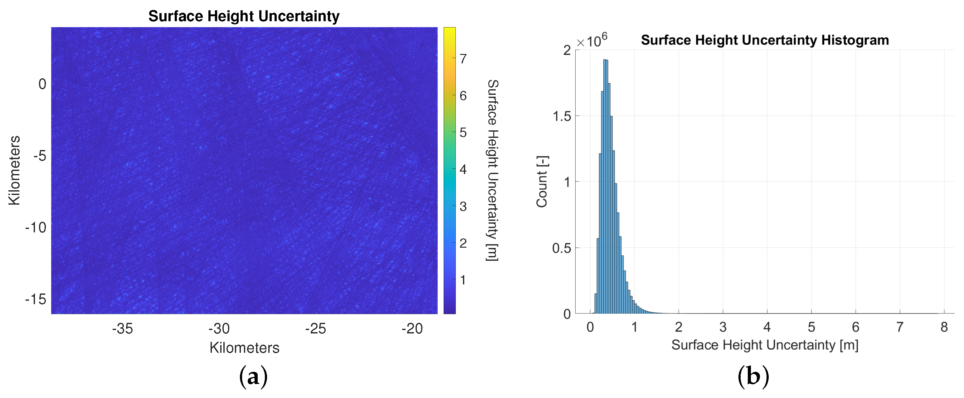
Figure 6a shows the surface height uncertainty related to the data component (accounting for the reduced orbital errors and interpolation errors). Note that the orbital tracks can be clearly observed, as for these pixels, the uncertainty is low (i.e., low interpolation error). The bright areas in Figure 6a represent areas for which the interpolation error is large. Figure 6b shows the histogram representing the altitude error due to orbital and interpolation errors. Most of the pixels have an error between 0 and 1 m.
The second term (geological component) is related to natural terrain variations and sub-pixel sampling (i.e., variation of the terrain within one pixel that cannot be captured in the DEM). This error is typically larger than the geolocation uncertainty [26]. To capture the magnitude of this error, detailed sub-pixel information is required (i.e., to detect the presence of rocks and boulders). As this information is not available, the 3-sigma covariance is used in the variance covariance analysis for the DEM measurement (note that the 1-sigma is shown in Equation (17)), accounting implicitly for this uncertainty.
The third term is related to the uncertainty of the rover receiver. In an ideal scenario, the receiver uncertainty would be zero, such that the right DEM pixel (and the associated height) could be selected and only data and geological errors remain. However, in a realistic scenario, the uncertainty of the receiver is non-zero, and as such, the selected pixel (based on the current receiver position) may not be correct. Depending on the variation of the terrain and the receiver uncertainty, this error may attain significant values (e.g., at the edge of a cliff).
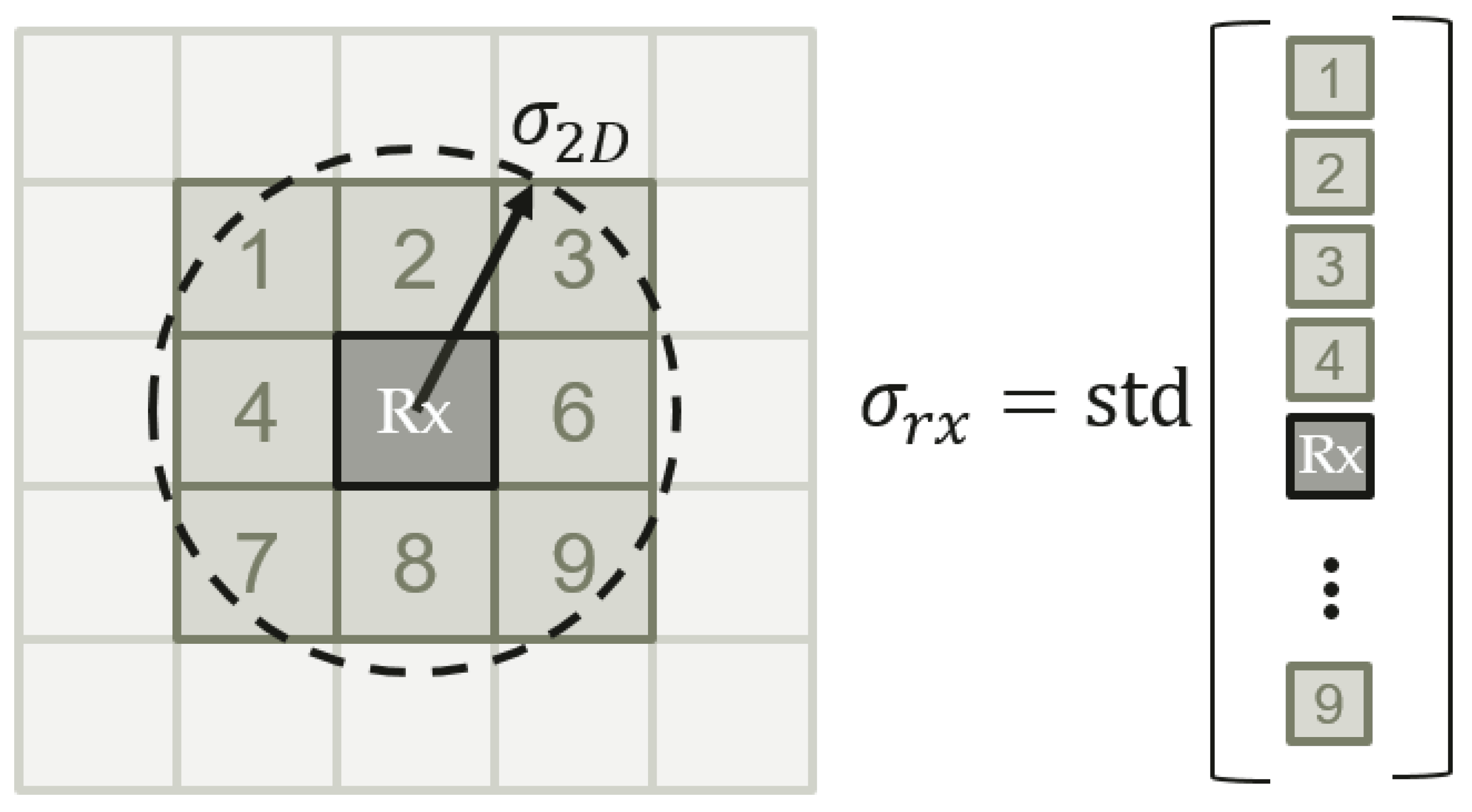
Figure 7 shows conceptually how the uncertainty of the rover is used to evaluate the associated uncertainty in the DEM measurement. It is assumed that the rover location (after the EKF propagation step) is somewhere in the pixel denoted with Rx. However, depending on the receiver horizontal covariance (denoted by ), the receiver may actually be located in another pixel with a different height. For example, assuming a horizontal receiver uncertainty of = 9 m and a DEM resolution of 5 m per pixel, the rover can be in any of the pixels indicated by 1–9. Subsequently, the standard deviation of all these pixels is used to evaluate the rover’s contribution to the uncertainty of the DEM measurement. Note that only the pixels for which the distance between the center of that pixel and the center of the pixel denoted with Rx is less than are used to evaluate . It is assumed that this approach will give a first-order estimate on the accuracy of the DEM measurement. A more complicated approach (e.g., considering the position history to select more probable pixels) can be considered for future work. However, in case the rover uncertainty is below 5 m (equal to the resolution of the DEM), at least the surrounding pixels (see Figure 7, pixels indicated 1–9) are used to compute the standard deviation, as the rover may be located in any of these pixels.
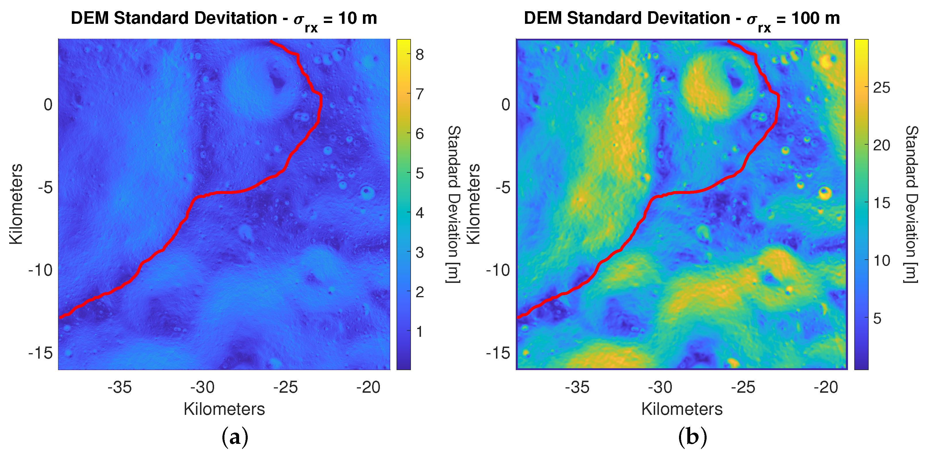
Figure 8a,b shows the standard deviation of the terrain surrounding each pixel considering a rover uncertainty (1) of, respectively, 10 m and 100 m. Figure 8a shows that a rover uncertainty of 10 m leads to a surrounding terrain standard deviation not larger than 8 m and actually much lower along the actual traverse. A 100 m receiver uncertainty leads to a surrounding terrain standard deviation up to 25–30 m (Figure 8b). The actual traverse shows lower values (below 15 m), confirming the good selection of the traverse (e.g., far from steep cliffs).
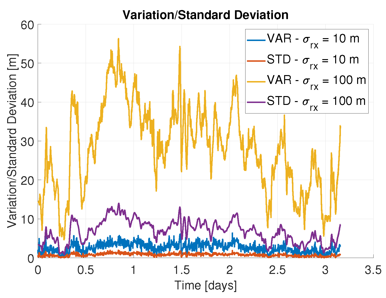
Figure 9 shows the variation of the terrain along the rover traverse introduced in Section 2 in terms of the standard deviation of all pixels within the circle covered by the horizontal uncertainty of the rover as well as the absolute variation between the minimum and maximum height experienced within the selected pixels. Note that both the standard deviation and absolute deviation considering a receiver uncertainty of 10 m are fairly low (below 5 m in most of the epochs). However, increasing the rover standard deviation to 100 m, the absolute variation attains significant values (e.g., above 50 m); nevertheless, the standard deviation remains low.
The overall DEM uncertainty is modelled by Equation (17), which contains the terms and , which, respectively, represent the uncertainty related to the data component (i.e., interpolation and orbital errors) as well as the DEM uncertainty induced by the rover horizontal uncertainty (which is defined as the standard deviation of all the pixels that are captured within a circle surrounding the propagated rover position consistent with Figure 7). and are assumed to be uncorrelated.
Finally, Table 8 shows the the parameters used in the DEM scenario. A threshold is used to disable the DEM aiding in case the current position uncertainty is too large. In such a case, the uncertainty of the receiver would lead to meaningless results. Furthermore, the n denotes the multiple of (i.e., 3-sigma for ) used in the measurement covariance matrix to account for the geological error component.
5. Results
5.1. Baseline
As indicated in Section 4.3, the positioning algorithms used for both the baseline solution (LCNS only) and the solution considering the DEM are similar (i.e., the same measurement model and process noise are used). The only difference occurs when the number of satellites is less than 4, in which case the range-rate observations are no longer used (as these require an accurate estimation of the clock drift).
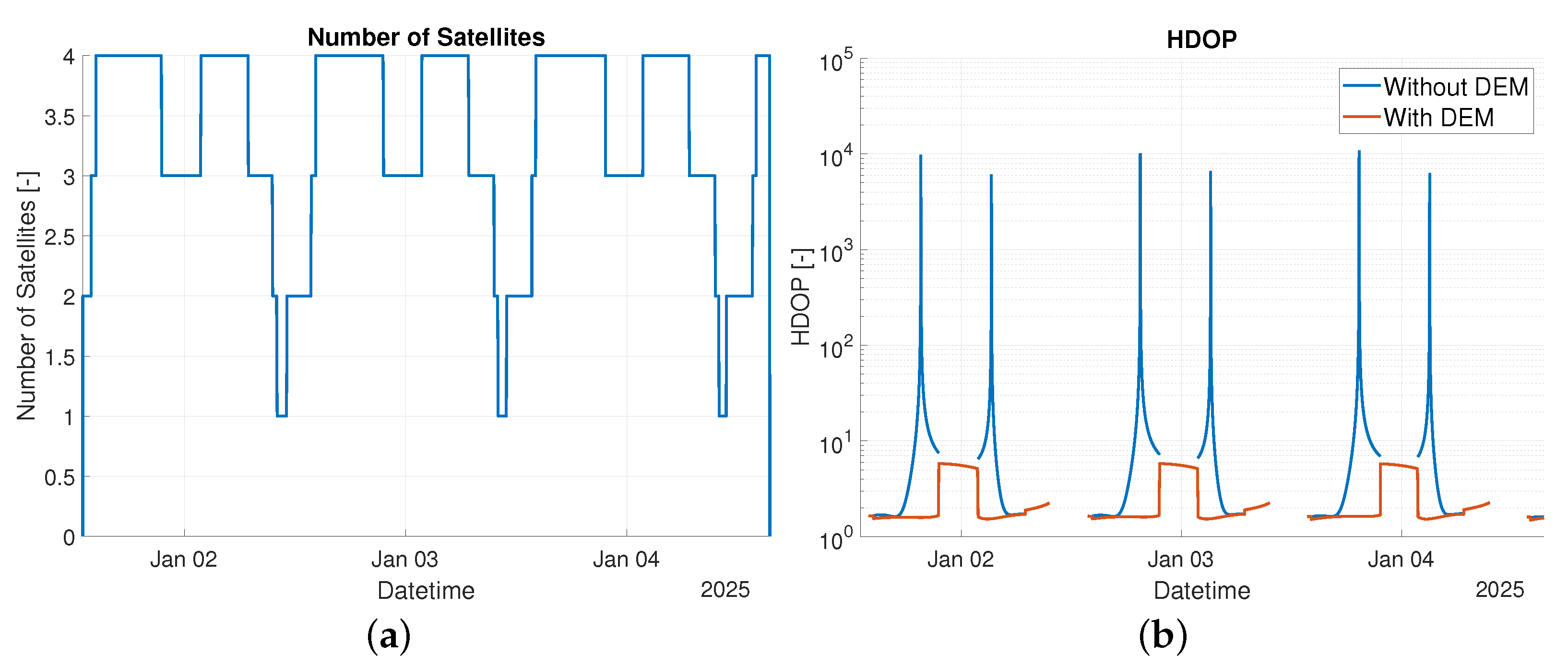
This section shows the results of the covariance analysis using the simulation parameters defined in Section 4.4. Figure 10a shows the number of visible satellites during the full scenario of approximately 3.1 days, while Figure 10b shows the horizontal dilution of precision (HDOP) of the solution with (red line) and without (blue line) the utilisation of DEM together with the LCNS measurements.
It can be clearly seen that the LCNS constellation introduced in Table 1 is optimized to ensure good coverage in the South pole, as 52% of the time, at least 4 satellites are visible. When comparing the HDOP of the solution with and without DEM, the added value of the DEM measurement is evident. While the HDOP of the satellite-only solution (without DEM) has peaks that reach values up to 10, the HDOP when using an additional DEM measurement is always below 10. Furthermore, the availability can be extended to the periods in which only 3 satellites are available, as the 3 satellite measurements and the additional DEM measurement allow the receiver to solve its three-dimensional position and clock bias. When less than 3 satellites are available, no solution is computed, so no HDOP is provided.
It is important to note that, within this contribution, it is assumed that the rover will continue moving even when no LCNS-based solution is available. This is possible using just IMU-based propagation or a visual-based odometer. When more than 3 satellites are again visible, the LCNS-based solution is re-started, considering the initial uncertainties in Table 6.
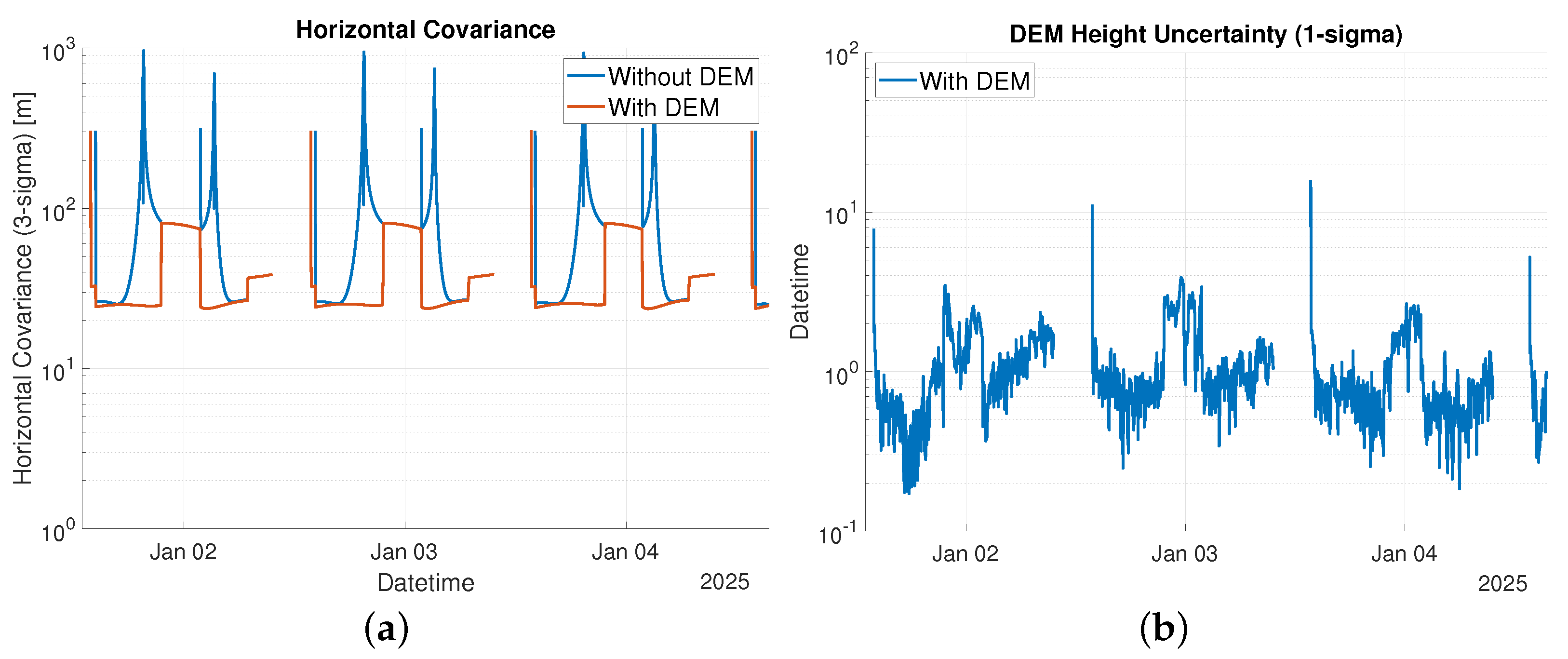
Figure 11a shows the horizontal (2D) covariance with (red line) and without (blue) the utilisation of the DEM. The behaviour of the horizontal covariance closely follows the behaviour of the HDOP, as reported in Figure 10b. The peaks at the beginning of each tracking period starting at 300 m (note that Figure 11a reports 3-sigma) indicate the convergence time needed as the filter is initialized at a position uncertainty of 100 m (as reported in Table 6). During the periods of good HDOP (satellite only), the performances between the satellite only and satellite and DEM solution are very similar; however, in case the geometry of the solution with the satellites degrades, having the DEM in the solution avoids a degradation of the solution accuracy. Furthermore, when only 3 satellites are visible, the LCNS-only solution cannot be computed, while with the additional DEM measurement, the rover is able to determine its position with reasonable performance (around 75 m 3-sigma).
Figure 11b shows the uncertainty (1-sigma) of the DEM measurement. The peaks (around 10 m) are caused by the initial rover uncertainty, which is set to 100 m (refer to Table 6) at the beginning of each tracking period. Once the receiver covariance has converged, it can be seen that the DEM uncertainty is primarily governed by the data component (refer to Section 4.5.2 for the definition of the data component), which is distributed between 0 and 1 m (refer to Figure 8b). Nevertheless, in the periods in which only three satellites are available, the rover uncertainty attains values above 10 m (related to the degraded HDOP) such that the rover-induced DEM covariance increases, as shown in Figure 11b.
Table 9 shows the statistics for the rover positioning with and without the usage of DEMs. It can be clearly seen that all statistics reported in Table 9 improve substantially when introducing the additional DEM observation into the positioning algorithm. The availability (e.g., percentage of the time the rover can determine its position) is increased from 52% to 82%, as the rover is able to determine its position with only 3 satellites when using the DEM. Furthermore, as also shown in Figure 11, the two periods in which 4 satellite are visible are now connected. As such, the period of continuous availability increases from slightly more than 5 h to almost 20 h. Note, as mentioned earlier, that the visibility window is expected to be better with the optimized orbital parameters under definition in the LCNS Phase A/B1 studies. Finally, the 68, 95 and 99.7 percentiles (considering the time variation of the 3-sigma horizontal covariance)of the horizontal position covariance are provided. As expected, the covariance is significantly reduced by constraining the vertical position with a very accurate measurement.
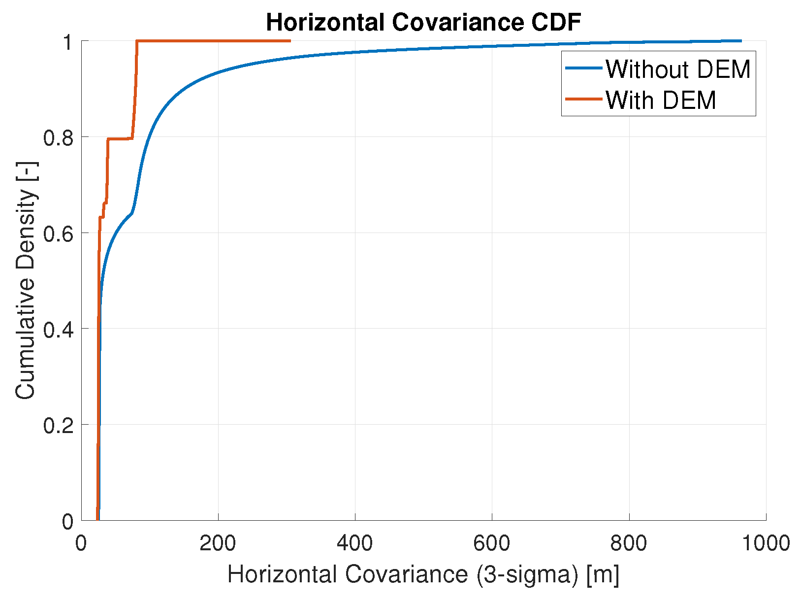
Figure 12 shows the cumulative density function (CDF) of the time variation of the horizontal covariance (3-sigma) for both the baseline (i.e., LCNS-only) and improved configuration (LCNS + DEM). While CDF is quite similar at lower uncertainties (until a CDF of 0.5), the CDF for the improved configuration (LCNS + DEM) is shifted to the left with respect to the baseline configuration (LCNS-only) mainly related to the improvement in geometry due to the additional DEM measurement.
5.2. Sensitivity Analysis ODTS
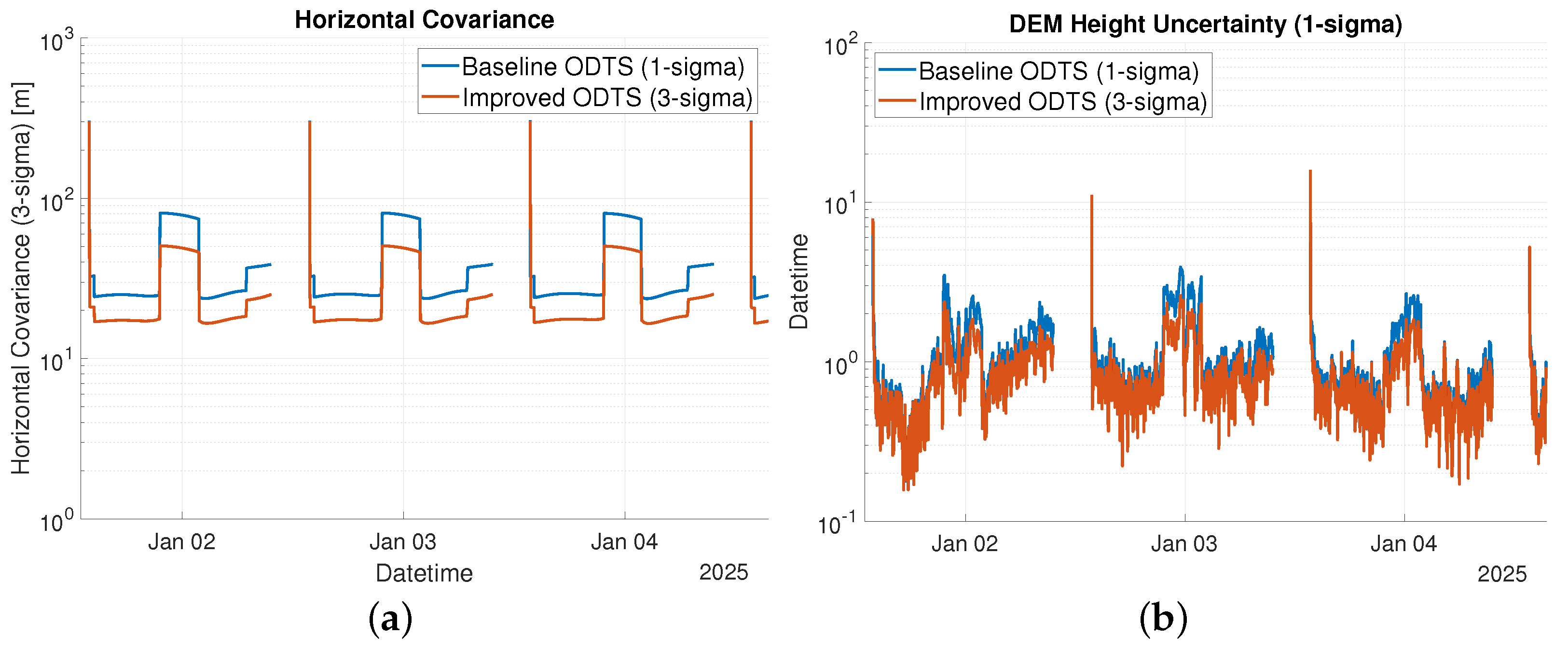
To understand the impact of the ODTS uncertainty on the attainable positioning, a sensitivity analysis was performed considering the values reported in Table 6 both as 1-sigma and 3-sigma. Figure 13a shows the horizontal covariance (3-sigma) of the lunar surface rover considering the baseline and improved ODTS uncertainties as indicated in Table 10. When using the improved scenario, the covariance is reduced by approximately 8 m (3-sigma) when the position has converged (in case of 4 visible satellites). For the slots in which 3 satellites are visible, this reduction is approximately 30 m (3-sigma).
An improvement in the ODTS accuracy affects the accuracy of the DEM measurement, as shown in Figure 13b. When only 3 satellites are visible, the horizontal covariance is smaller for the improved ODTS scenario. As such, the number of pixels considered to determine the variation of the terrain around the rover is smaller, which results in a smaller uncertainty of the DEM measurement.
5.3. Sensitivity Analysis Process Noise
As previously discussed in Section 4.2, the selection of the process noise matrix Q has a large impact on the attainable position accuracy. Therefore, this section shows the results of the sensitivity analysis for these critical parameters. Table 12 shows three different scenarios for the selection of process noise. The first scenario is in line with the definition of the process noise provided in Table 6, which assumes a relatively low quality IMU. Note that this level of process noise is in line with [29,32] assuming a tactical-grade IMU. However, the values used in the previous publications are considered conservative for a tactical-grade IMU. Therefore, in this paper, we aim to consider a more realistic process noise definition. The second and third scenario correspond to, respectively, a tactical- and navigation-grade IMU. Detailed characteristics of both types of IMU can be found in Table 4. The process noise for position and velocity is set to (note that these values are obtained from internal studies), characterizing the mismodeling of the kinematic filter. The process noise accounting for the IMU velocity random walk (defined in Table 4) is added to this value, leading to the values reported in Table 12, consistently with the definition of the process noise for a tightly coupled GNSS/INS filter [47].
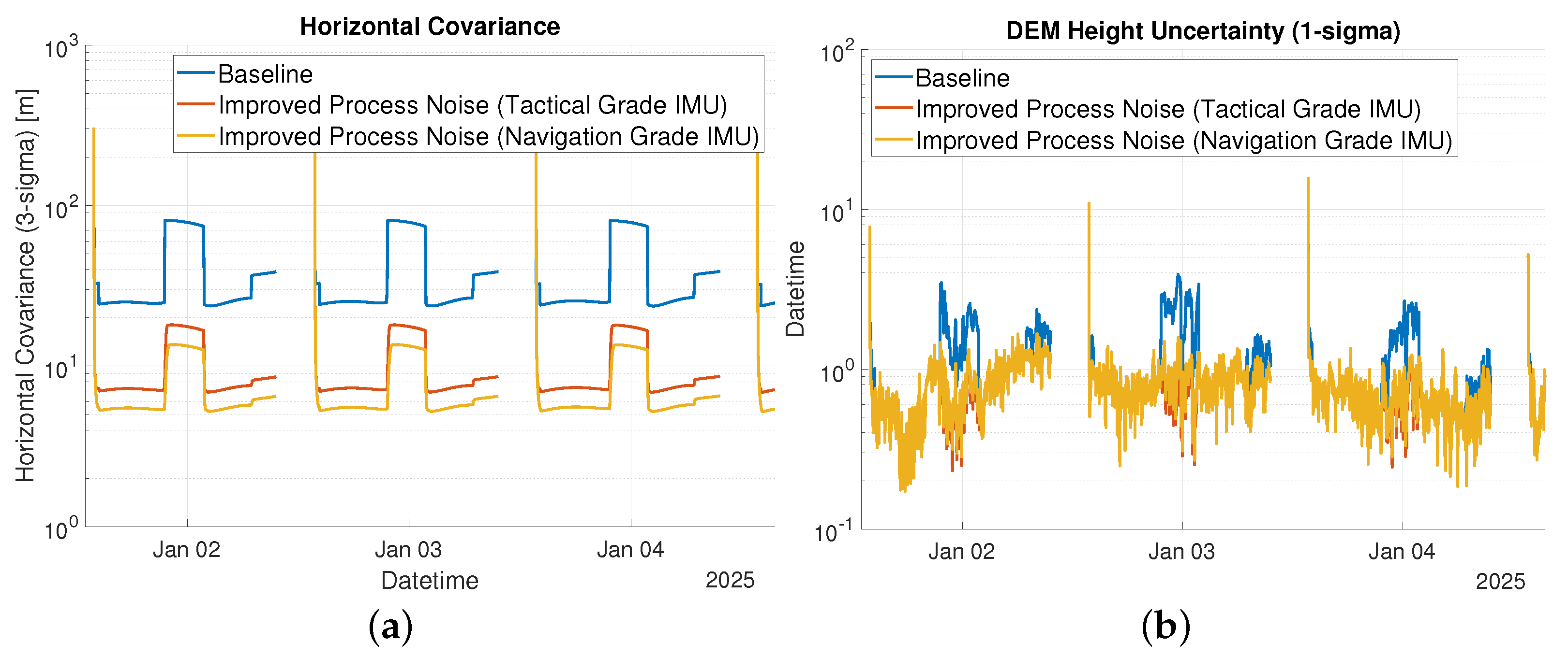
Figure 14a shows the horizontal covariance (3-sigma) for the three scenarios introduced in Table 12. It can be observed that the difference in attainable position accuracy between scenario 1 (baseline) and scenario 3 (navigation grade IMU) is almost an order of magnitude for the periods in which only 3 satellites are visible (Figure 10a). For the epochs in which 4 satellites are visible, the impact is less pronounced but still significant (approximately 20 m).
Figure 14b shows the uncertainty of the DEM measurement. Similar to the baseline scenario, the DEM uncertainty is primarily governed by the data component in case 4 satellites are available (as the horizontal uncertainty is within 5 m). However, contrary to the baseline scenario, scenarios 2 and 3 (tactical- and navigation-grade IMU) do not show the increase in the DEM uncertainty measurement during the periods in which only 3 satellites are visible, as its horizontal uncertainty is always below 2 m 1-sigma (except when initializing the EKF).
5.4. Sensitivity Analysis ODTS and Process Noise
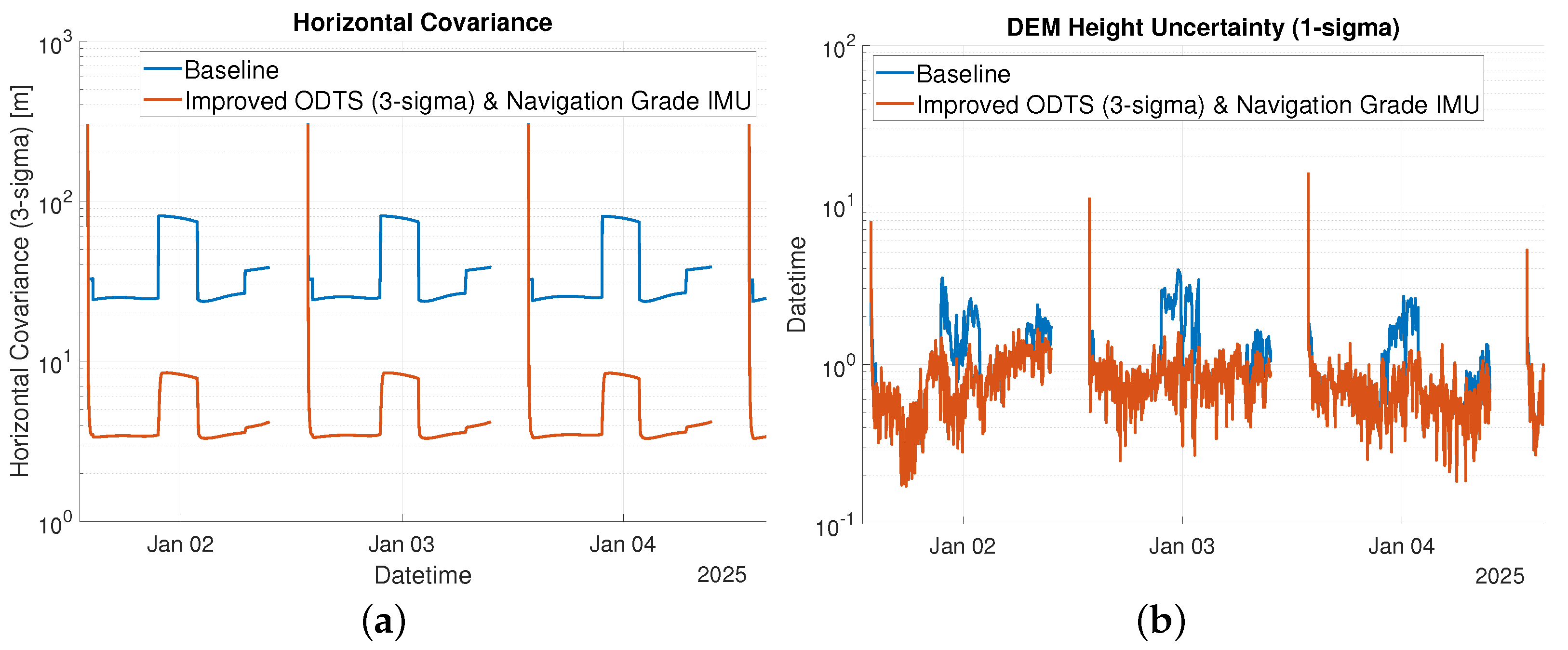
To understand what will be the ultimate achievable accuracy when considering the improved ODTS accuracy (i.e., 15 m position uncertainty 3-sigma) and a navigation-grade IMU (i.e., low process noise), both elements are combined in a single configuration. Figure 15a shows the horizontal covariance (3-sigma) for both the baseline scenario and the scenario considering the improved ODTS and navigation-grade IMU. It can be seen that the horizontal covariance (3-sigma) improves by almost one order of magnitude. Furthermore, note that the 3-sigma horizontal covariance is below 10 m for the complete duration of the traverse (except when the EKF is initialized). Figure 15b shows the DEM height uncertainty. As the horizontal covariance for the improved scenario is below 10 m, the uncertainty of the DEM measurement is almost uniquely defined by a data component.
6. Conclusions
The global space exploration roadmap assessed the gaps of robotic teleoperation in a report called “Telerobotic control of systems with time delay–Gap assessment report” [48]. One of the challenges identified is the location accuracy. In the report, the authors refer to Earth-based GNSS as one of the options to overcome this gap but indicate that such a service is not available in the lunar environment. The proposed LCNS system aims to cover this gap, providing accurate ranging signals than can be exploited, in real time, targeting both teleoperated or autonomous rovers as discussed this publication.
In this paper, we have shown that by constraining the height of the rover, using highly accurate digital elevation models that are available for the lunar South Pole, both the availability and accuracy of a lunar surface rover can be substantially improved. Furthermore, the proposed navigation solution operates under all illumination conditions and allows for a very repeatable and autonomous traverse: after the first traverse is performed, all subsequent traverses can be done fairly autonomously following the same path (as a path free of obstacles is found).
Using the available DEMs, the rover is able to continue to estimate its position while only 3 satellites are in view (contrary to the 4 satellites that are required without such a height constraint). This increases the availability of the navigation solution from 52% to 82%. Furthermore, by substantially reducing the HDOP by providing an additional measurement in the vertical direction (i.e., a direction which is typically poorly constrained for a satellite-based navigation system), the 3-sigma horizontal covariance is reduced from more than 800 m (considering the 99.7th percentile of the 3-sigma horizontal covariance) to less than 100 m, with very conservative assumptions for the IMU grade and the ODTS uncertainty.
A sensitivity analysis showed that an improvement of the LCNS ODTS accuracy does not have a major impact on the final performances (i.e., an improvement of the 3-sigma horizontal covariance by 8 m reducing the ODTS error by a factor of 3). An improvement of the IMU equipment, however, has a significant impact on the attainable performances, in particular when less than 4 satellites are tracked by the rover. This is expected as the IMU governs the process noise and the capability of the EKF to tighten the predictions and thus the final performances.
Considering both the improved ODTS accuracy and a navigation-grade IMU, the 99.7th percentile of the 3-sigma horizontal covariance can be reduced below 10 m (i.e., 8.6 m), allowing compliance with very stringent user requirements for surface-moving rovers (e.g., the NASA Lunar Communication Relay and Navigation services requirement LCRNS.3.0570, [49]). Note that the accuracy provided in this publication (3-sigma horizontal covariance) provides a first-order estimation on the type of accuracy that can be expected for a lunar rover using LCNS and DEMs to determine its position.
Considering the navigation-grade IMU, the final user position is mostly limited by the uncertainty on the DEM data component. This is intrinsic to the DEM data, and in principle, LCNS cannot provide a direct support to reduce it. However, LCNS can support future LOLA-like instruments, providing precise ranging data to improve the precise orbit determination of the satellites hosting the altimeter instrument and iteratively improve the DEM accuracy.
Even if variance-covariance analysis has some limitations (e.g., biases are not modelled), the use of 3-sigma in all error contributions allows to overbound stochastically the user accuracy capable of including a certain margin of biases coupled with the corresponding 1-sigma standard deviation.
This publication has shown that a simple 4-satellite constellation in lunar orbit and a user LCNS receiver that account for DEM and IMU measurements allow to achieve performances below 10 m 99.7 percent of the time over the traverse considered in this publication. Such performances meet the very stringent requirements expressed by space agencies and commercial users, allowing for larger autonomy and more safety in future lunar rovers.
7. Disclaimer
This publication does not cover the final Moonlight constellation, signals and service but rather presents what could be achieved with a lunar navigation satellite system. The actual Moonlight constellation, signals and related services will be defined as part of ESA programmes outside this publication.
Author Contributions
Conceptualization, F.T.M., P.Z., C.O., P.G. and J.V.-T.; methodology, F.T.M., P.Z., P.G. and R.S.; software and validation, F.T.M. and P.Z.; formal analysis, F.T.M.; investigation, F.T.M. and P.Z.; data curation, F.T.M.; writing—original draft preparation, F.T.M., P.Z. and P.G.; writing—review and editing, F.T.M., C.O., R.S. and J.V.-T.; visualization, F.T.M.; supervision, P.G. and J.V.-T. All authors have read and agreed to the published version of the manuscript.
Funding
This research received no external funding.
Acknowledgments
The authors would like to thank the anonymous reviewers for the valuable comments received.
Conflicts of Interest
The authors declare no conflict of interest.
Abbreviations
The following abbreviations are used in this manuscript:
| AOD | Age of Data |
| BPSK | Binary Phase Shift Keying |
| CDF | Cumulative Density Function |
| CNSA | China National Space Administration |
| DEM | Digital Elevation Model |
| DLL | Delay Locked Loop |
| DOP | Dilution of Precision |
| DSN | Deep Space Network |
| EIRP | Effective Isotropic Radiated Power |
| EKF | Extended Kalman Filter |
| ELFO | Elliptical Lunar Frozen Orbit |
| ESA | European Space Agency |
| FLL | Frequency Locked Loop |
| GIS | Geographic Information System |
| GNSS | Global Navigation Satellite System |
| GPS | Global Positioning System |
| HDOP | Horizontal Dilution of Precision |
| IMU | Inertial Measurement Unit |
| INS | Inertial Navigation System |
| JAXA | Japan Aerospace Exploration Agency |
| LANS | Lunar Augmented Navigation Service |
| LCNS | Lunar Communication and Navigation Services |
| LiASON | Linked Autonomous Interplanetary Satellite Orbit Navigation |
| LIDAR | LIght Detection and Ranging |
| LNA | Low Noise Amplifier |
| LOLA | Lunar Orbiter Laser Altimeter |
| LRO | Lunar Reconnaissance Orbiter |
| MER | Mars Exploration Rovers |
| NASA | National Aeronautics and Space Administration |
| OCXO | Oven Controlled Crystal Oscillator |
| ODTS | Orbit Determination and Time Synchronization |
| PDS | Planetary Data System |
| PLL | Phase Locked Loop |
| PNT | Position Navigation and Timing |
| RAAN | Right Ascension of the Ascending Node |
| RF | Radio Frequency |
| RFFE | Radio Frequency Front-End |
| SDD | Service Definition Document |
| SFCG | Space Frequency Coordination Group |
| SISE | Signal-in-Space Error |
| SPR | Small Pressurized Rover |
| VO | Visual Odometry |
References
- International Space Exploration Coordination Group. The Global Exploration Roadmap. 2018. Available online: https://www.nasa.gov/sites/default/files/atoms/files/ger_2018_small_mobile.pdf (accessed on 13 June 2022).
- Johnson, A.E.; Montgomery, J.F. Overview of terrain relative navigation approaches for precise lunar landing. In Proceedings of the IEEE Aerospace Conference, Big Sky, MT, USA, 1–8 March 2008; pp. 1–10. [Google Scholar]
- European Space Agency. Moonlight: Connecting Earth with the Moon. 2020. Available online: https://www.esa.int/ESA_Multimedia/Videos/2020/11/Moonlight_connecting_Earth_with_the_Moon/%28lang%29 (accessed on 23 June 2022).
- Lockheed Martin. Communicating with the Moon Is Getting Easier. 2022. Available online: https://www.lockheedmartin.com/en-us/news/features/2021/lunar-communication-and-navigation-network.html (accessed on 21 June 2022).
- GPS World. Ark Edge Space to Study Lunar Positioning, Communications for JAXA 2022. Available online: https://www.gpsworld.com/ark-edge-space-to-study-lunar-positioning-communications-for-jaxa/ (accessed on 21 June 2022).
- GPS World. Russia Plans to Place Positioning Satellites around the Moon 2018. Available online: https://www.gpsworld.com/russia-plans-to-place-positioning-satellites-around-the-moon/ (accessed on 21 June 2022).
- China.org.cn. China Starts Enginereing Development of Lunar Exploration Program’s Fourth Phase. 2022. Available online: http://www.china.org.cn/china/2022-04/25/content_78185065.htm (accessed on 21 June 2022).
- Draft LunaNet Interoperability Specifications. Technical report, NASA. 2022. Available online: https://esc.gsfc.nasa.gov/static-files/Draft%20LunaNet%20Interoperability%20Specification%20Final.pdf (accessed on 21 June 2022).
- Trexler, T.T.; Odden, R.B. Lunar Surface Navigation. IEEE Trans. Aerosp. Electron. Syst. 1966, AES-2, 252–259. [Google Scholar] [CrossRef]
- Yenilmez, L.; Temeltas, H. Autonomous navigation for planetary exploration by a mobile robot. In Proceedings of the International Conference on Recent Advances in Space Technologies, 2003. RAST’03, Istanbul, Turkey, 20–22 November 2003; pp. 397–402. [Google Scholar]
- Li, R.; Squyres, S.W.; Arvidson, R.E.; Archinal, B.A.; Bell, J.; Cheng, Y.; Crumpler, L.; Des Marais, D.J.; Di, K.; Ely, T.A.; et al. Initial results of rover localization and topographic mapping for the 2003 Mars Exploration Rover mission. Photogramm. Eng. Remote Sens. 2005, 71, 1129–1142. [Google Scholar] [CrossRef]
- Li, R.; Di, K.; Howard, A.B.; Matthies, L.; Wang, J.; Agarwal, S. Rock modeling and matching for autonomous long-range Mars rover localization. J. Field Robot. 2007, 24, 187–203. [Google Scholar] [CrossRef]
- Maimone, M.; Johnson, A.; Cheng, Y.; Willson, R.; Matthies, L. Autonomous navigation results from the Mars Exploration Rover (MER) mission. In Experimental Robotics IX; Springer: Berlin/Heidelberg, Germany, 2006; pp. 3–13. [Google Scholar]
- Goldberg, S.B.; Maimone, M.W.; Matthies, L. Stereo vision and rover navigation software for planetary exploration. In Proceedings of the IEEE Aerospace Conference, Big Sky, MT, USA, 9–16 March 2002; Volume 5, p. 5. [Google Scholar]
- Geromichalos, D.; Azkarate, M.; Tsardoulias, E.; Gerdes, L.; Petrou, L.; Perez Del Pulgar, C. SLAM for autonomous planetary rovers with global localization. J. Field Robot. 2020, 37, 830–847. [Google Scholar] [CrossRef]
- Carle, P.J.; Barfoot, T.D. Global rover localization by matching lidar and orbital 3d maps. In Proceedings of the IEEE International Conference on Robotics and Automation, Anchorage, AK, USA, 3–7 May 20; pp. 881–886.
- Matthies, L.; Daftry, S.; Tepsuporn, S.; Cheng, Y.; Atha, D.; Swan, R.M.; Ravichandar, S.; Ono, M. Lunar Rover Localization Using Craters as Landmarks. arXiv 2022, arXiv:2203.10073. [Google Scholar]
- Jun, W.W.; Cheung, K.M.; Lightsey, E.G.; Lee, C. A minimal architecture for real-time lunar surface positioning using joint Doppler and ranging. IEEE Trans. Aerosp. Electron. Syst. 2021, 58, 1367–1376. [Google Scholar] [CrossRef]
- Parker, T.; Golombek, M.; Powell, M. Geomorphic/geologic mapping, localization, and traverse planning at the Opportunity landing site, Mars. In Proceedings of the 4st Annual Lunar and Planetary Science Conference, The Woodlands, TX, USA, 1–5 March 2010; p. 2638, No. 1533. [Google Scholar]
- Chelmins, D.T.; Welch, B.W.; Sands, O.S.; Nguyen, B.V. A Kalman Approach to Lunar Surface Navigation Using Radiometric and Inertial Measurements; Technical Report; NASA: Washington, DC, USA, 2009. [Google Scholar]
- Hesar, S.G.; Parker, J.S.; Leonard, J.M.; McGranaghan, R.M.; Born, G.H. Lunar far side surface navigation using linked autonomous interplanetary satellite orbit navigation (LiAISON). Acta Astronaut. 2015, 117, 116–129. [Google Scholar] [CrossRef]
- Allender, E.J.; Orgel, C.; Almeida, N.V.; Cook, J.; Ende, J.J.; Kamps, O.; Mazrouei, S.; Slezak, T.J.; Soini, A.J.; Kring, D.A. Traverses for the ISECG-GER design reference mission for humans on the lunar surface. Adv. Space Res. 2019, 63, 692–727. [Google Scholar] [CrossRef]
- Li, S.; Lucey, P.G.; Milliken, R.E.; Hayne, P.O.; Fisher, E.; Williams, J.P.; Hurley, D.M.; Elphic, R.C. Direct evidence of surface exposed water ice in the lunar polar regions. Proc. Natl. Acad. Sci. USA 2018, 115, 8907–8912. [Google Scholar] [CrossRef] [PubMed]
- Smith, D.E.; Zuber, M.T.; Jackson, G.B.; Cavanaugh, J.F.; Neumann, G.A.; Riris, H.; Sun, X.; Zellar, R.S.; Coltharp, C.; Connelly, J.; et al. The lunar orbiter laser altimeter investigation on the lunar reconnaissance orbiter mission. Space Sci. Rev. 2010, 150, 209–241. [Google Scholar] [CrossRef]
- Tooley, C.R.; Houghton, M.B.; Saylor, R.S.; Peddie, C.; Everett, D.F.; Baker, C.L.; Safdie, K.N. Lunar Reconnaissance Orbiter mission and spacecraft design. Space Sci. Rev. 2010, 150, 23–62. [Google Scholar] [CrossRef]
- Barker, M.K.; Mazarico, E.; Neumann, G.A.; Smith, D.E.; Zuber, M.T.; Head, J.W. Improved LOLA elevation maps for south pole landing sites: Error estimates and their impact on illumination conditions. Planet. Space Sci. 2021, 203, 105119. [Google Scholar] [CrossRef]
- Barker, M.; Mazarico, E.; Neumann, G.; Zuber, M.; Haruyama, J.; Smith, D. A new lunar digital elevation model from the Lunar Orbiter Laser Altimeter and SELENE Terrain Camera. Icarus 2016, 273, 346–355. Available online: http://imbrium.mit.edu/ (accessed on 9 August 2022). [CrossRef]
- Delépaut, A.; Giordano, P.; Ventura-Traveset, J.; Blonski, D.; Schönfeldt, M.; Schoonejans, P.; Aziz, S.; Walker, R. Use of GNSS for lunar missions and plans for lunar in-orbit development. Adv. Space Res. 2020, 66, 2739–2756. [Google Scholar] [CrossRef]
- Grenier, A.; Giordano, P.; Bucci, L.; Cropp, A.; Zoccarato, P.; Swinden, R.; Ventura-Traveset, J. Positioning and Velocity Performance Levels for a Lunar Lander using a Dedicated Lunar Communication and Navigation System. Navig. J. Inst. Navig. 2022, 69, navi.513. [Google Scholar] [CrossRef]
- Barton, G.H.; Sheppard, S.W.; Brand, T.J. Proposed autonomous lunar navigation system. Astrodynamics 1993, 1993, 1717–1736. [Google Scholar]
- Schönfeldt, M.; Grenier, A.; Delépaut, A.; Giordano, P.; Swinden, R.; Ventura-Traveset, J. Across the Lunar Landscape: Towards a Dedicated Lunar PNT System. Inside GNSS. 2020. Available online: https://insidegnss.com/across-the-lunar-landscape-exploration-with-gnss-technology/ (accessed on 9 August 2022).
- Giordano, P.; Grenier, A.; Zoccarato, P.; Bucci, L.; Cropp, A.; Swinden, R.; Gomez Otero, D.; El-Dali, W.; Carey, W.; Duvet, L.; et al. Moonlight navigation service-how to land on peaks of eternal light. In Proceedings of the 72nd International Astronautical Congress (IAC), Dubai, United Arab Emirates, 25–29 October 2021. [Google Scholar]
- Space Frequency Coordination Group. Communication AND Positioning, Navigation, and Timing Frequency Allocations and Sharing in the Lunar Region. 2021. Available online: https://www.sfcgonline.org/Recommendations/REC%20SFCG%2032-2R3%20(Freqs%20for%20Lunar%20region).pdf (accessed on 14 June 2022).
- Giordano, P.; Melman, F.; Swinden, R.; Zoccarato, P.; Ventura-Traveset, J. The Lunar Pathfinder PNT Experiment and Moonlight Navigation Service: The Future of Lunar Position, Navigation and Timing. In Proceedings of the 2022 International Technical Meeting of The Institute of Navigation, Long Beach, CA, USA, 23–26 January 2023; pp. 632–642. [Google Scholar]
- Analytical Graphics Inc. Using Communication Constraints to Design Communication Links. 2016. Available online: https://help.agi.com/stk/11.0.1/Content/training/Constraints.htm (accessed on 5 August 2022).
- Das, P.; Ortega, L.; Vilà-Valls, J.; Vincent, F.; Chaumette, E.; Davain, L. Performance limits of GNSS code-based precise positioning: GPS, galileo & meta-signals. Sensors 2020, 20, 2196. [Google Scholar]
- Northtrop Grumman. LN-200S: Inertial Measurement Unit (IMU). 2021. Available online: https://www.northropgrumman.com/wp-content/uploads/LN-200S-Inertial-Measurement-Unit-IMU-datasheet.pdf (accessed on 20 June 2022).
- iMAR. iNAV-RQH-1001. 2014. Available online: https://www.imar-navigation.de/downloads/NAV_RQH_1001_en.pdf (accessed on 21 June 2022).
- Vectron Oscillators. OX-249 Space Qualified Oven Controlled Crystal Osciallator (OCXO). 2021. Available online: https://www.vectron.com/products/ocxo/OX-249.pdf (accessed on 14 June 2022).
- AXTAL GmbH. AXIOM6060: Ultra-Low Phase Noise 100 MHz OCXO for Space Application. 2015. Available online: https://www.axtal.com/cms/docs/doc91629.pdf (accessed on 14 June 2022).
- AXTAL GmbH. AXIOM70SL: Ultra-Low Phase Noise 10 MHz OCXO with HCMOS Output for Space Application (Space COTS version). 2022. Available online: https://www.axtal.com/cms/docs/doc124949.pdf (accessed on 14 June 2022).
- Brown, R.; Whang, P. Introduction to Random Signals and Applied Kalman Filtering; John Wiley & Sons, Inc.: New York, NY, USA, 1992; Volume 152. [Google Scholar]
- Montenbruck, O.; Gill, E. Satellite Orbits; Springer: Berlin/Heidelberg, Germany, 2013. [Google Scholar]
- European Commission. European GNSS (Galileo) Open Service Definition Document. 2021. Available online: https://www.gsc-europa.eu/sites/default/files/sites/all/files/Galileo-OS-SDD_v1.2.pdf (accessed on 14 June 2022).
- Petovello, M.; Cannon, M.; Lachapelle, G. Benefits of using a tactical-grade IMU for high-accuracy positioning. Navigation 2004, 51, 1–12. [Google Scholar] [CrossRef]
- Kaplan, E.D.; Hegarty, C. Understanding GPS/GNSS: Principles and Applications; Artech House: Norwood, MA, USA, 2017. [Google Scholar]
- Farrell, J. Aided Navigation: GPS with High Rate Sensors; McGraw-Hill, Inc.: New York, NY, USA, 2008. [Google Scholar]
- International Space Exploration Coordination Group. Telerobotics Control of Systems with Time Delay–Gap Assessment Report. 2018. Available online: https://www.globalspaceexploration.org/wordpress/docs/Telerobotic%20Control%20of%20Systems%20with%20Time%20Delay%20Gap%20Assessment%20Report.pdf (accessed on 14 June 2022).
- Lunar Communications Relay and Navigation Systems (LCRNS)–Preliminary Lunar Relay Services Requirements Document (SRD). Technical Report, NASA. 2022. Available online: https://esc.gsfc.nasa.gov/static/2fbc056474937c4e3ecfdba1dc595f06/ee60f0dad022948b2e8ce03e6e86a2f0.pdf (accessed on 24 June 2022).
Figure 1.
Lunar South Pole traverse shown on top of a low resolution DEM (100 m/pixel) available at the LOLA Planetary Data System (PDS) archive [27], while the small square indicates the region for which a high resolution DEM at 5 m/pixel is available. Projection is polar stereographic where (0, 0) denotes the South Pole.

Figure 2.
Rover altitude profile within the coverage of the high-resolution DEM. (a) shows the rover height above the Selenoid, while (b) shows the slope given by the DEM.
Figure 2.
Rover altitude profile within the coverage of the high-resolution DEM. (a) shows the rover height above the Selenoid, while (b) shows the slope given by the DEM.

Figure 3.
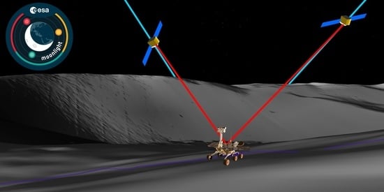
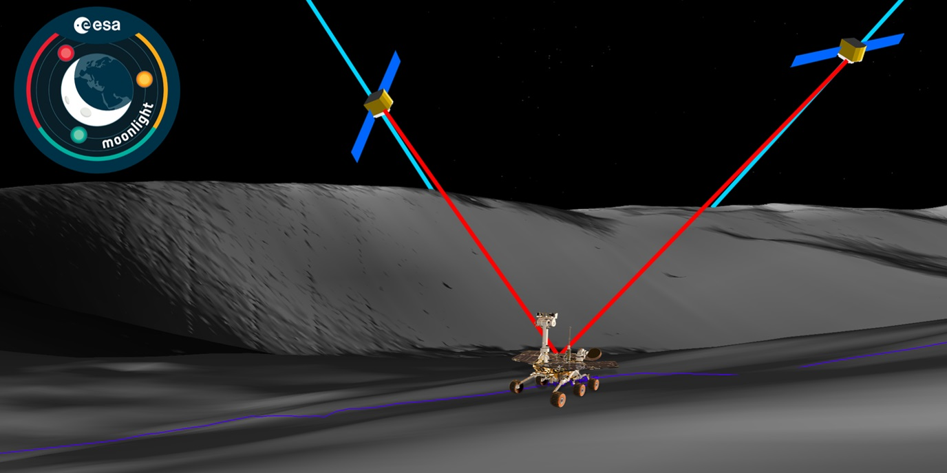
(a) Part of the lunar traverse shown in Figure 1 considered in this paper. The terrain topography shown is simulated using the high-resolution DEM provided (5 m/pixel) in the LOLA PDS archive [27]. The left part of the traverse follows the southern rim of the de Gerlache crater, while the right part descends into the direction of the Shackleton crater. (b) shows the Moonlight Logo.
Figure 3.
(a) Part of the lunar traverse shown in Figure 1 considered in this paper. The terrain topography shown is simulated using the high-resolution DEM provided (5 m/pixel) in the LOLA PDS archive [27]. The left part of the traverse follows the southern rim of the de Gerlache crater, while the right part descends into the direction of the Shackleton crater. (b) shows the Moonlight Logo.

Figure 4.
Antenna pattern of the LCNS satellites.

Figure 5.
Antenna pattern of the receiver.

Figure 6.
Surface Height Uncertainty (). (a) shows the surface height uncertainty (data from [26]) related to the data component for each pixel of the DEM (the projection is polar stereographic, where (0,0) denotes the South Pole), while (b) shows the histogram for all pixels shown in (a). Note that the scale of the x and y axes of (a) is not equal.

Figure 7.
Conceptual drawing showing how the uncertainty related to the DEM measurement is evaluated based on the rover’s horizontal uncertainty.
Figure 7.
Conceptual drawing showing how the uncertainty related to the DEM measurement is evaluated based on the rover’s horizontal uncertainty.

Figure 8.
Standard deviation () of the lunar terrain surrounding the rover traverse (in red). (a) shows the standard deviation of the terrain height considering all pixels which have their centre within 10 m of the query point, while (b) shows the standard deviation for all pixels which have their centre within 100 m of the query point. The projection is polar stereographic, where (0, 0) denotes the South Pole.

Figure 9.
Variation in the terrain along the traverse of the rover considering both the standard deviation (STD) and the absolute deviation (VAR) and considering a rover horizontal uncertainty of both 10 m and 100 m.
Figure 9.
Variation in the terrain along the traverse of the rover considering both the standard deviation (STD) and the absolute deviation (VAR) and considering a rover horizontal uncertainty of both 10 m and 100 m.

Figure 10.
Geometry of the scenario. (a) shows the number of visible satellites in time, while (b) shows the HDOP considering both the LCNS-only and LCNS + DEM scenarios.
Figure 10.
Geometry of the scenario. (a) shows the number of visible satellites in time, while (b) shows the HDOP considering both the LCNS-only and LCNS + DEM scenarios.

Figure 11.
Performance of the LCNS position solution. (a) shows the horizontal (2D) covariance (3-sigma) of both the LCNS-only as well as the LCNS and DEM solution, while (b) shows the 1-sigma uncertainty of the DEM measurement.
Figure 11.
Performance of the LCNS position solution. (a) shows the horizontal (2D) covariance (3-sigma) of both the LCNS-only as well as the LCNS and DEM solution, while (b) shows the 1-sigma uncertainty of the DEM measurement.

Figure 12.
Cumulative density function of the 3-sigma horizontal covariance (considering the time domain).
Figure 12.
Cumulative density function of the 3-sigma horizontal covariance (considering the time domain).

Figure 13.
Performance of the LCNS position solution. (a) shows the horizontal (2D) covariance of both the LCNS-only as well as the LCNS and DEM solution, while (b) shows the 1-sigma uncertainty of the DEM measurement.
Figure 13.
Performance of the LCNS position solution. (a) shows the horizontal (2D) covariance of both the LCNS-only as well as the LCNS and DEM solution, while (b) shows the 1-sigma uncertainty of the DEM measurement.

Figure 14.
Performance of the LCNS position solution. (a) shows the horizontal (2D) covariance of for the different process noise scenarios identified in Table 12, while (b) shows the 1 uncertainty of the DEM measurement for the different process noise scenarios identified in Table 12.

Figure 15.
Performance of the LCNS position solution. (a) shows the horizontal (2D) covariance of for the baseline and improved scenarios (considering an improved ODTS accuracy and navigation-grade IMU, while (b) shows the 1-sigma uncertainty of the DEM measurement for the same scenarios as defined in (a).

Table 1.
Kepler elements of the LCNS ELFO orbits. Note that the orbits have not been optimised and are therefore not representative of the Moonlight orbits. RAAN refers to the right ascension of the ascending node.
Table 1.
Kepler elements of the LCNS ELFO orbits. Note that the orbits have not been optimised and are therefore not representative of the Moonlight orbits. RAAN refers to the right ascension of the ascending node.
| Satellite Number | Semi-Major Axis | Eccentricity | Inclination | Argument of Pericenter | RAAN | True Anomaly |
|---|---|---|---|---|---|---|
| 1 | 9750.73 km | 0.6383 | 54.33 | 55.18 | 277.53 | 123.42 |
| 2 | 9750.73 km | 0.6383 | 54.33 | 55.18 | 277.53 | 0 |
| 3 | 9750.73 km | 0.6383 | 61.96 | 121.7 | 59.27 | 180 |
| 4 | 9750.73 km | 0.6383 | 61.96 | 121.7 | 59.27 | 0 |
Table 2.
Characteristics of the proposed LCNS signal.
| Element | Parameter | Value |
|---|---|---|
| Signal Carrier | Carrier Frequency () | 2491.005 MHz |
| Carrier Wavelength () | 12.04 cm | |
| Signal Modulation | Chipping Frequency () | BPSK(5) |
| Chip Length () | 58.61 m |
Table 3.
Characteristics of the rover LCNS S-band receiver.
| Parameter | Value |
|---|---|
| RF Front-end Noise Figure | 1 dB |
| Noise Temperature | 113 K |
| LNA Gain | 30 dB |
| Coherent Integration Time () | 20 ms |
| cutoff | 30 dB-Hz |
Table 6.
Configuration settings used for the EKF covariance analysis; all values are 1-sigma.
| Parameter | State Vector Element | Value |
|---|---|---|
| LCNS ODTS Uncertainty (1-sigma) | Position () | 15 m |
| Velocity () | 0.15 m/s | |
| Clock () | 10 m | |
| Clock drift () | 0.1 m/s | |
| EKF Process Noise (1-sigma) | Position () | 0.01 m/ |
| Velocity () | 0.15 m/s/ | |
| Clock () | 1 m/ | |
| Clock drift () | 10 m/s/ | |
| Intitial EKF Uncertainty (1-sigma) | Position | 100 m |
| Velocity | 10 m/s | |
| Clock | 100 m | |
| Clock drift | 1 m/s |
Table 7.
Configuration settings used for the EKF covariance analysis.
| Parameter | Value |
|---|---|
| DLL Loop bandwidth () | 0.5 Hz |
| FLL Loop bandwidth () | 10 Hz |
| Coherent integration time () | 20 ms |
| Early-late spacing (d) | 1 chip |
Table 8.
DEM simulation parameters.
| Parameter | Value |
|---|---|
| Threshold to enable DEM measurement | 150 m |
| Multiplier n for | 3 |
Table 9.
Statistics highlighting the gain in performance when using a DEM. The percentiles refer to the time series of the horizontal uncertainty (3-sigma).
Table 9.
Statistics highlighting the gain in performance when using a DEM. The percentiles refer to the time series of the horizontal uncertainty (3-sigma).
| Scenario | Availability [%] | Longest Continuous Availability [hr] | 68th Percentile [m] | 95th Percentile [m] | 99.7th Percentile [m] |
|---|---|---|---|---|---|
| 1. Without DEM | 52.0 | 5.2 | 80.3 | 242.8 | 810.2 |
| 2. With DEM | 82.2 | 19.9 | 37.2 | 80.3 | 81.0 |
Table 10.
ODTS uncertainty definition per scenario type.
| Scenario | Position [m] | Velocity [m/s] | Clock Bias [m] | Clock Drift [m/s] |
|---|---|---|---|---|
| 1. Baseline (1-sigma 1) | 15 | 0.15 | 10 | 0.1 |
| 2. Improved (3-sigma 1) | 5 | 0.05 | 3.333 | 0.033 |
1 The ODTS uncertainty reported in Table 6 is the baseline for both scenarios. In the first scenario (i.e., baseline), these values are considered as 1-sigma and are used directly in the simulation. In the second scenario (i.e., improved), these values are considered 3-sigma and therefore divided by 3 before they are used in the simulation (note that the simulator always uses the 1-sigma values).
Table 11.
Statistics highlighting the improved position accuracy in case of an improved ODTS accuracy. The percentiles refer to the time series of the horizontal uncertainty (3-sigma).
Table 11.
Statistics highlighting the improved position accuracy in case of an improved ODTS accuracy. The percentiles refer to the time series of the horizontal uncertainty (3-sigma).
| Scenario | 68th Percentile [m] | 95th Percentile [m] | 99.7th Percentile [m] |
|---|---|---|---|
| 1. Baseline ODTS | 37.2 | 80.3 | 81.0 |
| 2. Improved ODTS | 23.4 | 50.1 | 50.6 |
Table 12.
Process noise definition per scenario type.
| Scenario | [m/] | [m/s/] | [m/] | [m/s/] |
|---|---|---|---|---|
| 1. Baseline | 0.01 | 0.15 | 1 | 10 |
| 2. Improved (Tactical-Grade IMU) | 1 | 10 | ||
| 3. Improved (Navigation-Grade IMU) | 1 | 10 |
Table 13.
Statistics highlighting the gain in performance when improving the EKF process noise (by changing the type of IMU). The percentiles refer to the time series of the horizontal uncertainty (3-sigma).
Table 13.
Statistics highlighting the gain in performance when improving the EKF process noise (by changing the type of IMU). The percentiles refer to the time series of the horizontal uncertainty (3-sigma).
| Scenario | 68th Percentile [m] | 95th Percentile [m] | 99.7th Percentile [m] |
|---|---|---|---|
| 1. Baseline | 37.2 | 80.3 | 81.0 |
| 2. Improved (Tactical-Grade IMU) | 8.3 | 17.9 | 18.1 |
| 3. Improved (Navigation-Grade IMU) | 6.3 | 13.5 | 15.3 |
Table 14.
Statistics highlighting the gain in performance in case of an improved ODTS accuracy and a navigation-grade IMU. The percentiles refer to the time series of the horizontal uncertainty (3-sigma).
Table 14.
Statistics highlighting the gain in performance in case of an improved ODTS accuracy and a navigation-grade IMU. The percentiles refer to the time series of the horizontal uncertainty (3-sigma).
| Scenario | 68th Percentile [m] | 95th Percentile [m] | 99.7th Percentile [m] |
|---|---|---|---|
| 1. Baseline | 37.2 | 80.3 | 81.0 |
| 2. Improved ODTS and Tactical-Grade IMU | 3.9 | 8.4 | 8.6 |
Publisher’s Note: MDPI stays neutral with regard to jurisdictional claims in published maps and institutional affiliations. |
© 2022 by the authors. Licensee MDPI, Basel, Switzerland. This article is an open access article distributed under the terms and conditions of the Creative Commons Attribution (CC BY) license (https://creativecommons.org/licenses/by/4.0/).
Share and Cite
MDPI and ACS Style
Melman, F.T.; Zoccarato, P.; Orgel, C.; Swinden, R.; Giordano, P.; Ventura-Traveset, J. LCNS Positioning of a Lunar Surface Rover Using a DEM-Based Altitude Constraint. Remote Sens. 2022, 14, 3942. https://doi.org/10.3390/rs14163942
AMA Style
Melman FT, Zoccarato P, Orgel C, Swinden R, Giordano P, Ventura-Traveset J. LCNS Positioning of a Lunar Surface Rover Using a DEM-Based Altitude Constraint. Remote Sensing. 2022; 14(16):3942. https://doi.org/10.3390/rs14163942
Chicago/Turabian StyleMelman, Floor Thomas, Paolo Zoccarato, Csilla Orgel, Richard Swinden, Pietro Giordano, and Javier Ventura-Traveset. 2022. "LCNS Positioning of a Lunar Surface Rover Using a DEM-Based Altitude Constraint" Remote Sensing 14, no. 16: 3942. https://doi.org/10.3390/rs14163942
Note that from the first issue of 2016, this journal uses article numbers instead of page numbers. See further details here.