
Monitoring Land Vegetation from Geostationary Satellite Advanced Himawari Imager (AHI)

1
School of Atmospheric Physics, Nanjing University of Information Science and Technology, Nanjing 210044, China
2
CMA Earth System Modeling and Prediction Centre, Beijing 100081, China
3
National Satellite Meteorological Center, Beijing 100081, China
*
Author to whom correspondence should be addressed.
Remote Sens. 2022, 14(15), 3817; https://doi.org/10.3390/rs14153817
Submission received: 23 June 2022
/
Revised: 1 August 2022
/
Accepted: 2 August 2022
/
Published: 8 August 2022
(This article belongs to the Special Issue Atmospheric and Surface Modeling, Data Assimilation, and Forecasting of Remote Sensing)
Abstract
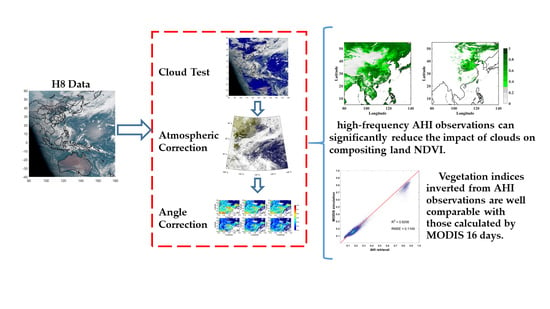
:For many years, the Advanced Very High-Resolution Radiometer (AVHRR) and Moderate Resolution Imaging Spectroradiometer (MODIS) instruments have been widely used to monitor the condition of surface vegetation. Since the polar-orbiting satellite provides limited daily samples on surface, a completed spatial coverage of land vegetation is often relied on over multiple days of observations. In this study, observations from the Japanese geostationary satellite imager Advanced Himawari Imagers (AHI) are used to derive the surface vegetation index. The AHI reflectance at visible and near-infrared bands are first corrected to the surface reflectance by using the 6S radiative transfer model. The AHI surface reflectance from various viewing angles and solar geometry is further normalized to form an angular-independent reflectance by using a BRDF model. Finally, the surface vegetation index is calculated and synthesized from the daytime AHI data. It is found that the high-frequency AHI observations can significantly reduce the impact of clouds on compositing land NDVI and require a shorter time for a complete coverage of surface conditions. Also, a single NDVI image from AHI exhibits spatial distribution similar to that from 16 days of MODIS data.
1. Introduction
Vegetation is the natural link between surface and atmosphere [1]. It plays an important role in global climate change and regional ecology. Surface vegetation is now being monitored with various techniques for real-time understanding of the earth’s ecological environment. The Normalized Difference Vegetation Index (NDVI) is one of the most commonly used indices in the field of remote sensing and is widely used in vegetation monitoring, disaster assessment, climate analysis, and land surface models [2,3]. NDVI measures the difference between near-infrared (strongly reflective) and red (vegetation-absorbing) reflectance to quantify the vegetation conditions, and is calculated as:
where and are the reflectance of NIR and red light, respectively. Equation (1) was introduced by Deering in 1978 and limits the ratio to the range (−1, 1) [4]. NDVI has also been widely applied to global and regional land cover, vegetation classification and environmental change, net primary vegetation productivity (NPP), crop and forage yield estimation, etc. [5]. In order to respond to a variety of application needs, NDVI products are now being generated with a high spatial resolution for monitoring of dynamic land cover change, emergency rescue, disaster monitoring, agricultural yield estimation and many other fields.
The satellite-derived NDVI is very much dependent on the instrument characteristics and the retrieval process as to whether the atmospheric and scan angle effects are corrected. The NDVI products from AVHRR are significantly higher than those from MODIS and seem to have a wider dynamic range [2]. The difference may be also related to the different spectral response functions of two instruments: the MODIS spectral response range is much narrower than AVHRR and also the effects of water vapor and aerosols on the reflectance have been removed in MODIS NDVI [6]. Comparing to MODIS NDVI, the products of Suomi NPP VIIRS are very similar in magnitudes since the spectral response functions and data processing processes for both sensors are similar [7,8,9].
A single polar-orbiting satellite only observes a region at a fixed local time. It generally only once a day and offers very limited NDVI information. Due to the presence of clouds, surface information for a specific area may only be observed from a period of satellite observations. For example, a 16-day synthesis period is proposed for MODIS NDVI, and the minimum 10-day synthesis period for AVHRR NDVI [10]. The change in NDVI within the period of synthesis is not well understood from the current polar NDVI products.
Polar-orbiting satellite measurements are often composited over a large area in order to get the NDVI information within a similar viewing geometry. However, the geometry of the sun–object–sensor relationship varies with each observation. This change may directly affect the quality of vegetation index. While the MODIS synthesis scheme is designed to take into account the variation of the satellite zenith angle, it remains difficult to compare the products from the two polar-orbiting satellites flying in different orbits (morning or afternoon). This is evidenced by the difference between the MODIS MOD products from the EOS Aqua satellite and MYD products from the EOS Terra satellite.
While the polar-orbiting satellite data have been extensively used for monitoring surface vegetation, the advantages of geostationary satellites are not well explored for NDVI calculation. The Advanced Himawari Imager carried onboard the Himawari-8 satellite has a spatial resolution of 1 km in visible bands and a temporal resolution of 10 min [11]. Multiple looks at the same area from geostationary satellites during a day can reduce the influence of clouds on the vegetation monitoring. Thus, the goal of this study was to use the AHI to derive the surface vegetation index.
This paper is organized as follows: In the next section, AHI instruments and data are described, and the retrieval algorithm for geostationary satellite application is then presented. In Section 3, the retrieved NDVI products composited from a single day are demonstrated. Finally, some discussions and conclusions are presented.
2. Data and Methodology
2.1. Advanced Himawari Imager (AHI) Data
Himawari-8 and Himawari-9 satellites have a payload called the Advanced Himawari Imager (AHI) for dedicated meteorological mission. Table 1 shows the AHI observation bands. The functions and specifications are notably improved from those of the imagers on board previous generation of MTSATs. Today, AHI has widely been used in now-casting. According to international community reports, it improved numerical weather prediction accuracy and enhanced environmental monitoring [12]. AHI scans a full disk of earth within 10 min at a spatial resolution of 0.5 km for blue and green bands and 1 km in red and near-IR bands [11]. Great RGB color images can be derived by compositing three visible bands (blue: 0.47 µm; green: 0.51 µm; red: 0.64 µm). However, the quantitative uses of these bands for surface vegetation monitoring is yet to be fully explored.
The spectral response functions (SRF) are very important for surface vegetation studies. Figure 1 shows two AHI and MODIS band SRFs as well as the soil reflectance and vegetation reflectance. Different from the soil reflectance, band 3 (0.64 μm) is located at the lower vegetation reflectance region and band 4 (0.86 μm) corresponds to the high reflectance region. Thus, the difference can reflect surface conditions. Notice that two instruments have similar SRF in all the visible and NIR bands. The products generated from AHI closing to MODIS orbit time should be comparable in terms of their spectrum characteristics.
2.2. MCD43 Product
The MODIS albedo product (MOD43 series) is an albedo product developed and produced by the MODIS land team in the United States (https://ladsweb.modaps.eosdis.nasa.gov/missions-and-measurements/products/MCD43A3/ accessed on 6 August 2017)). This albedo product is derived from the AMBRALS (Algorithm for MODIS Bidirectional Reflectance Anisotropies of the Land Surface) algorithm. The atmospheric effects are fully corrected, and the Albedo/BRDF (bidirectional reflectance distribution function) products are generated from 16 days of MODIS multiband reflectance data [13]. The latest version 6 of the MODIS albedo product uses a cumulative observation weighting method to increase the time resolution to 1 day from the 8 days of V005, but its basic retrieval production algorithm is based on the same 16 days of cumulative observations as the V005 albedo product. Unlike V005, the new version of the product is based on the 9th day of each 16-day period, and produces the albedo product for that day by weighting the 8 days of observations before and after [14]. The 16 days of synthetic observations make it possible to have values for almost every land surface pixel.
2.3. Cloud Mask Test
For polar-orbiting satellites, the data affected by clouds are identified through the cloud mask algorithm and eliminated in the vegetation algorithm. From a single orbit-pass of satellite observations during a 24 h period, the large areas in the world data are not likely observed with valid products. During the vegetation compositing process, the vegetation information for a current pixel affected by clouds is often replaced by the previous valid retrievals. However, for some regions where clouds and precipitation are persistent, it may be difficult to get valid retrievals for quite some time. The compositing time may take more than 10 days in order to get one valid surface vegetation value. Thus, a vegetation index synthesis method is explored by using more clear pixels identified from geostationary satellite observations.
In this study, we selected AHI data from 12 July 2019 to 28 July 2019 to demonstrate the performance of geostationary satellites in detecting the clear pixels for surface vegetation studies. At the same time, in order to indicate the effect of cloud test, we chose China mainland as the study area, which incurs a lot of rain in July, causing clouds to cover the ground. Here, the clear observations of the morning satellite during the 16-day synthetic cycle are simulated using AHI observations at 10:00 a.m. local time, while those of the afternoon satellites during the 16-day synthetic cycle are derived using observations at 2:00 p.m. local time. The clear pixels from all AHI are derived at a full day (solar zenith angle less than 65 degrees). Figure 2 (left panel) simulates the clear sky observation of the AM satellite for 16 days, and it can be seen that the land in the Southeast Asia region cannot be observed due to the influence of clouds. Figure 2 (mid panel) simulates a 16-day clear-sky observation of the PM satellite, which is more affected by cloud cover. The retrieval of the vegetation index is not available over these cloudy areas. However, clouds are not always present throughout the day; the influence of clouds is greatly reduced when the high-frequency 10 min AHI data are used for land vegetation index retrieval, as shown in Figure 2 (right). However, some areas on the Tibetan Plateau labeled as white may be due to both clouds and surface snow cover. Thus, for some regions where clouds are influenced most frequently, surface vegetation composite may require the phonological information for a complete coverage [15]. Here, we use high-frequency geostationary satellite observations to reduce the impacts of cloud cover on surface vegetation products.
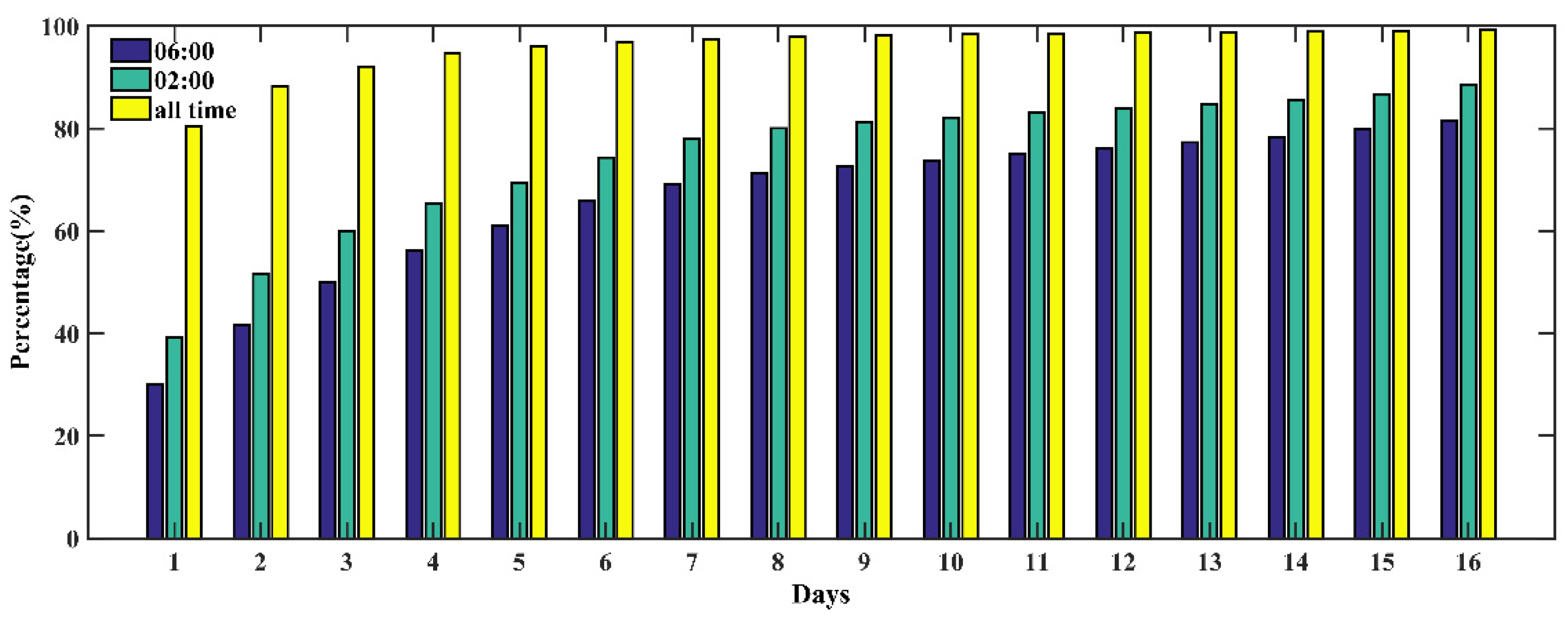
The advantages of compositing clear pixels from the geostationary satellites can be illustrated in Figure 3. Here, AHI cloud products are used for identifying the clear pixels. For one-day composite, the percentage of clear pixel percent increases from 35 to 40% in a single time (10:00 a.m. and 2:00 p.m.) to about 80% in all times. In a 16-day period, the clear percentage is close to 80% for a single time to 100% in all times. This proves that the high-frequency AHI observations greatly reduce the influence of cloud cover on vegetation index retrieval.
2.4. Atmospheric Correction
Atmospheric correction is an important step in the retrieval of vegetation index from AHI. Absorption and scattering of gases and aerosols interfere with the radiation from the Earth to the satellite. In general, absorption attenuating the radiation while scattering redirects the radiation. In previous studies, various techniques are developed to remove the absorption and scattering effects of the atmosphere to obtain the true surface reflectance. Currently, the commonly used atmospheric correction method is based on the 6S radiative transfer model [16].
Assume that the surface reflection is a Lambertian type, the TOA reflectance can be described by:
where and are the cosine values of the solar zenith angle and satellite viewing angle, respectively; is the difference of the sun and satellite azimuthal angle. is the apparent reflectance at the top of the atmosphere after radiation correction and solar zenith angle correction of the signal received by the satellite sensor, is the radiant reflectance of the path composed of atmospheric molecular scattering (Rayleigh Scattering), is the surface reflectance, is the atmospheric transmission rate due to ozone absorption, is the atmospheric water vapor transmission rate, and are the downward radiation transmission rate of atmospheric molecules and the upward radiation transmission rate of atmospheric molecules, respectively.
A comprehensive look-up table (LUT) will be created to perform the atmospheric correction with a high computation efficiency and accuracy. In this study, the inputs of LUT consist of 8 continental absorbing aerosols with optical depths of 0.05, 0.1, 0.2, 0.4, 0.8, 1.2, 1.6, and 2.0, 13 solar zenith angles ranging from 0 to 80° with an interval of 6°, 13 view zenith angles ranging from 0 to 80° with an interval of 6°, and 11 relative azimuth angles from 0 to 180° with an interval of 18°. In addition, the outputs include the transmittance of molecule, ozone, water vapor, upwelling and downwelling radiation, and reflectance of aerosol at TOA. In the algorithm, LUT values are used to obtain the various parameters in Equation (2) with atmospheric state variables, and actual solar and satellite angles. The US standard atmospheric profiles of temperature, water vapor, and ozone are used in radiative transfer calculations. The AOD concentration is obtained from the AHI green band and converted from an optical thickness of 500 nm to an optical thickness of 550 nm by the angstrom exponent formula, Equation (3).
where is the angstrom exponent, is the AOD value of the unknown waveform, is the AOD value of the known waveform. Finally, the corrected surface reflectance can be accurately computed from Equation (2).
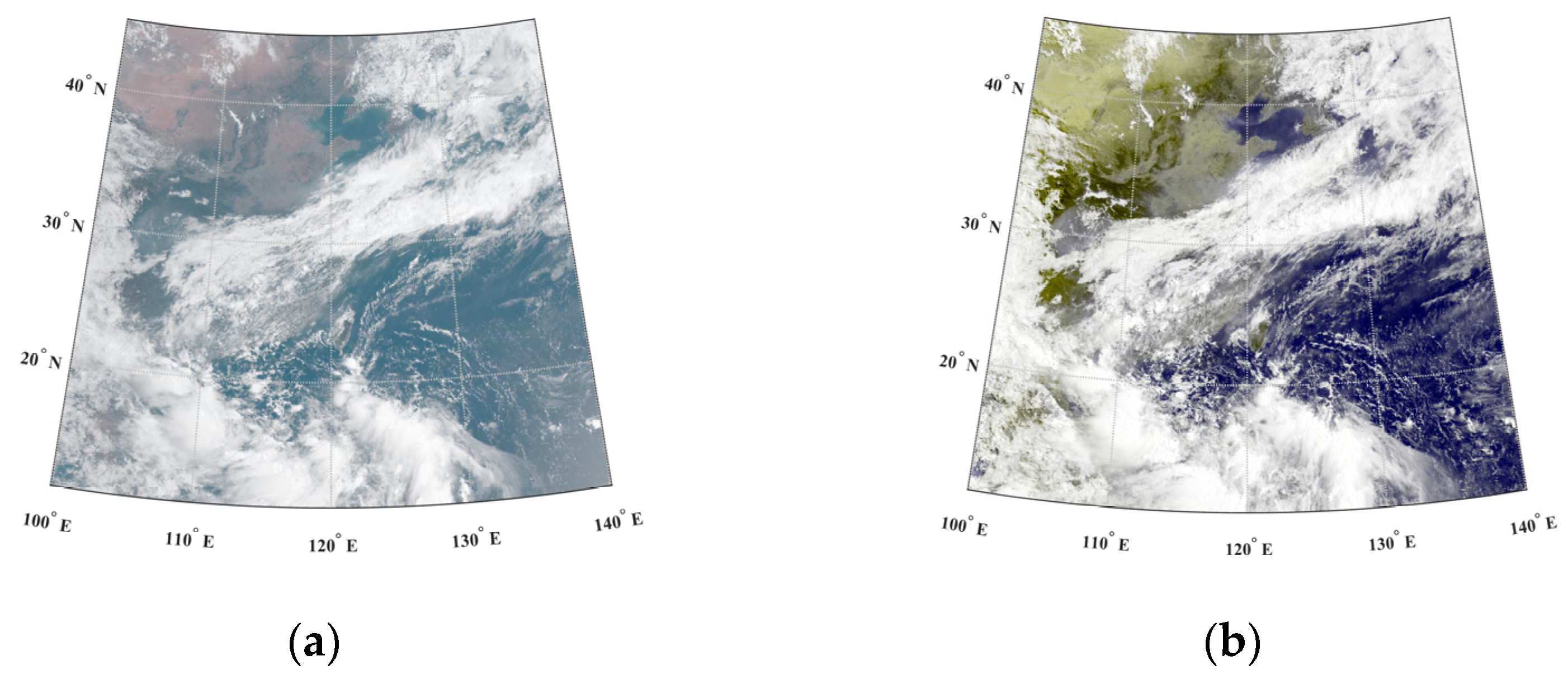
Taking the example of 1 July 2019 with an area of latitude range from 15 N to 45 N, longitude from 100 E to 140 E, Figure 4 compares the true color composite images produced from AHI red, green, and blue band data before and after atmospheric correction. A comparison of the true color composite maps before and after the atmospheric revision shows that the atmospheric correction can remove a layer of milky white fog from the maps, making the landscape clearly identified.
2.5. Angle Correction
The observation angle of a geostationary satellite instrument like AHI at a specific location is typically fixed, but its solar zenith angle changes during the day. Due to the earth’s curvature effect, the solar zenith angle usually changes dramatically with time in low latitudes. In high latitudes, the solar zenith angles are very high. These angle changes are not conducive to the accurate inversion of vegetation index. At the same time, even at the same observation time, the solar zenith angle at different positions are very different, which makes it difficult to compare the retrieved vegetation index. Although the zenith angle of a geostationary satellite is essentially invariant, the values in different regions can vary significantly. Figure 5a,b illustrate the changes of NDVI with solar zenith angle and satellite zenith angle, respectively. Here, the PROSAIL radiative transfer model is obtained by coupling the PROSPECT leaf model with the SAIL canopy structure model. The PROSPECT model [17] is a leaf optical model developed on the basis of the Allen flat plate model. The leaf is assumed to be superimposed by N isotropic layers, with the middle layer divided by N-1 air spacers and the upper layer of the first layer being the leaf epidermis. There exist non-diffuse properties of light, i.e., non-isotropic, while in the interior of the leaf, light is considered isotropic. The PROSPECT model is used to simulate the optical properties of the leaf at 400–2500 nm. In the PROSAIL leaf optical model, a total of 15 parameters including leaf structure, leaf area index (LAI), contents of chlorophyll, brown pigment, water and dry matter, and refractive index are essential for computing the leave optical thickness. In addition, PROSAIL also requires solar zenith and sensor viewing angles, and solar and sensor azimuthal angles in simulation.
From Figure 3, we can see that the NDVI highly varies with both angles, and the NDVI value varies within 20% or more. This effect is more pronounced on the surface where the leaves have high orientations. In order to reduce the uncertain nature of NDVI brought by the sun–target–satellite angle, we use a parameterized BRDF model to correct the angle effects on inversion of vegetation index products.
The BRDF model has three terms representing, respectively, the isotropic, geometric (shading effects) and volumetric (multiple reflections) contributions.
where and are the cosine values of the solar zenith angle and satellite viewing angle, respectively; is the difference of the sun and satellite azimuthal angle. In Equation (4), the first term corresponds to diffuse reflection by material surfaces, of reflectance , which takes into account the geometrical structure of opaque reflectors and shadowing effects. This component is modeled here by vertical opaque protrusions reflecting according to Lambert’s law, placed on a flat horizontal plane. They represent mainly irregularities and roughness of bare soil surfaces, but may also represent structured features of low transmittance canopies. This model has been adopted for its capability to describe simply the shadowing effects. The second term is a component of volumetric scattering, of reflectance , where the medium is modeled as a collection of randomly located facets absorbing and scattering radiation. The facets represent mainly leaves of canopies, characterized by a non-negligible transmittance, but can also model the behavior of dust, fine structures, and porosity of bare soils. A simple radiative transfer model is used to describe this component. One of these kernels, , is derived from volume scattering radiative transfer models [18] and the other, from surface scattering and geometric shadow casting theory [19]. Several studies have identified this RossThick–LiSparse–Reciprocal kernel combination as the model best suited for the operational MODIS BRDF/Albedo algorithm [20,21,22]. The detailed calculation method of each kernel function in the formula will be placed in Appendix A. The BRDF function combined with the coefficients of the MCD43 product can well revise the variation of reflectance with angle. In order to retain the information obtained from the observations, the surface reflectance is corrected through the following expression as
where ) represents the BDRF values corresponding to the solar and satellite zenith angles of zero degree, and azimuthal angle of zero degree.
3. Results
The coefficients in the BRDF model are based on MODIS products in MCD43 and are used for correcting AHI TOA reflectance from the satellite zenith angle and solar zenith angle to the values given in Equation (5). Again, the data from Figure 1 are used for illustration.
We chose the area with a clear sky for almost a whole day on 1 July 2019 to show the effect of angle correction. The study area takes Shandong Province, China, as the theme, and the longitude and latitude range is in latitude 34–39, longitude 114–122. Figure 6a–f shows the red-band reflectance computed from the BRDF model and the atmospheric correction. It can be seen that, as the time changes, the solar zenith angle gradually decreases, the observed reflectance then becomes progressively smaller. This trend is consistent with PROSAIL simulations that the reflectance due to angle changes leads to NDVI change. Also, Figure 6a–c, the BRDF model based on the MODIS coefficients, can simulate the variation of the red-band reflectance very well, both in terms of its magnitude and distribution, and is well comparable with the AHI observations. Next, the reflectance of the AHI red band after atmospheric correction is further corrected using Equation (5) and is shown in Figure 6g–i. It is well demonstrated that the red-band reflectance is less dependent on UTC time.
Figure 7d–f shows the AHI surface reflectance at the near-infrared (NIR) band after atmospheric and angle corrections; as a key channel for the land NDVI, the NIR channel. The change of angle also causes the change of reflectivity. With a decrease of the solar zenith angle from Figure 7a to Figure 7c, the reflectivity becomes smaller. In Figure 7a–f, the comparison shows that the variation pattern of the simulated reflectance from MODIS coefficients with solar zenith angle is generally consistent with the actual observation. The actual observed surface reflectance of AHI at 00:00 UTC and 02:00 UTC is slightly larger than the simulated surface reflectance, which may be due to the limitation of the extrapolation of the BRDF model in the NIR band when the solar zenith angle is larger than a certain threshold (usually around 63.5 degrees). Similarly, using Equation (5), we obtain the results of the reflectance of the AHI in the NIR band after the angular correction. It can be seen that the variation of the reflectance with the solar zenith angle is greatly reduced, compared to the actual observations in Figure 7a–c. Pronounced angular dependent reflectance at 02:00 UTC to 04:00 UTC is corrected to the values at the near-constant level.
After angular and atmospheric corrections, the reflectance of the corresponding band is synthesized according to the time period. It should be mentioned the accuracy of the BRDF model decreases with the increase of both solar and satellite zenith angles [23]. Therefore, in this paper, we use only those pixels when their satellite and solar zenith angles are less than 65 degrees.
Figure 8 shows one-day composite AHI red-band reflectance. For a comparison, the MODIS BRDF products from 16-day composite are normalized to 0 degree and shown in Figure 9.
In general, the reflectance synthesized from AHI single-day agrees with the reflectance of MODIS 16-day composite in terms of both magnitude and spatial patterns. However, more fine structures that identified AHI 1-day composite data are missing in MODIS products.
With the synthetic reflectance, we calculate the NDVI according to Equation (1), as shown in Figure 10. The spatial distributions of NDVI at different times are compared before and after the angular corrections. The NDVI increases as the solar zenith angle decreases. This is consistent with the results of the PROSAIL simulations in the previous section. After angle correction, the NDVI pattern becomes less affected by angle. From the above comparison results, it can be seen that the angular correction can bring good benefits in the retrieval of land surface vegetation index using AHI from high-frequency observations.
Figure 11a shows NDVI composited from AHI single-day reflectance. Because AHI can observe the same area many times in a day, the influence of clouds on the products is greatly reduced. About 80% of clear sky pixels can be used for NDVI synthesis from one day of observations. Compared with the single time observations shown as Figure 11b, the vegetation monitoring is limited to a smaller area under a clear sky condition. The quantitative comparison is given by the scatter plot in Figure 11c,d; the correlation between the two products can reach 0.9206, while the RMSE is only 0.1149. Thus, it can be demonstrated that the vegetation indices inverted from AHI observations are well comparable with those calculated by MODIS BRDF fitting.
4. Discussion and Conclusions
Monitoring land vegetation conditions are made possible through polar-orbiting satellites through retrievals of surface vegetation index. However, few studies have been attempted from using geostationary satellites for surface vegetation studies. As we are paying great attention to ecosystem monitoring in both space and time, the demand for more frequent monitoring vegetation is increasing. For example, in cases of forest fires, floods, cyanobacteria outbreaks in inland lakes, etc., the use of high-frequency geostationary satellite observations can greatly reduce cloud effects and get a higher temporal resolution of the vegetation products. As the spatial resolution of geostationary satellites imager has greatly improved in the past decades and more geostationary satellites are launched in various countries and are carrying onboard advanced instruments (e.g., AHI and AGRI), more high quality of land surface products can be derived. This study proposes a new method for deriving NDVI from the geostationary satellite imager (AHI). AHI reflectance at the top of the atmosphere is corrected to the surface reflectance through a radiative transfer model. The effects of the AHI satellite zenith angle and solar zenith angles on the NDVI are corrected. Sine AHI observations can identify more clear pixels during a day, and more surface NDVI pixels can be derived. It is demonstrated that at least 80% of land can be monitored from a single day of AHI observations, whereas less than 30% can be viewed from a single polar-orbiting satellite. The advantage of using the geostationary data is clearly illustrated from this research. At the same time NDVI derived from AHI observations are well comparable with those calculated by MODIS 16 days.
Author Contributions
Conceptualization, F.W.; methodology, S.L. and F.W.; validation, S.L. and X.H.; writing—original draft preparation, S.L.; writing—review and editing, F.W. All authors have read and agreed to the published version of the manuscript.
Funding
This research was funded by the National Key Research and Development Program of China (2021YFB3900400) and the National Natural Science Foundation of China (U2142212).
Data Availability Statement
The AHI data can be download from the website of JAXA (JAXA Himawari Monitor (P-Tree System). Available online: https://www.eorc.jaxa.jp/ptree/). The MCD43 dataset can be download from the website of LAADS DAAC (Find Data—LAADS DAAC (nasa.gov). Available online: https://ladsweb.modaps.eosdis.nasa.gov/missions-and-measurements/products/MCD43A3).
Acknowledgments
We thank Hao Hu, Yang Han, Yining Shi and Chuanwen Wei for Provide suggestion in this work. We also sincerely thank the reviewers and editors for their insightful comments.
Conflicts of Interest
The authors declare no conflict of interest.
Appendix A
On the detailed calculation method of each kernel function in Formula (4).
where
References
- Analysis of the Vegetation Cover Change and the Relationship between NDVI and Environmental Factors by Using NOAA Time Series Data. J. Remote Sens. 1998, 266, 153.
- Huete, A.; Didan, K.; Miura, T.; Rodriguez, E.P.; Gao, X.; Ferreira, L.G. Overview of the radiometric and biophysical performance of the MODIS vegetation indices. Remote Sens. Environ. 2002, 83, 195–213. [Google Scholar] [CrossRef]
- Brown, M.E.; Pinzón, J.E.; Didan, K.; Morisette, J.T.; Tucker, C.J. Evaluation of the consistency of long-term NDVI time series derived from AVHRR, SPOT-vegetation, SeaWiFS, MODIS, and Landsat ETM+ sensors. IEEE Trans. Geosci. Remote Sens. 2006, 44, 1787–1793. [Google Scholar] [CrossRef]
- Deering, D.W. Rangeland Reflectance Characteristics Measured by Aircraft and Spacecraft Sensors. Ph.D. Dissertation, Texas A&M Universtiy, College Station, TX, USA, 1978. [Google Scholar]
- Tong, S.; Zhang, J.; Bao, Y. Spatial and temporal variations of vegetation cover and the relationships with climate factors in Inner Mongolia based on GIMMS NDVI3g data. J. Arid. Land 2017, 9, 394–407. [Google Scholar] [CrossRef] [Green Version]
- Fensholt, R.; Sandholt, I.; Rasmussen, M.S. Evaluation of MODIS LAI, fAPAR and the relation between fAPAR and NDVI in a semi-arid environment using in situ measurements. Remote Sens. Environ. 2004, 91, 490–507. [Google Scholar] [CrossRef]
- Vargas, M.; Miura, T.; Shabanov, N.; Kato, A. An initial assessment of Suomi NPP VIIRS vegetation index EDR. J. Geophys. Res. Atmos. 2013, 118, 12301–12316. [Google Scholar] [CrossRef] [Green Version]
- Skakun, S.; Justice, C.O.; Vermote, E.; Roger, J.C. Transitioning from MODIS to VIIRS: An analysis of inter-consistency of NDVI data sets for agricultural monitoring. Int. J. Remote Sens. 2018, 39, 971–992. [Google Scholar] [CrossRef]
- Miura, T.; Muratsuchi, J.; Vargas, M. Assessment of cross-sensor vegetation index compatibility between VIIRS and MODIS using near-coincident observations. J. Appl. Remote Sens. 2018, 12, 045004. [Google Scholar] [CrossRef]
- Lunetta, R.S.; Knight, J.F.; Ediriwickrema, J. Land-cover characterization and change detection using multitemporal MODIS NDVI data. Remote Sens. Environ. 2009, 105, 142–154. [Google Scholar] [CrossRef]
- Bessho, K.; Date, K.; Hayashi, M.; Ikeda, A.; Imai, T.; Inoue, H.; Kumagai, Y.; Miyakawa, T.; Murata, H.; Ohno, T.; et al. An Introduction to Himawari-8/9—Japan’s New-Generation Geostationary Meteorological Satellites. J. Meteorol. Soc. Jpn. Ser. II 2016, 94, 151–183. [Google Scholar] [CrossRef] [Green Version]
- Liu, H.; Zhou, Q.; Zhang, S.; Deng, X. Estimation of Summer Air Temperature over China Using Himawari-8 AHI and Numerical Weather Prediction Data. Adv. Meteorol. 2019, 2019, 2385310. [Google Scholar] [CrossRef] [Green Version]
- Wang, J.; Jiao, Z.; Feng, G.; Xie, L.; Yan, G.; Xiang, Y.; Liang, S.; Li, S. Validation of MODIS Albedo Product by Using Field Measurements and Airborne Multi-Angular Remote Sensing Observations. In Proceedings of the 2003 IEEE International Geoscience and Remote Sensing Symposium. Proceedings (IEEE Cat. No.03CH37477), Toulouse, France, 21–25 July 2003. [Google Scholar]
- Wang, Z.; Schaaf, C.B.; Sun, Q.; Shuai, Y.; Román, M.O. Capturing rapid land surface dynamics with Collection V006 MODIS BRDF/NBAR/Albedo (MCD43) products. Remote Sens. Environ. 2018, 207, 50–64. [Google Scholar] [CrossRef]
- Nightingale, J.M.; Morisette, J.T.; Wolfe, R.E.; Tan, B.; Gao, F.; Ederer, G.; Collatz, G.J.; Turner, D.P. Temporally smoothed and gap-filled MODIS land products for carbon modelling: Application of the fPAR product. Int. J. Remote Sens. 2009, 30, 1083–1090. [Google Scholar] [CrossRef]
- Vermote, E.F.; Tanré, D.; Deuze, J.L.; Herman, M.; Morcette, J.J. Second simulation of the satellite signal in the solar spectrum, 6S: An overview. IEEE Trans. Geosci. Remote Sens. 1997, 35, 675–686. [Google Scholar] [CrossRef] [Green Version]
- Jacquemoud, S.; Baret, F.; Andrieu, B.; Danson, F.M.; Jaggard, K. Extraction of vegetation biophysical parameters by inversion of the PROSPECT + SAIL models on sugar beet canopy reflectance data. Appl. TM AVIRIS Sens. Remote Sens. Environ. 1995, 52, 163–172. [Google Scholar] [CrossRef]
- Jacquemoud, S.; Baret, F. PROSPECT: A model of leaf optical properties spectra. Remote Sens. Environ. 1990, 34, 75–91. [Google Scholar] [CrossRef]
- Roujean, J.L.; Leroy, M.; Deschanps, P.Y. A bidirectional reflectance model of the Earth’s surface for the correction of remote sensing data. J. Geophys. Res. Atmos. 1992, 972, 20455–20468. [Google Scholar] [CrossRef]
- Li, X.; Strahler, A.H. Geometric-optical bidirectional reflectance modeling of the discrete crown vegetation canopy: Effect of crown shape and mutual shadowing. IEEE Trans. Geosci. Remote Sens. 1992, 30, 276–292. [Google Scholar] [CrossRef]
- Lucht, W.; Schaaf, C.; Strahler, A.H.; d’Entremont, R. Remote Sensing of Albedo Using the BRDF in Relation to Land Surface Properties. In Observing Land from Space: Science, Customers and Technology; Verstraete, M.M., Menenti, M., Peltoniemi, J., Eds.; Springer: Dordrecht, The Netherlands, 2000; pp. 175–186. [Google Scholar]
- Privette, J.L.; Eck, T.F.; Deering, D.W. Estimating spectral albedo and nadir reflectance through inversion of simple BRDF models with AVHRR/MODIS-like data. J. Geophys. Res. Atmos. 1997, 102, 29529–29542. [Google Scholar] [CrossRef]
- Wanner, W.; Strahler, A.H.; Hu, B.; Lewis, P.; Muller, J.-P.; Li, X.; Barker Schaaf, C.L.; Barnsley, M.J. Global retrieval of bidirectional reflectance and albedo over land from EOS MODIS and MISR data: Theory and algorithm. In Passive Remote Sensing of Tropospheric Aerosol and Atmospheric Corrections From the New Generation of Satellite Sensors; American Geophysical Union: Washington, DC, USA, 1997. [Google Scholar]
Figure 1.
Spectrum response function for red and near-infrared bands of the AHI onboard Himawari-8 satellite and the MODIS on board AQUA satellite.
Figure 1.
Spectrum response function for red and near-infrared bands of the AHI onboard Himawari-8 satellite and the MODIS on board AQUA satellite.

Figure 2.
Synthesis of AHI observation of clear sky areas in latitude 0–60, longitude 80–160, and the white points are the pixel with clouds during the 16-day synthetic period of observation: (left) synthesis with 10:00 a.m. local observation time only; (mid) synthesis with 2:00 p.m. local observation time only; (right) synthesis of all observation moments throughout the day.

Figure 3.
AHI observations over 16 days of compositing period. The color bars represent the percent of AHI clear pixels in our study domain, as defined in Figure 2.
Figure 3.
AHI observations over 16 days of compositing period. The color bars represent the percent of AHI clear pixels in our study domain, as defined in Figure 2.

Figure 4.
AHI true color composite imagery (a) before atmospheric correction and (b) after atmospheric correction.
Figure 4.
AHI true color composite imagery (a) before atmospheric correction and (b) after atmospheric correction.

Figure 5.
Variation of NDVI with angle simulated by PROSAIL (the main setting parameters are as follows: chlorophyll content = 40 (ug.cm−2); carotenoid content = 8 (ug.cm−2); brown pigment content = 0.0 (arbitrary units); equivalent water thickness = 0.01 (cm); dry matter content = 0.009 (g.cm−2); leaf structure parameter = 2.5; leaf area index = 0.5 (m2/m2); hot pot = 0.01). (a) Variation of NDVI with solar zenith angle and (b) Variation of NDVI with satellite zenith angle.

Figure 6.
(a–c) are the AHI red-band reflectance at 00:00 UTC, 02:00 UTC and 04:00 UTC on 1 July 2019 computed from mcd43 coefficient respectively. (d–f) correspond to the reflectance after atmospheric correction. (g–i) are the reflectance after both atmospheric and angle corrections.
Figure 6.
(a–c) are the AHI red-band reflectance at 00:00 UTC, 02:00 UTC and 04:00 UTC on 1 July 2019 computed from mcd43 coefficient respectively. (d–f) correspond to the reflectance after atmospheric correction. (g–i) are the reflectance after both atmospheric and angle corrections.

Figure 7.
(a–c) are the AHI near-infrared band reflectance at 00:00 UTC, 02:00 UTC and 04:00 UTC on 1 July 2019 computed from MCD43 coefficient, respectively. (d–f) correspond to the reflectance after atmospheric correction. (g–i) are the reflectance after both atmospheric and angle corrections.
Figure 7.
(a–c) are the AHI near-infrared band reflectance at 00:00 UTC, 02:00 UTC and 04:00 UTC on 1 July 2019 computed from MCD43 coefficient, respectively. (d–f) correspond to the reflectance after atmospheric correction. (g–i) are the reflectance after both atmospheric and angle corrections.

Figure 8.
AHI composited reflectance at red band on 1 July 2019. (a) red band and (b) NIR.

Figure 9.
MODIS 16-day composite reflectance normalized to 0 degrees on 1 July 2019; (a) red band and (b) near-infrared band.
Figure 9.
MODIS 16-day composite reflectance normalized to 0 degrees on 1 July 2019; (a) red band and (b) near-infrared band.

Figure 10.
NDVI derived from AHI (a) 00:00 UTC, (b) 02:00UTC and (c) 04:00 UTC before angle correction. (d–f) are corresponding NDVI after AHI angle correction.
Figure 10.
NDVI derived from AHI (a) 00:00 UTC, (b) 02:00UTC and (c) 04:00 UTC before angle correction. (d–f) are corresponding NDVI after AHI angle correction.

Figure 11.
(a) Composite NDVI products from (a) one day of AHI data, (b) a single time (00:00 UTC on 1 July 2019) NDVI, (c) composite NDVI products from 16 days MODIS and (d) a comparison of the AHI one day and MODIS 16 days.
Figure 11.
(a) Composite NDVI products from (a) one day of AHI data, (b) a single time (00:00 UTC on 1 July 2019) NDVI, (c) composite NDVI products from 16 days MODIS and (d) a comparison of the AHI one day and MODIS 16 days.


Table 1.
Advanced Himawari Imager characteristics and their major applications.
| Channel | Center Wavelength (μm) | Channel Name | Spatial Resolution (m) | Major Applications |
|---|---|---|---|---|
| 1 | 0.47 | Blue | 1000 | Vegetation, Aerosols, True color image |
| 2 | 0.51 | Green | 1000 | |
| 3 | 0.64 | Red | 500 | Cloud, True color image |
| 4 | 0.86 | NIR | 1000 | Vegetation, Aerosols |
| 5 | 1.6 | IR | 2000 | Cloud type |
| 6 | 2.3 | Cloud particle effective radius | ||
| 7 | 3.9 | Cloud, Fog, Fire | ||
| 8 | 6.2 | Water vapor | ||
| 9 | 6.9 | |||
| 10 | 7.3 | |||
| 11 | 8.6 | Cloud type, SO2 | ||
| 12 | 9.6 | O3 | ||
| 13 | 10.4 | Cloud, Cloud top | ||
| 14 | 11.2 | Cloud, SST | ||
| 15 | 12.4 | |||
| 16 | 13.3 | Cloud, CHT |
Publisher’s Note: MDPI stays neutral with regard to jurisdictional claims in published maps and institutional affiliations. |
© 2022 by the authors. Licensee MDPI, Basel, Switzerland. This article is an open access article distributed under the terms and conditions of the Creative Commons Attribution (CC BY) license (https://creativecommons.org/licenses/by/4.0/).
Share and Cite
MDPI and ACS Style
Li, S.; Han, X.; Weng, F. Monitoring Land Vegetation from Geostationary Satellite Advanced Himawari Imager (AHI). Remote Sens. 2022, 14, 3817. https://doi.org/10.3390/rs14153817
AMA Style
Li S, Han X, Weng F. Monitoring Land Vegetation from Geostationary Satellite Advanced Himawari Imager (AHI). Remote Sensing. 2022; 14(15):3817. https://doi.org/10.3390/rs14153817
Chicago/Turabian StyleLi, Shengqi, Xiuzhen Han, and Fuzhong Weng. 2022. "Monitoring Land Vegetation from Geostationary Satellite Advanced Himawari Imager (AHI)" Remote Sensing 14, no. 15: 3817. https://doi.org/10.3390/rs14153817
Note that from the first issue of 2016, this journal uses article numbers instead of page numbers. See further details here.